Virtual 3D Multi-Angle Modeling and Analysis of Nighttime Lighting in Complex Urban Scenes

Abstract

Urban nighttime lighting extends human activity hours and enhances safety but also wastes energy and causes light pollution. Influenced by building obstructions and surface reflections, light emissions exhibit significant anisotropy. Remote sensing can be used to observe nighttime lighting from high altitudes, but ground lighting anisotropy introduces angle-related errors. This study constructed a 3D urban nighttime lighting model using virtual simulations and conducted multi-angle observations to investigate anisotropy and its influencing factors. The results show that the illuminance distribution in urban functional areas is typically uneven, with ground-level illuminance varying linearly or exponentially with zenith angle and quadratically with azimuth angle. Some areas exhibit uniform illuminance without significant anisotropy. Nighttime light anisotropy is closely linked to urban geometry and light distribution, with building height, layout, and light source arrangement significantly influencing the anisotropic characteristics. The findings enhance our understanding of nighttime light anisotropy, provide a basis for developing angular effect models of complex scenarios, and quantify the upward light emission angles and intensities. These insights can be used to support corrections for multi-angle spaceborne nighttime lighting observations, contributing to more accurate data for urban planning and light pollution mitigation.

1. Introduction

With the rapid acceleration of global urbanization, nighttime activities are playing an increasingly important role in urban life. Urban nighttime lighting not only extends human activity hours but also provides residents with a relatively safe environment, fostering economic, social, and cultural activities. However, the excessive and disordered use of urban lighting has also led to problems such as energy waste and environmental pollution. Among these, nighttime light emissions into the sky are a major source of skyglow pollution [1]. This not only disrupts the natural darkness of the night sky but also increases the risk of health issues in humans [2]. Moreover, due to the anisotropy of nighttime lighting, its impacts on flora and fauna are particularly pronounced. For instance, upward-scattered light attracts insects and birds, interfering with their migration routes, while intense lateral lighting disrupts the hunting behaviors of nocturnal animals, affecting their survival and reproduction [3,4,5]. In terms of light pollution management, although many cities have adopted energy-efficient lighting such as LED lights to reduce energy consumption, severe light pollution persists due to the lack of control over the light direction [6]. Balancing urban lighting functionality while avoiding energy waste and reducing skyglow pollution has become a key concern for urban managers and researchers around the world. Therefore, it is crucial to clarify the sources and influencing factors of nighttime light emissions. However, due to the complex sources of urban nighttime light emissions into the sky, the diverse geometric structures of urban surfaces, and the multiple reflections of nighttime light within urban built environments, quantitatively analyzing nighttime light emissions remains a significant challenge.

Early studies on the quantitative analysis of nighttime light emissions primarily focused on their impact on astronomical observations. These studies generally employed ground-based observations and simulation models to analyze light emissions above urban areas [7,8,9]. Kocifaj proposed a scalable theoretical model for light pollution from ground-based sources. This model, applicable to both cloudy and clear night skies, simulates the angular behavior of spectral and overall sky radiance and luminance while considering atmospheric effects on transmitted radiation as well as aerosol and molecular optical properties [10]. However, such ground-based observation models primarily focus on the effects of skyglow and do not delve into the internal dynamics of urban environments. Consequently, they fall short of accurately identifying the sources of nighttime light emissions contributing to light pollution.

As a result, technologies for monitoring nighttime light emissions from urban areas have emerged. Scientists have utilized remote sensing satellite technologies to monitor urban nighttime lighting, explore the spatial distribution of human activities, and assess their ecological and environmental impacts. Currently, the main nighttime light remote sensing products include the Defense Meteorological Satellite Program/Operational Linescan System (DMSP/OLS), the Visible Infrared Imaging Radiometer Suite (VIIRS) onboard the Suomi National Polar-orbiting Partnership (NPP) satellite, Jilin-1, Luojia-1, and SDGsat. These products provide researchers with abundant nighttime light data, enabling them to understand the spatial distribution and dynamics of urban nighttime light emissions and apply the data across various research domains. The key applications include the assessment of light pollution [11,12]; modeling and spatialization of socioeconomic, demographic, and environmental variables such as CO₂ emissions [13,14,15,16,17]; analysis of changes in human activities during disasters, armed conflicts, and holidays [18,19]; and urban mapping [20,21,22,23]. Other applications include studies on power supply [24] and marine fisheries [25]. However, the nighttime light radiation observed by spaceborne remote sensing instruments exhibits significant differences across various viewing angles, demonstrating pronounced anisotropy. This is because near-ground lighting not only emits in the downward direction, but also scatters upward, laterally, and in surrounding directions. Additionally, building façades contribute substantially to nighttime light emissions. Such anisotropy not only exacerbates the diffusion of light pollution but also leads to greater energy wastage [26].

To quantitatively study the anisotropy of spaceborne remote sensing, some researchers have attempted to use multi-angle observations over repeated cycles to reveal the anisotropic characteristics of nighttime light emissions. These studies have found that the influencing factors are primarily related to the zenith angle, with noticeable cold and hot spot effects in the nighttime brightness of urban built-up areas [27,28]. Other studies have shown that the anisotropy of urban nighttime light emissions is closely related to urban functional zones. The height of buildings determine the obstructed and visible portions of artificial light, and the anisotropy of nighttime light emissions is jointly influenced by the light sources and landscape morphology [29]. Additionally, research indicates that nighttime light radiation in urban areas may exhibit distinct angular emission profiles depending on the urban landscape, such as high-rise buildings, trees, and vertical light sources [30,31,32,33]. However, these analyses, based on statistical data from multiple spaceborne revisit cycles, do not account for variations in weather and atmospheric aerosols. This makes it challenging to reproduce nighttime light radiation values for the same time period under identical observation conditions and arbitrary viewing angles. To better understand the spatial distribution of urban nighttime lighting and the full scope of light pollution, researchers have recently begun using multi-angle observation techniques. Multi-angle remote sensing technology, which captures ground-reflected light from different angles, can more accurately capture the anisotropic characteristics of urban lighting, particularly the intensity of light radiation in various directions [10,34]. Drone platforms, with their flexibility, allow researchers to mount multi-angle sensors on drones, enabling detailed analyses of the radiative characteristics of urban lighting in all directions. This provides a new approach for comprehensively understanding and mitigating light pollution [35,36]. However, the widespread application of drones is currently restricted in many urban areas due to safety concerns.

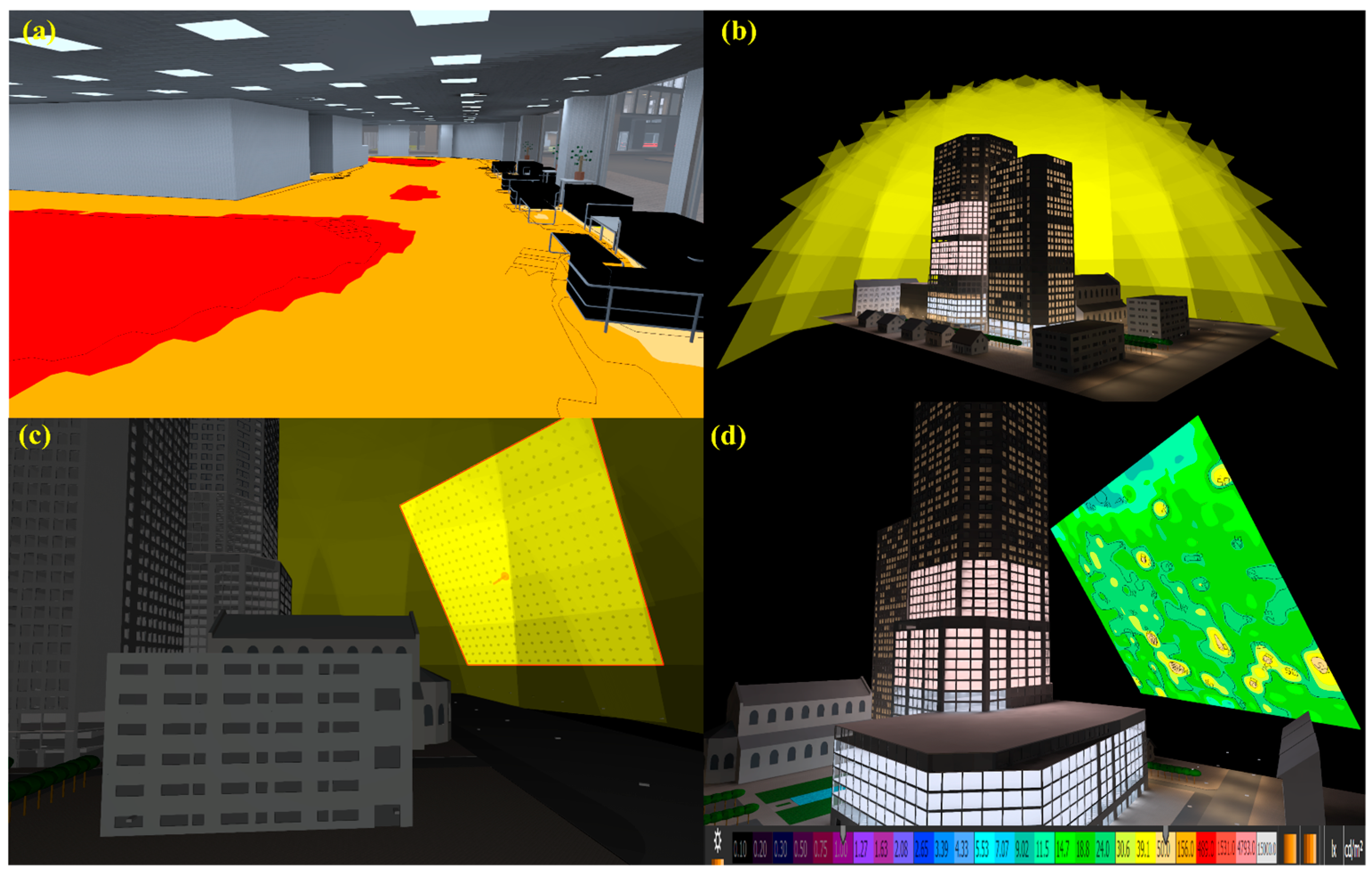
In this context, three-dimensional nighttime light scene modeling based on virtual simulations has emerged as an effective alternative. This technique enables the construction of various complex urban lighting scenarios and facilitates simulation observations from arbitrary angles, effectively addressing the limitations of ground-based observations and providing a viable approach for the multi-angle quantitative analysis of urban nighttime light emissions. For instance, Kim employed computer simulations to analyze upward light produced by large-scale lighting in sports facilities and proposed a method for defining a virtual horizontal plane above stadiums [37]. Jin et al. conducted a study in the Beijing “The Place” mixed-use district and introduced a low-cost, easy-to-implement, and rapid data-analysis method for assessing light pollution [38]. Similarly, Jimmy C.K. Tong and his research team utilized DIALux evo 9 software to develop urban lighting models, examining light pollution on urban streets and light intrusion into building façades in Hong Kong [39,40,41,42]. These studies have provided valuable data and methodological support for quantifying and assessing urban light pollution, contributing to a more intuitive understanding of nighttime light anisotropy. However, the mechanisms underlying the anisotropy of nighttime light emissions and observation angles in complex urban scenarios remain unclear. Additionally, the ways in which urban ground geometries and nighttime light source distributions influence nighttime light emission patterns have yet to be fully understood. Therefore, it is imperative to employ virtual 3D scene modeling to establish multi-angle models of nighttime lighting in complex urban environments, enabling the quantitative analysis of nighttime light emissions and their influencing factors.

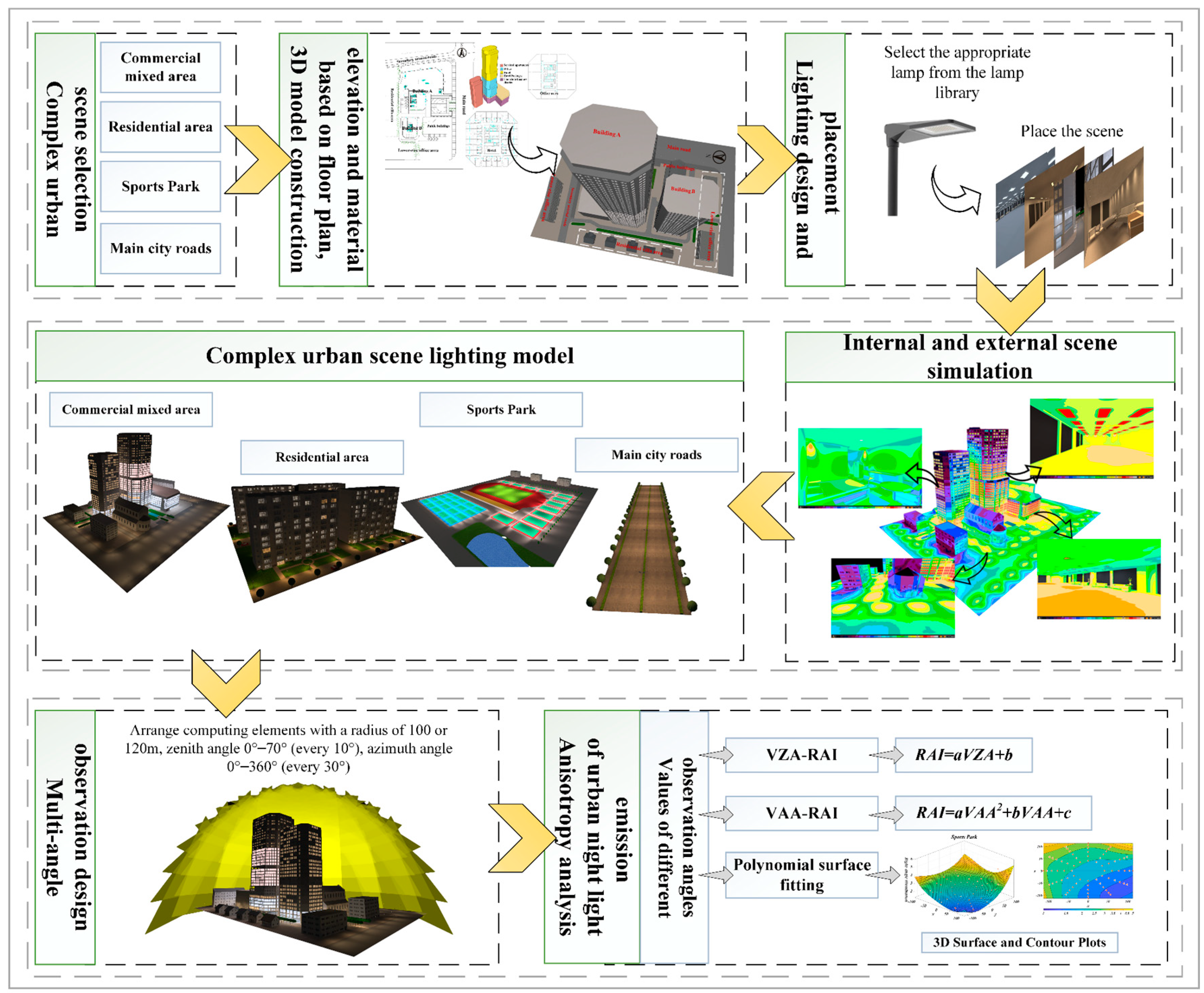
In summary, although the existing research has made preliminary explorations into the anisotropy of nighttime lighting, there are still several limitations: (1) existing methods largely rely on statistical analyses of spaceborne remote sensing data, lacking detailed modeling of the ground-level light propagation process; (2) most studies focused primarily on the impact of the zenith angle on nighttime light distribution, while overlooking the role of the azimuth angle; and (3) there is a lack of comprehensive analyses of urban geometric forms and light distributions, making it difficult to fully reveal the spatial distribution characteristics of nighttime lighting. In this study, we employed virtual 3D scene modeling to construct nighttime lighting scenarios for different urban functional zones. By using various zenith and azimuth angles for the observations, we simulated nighttime light emissions to quantitatively investigate the anisotropy of urban nighttime light emissions. This approach aims to explore the influencing factors of nighttime light emissions in complex urban scenarios.

2. Materials and Methods

As shown in Figure 1, the main steps and tasks in this study were as follows: First, we constructed the urban scene using a layout map and virtual simulation model, and then inserted the necessary light fixtures into each space to simulate the nighttime lighting scenario. Next, computational elements were inserted according to the plan to obtain calculation results for observations from different spatial angles. Finally, the anisotropy of nighttime light emissions in urban functional zones was analyzed. Since this study primarily focused on the anisotropic characteristics and spatial distribution patterns of nocturnal lighting in complex urban environments, the influence of external environmental factors such as weather and aerosols were not considered in the experiments. Instead, modeling and simulation were conducted based on an idealized virtual three-dimensional scene, thereby providing a clearer insight into the spatial distribution characteristics of nocturnal lighting.

2.1. Construction of Nighttime Lighting Model for Complex Urban Scenes

2.1.1. Selection of Complex Urban Scenes and Construction of Three-Dimensional Models

To comprehensively analyze the distribution patterns and anisotropic characteristics of urban nighttime lighting, we selected four complex urban scenarios based on urban functional classifications: commercial mixed areas, residential areas, sports parks, and main city roads. Virtual nighttime lighting scene models were established for each of these scenarios. These selected scenes represent common urban functional zones, each with distinct lighting requirements and layout differences. These scenarios encompass typical lighting usage and characteristics in urban environments, allowing for an effective analysis of the anisotropy of urban nighttime lighting.

The modeling work for the virtual scenes was performed as follows: First, the layout plans for the different functional study areas were drawn (Figure 2a–d). Then, 3D models of the functional scenes were created, such as the 3D model of the commercial mixed-use area shown in Figure 2e. The modeling software used in this study was DIALux evo 12.1. It is a professional lighting design software widely used for simulating and calculating parameters such as light distribution, illuminance, and brightness in lighting scenarios. Due to the complexity of the actual environment, it was difficult to input all parameters of the environment into the software. Therefore, the virtual scenes created in this study were designed to closely approximate the real-world scenarios. The reflection coefficients for building surfaces and the ground were taken from those provided by the software. The reflectance values for the building and road surfaces in the model were fixed, as shown in

Table 1. Reflection coefficients of various materials.

Feature	Reflectivity	Reflective Coating	Effect
Building facade	34%	0%
Window glass	10%	90%
Indoor floor	70%	7%
Indoor wall	50%	0%
Ceiling	56%	0%
Street surface	28%	0%
Building land ground	45%	0%
Green plants	11%	0%
Grassland	15%	0%
Water surface	20%	9%

.

2.1.2. Complex Scene Lighting Arrangement

Due to the different functional classifications of buildings, the selected lighting fixtures varied. In this study, nine types of lighting fixtures, including streetlights, were used; their parameters are shown in

Table 2. Parameters of various lamps.

Lighting Fixtures	Manufacturer	Product Name	P	Φ	Light Efficiency	Light Curve
	Leipziger Leuchten GmbH (Leipzig, Germany)	ALFONS II DA LED (Optik 128)	69.0 W	8945 lm	129.6 lm/W
	Midea (Foshan, China)	MPB36T6060-W 36W 5700K	34.9 W	2688 lm	77.0 lm/W
	NVC (Huizhou, China)	NLED483M 32W (600 × 600 mm) 5700K	32.0 W	2720 lm	85.0 lm/W
	NVC (Huizhou, China)	NLED1193D 3.5W 24°3000K	3.5 W	240 lm	68.6 lm/W
	NVC (Huizhou, China)	NLED1185 5W 38°3000K	5.0 W	230 lm	46.0 lm/W
	NVC (Huizhou, China)	NLED9248A 20W 3000K	21.2 W	1800 lm	84.9 lm/W
	NVC (Huizhou, China)	NLED4504 40W (298 × 1198) 3000K	40.0 W	2800 lm	70.0 lm/W
	NVC (Huizhou, China)	NLED4545 56W W60 4000K	56.0 W	3000 lm	53.6 lm/W
	NVC (Huizhou, China)	NLED4211J-AL 16W 300 × 300 3000K	16.3 W	1100 lm	67.5 lm/W

. For each type of light source, lighting products from the DIALux evo 12.1 fixture library were chosen to simulate the lighting in the model. The luminous flux parameters for each light cluster are adjustable and were set to default values before the first simulation. Each lighting product also has a fixed “luminous output ratio”. The actual luminous flux output, referred to as “fixture luminous flux” in this study, was calculated using the following formula: luminous flux × luminous output ratio [43]. The virtual nighttime lighting scenes in this study were based on real nighttime scenarios, aiming to closely match actual conditions. Some of the lighting distributions in the rooms and spaces are shown in Figure 3.

The purpose of the modeling work was to establish the best model that closely matches the actual lighting conditions. To determine the optimal model, we referred to the “Building Lighting Design Standards” GB/T 50034-2024 [44] issued by the Ministry of Housing and Urban–Rural Development of China, as shown in

Table 3. Standard lighting values for various rooms or places.

Building Category	Room or Place	Reference Plane and Its Height	Illuminance Standard Value (lx)
Commercial buildings	General store sales hall	Horizontal plane, 0.75 m	300
	General indoor shopping street	Surface	200
	High-end store sales hall	Horizontal plane, 0.75 m	500
	General supermarket sales hall	Horizontal plane, 0.75 m	300
	High-end supermarket business hall	Horizontal plane, 0.75 m	500
Hotel building	General activity area of guest room	Horizontal plane, 0.75 m	75
	Chinese restaurant	Horizontal plane, 0.75 m	200
	Western restaurant	Horizontal plane, 0.75 m	150
	Cafe, bar	Horizontal plane, 0.75 m	75
	Hotel lobby	Surface	200
	Swimming pool	Water surface	200
	Treatment room	Horizontal plane, 0.75 m	300
Office building	General office	Horizontal plane, 0.75 m	300
	Meeting room	Horizontal plane, 0.75 m	300
	High-end office	Horizontal plane, 0.75 m	500
Residential buildings	Living room	Horizontal plane, 0.75 m	100
	Bedroom	Horizontal plane, 0.75 m	75
	Dining room	Horizontal plane, 0.75 m	150
Traffic building	Residential road	Surface	15
	Main city roads	Surface	20
Sports building	Basketball court	Surface	300
	Gym	Horizontal plane, 0.75 m	200
	Badminton court	Surface	300
	Football field	Surface	200

. In the various rooms or spaces, work planes were established (Figure 4a), and the lighting fixture parameters were adjusted so that the rooms or spaces involved in the virtual nighttime lighting scene meet the lighting standards and have illuminance levels higher than the standard values.

2.2. Multi-Angle Observation of Complex Scenes

2.2.1. Design of Spatial Observation Angle for Complex Scenes

After establishing the urban complex scene simulation model, the next step was to calculate the multi-angle observation values of the scene. The simulation software’s computational functionality allows for the calculation of key lighting parameters, including illuminance, uniformity, and glare index, based on the input data. The positions of the calculation planes are shown in Figure 5. A reference point in the scene was selected as the center, and a hemisphere with a radius of 120 m was constructed for the commercial mixed-use area, while the other three scenarios were modeled with a hemisphere with a radius of 100 m. Multiple calculation planes were set in these hemispheres. Specifically, in the vertical direction, seven circular planes were selected at zenith angles of 10°, 20°, 30°, 40°, 50°, 60°, and 70°. Starting from the true north direction (azimuth angle of 0°), a calculation plane was set every 30° in the clockwise direction, resulting in 12 calculation planes for each zenith angle. Additionally, a calculation plane was set at the zenith angle of 0° to compute the horizontal illuminance (Figure 4b). Each calculation plane was 100 m × 100 m in size, with 400 evenly distributed calculation points on each plane. The average value of these calculation points was taken as the final result for that plane. This arrangement of calculation planes simulates the spiral flight path of a drone and, considering the altitude restrictions for drones flying over urban areas, the radius was set to 100 m or 120 m.

The calculation parameter selected for this study (Figure 4c,d) was the right-angle illumination (RAI), measured in lux (lx), which is the amount of luminous flux received per unit area perpendicular to the direction of the calculation plane (1 lx = 1 lm/m²). The illuminance unit used in this study is related to radiometric quantities in sky observations, such as radiance and irradiance, but belongs to a different optical measurement system. Lumen and lux are photometric units, whereas radiometric units correspond to radiative quantities. These two measurement systems can be converted into one another, but it is essential to consider how the human eye perceives light at different wavelengths, which is accounted for by the spectral sensitivity function or luminous efficiency function of light. The conversion formula is as follows:

$${\Phi }_v=km{\int }_0^{\mathrm{\infty }}E\left(\lambda \right)V\left(\lambda \right)d\lambda$$

(1)

where ${\Phi }_v$ is the luminous flux (lm); km is the maximum value of the spectral luminous efficiency, equal to 683 lm/W; $E\left(\lambda \right)$ is the radiant power at wavelength λ (W/m²·nm); and $V\left(\lambda \right)$ is the standard spectral luminous efficiency function defined by the International Commission on Illumination (CIE) [45].

2.2.2. Relationship Between Spatial Observation Angle and Scene Observation Value

In early studies on nighttime skyglow, scientists relied on statistical models to quantify the relationship between the sky brightness and observation angle [46]. In this study, to quantitatively analyze the anisotropic distribution characteristics of nighttime lighting in the scene from different spatial observation angles, we modeled the relationship between the zenith angle of observation (VZA), azimuth angle of observation (VAA), and scene observation values, specifically the right-angle illumination (RAI). Specifically, the following regression model was proposed to describe the variation patterns of observation values at different angles.

For the relationship between the VZA and RAI, we constructed the Zenith Illuminance Linear Model (ZIL Model), expressed as follows:

$$RAI=a\times VZA+b$$

(2)

where $a$ is the regression coefficient for the VZA, describing the linear contribution of the zenith angle to the RAI. $b$ is the intercept term, representing the baseline illuminance value under the specific conditions.

However, when considering the actual lighting scenario of urban main roads, particularly at larger zenith angles, the light intensity may not strictly follow a linear pattern and may exhibit nonlinear variations. Therefore, we also constructed the Zenith Illuminance Exponential Model (ZIE Model) to better capture the effect of the VZA on the RAI. The model is expressed as follows:

$$RAI=a\times \exp (b\times VZA)$$

(3)

where $a$ and $b$ are parameters to be determined through regression analysis, with a representing the scaling factor and b representing the rate of exponential change in illuminance as a function of the zenith angle.

To more comprehensively characterize the nonlinear relationship between the VAA and RAI, we constructed the Azimuth Illuminance Quadratic Model (AIQ Model), which is expressed as follows:

$$RAI=a\times {VAA}^2+b\times VAA+c$$

(4)

where $a$, $b$, and $c$ represent the regression coefficients for the quadratic term, linear term, and constant term, respectively.

In the subsequent analysis in this study, regression analysis was performed on the scene sample data to obtain the corresponding regression coefficients and the coefficient of determination R2, which was used to assess the goodness of fit of the model. A higher R2 value indicates that the model can better fit the actual data and capture the anisotropy of the scene’s nighttime lighting. Through regression analysis, the linear and nonlinear effects of the VAA and VZA on the RAI were quantified, providing a scientific basis for understanding the anisotropy of nighttime lighting in complex scenes.

2.3. Luminous Surface Fitting Method Based on Polynomial

We proposed, for the first time, a polynomial regression-based surface fitting method to construct a polynomial surface model of zenith angle, azimuth angle, and illuminance values (Azimuth–Zenith Illuminance Polynomial Model, AZIP Model). This model can be used to quantify the variation in nighttime lighting with zenith and azimuth angles and systematically analyze the influence of urban geometric forms and light distributions on the anisotropy of nighttime lighting. The method utilizes the least squares approach to fit the right-angle illuminance surface of the nighttime lighting in each functional scene, generating three-dimensional nocturnal illuminance distribution maps and contour maps to visually display the angular variation characteristics of nighttime lighting.

To facilitate the spatial fitting analysis, the spherical coordinates (VZA, VAA, RAI) of each observation point are first transformed into three-dimensional Cartesian coordinates (x, y, z). Here, the VZA and VAA represent the spatial location of the observation point, while the RAI remains unchanged during the transformation. This conversion is performed using the spherical-to-Cartesian coordinate transformation formula:

$$x=r\times \sin \left(VAA\right)\times \cos \left(VZA\right)$$

(5)

$$y=r\times \sin \left(VAA\right)\times \sin \left(VZA\right)$$

(6)

$$z=RAI$$

(7)

where $r$ represents the radial distance, and $x$ and $y$ are the coordinates of the observation point in the Cartesian coordinate system. To clarify the orientation of the coordinate system, we defined the x-axis and y-axis to lie within the vertical plane, representing the horizontal and vertical directions, respectively. The RAI value indicates the nocturnal illuminance perpendicular to this plane. This transformation maps the complex spatial angular relationships to the three-dimensional Cartesian coordinate system, facilitating subsequent polynomial fitting.

Based on the transformed Cartesian coordinates, we proposed a polynomial fitting method using the least squares approach to construct a three-dimensional surface for right-angle illuminance values. Through polynomial fitting, a polynomial function with x and y as the independent variables can be obtained, which accurately fits the illuminance variation patterns under different observation angles.

$$p=polyfit\left(x,y,z,n\right)$$

(8)

where $x$, $y$, and $z$ represent the independent variables and observed target values, respectively, while $n$ denotes the highest order of the polynomial fit. The resulting polynomial surface equation can be expressed as

$$p\left(x,y\right)=\sum _{i=0}^n\sum _{j=o}^{n-i}{p}_{ij}{x}^i{y}^j\left(i+j\le n\right)$$

(9)

where $p_{ij}$ represents the polynomial coefficients, indicating the weights of the $x^i{y}^j$ terms. This equation describes the quadratic and higher-order variations of the observed values across different spatial observation angles for different functional scenarios, effectively capturing and visualizing the nonlinear variations and complexities of the nighttime light distributions.

Using the polynomial models fitted above, we generated 3D right-angle illuminance surface plots for each functional scene and further created contour maps on a two-dimensional plane. These visualizations provide an intuitive display of the illuminance distribution characteristics and spatial variation patterns under different spatial observation angles, helping to reveal the anisotropy of the nighttime lighting in each functional scene. By comparing and analyzing the fitted surfaces in the different functional scenes, we can quantitatively assess and compare the variation trends and intensity differences in nighttime lighting across different directions in each scene.

3. Results

3.1. Analysis of Simulation Effects of Complex Urban Scenes

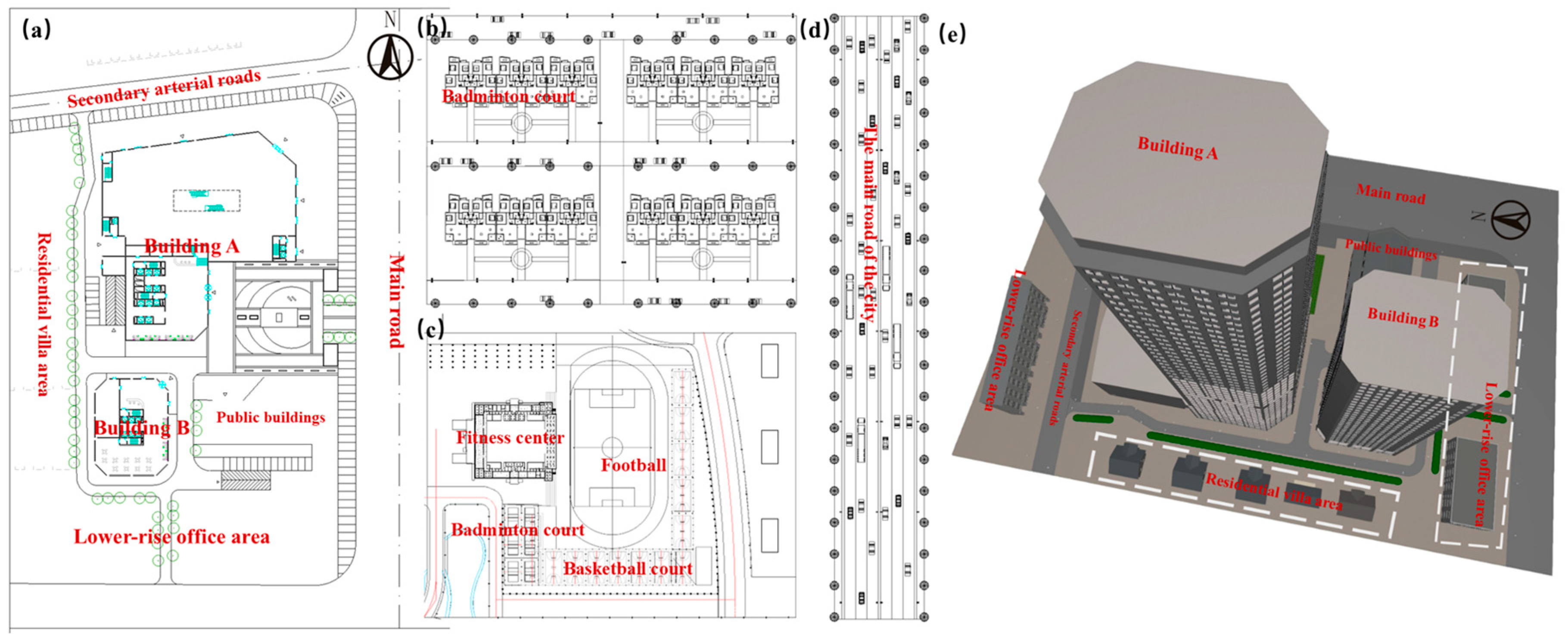
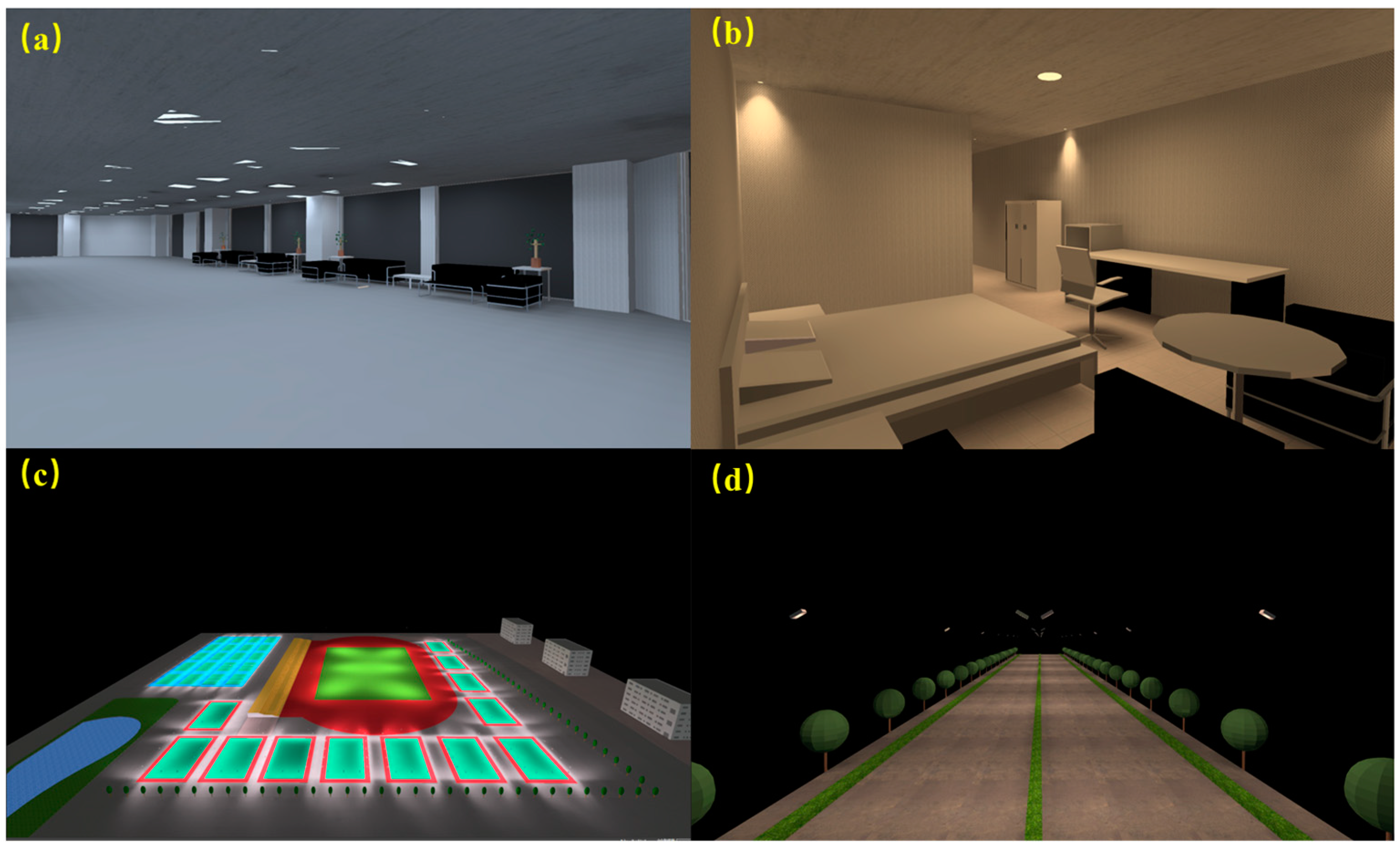
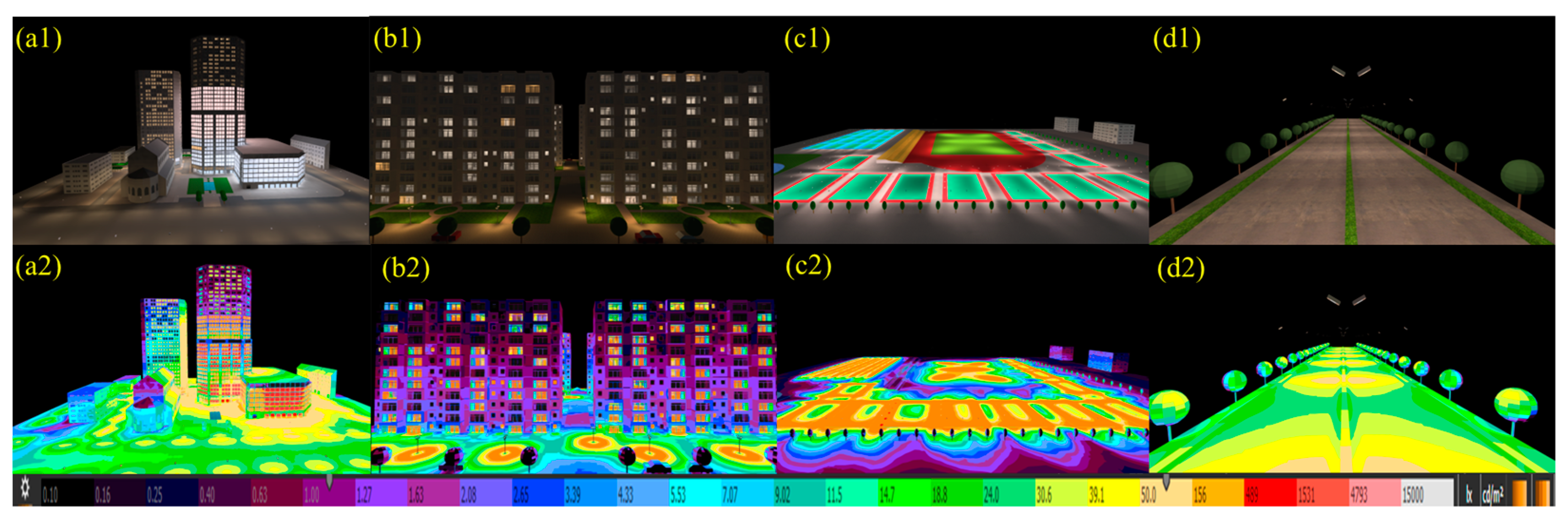
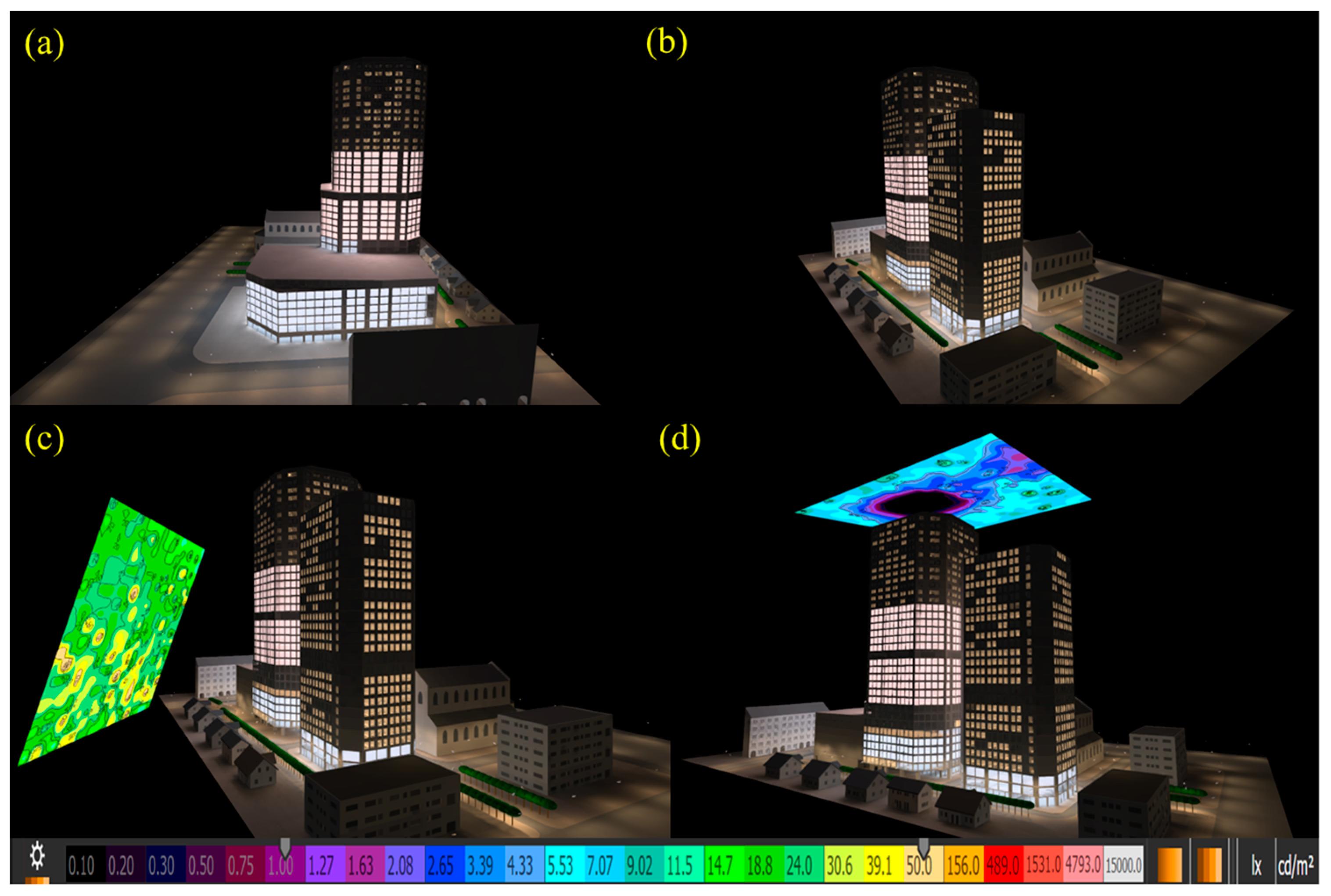
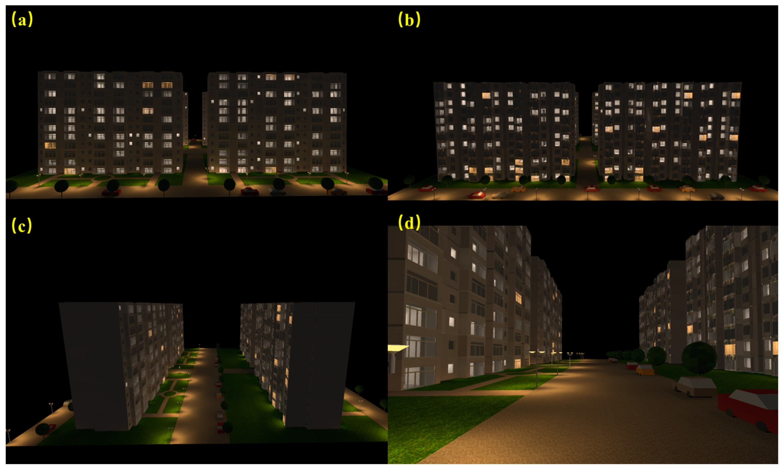
In this study, we conducted a comparative analysis of the nighttime lighting distribution and illumination characteristics in different urban functional scenes (Figure 6). Through modeling and visual representation of typical functional scenes, we revealed the differences in building density, lighting sources, and light intensity across different areas. In the commercial mixed area (Figure 6(a1,a2)), the buildings vary in height, predominantly consisting of mid- to high-rise structures, with a compact layout; the lighting is dense and intense, with significant decorative and advertising lighting on building facades, billboards, and shop windows. The lighting in this area exhibits a strong vertical distribution pattern. In residential areas (Figure 6(b1,b2)), nighttime illumination primarily comes from residential windows and street lighting within the community, with moderate brightness. However, the lighting is mainly concentrated on the front and back facades of buildings and the lower floors. Residential buildings are mostly mid- to low-rise, with relatively even spatial distribution and larger inter-building distances. In the sports park (Figure 6(c1,c2)), there are large open spaces with sports facilities and fields and low-rise buildings, and the ground geometry mostly consists of expansive areas. The intensity and distribution of lighting in these areas vary significantly depending on the use of the space, with a high lighting intensity around sports fields or facilities and weaker lighting in other areas. The main city roads (Figure 6(d1,d2)) are typically wide, with a long linear form, featuring median strips and green belts on both sides of the road. Streetlights with relatively high light intensities are evenly distributed along the main road, with the lighting concentrated on the road surface and within a few meters of it, while areas farther from the road are relatively dim. Therefore, significant differences exist in the nighttime lighting distribution characteristics of different urban functional scenes, primarily in terms of the building density, functional needs, light sources, and light intensity. These differences not only reflect the geometric ground characteristics of the functional areas but also demonstrate their unique nighttime lighting requirements and distributions, providing data and model support for the subsequent analysis of the anisotropy of urban nighttime lighting.

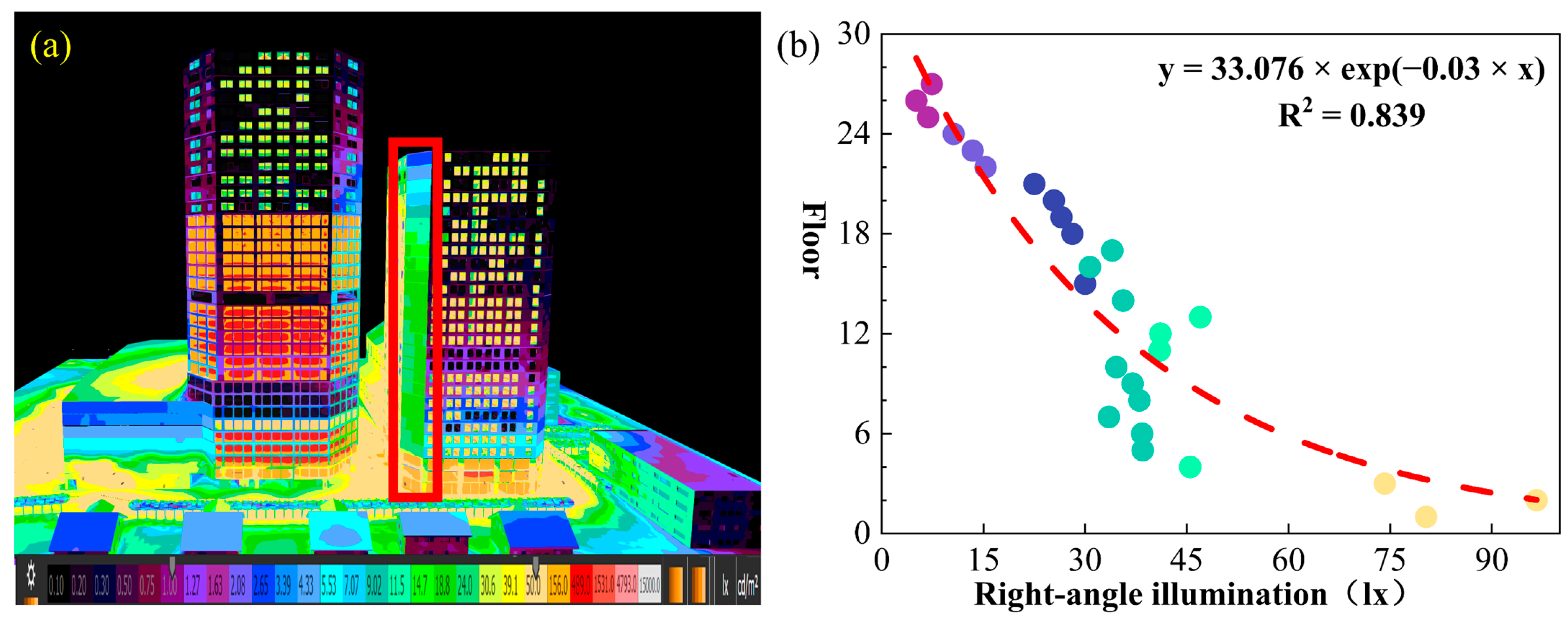
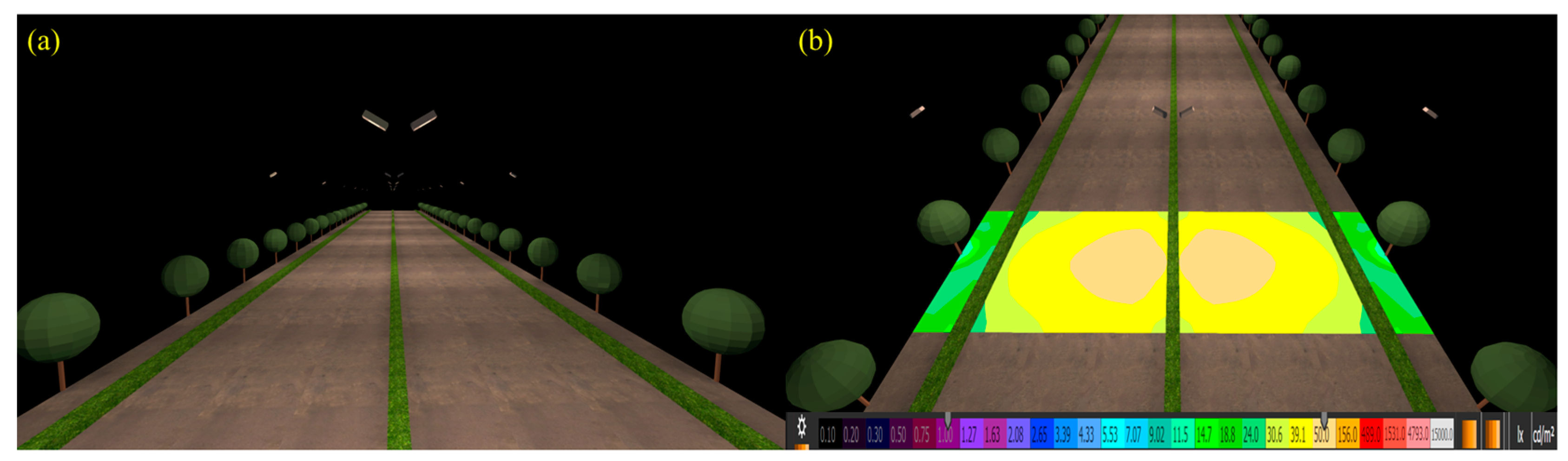
Figure 7 shows the right-angle illuminance distribution of the windowless side facade of building B in the virtual scene of the commercial mixed area and its changes with the floor height. Figure 7a is a pseudo-color image of the side facade of the building, which shows the light intensity in different areas through color changes. Among them, warm colors (such as orange) represent higher illumination areas, while cold colors (such as green and blue) represent lower illumination areas. As shown in the scatter plot and fitting curve in Figure 7b, the illumination at the bottom of the building is higher, and the right-angle illuminance shows a significant exponential decay trend as the number of floors increases. This distribution feature reflects that the lights in the commercial mixed area are usually concentrated in the ground floor area to enhance the brightness of the ground and the surrounding environment, while also improving the business atmosphere.

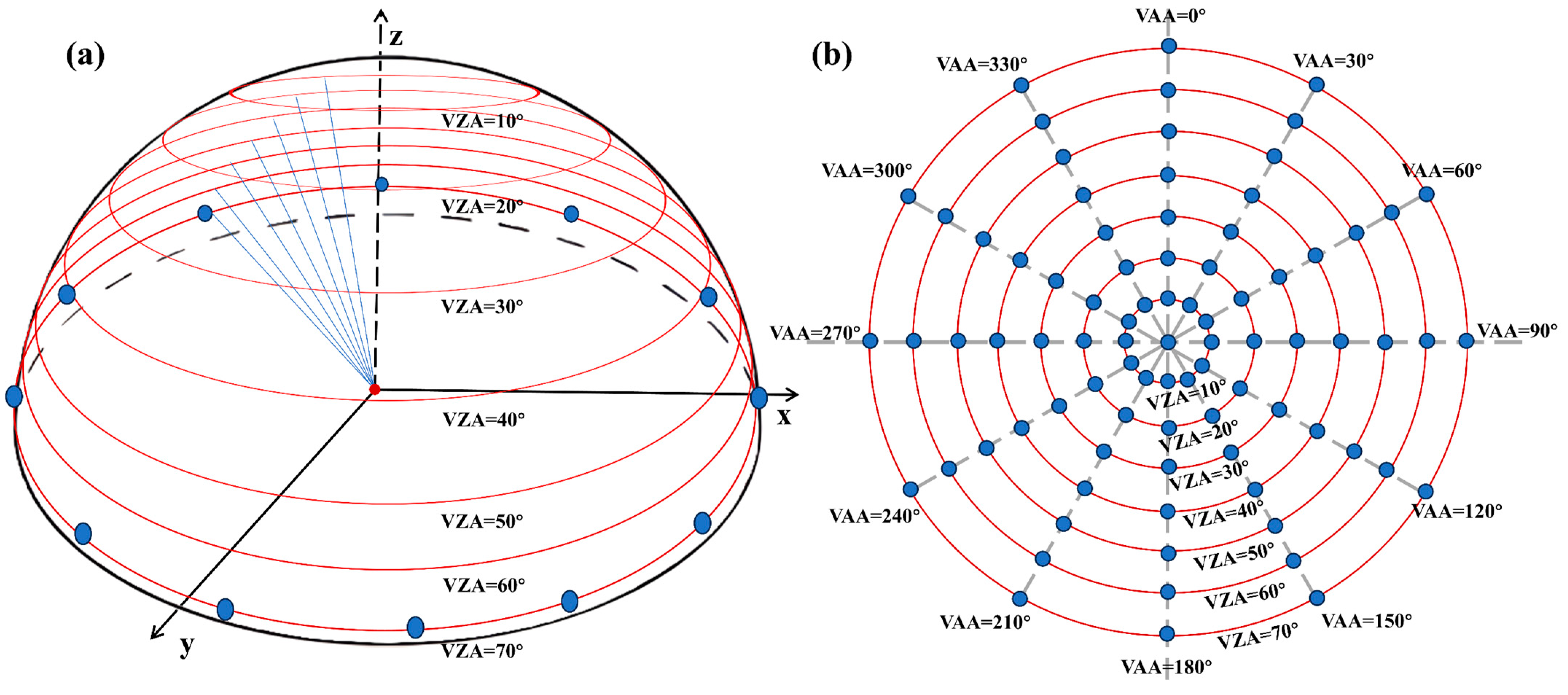
3.2. Relationship Between Zenith Angle, Azimuth Angle, and Right-Angle Illumination in Different Functional Areas

From the combined analysis of the zenith and azimuth observation angles, the nighttime lighting observations in most azimuth directions across the four scenarios exhibited a linear or exponential increase with increasing zenith angle. This phenomenon was likely caused by the diffusion of near-ground light sources and the effects of ground reflection. The variation of nighttime lighting observations with zenith angle was most pronounced in the commercial mixed-use area and urban arterial roads, with the models showing good fitting performances. In the commercial mixed-use area, the vertical distribution of lighting was uniform, with light reflecting off building facades and the ground, resulting in a wide scattered light distribution. The observations at smaller zenith angles showed relatively low values, but as the zenith angle increased, the projection range of the light expanded, leading to a gradual increase in the observation values. For the urban arterial roads and sports park, where the terrain is open, the lighting was evenly distributed, and there were no building obstructions. This resulted in an increasing trend in nighttime illuminance values with zenith angle.

Although the relationship between the zenith angle and nighttime lighting o illuminance values followed a relatively consistent pattern across the scenarios, the relationship between the azimuth angle and illuminance values was more complex. In some scenarios, particularly residential areas and urban arterial roads, the azimuthal variation significantly affected the nighttime illuminance and did not conform well to quadratic regression models. In residential areas, the building layout is orderly, and there is no lighting on the sides of buildings. In certain azimuth directions, building obstructions led to significantly reduced values, while other directions exhibited higher values. This complex lighting distribution makes it difficult to fit the illuminance variations using a simple quadratic model. For urban arterial roads, lighting is predominantly dependent on fixed light sources along the road edges. The distribution and density of these light sources heavily influenced the illuminance values. In some azimuth directions, the extended propagation path of light resulted in higher attenuation rates, leading to a poorer model fit. Overall, the variations in nighttime lighting values with the zenith and azimuth angles were significantly influenced by the urban surface geometry and lighting distribution. While the trends in the lighting values exhibited strong regularity across different urban functional zones, differences in terrain, building layout, and light source distribution led to varying fitting performances across the different scenarios.

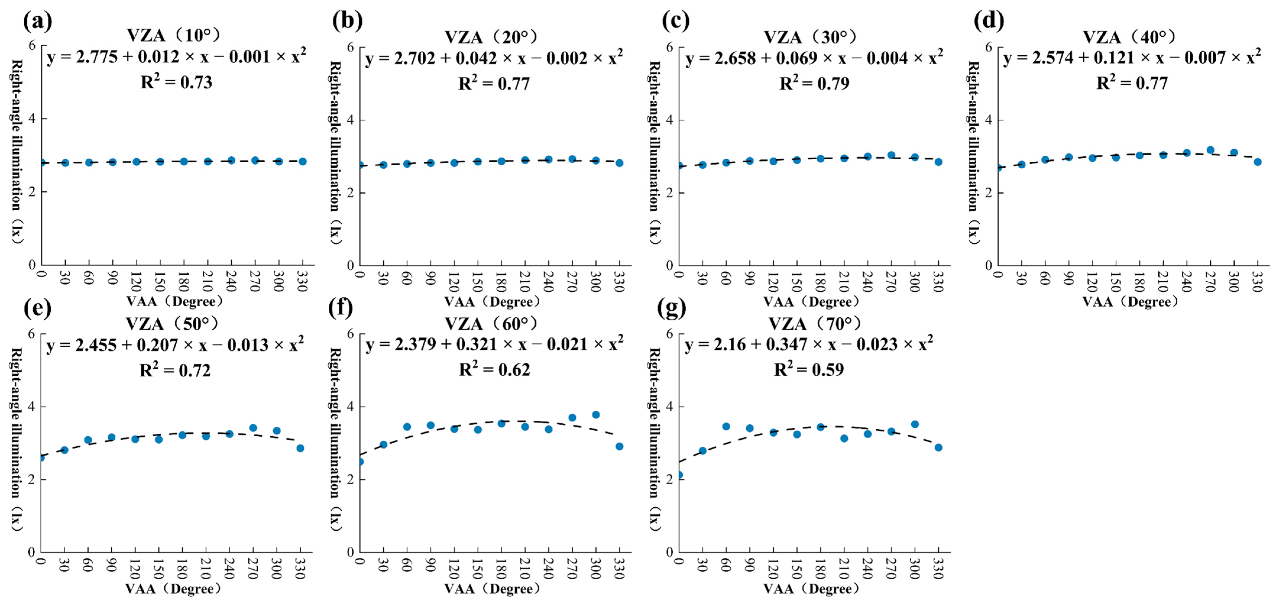
3.2.1. Commercial Mixed Area

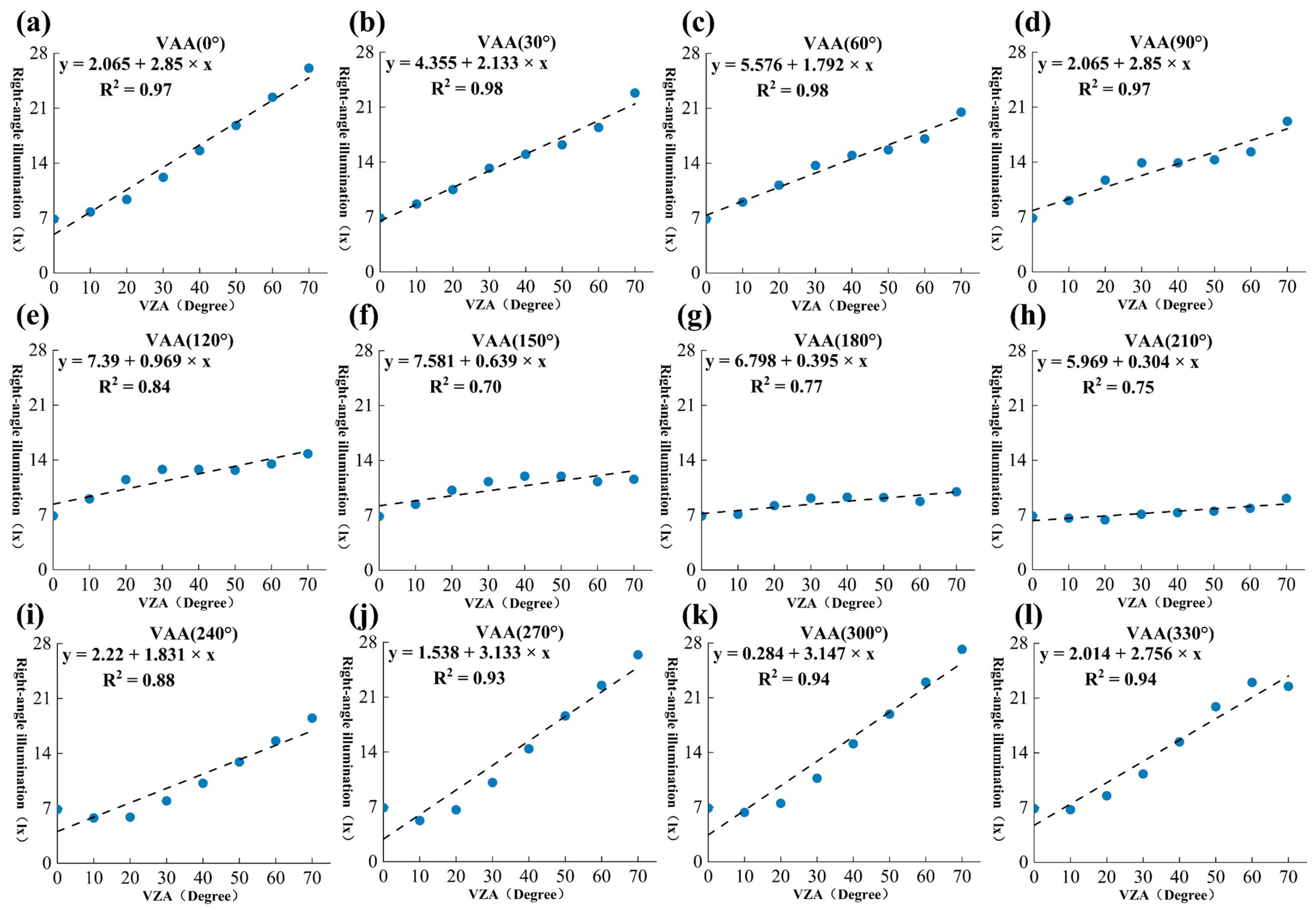
In the study of the anisotropy of nighttime illuminance in the commercial mixed area, the ZIL model was employed to fit the relationship between right-angle illuminance (RAI) and VZA. As shown in Figure 8, overall, the RAI values in the commercial mixed-use area exhibited similar scatter distributions with respect to the VZA. The RAI increased with the VZA, and significant variations were observed in the RAI–VZA relationship across different azimuth angles. For azimuth angles of 0°, 30°, 60°, 90°, 240°, 270°, 300°, and 330°, there was a strong linear correlation between the RAI and VZA, with a good model fitting performance. As illustrated in Figure 9a, the 0° direction corresponds to the maximum illuminance. In this direction, the light sources are concentrated, and the light encounters minimal obstruction from buildings. In particular, at high zenith angles, the light more directly illuminated the calculation plane, leading to a notable increase in illuminance with the VZA. Conversely, for azimuth angles of 120°, 150°, 180°, and 210°, the changes in the RAI were more gradual, and the linear correlation was weaker. This indicates a more uniform light distribution in these directions, with less pronounced anisotropic effects. As shown in Figure 9b, the 210° direction corresponds to the minimum illuminance. In this direction, the shape and arrangement of the buildings are more complex, causing greater light obstruction. This resulted in more uniform and diffused lighting, where the light could not directly reach the calculation plane, leading to smaller variations in the RAI with the VZA.

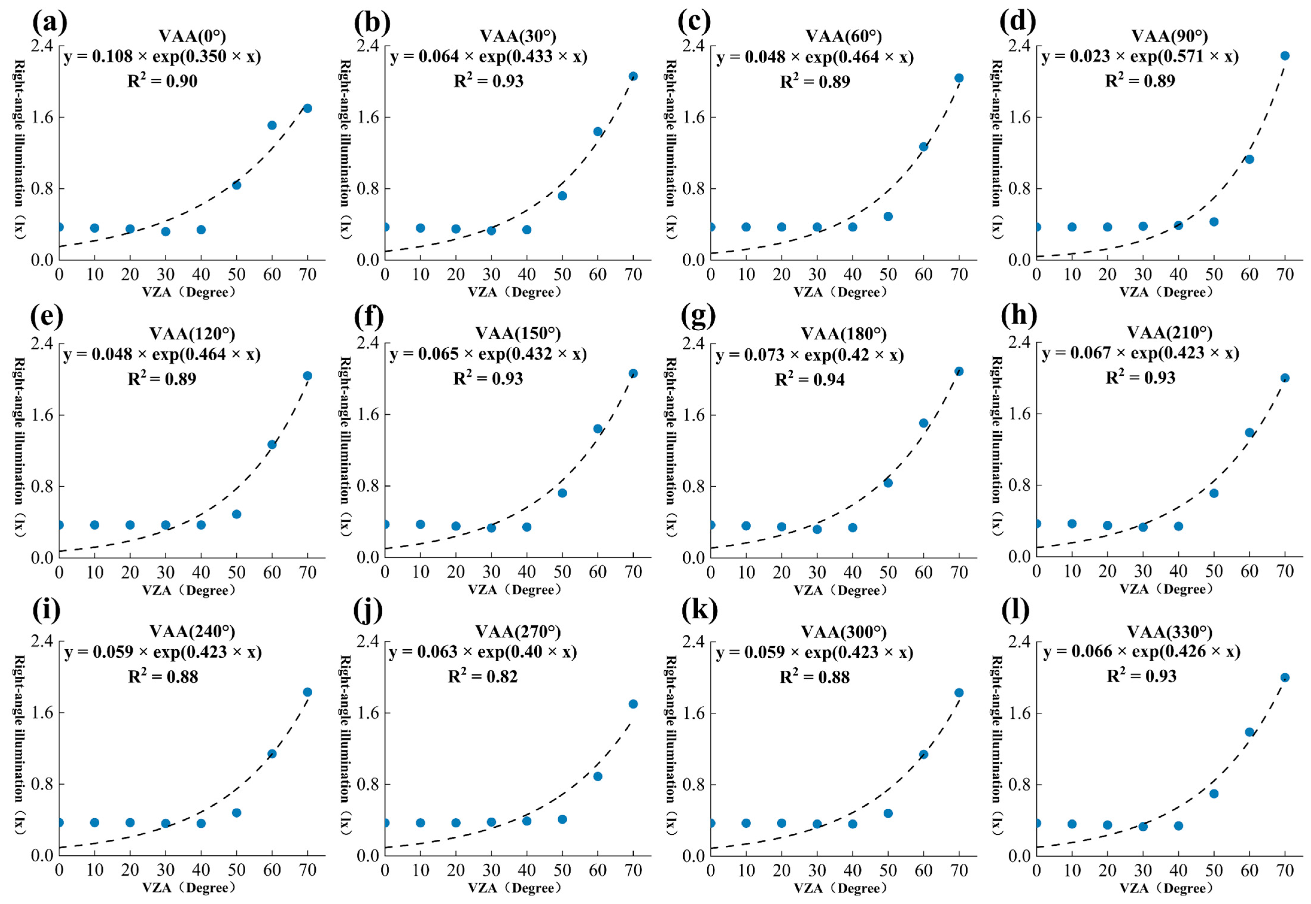
In this study, the AIQ model was utilized to fit the relationship between right-angle illuminance (RAI) and VAA, with the results shown in Figure 10. In the commercial mixed-use area, the overall RAI variation exhibited a clear U-shaped distribution with increasing VAA. Specifically, the illuminance was weaker near 210°, while it peaked near 0°, particularly when the VZA was 50° or higher. In these cases, the correlation between RAI and VAA was strong, and the quadratic regression curve showed a better fitting performance. At smaller VZA values, such as 20° and 30°, the RAI variation with VAA was more gradual, with weaker correlations. This behavior was influenced by the distribution of building lighting and observation angles in the commercial mixed-use area. At higher zenith angles (Figure 9c), the view became more horizontal, making the asymmetric distribution of light sources more pronounced, leading to significant illuminance variations with VAA. Conversely, at lower zenith angles (Figure 9d), the view was more vertical, resulting in smaller differences in nighttime illuminance across different azimuth angles.

3.2.2. Residential Area

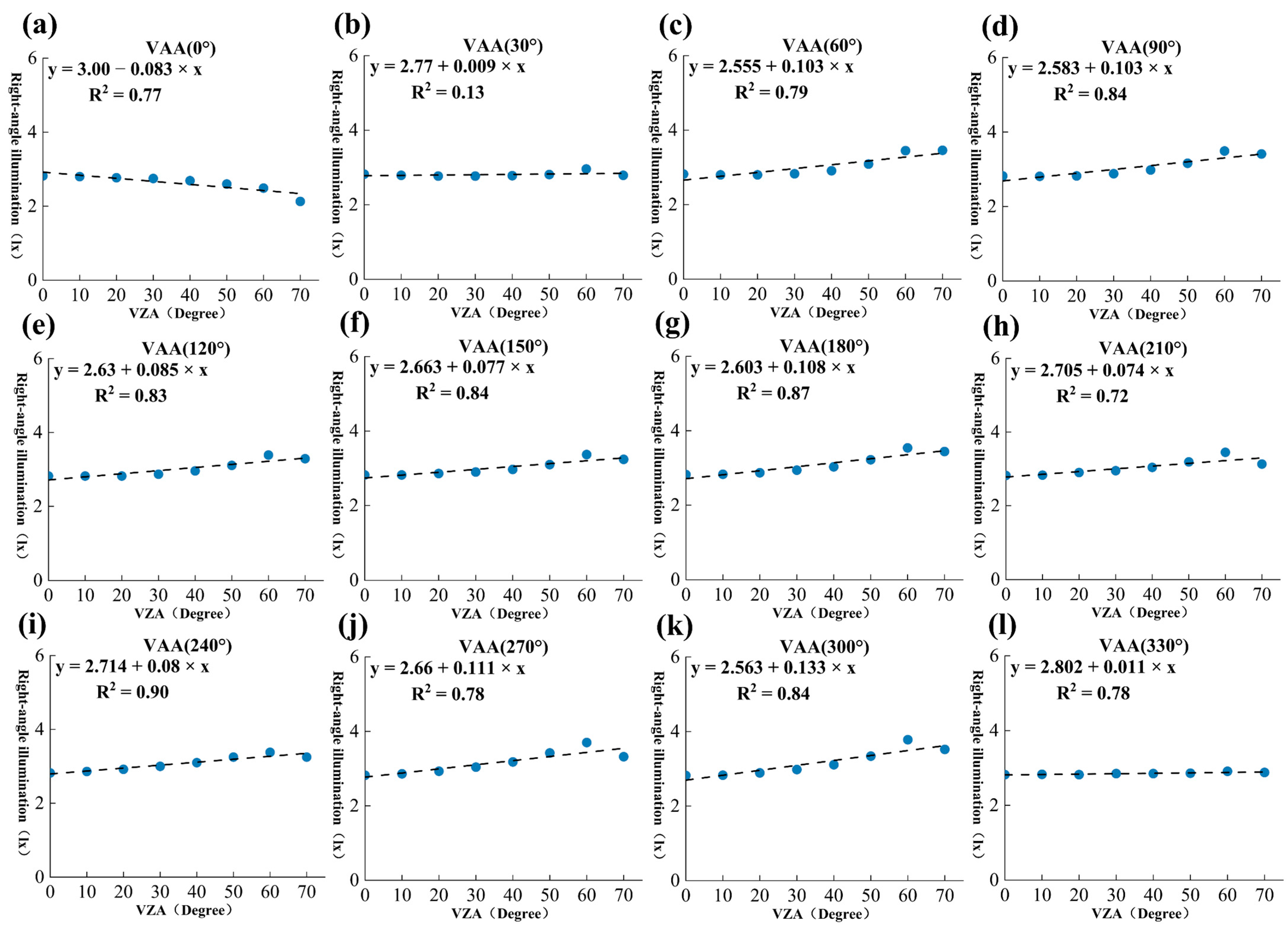
For the study of nighttime illuminance anisotropy in residential areas, the ZIL model was similarly employed to fit the relationship between RAI and VZA. As shown in Figure 11, overall, in most directions, the illuminance intensity increased with the zenith angle, and the model demonstrated a good fit. However, the light distribution in residential areas exhibited certain regularity (Figure 12) in the 90° and 270° directions. Due to the absence of lighting on the two sides of buildings, a significant decreasing trend was observed as the zenith angle increased. In the 60°, 120°, 240°, and 300° directions, the fitted curve showed a smaller slope, indicating that the illuminance values exhibited a slow growth trend or remained nearly constant as the zenith angle increased. This suggests that the above directions were influenced by the shielding effect of the buildings and the distribution of the light sources.

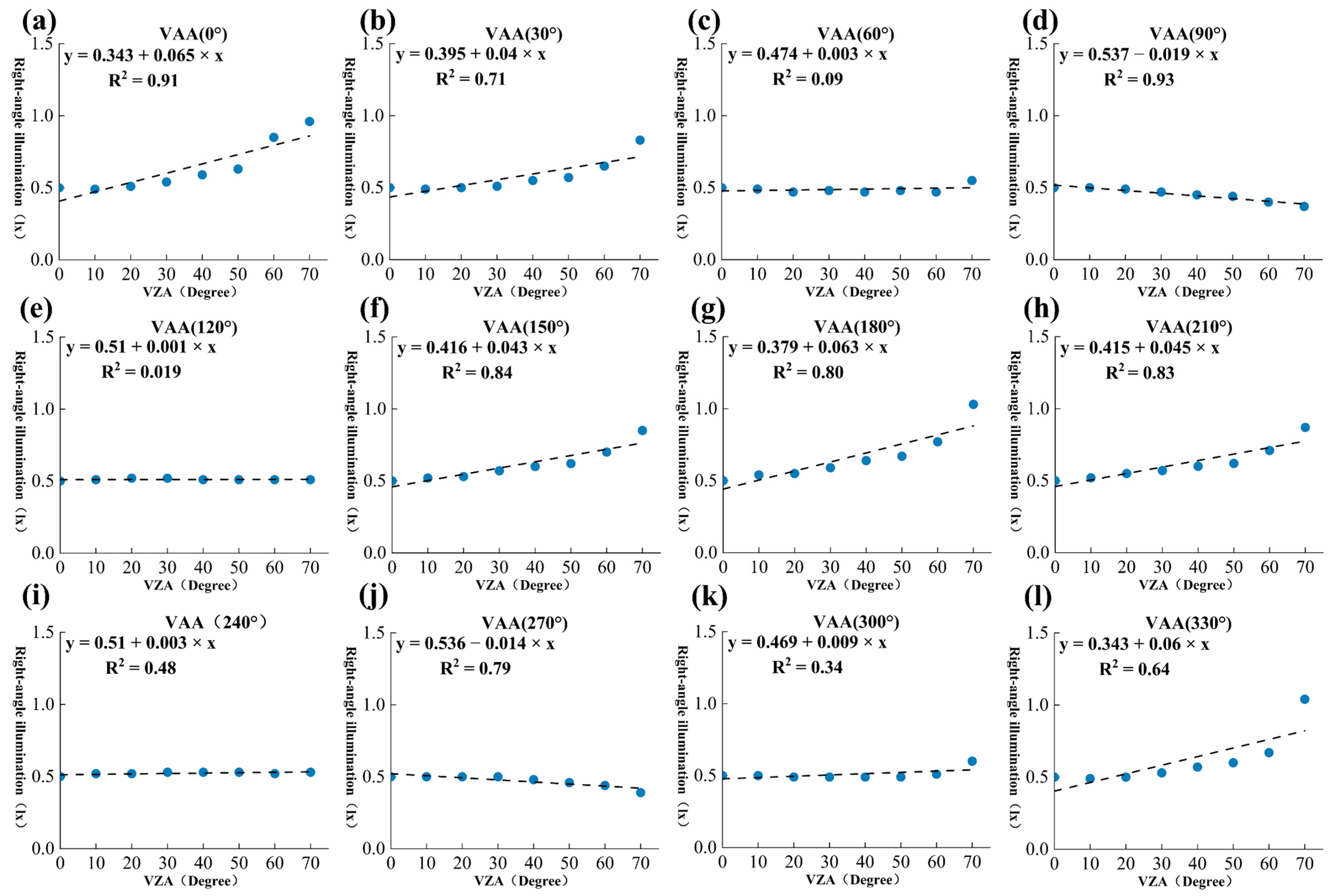
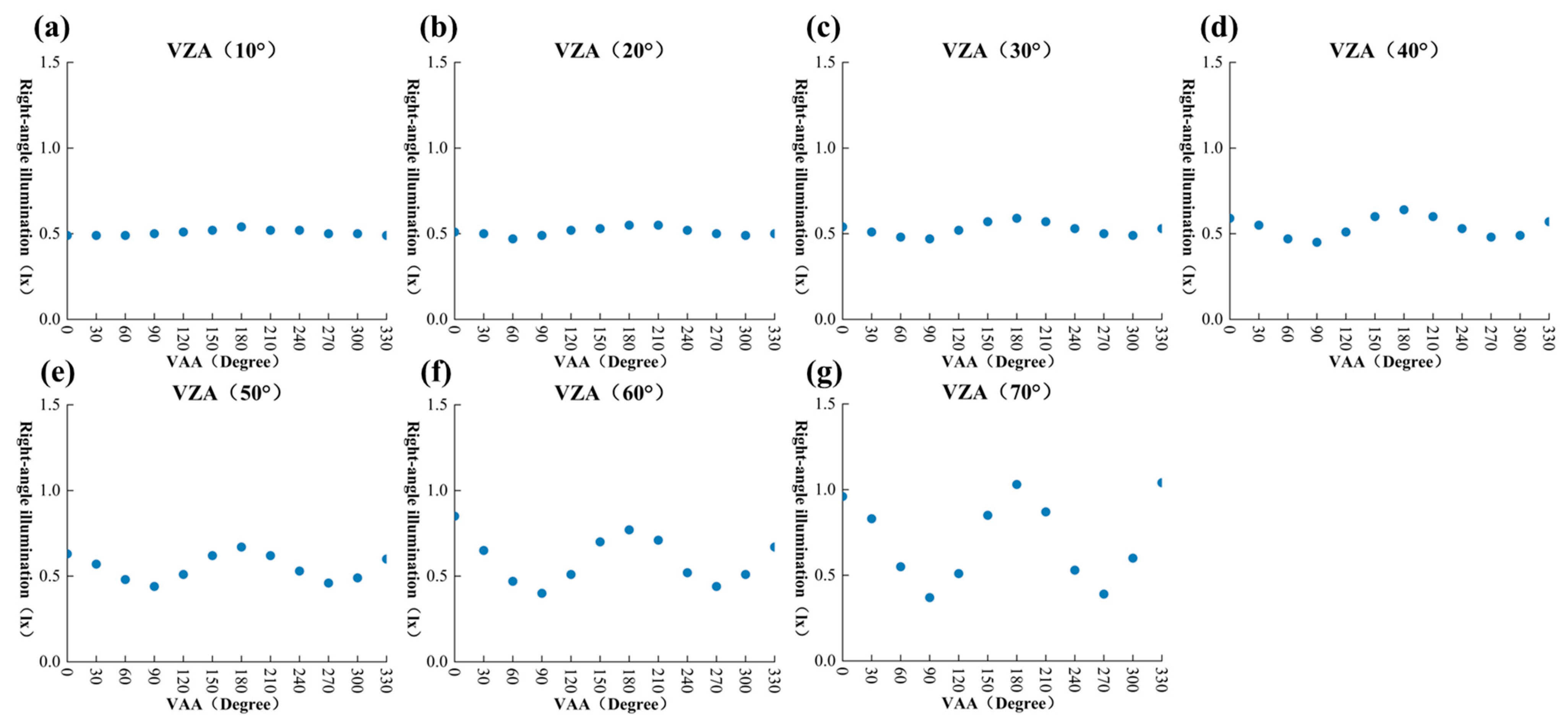
As shown in Figure 13, the AIQ model was used to fit the relationship between the azimuth angle (VAA) and illuminance. At low zenith angles (10–40°), the illuminance intensity across the different azimuth angles remained stable and showed no significant fluctuations. The illuminance values were relatively uniform in all directions, ranging from approximately 0.4 to 0.6 lx. This indicates that, at low zenith angles, the light primarily from horizontal or near-horizontal light sources, was minimally obstructed and relatively evenly distributed in all directions. At zenith angles of 50° and 60°, the illuminance values in the different azimuth directions began to show noticeable fluctuations as the zenith angle increased. In particular, at a zenith angle of 60°, the variations were more pronounced, with the maximum illuminance reaching 0.8 lx and the minimum being around 0.4 lx. These fluctuations were caused by partial obstruction of the light sources in some azimuth directions and the lack of lighting distribution on the sides of residential buildings, leading to uneven illumination (Figure 12c). At a high zenith angle of 70°, the fluctuations in illuminance became even more significant, with the intensity ranging between 0.4 and 1.2 lx. The effects of the building obstructions and lighting distribution were further amplified at this zenith angle, resulting in pronounced azimuthal anisotropy.

3.2.3. Sports Park

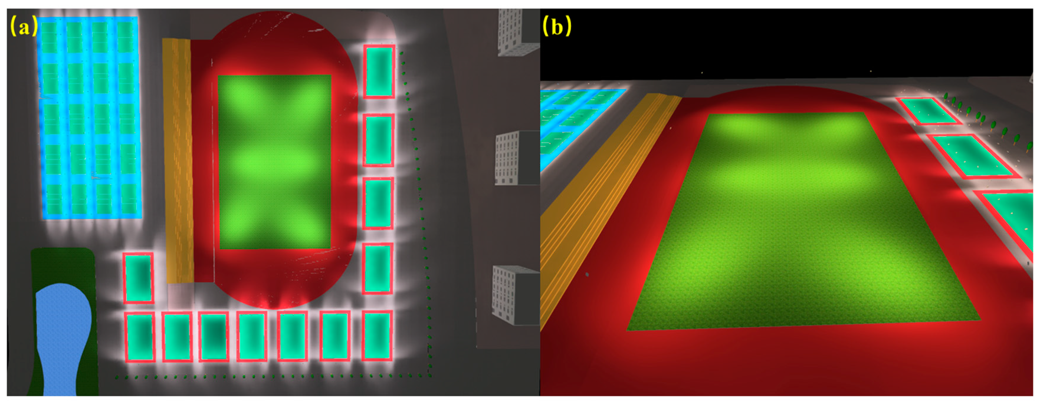
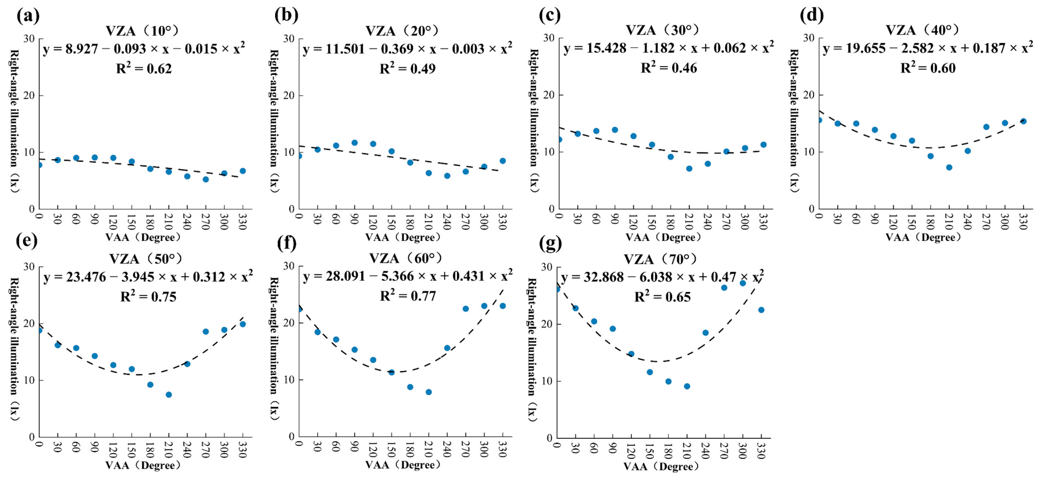
For the sports park, the ZIL model was similarly employed to fit the relationship between the zenith angle (VZA) and illuminance. As shown in Figure 14, in most azimuth directions, the illuminance intensity exhibited a linear growth trend. The illuminance intensity decreased with increasing zenith angle in the 0° direction. Based on the lighting distribution of the scene (Figure 15b), this may be due to the relatively open area with sparse light sources in this direction. In the 60–300° range, the illuminance intensity varied significantly with zenith angle, which is related to the concentrated distribution of lighting around the sports field. Variations in illuminance intensity in the different directions may be influenced by the distribution of lights, the field design, and other factors.

As shown in Figure 16, the variations in rectangular illuminance within the sports park exhibited a parabolic trend, first increasing and then decreasing across the different zenith angles (VZAs). This trend became more pronounced as the zenith angle increased. When the VZA was 60° or 70°, the light projection direction was nearly perpendicular to the main activity areas, resulting in higher illuminance values. This was due to the combined effects of the concentrated light projection and ground reflection in these directions, producing prominent illuminance peaks. In the fitted curves for the various zenith angles, the illuminance peaks were predominantly observed at azimuth angles of 60° and 300°. Beyond an azimuth of 60°, the illuminance values started to decrease. This pattern aligns with the typical lighting arrangement in the sports park, which is characterized by large, uniformly illuminated areas (Figure 15a). The open ground morphology further contributed to the uniform distribution of light, leading to consistent illuminance across different azimuth angles without significant unevenness or sharp decreases.

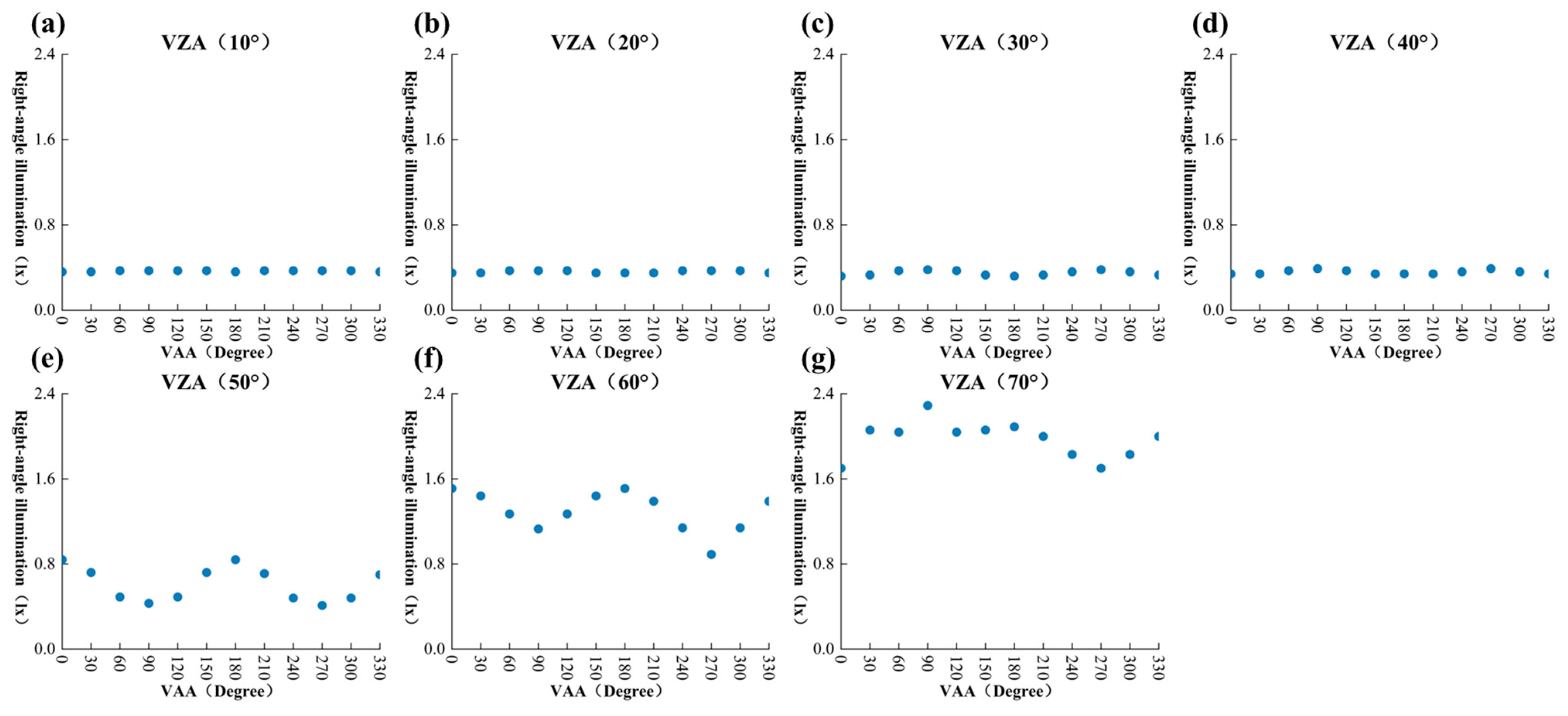
3.2.4. Main City Roads

In the urban arterial road scenario, the ZIE model was employed to fit the relationship between the zenith angle (VZA) and nocturnal illuminance under different azimuth angles. As shown in Figure 17, the rectangular illuminance values at all azimuth angles exhibited exponential growth with increasing VZA, with R² values exceeding 0.8, indicating a strong model fit. At lower zenith angles (0–40°), the illuminance values changed minimally, whereas at zenith angles between 50° and 70°, the illuminance demonstrated a marked stepwise increase. This pattern is closely related to the lighting distribution of urban arterial roads, as illustrated in Figure 18a. The light sources primarily consist of streetlights located along both sides and in the center of the road, designed to illuminate the roadway. At larger zenith angles, the observational perspective became more vertical, allowing more light to reach the observation plane and resulting in higher illuminance values.

As shown in Figure 19, in the urban arterial road scenario, the illuminance distribution across different azimuth angles was uniform at low zenith angles, with minimal fluctuations and no significant variation. The azimuth angle differences had little impact on the illuminance distribution at these angles. However, as the zenith angle increased, the illuminance values rose. Due to the relatively uniform emission angles of the light sources, direct light received by the observation plane from the sources decreased in certain azimuth angles, resulting in slight variations in the illuminance values. Urban arterial roads are typically wide, with flat surfaces, and the lighting is primarily arranged along both sides and in the center of the road, utilizing directional light sources. This layout creates a relatively uniform distribution of illuminance across the central and side areas (Figure 18b). Such symmetrical lighting distribution is a key objective in modern road design, as it ensures traffic safety and significantly enhances nighttime road visibility.

3.3. Comparative Analysis of Anisotropy of Night Light Emission in Different Functional Areas of a City

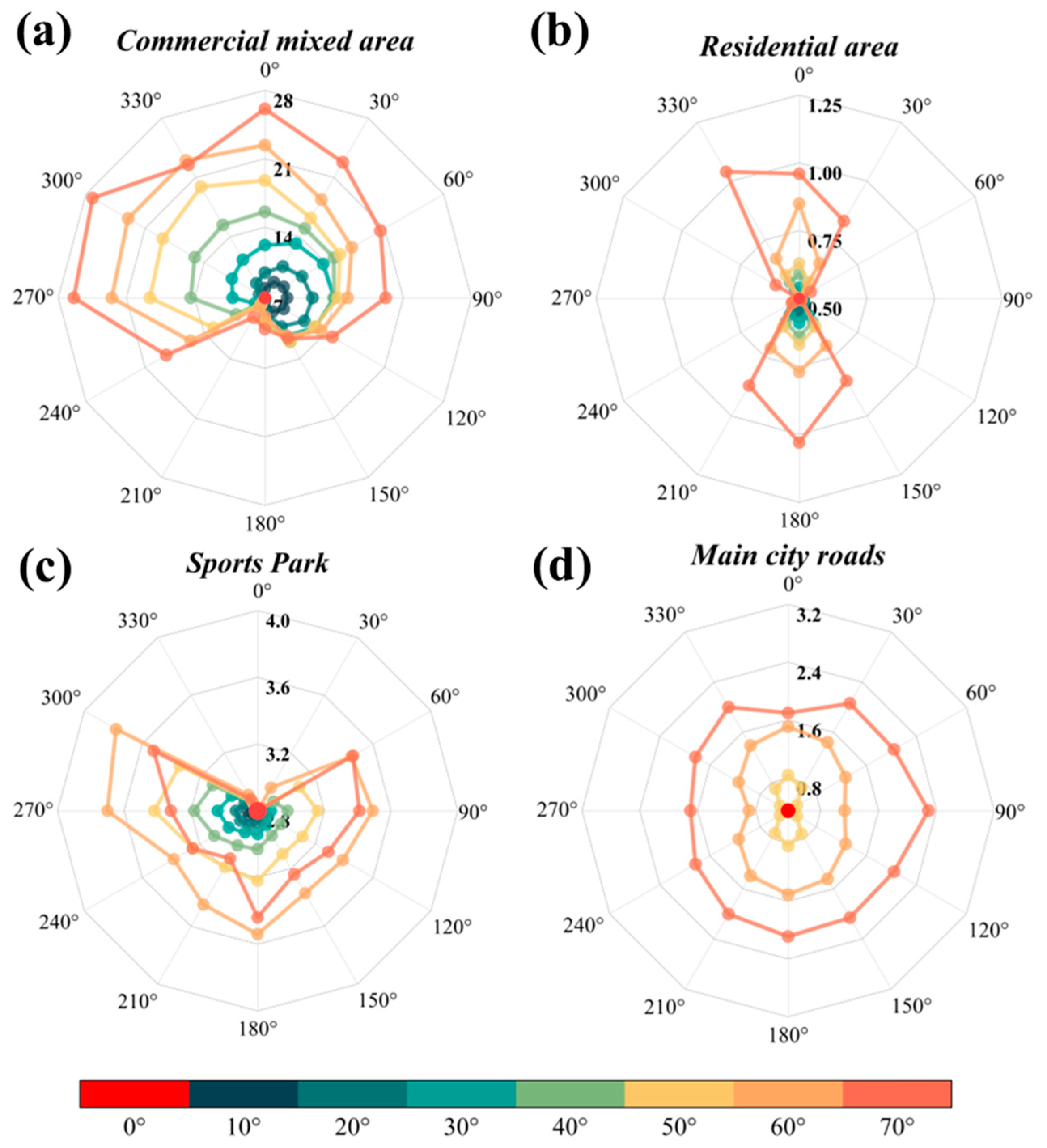
As shown in Figure 20, in most directions in the different functional scenarios, the relationship between the nighttime illuminance values and observation zenith angles followed a consistent pattern: as the observation zenith angle increased, the nighttime illuminance values also increased. Additionally, the intensity of nighttime lighting in different functional scenarios exhibited distinct angular distribution characteristics. In the commercial mixed-use area (Figure 20a), the illuminance at all angles was relatively high, and with an increase in zenith angle, the lighting intensity significantly increased, with the maximum illuminance distributed at high zenith angles (VZA of 70°), reaching approximately 28 lx. This indicates that the illuminance of the commercial mixed-use area is influenced by the obstruction of high-rise buildings and dense lighting, resulting in a clear directional distribution of nighttime lighting intensity. In residential areas (Figure 20b), the illuminance distribution was relatively uniform, with overall lower lighting levels, peaking at around 1 lx. However, it exhibited high symmetry, with the front and back of residential buildings having higher illuminance, while the sides had lower values. In the sports park (Figure 20c), the lighting intensity showed clear directionality, particularly at high zenith angles in the 60° and 300° directions, where the maximum value reached approximately 3.8 lx. This suggests that the lighting facilities in the sports park are likely concentrated in specific directions to focus lighting on certain sports areas. In the urban arterial roads (Figure 20d), the lighting intensity changed symmetrically with the azimuth angle, with a maximum value of 2.31 lx at the 90° azimuth angle. The overall lighting in the urban arterial roads was relatively low but symmetrical, indicating an even distribution of lighting facilities along the sides of the roads.

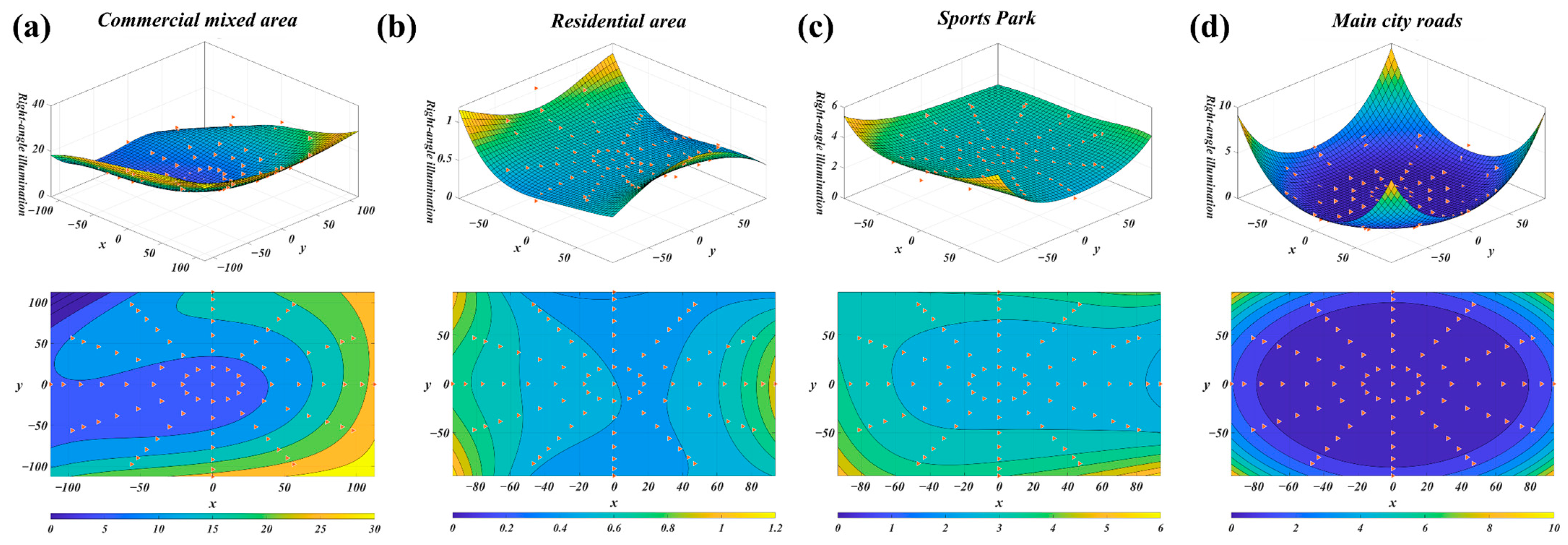
In this study, we constructed the AZIP model and proposed a polynomial regression-based surface fitting method. Using the least squares method, we fit the nighttime rectangular illuminance surfaces for various functional scenes, generating 3D nighttime illuminance distribution maps and contour plots. These visualizations effectively display the angular variation characteristics of nighttime lighting.

As shown in Figure 21, the directional characteristics of nighttime illuminance differed across the four functional scenes. In the commercial mixed-use area, the primary lighting sources are concentrated in two major buildings at the center of the scene, with extensive illumination distributed across many buildings. The fitted surface (Figure 21a) showed strong central symmetry in its illuminance distribution. The contour lines were roughly concentric, indicating relatively uniform lighting in this area. However, due to obstructions from buildings at the 180° and 210° directions, the calculated illuminance values were lower, showcasing its anisotropic characteristics. In the residential area, the illuminance distribution exhibited clear symmetry. The fitted surface (Figure 21b) showed higher illuminance values at the sides of the scene, gradually decreasing toward the center. This is related to the uneven distribution of light from window transmissions and exterior wall lights in the residential buildings. The contour map showed a gentler change in illuminance, indicating a generally lower illuminance, consistent with the characteristics of nighttime lighting in residential areas. The sports park features a large, flat ground geometry with a lighting design primarily based on local lighting. Focused lighting is arranged around different sports areas, resulting in significant fluctuations in the illuminance distribution. The fitted surface (Figure 21c) showed large variations in high and low illuminance values, with peak illuminance occurring at the edges or in specific areas of the scene. The contour map also exhibited an irregular distribution, reflecting the variation in lighting around the park. The fitted surface for the urban main road (Figure 21d) displayed a bimodal structure with low illuminance in the center and higher illuminance on the sides, indicating that the lighting along the road was concentrated along the two sides. The road has a wide and uniform lighting range, and as a result, the contour map showed a symmetrical elongated elliptical distribution on both sides.

In conclusion, the anisotropy of nighttime lighting in the four scenes is significantly influenced by the ground geometry and lighting distribution. The illuminance distributions in the commercial mixed-use area and the urban main road were relatively uniform and symmetric, with lighting concentrated in specific areas, although they differed in their layout. The commercial mixed-use area, driven by the high lighting demand of commercial activities, has dense and concentrated lighting arranged in the buildings, with the primary light sources being the transmitted light from commercial building windows. In contrast, the urban main road requires high-intensity and uniform lighting to ensure safety, resulting in symmetric streetlight arrangements along both sides of the road. The residential area and sports park emphasize local lighting, showing clear gradients in illuminance, with relatively gentle transitions in lighting. These two areas are more influenced by lighting demands and the light distribution.

4. Discussion

4.1. Relationship Between Nighttime Light Anisotropy and Urban Geometry

In analyzing the nighttime lighting anisotropy of four typical urban functional scenes—a commercial mixed-use area, residential area, sports park, and urban main roads—the ground geometry and building layout were found to have a significant impact on the spatial distribution and anisotropy of the nighttime lighting. In scenes with dense buildings and significant height differences (such as the commercial mixed area), multiple reflections and obstructions of light enhanced the uneven distribution of illumination, both vertically and horizontally. This was especially noticeable at higher zenith angles, where the illuminance values varied significantly with the azimuth angle. Factors like building facade materials and glass curtain walls further intensified the light’s multi-angle reflection and refraction effects. On the other hand, areas with shorter and more widely spaced buildings tended to exhibit a relatively uniform lighting distribution, though localized strong light spots still appeared due to the concentration of light sources in certain regions.

In the residential area, which consisted of low-rise or mid-rise buildings with regular layouts and larger distances between structures, the lighting distribution was relatively smooth. In the sports park, the terrain is more open, with light sources concentrated around various sports fields, causing rapid illuminance decay with distance. The wide ground surface and the linear distribution of light sources along the urban main roads resulted in concentrated illuminance along the road direction, with limited dispersion to the sides. As a result, there was no obvious anisotropy in terms of azimuth angles; however, anisotropy became apparent as the zenith angle changed. If buildings are present on both sides of the road, more pronounced anisotropic characteristics were observed. In summary, the ground geometry and building layout of urban functional areas are the key factors influencing nighttime lighting anisotropy. Dense, compact building layouts and varying building heights intensify the anisotropy in such regions.

4.2. Relationship Between Nighttime Light Anisotropy and Light Distribution

In this study, we also observed a significant relationship between the lighting distribution characteristics of the various functional zones and the nighttime lighting anisotropy. The design of the lighting, source placement, and the way the light propagates jointly determine the spatial distribution of illuminance. These characteristics play a crucial role in the variation in lighting intensity under different spatial observation angles. In the commercial mixed area, the nighttime lighting mainly comprises high-intensity commercial billboards, streetlights, and glass facades, leading to strong reflections and refractions across multiple directions due to the high density and varying heights of buildings in the region. In this complex lighting environment, the anisotropy of lighting was particularly pronounced, especially at higher zenith angles, where the illuminance varied significantly across the different azimuth angles.

Compared to the commercial mixed-use area, the lighting distribution the residential area was relatively simpler, with light sources mainly coming from streetlights and localized lighting inside residential buildings, resulting in weaker illuminance. The sparse arrangement of buildings led to fewer instances of light obstruction and reflection during propagation. However, due to the uneven distribution of light on the front, back, and sides of the buildings, some anisotropy was still observed. In the sports park, anisotropy mainly resulted from the concentrated distribution of local lighting. The nighttime illumination in these areas primarily comes from high-mounted floodlights, which caused limited horizontal light propagation while exhibiting strong light decay in the vertical direction. Additionally, due to the relatively open nature of the space and the fewer buildings, there were minimal reflections and obstructions of light. In the urban arterial roads, the nighttime lighting mainly comes from streetlights and vehicle headlights, showing a relatively uniform distribution of illuminance. However, the linear arrangement of light sources caused the illumination to concentrate in the center of the road, with the intensity gradually decreasing on the sides, forming a typical anisotropic characteristic. In conclusion, the lighting design and distribution in urban functional areas are critical factors influencing the anisotropy of nighttime lighting. The varying lighting needs of different functional zones lead to distinct anisotropic features in each zone.

4.3. Future Work

This study, through virtual simulation modeling, systematically analyzed the anisotropic characteristics of nighttime lighting in complex urban scenes for the first time. It revealed the combined effects of the zenith angle and azimuth angle on the distribution of nighttime lighting, further emphasizing the key role of the azimuth angle. This contrasts with the existing satellite remote sensing studies, which primarily focused on the impact of the zenith angle on the anisotropy of nighttime lighting. Additionally, this study clarified the mechanisms through which urban geometric forms and light distributions influence anisotropy, providing a theoretical basis for the multi-angle calibration of satellite remote sensing data. Finally, a polynomial regression-based surface fitting method was proposed, offering a new approach for the quantitative study of nighttime light anisotropy. Compared to the existing research, the innovation of this study lies in the integration of virtual simulation technology to construct a three-dimensional model of complex urban scenes, enabling a more realistic simulation of the spatial distribution and anisotropic characteristics of nighttime lighting.

However, there are still some limitations that need to be addressed in future work. First, the cityscape models established in this study are virtual. In future work, it will be essential to integrate field surveys, ground measurement data, and multi-source remote sensing data to create a refined 3D urban lighting model that simulates processes such as light propagation, reflection, and refraction. This will further enhance the understanding of nighttime lighting anisotropy in different urban areas. Second, this study used empirical statistical models to describe anisotropy. Future modeling should integrate ground observation data with ray tracing models, incorporating factors related to the ground geometry, to further explain the relationship between observation angles and nighttime lighting intensity. Finally, by analyzing the anisotropy of nighttime lighting in urban functional areas, future research can focus on the dynamic changes in nighttime lighting. Utilizing smart lighting technologies, it will be possible to dynamically adjust the lighting intensity and distribution in different areas, reducing the impact of anisotropy on the surrounding environment and minimizing unnecessary light pollution. This will contribute to the goals of conserving energy and protecting the environment.

5. Conclusions

Anisotropic reflection characteristics are a well-known phenomenon in remote sensing, while the anisotropy of nighttime lighting remains a significant challenge in nighttime light remote sensing research. This study investigated the anisotropy of nighttime lighting by establishing a simulation model for complex urban nighttime lighting scenes. The results show that the illuminance distribution in functional areas is uneven, with nocturnal illuminance values exhibiting linear or exponential variations with zenith angle and quadratic variations with azimuth angle. In some functional areas, the illuminance distribution is uniform, without significant anisotropy. By using a polynomial-based fitting method, we plotted nocturnal illuminance surfaces for different urban functional scenes, revealing that the anisotropy of nighttime lighting varies across functional areas. This demonstrates that the anisotropy of nighttime lighting is closely related to the geometric form of the urban scene and the distribution of lighting.

This study demonstrated that the anisotropy of nighttime lighting is not only influenced by the zenith angle, but also by the observation azimuth angle, offering a better explanation of the relationship between the zenith angle, the azimuth angle, and nocturnal illuminance. It also revealed the impact of ground geometric forms and light distributions on the anisotropy of nighttime lighting. This finding deepens the understanding of the transmission mechanisms of nighttime light and provides theoretical support for mitigating the effects of anisotropy on nighttime light data, resulting in more stable and accurate nighttime light data that can more effectively reflect social dynamics. Furthermore, this study provides a scientific basis for urban lighting design, helping to reduce urban light pollution and ensuring the sustainable development of residents’ quality of life and the ecological environment. It should be noted that, due to the complexity of urban functional area lighting environments, the modeling was based on representative buildings from each functional area, and the results may not fully capture the lighting characteristics of the entire functional area. Future research could expand the sample range by incorporating a more diverse range of building types and spatial layouts to more comprehensively reveal the anisotropic patterns of nighttime lighting.

References

1. Kyba, C.C.M.; Kuester, T.; Sánchez de Miguel, A.; Baugh, K.; Jechow, A.; Hölker, F.; Bennie, J.; Elvidge, C.D.; Gaston, K.J.; Guanter, L. Artificially lit surface of Earth at night increasing in radiance and extent. Sci. Adv. 2017, 3, e1701528. [Google Scholar] [CrossRef]
2. Mason, I.C.; Grimaldi, D.; Reid, K.J.; Warlick, C.D.; Malkani, R.G.; Abbott, S.M.; Zee, P.C. Light exposure during sleep impairs cardiometabolic function. Proc. Natl. Acad. Sci. USA 2022, 119, e2113290119. [Google Scholar] [CrossRef] [PubMed]
3. Moore, M.V.; Pierce, S.M.; Walsh, H.M.; Kvalvik, S.K.; Lim, J.D. Urban light pollution alters the diel vertical migration of Daphnia. Int. Ver. Für Theor. Angew. Limnol. Verhandlungen 2000, 27, 779–782. [Google Scholar] [CrossRef]
4. Owens, A.C.S.; Cochard, P.; Durrant, J.; Farnworth, B.; Perkin, E.K.; Seymoure, B. Light pollution is a driver of insect declines. Biol. Conserv. 2020, 241, 108259. [Google Scholar] [CrossRef]
5. Korner, P.; von Maravic, I.; Haupt, H. Birds and the ‘Post Tower’ in Bonn: A case study of light pollution. J. Ornithol. 2022, 163, 827–841. [Google Scholar] [CrossRef]
6. Falchi, F.; Cinzano, P.; Duriscoe, D.; Kyba, C.C.M.; Elvidge, C.D.; Baugh, K.; Portnov, B.A.; Rybnikova, N.A.; Furgoni, R. The new world atlas of artificial night sky brightness. Sci. Adv. 2016, 2, e1600377. [Google Scholar] [CrossRef] [PubMed]
7. Walker, M.F. Light Pollution in California and Arizona. Publ. Astron. Soc. Pac. 1973, 85, 508. [Google Scholar] [CrossRef]
8. Bertiau, F.C.; Graeve, E.d.; Treanor, P.J. The artificial night-sky illumination in Italy. Vatican Obs. Publ. 1973, 1, 159–179. [Google Scholar]
9. Garstang, R.H. Model for Artificial Night-Sky Illumination. Publ. Astron. Soc. Pac. 1984, 98, 364. [Google Scholar]
10. Kocifaj, M.; Bará, S. Night-time monitoring of the aerosol content of the lower atmosphere by differential photometry of the anthropogenic skyglow. Mon. Not. R. Astron. Soc. Lett. 2020, 500, L47–L51. [Google Scholar] [CrossRef]
11. Bennie, J.; Davies, T.W.; Duffy, J.P.; Inger, R.; Gaston, K.J. Contrasting trends in light pollution across Europe based on satellite observed night time lights. Sci. Rep. 2014, 4, 3789. [Google Scholar] [CrossRef]
12. Bennie, J.; Duffy, J.P.; Davies, T.W.; Correa-Cano, M.E.; Gaston, K.J. Global Trends in Exposure to Light Pollution in Natural Terrestrial Ecosystems. Remote Sens. 2015, 7, 2715–2730. [Google Scholar] [CrossRef]
13. Chen, X.; Nordhaus, W.D. Using luminosity data as a proxy for economic statistics. Proc. Natl. Acad. Sci. USA 2011, 108, 8589–8594. [Google Scholar]
14. Henderson, V.; Storeygard, A.; Weil, D.N. A Bright Idea for Measuring Economic Growth. Am. Econ. Rev. 2011, 101, 194–199. [Google Scholar] [CrossRef]
15. Guo, W.; Li, Y.; Li, P.; Zhao, X.; Zhang, J. Using a combination of nighttime light and MODIS data to estimate spatiotemporal patterns of CO2 emissions at multiple scales. Sci. Total Environ. 2022, 848, 157630. [Google Scholar] [CrossRef]
16. Guo, W.; Liu, J.; Zhao, X.; Hou, W.; Zhao, Y.; Li, Y.; Sun, W.; Fan, D. Spatiotemporal dynamics of population density in China using nighttime light and geographic weighted regression method*. Int. J. Digit. Earth 2023, 16, 2704–2723. [Google Scholar] [CrossRef]
17. Li, Y.; Guo, W.; Li, P.; Zhao, X.; Liu, J. Exploring the Spatiotemporal Dynamics of CO2 Emissions through a Combination of Nighttime Light and MODIS NDVI Data. Sustainability 2023, 15, 13143. [Google Scholar] [CrossRef]
18. Li, X.; Chen, F.; Chen, X. Satellite-Observed Nighttime Light Variation as Evidence for Global Armed Conflicts. IEEE J. Sel. Top. Appl. Earth Obs. Remote Sens. 2013, 6, 2302–2315. [Google Scholar] [CrossRef]
19. Román, M.O.; Stokes, E.C. Holidays in lights: Tracking cultural patterns in demand for energy services. Earth’s Future 2015, 3, 182–205. [Google Scholar] [CrossRef] [PubMed]
20. Cao, X.; Chen, J.; Imura, H.; Higashi, O. A SVM-based method to extract urban areas from DMSP-OLS and SPOT VGT data. Remote Sens. Environ. 2009, 113, 2205–2209. [Google Scholar] [CrossRef]
21. Lu, D.; Tian, H.; Zhou, G.; Ge, H. Regional mapping of human settlements in southeastern China with multisensor remotely sensed data. Remote Sens. Environ. 2008, 112, 3668–3679. [Google Scholar] [CrossRef]
22. Xie, Y.; Weng, Q. Updating urban extents with nighttime light imagery by using an object-based thresholding method. Remote Sens. Environ. 2016, 187, 1–13. [Google Scholar] [CrossRef]
23. Zhou, Y.; Smith, S.J.; Elvidge, C.D.; Zhao, K.; Thomson, A.; Imhoff, M. A cluster-based method to map urban area from DMSP/OLS nightlights. Remote Sens. Environ. 2014, 147, 173–185. [Google Scholar] [CrossRef]
24. Elvidge, C.D.; Zhizhin, M.; Baugh, K.; Hsu, F.-C. Automatic Boat Identification System for VIIRS Low Light Imaging Data. Remote Sens. 2015, 7, 3020–3036. [Google Scholar] [CrossRef]
25. Mann, M.L.; Melaas, E.K.; Malik, A. Using VIIRS Day/Night Band to Measure Electricity Supply Reliability: Preliminary Results from Maharashtra, India. Remote Sens. 2016, 8, 711. [Google Scholar] [CrossRef]
26. Luginbuhl, C.B.; Duriscoe, D.M.; Moore, C.W.; Richman, A.; Lockwood, G.W.; Davis, D.R. From the Ground Up II: Sky Glow and Near-Ground Artificial Light Propagation in Flagstaff, Arizona. Publ. Astron. Soc. Pac. 2009, 121, 204–212. [Google Scholar] [CrossRef]
27. Li, X.; Ma, R.; Zhang, Q.; Li, D.; Liu, S.; He, T.; Zhao, L. Anisotropic characteristic of artificial light at night—Systematic investigation with VIIRS DNB multi-temporal observations. Remote Sens. Environ. 2019, 233, 111357. [Google Scholar] [CrossRef]
28. Li, X.; Shang, X.; Zhang, Q.; Li, D.; Chen, F.; Jia, M.; Wang, Y. Using radiant intensity to characterize the anisotropy of satellite-derived city light at night. Remote Sens. Environ. 2022, 271, 112920. [Google Scholar] [CrossRef]
29. Tan, X.; Zhu, X.; Chen, J.; Chen, R. Modeling the direction and magnitude of angular effects in nighttime light remote sensing. Remote Sens. Environ. 2022, 269, 112834. [Google Scholar] [CrossRef]
30. Coesfeld, J.; Anderson, S.J.; Baugh, K.; Elvidge, C.D.; Schernthanner, H.; Kyba, C.C.M. Variation of Individual Location Radiance in VIIRS DNB Monthly Composite Images. Remote Sens. 2018, 10, 1964. [Google Scholar] [CrossRef]
31. Kyba, C.C.M.; Tong, K.P.; Bennie, J.; Birriel, I.; Birriel, J.J.; Cool, A.; Danielsen, A.; Davies, T.W.; Outer, P.N.d.; Edwards, W.; et al. Worldwide variations in artificial skyglow. Sci. Rep. 2015, 5, 8409. [Google Scholar] [CrossRef]
32. Levin, N.; Kyba, C.C.M.; Zhang, Q.; Sánchez de Miguel, A.; Román, M.O.; Li, X.; Portnov, B.A.; Molthan, A.L.; Jechow, A.; Miller, S.D.; et al. Remote sensing of night lights: A review and an outlook for the future. Remote Sens. Environ. 2020, 237, 111443. [Google Scholar] [CrossRef]
33. Tong, K.P.; Kyba, C.C.M.; Heygster, G.; Kuechly, H.U.; Notholt, J.; Kolláth, Z. Angular distribution of upwelling artificial light in Europe as observed by Suomi–NPP satellite. J. Quant. Spectrosc. Radiat. Transf. 2020, 249, 107009. [Google Scholar] [CrossRef]
34. Jechow, A.; Kyba, C.C.M.; Hölker, F. Beyond All-Sky: Assessing Ecological Light Pollution Using Multi-Spectral Full-Sphere Fisheye Lens Imaging. J. Imaging 2019, 5, 46. [Google Scholar] [CrossRef] [PubMed]
35. Massetti, L.; Paterni, M.; Merlino, S. Monitoring Light Pollution with an Unmanned Aerial Vehicle: A Case Study Comparing RGB Images and Night Ground Brightness. Remote Sens. 2022, 14, 2052. [Google Scholar] [CrossRef]
36. Li, X.; Levin, N.; Xie, J.; Li, D. Monitoring hourly night-time light by an unmanned aerial vehicle and its implications to satellite remote sensing. Remote Sens. Environ. 2020, 247, 111942. [Google Scholar] [CrossRef]
37. Kim, K.-H.; Kim, G. Using Simulation-Based Modeling to Evaluate Light Trespass in the Design Stage of Sports Facilities. Sustainability 2021, 13, 4725. [Google Scholar] [CrossRef]
38. Jin, X.; Li, Y.; Zhang, J.; Zheng, J.; Liu, H. An Approach to Evaluating Light Pollution in Residential Zones: A Case Study of Beijing. Sustainability 2017, 9, 652. [Google Scholar] [CrossRef]
39. Tong, J.C.K.; Lau, E.S.L.; Hui, M.C.Y.; Kwong, E.; White, M.E.; Lau, A.P.S. Light pollution spatial impact assessment in Hong Kong: Measurement and numerical modelling on commercial lights at street level. Sci. Total Environ. 2022, 837, 155681. [Google Scholar] [CrossRef]
40. Tong, J.C.K.; Yao, X.H.; Lau, E.S.L.; Cheung, W.K.S.; Ho, K.K.S.; Ng, V.Y.Y.; Lau, A.P.S. Light pollution impact assessment in Hong Kong: Multi-dimensional measurement and spatial numerical modelling on integrated light sources in the neighbourhood level. Energy Environ. 2023, 35, 2497–2516. [Google Scholar] [CrossRef]
41. Tong, J.C.K.; Wun, A.H.L.; Chan, T.T.H.; Lau, E.S.L.; Lau, E.C.F.; Chu, H.H.K.; Lau, A.P.S. Simulation of vertical dispersion and pollution impact of artificial light at night in urban environment. Sci. Total Environ. 2023, 902, 166101. [Google Scholar] [CrossRef] [PubMed]
42. Tong, J.C.K.; Lau, E.S.L.; Chan, C.W.Y.; Law, S.M.W.; Yeung, P.C.H.; Chu, H.H.K.; Lau, A.P.S. Measurement of Vertical Dispersion and Pollution Impact of Artificial Light at Night in Urban Environment. Sustain. Futures 2024, 7, 100145. [Google Scholar] [CrossRef]
43. Králiková, R.; Džuňová, L.; Lumnitzer, E.; Piňosová, M. Simulation of Artificial Lighting Using Leading Software to Evaluate Lighting Conditions in the Absence of Daylight in a University Classroom. Sustainability 2022, 14, 11493. [Google Scholar] [CrossRef]
44. GB/T50034-2024; Building Lighting Design Standard. Ministry of Housing and Urban-Rural Development: Beijing, China, 2024.
45. CIE. ILV: International Lighting Vocabulary, 2nd ed.; CIE: Vienna, Austria, 2020. [Google Scholar] [CrossRef]
46. Luginbuhl, C.B.; Boley, P.A.; Davis, D.R. The impact of light source spectral power distribution on sky glow. J. Quant. Spectrosc. Radiat. Transf. 2014, 139, 21–26. [Google Scholar] [CrossRef]
Figure 1. Flow chart of this study.
Remotesensing 17 01088 g001
Figure 2. Schematic diagrams of different functional zone scenarios. (a) Floor plan of the commercial mixed-use area; (b) floor plan of the residential area; (c) floor plan of the sports park; (d) floor plan of the major urban road; (e) 3D schematic of the commercial mixed-use area.
Remotesensing 17 01088 g002
Figure 3. Partial lighting distribution maps of different functional zones. (a) Lighting effect in the commercial hall; (b) lighting effect in the residential bedroom; (c) lighting effect in the sports field; (d) lighting effect in the main road streetlights.
Remotesensing 17 01088 g003
Figure 4. Schematic diagram of the calculation element. (a) schematic diagram of the working surfac; (b) Schematic diagram of the calculation element position e; (c) schematic diagram of the right-angle illumination; (d) schematic diagram of the calculation element false color result.
Remotesensing 17 01088 g004
Figure 5. Schematic diagram of the spatial position of the computation surface. (a) Three-dimensional schematic of the spatial distribution of the computation surface. (b) Top–down view of the spatial distribution of the computation surface.
Remotesensing 17 01088 g005
Figure 6. Nighttime lighting and pseudo-color effects of the functional area models. (a1,a2) Nighttime lighting and pseudo-color effects of the commercial mixed area; (b1,b2) nighttime lighting and pseudo-color effects of the residential area; (c1,c2) nighttime lighting and pseudo-color effects of the sports park; (d1,d2) nighttime lighting and pseudo-color effects of the city’s main roads.
Remotesensing 17 01088 g006
Figure 7. Illuminance distribution of building facades in commercial mixed areas. (a) Pseudo-color result of the windowless facade of building B; (b) surface illuminance measurements and fitting curve for the windowless façade.
Remotesensing 17 01088 g007
Figure 8. Scatter plot and fitting curve of illumination values at different zenith angles in commercial mixed area. (a) Illuminance values at different zenith angles at 0° azimuth and fitted curves; (b) Illuminance values at different zenith angles at 30° azimuth and fitted curves; (c) Illuminance values at different zenith angles at 60° azimuth and fitted curves; (d) Illuminance values at different zenith angles at 90° azimuth and fitted curves; (e) Illuminance values at different zenith angles at 120° azimuth and fitted curves; (f) Illuminance values at different zenith angles at 150° azimuth and fitted curves; (g) Illuminance values at different zenith angles at 180° azimuth and fitted curves; (h) Illuminance values at different zenith angles at 210° azimuth and fitted curves; (i) Illuminance values at different zenith angles at 240° azimuth and fitted curves; (j) Illuminance values at different zenith angles at 270° azimuth and fitted curves; (k) Illuminance values at different zenith angles at 300° azimuth and fitted curves; (l) Illuminance values at different zenith angles at 330° azimuth and fitted curves.
Remotesensing 17 01088 g008
Figure 9. Schematic diagram of illumination direction and calculation surface in commercial mixed area. (a) Maximum illumination direction; (b) minimum illumination direction; (c) maximum illumination calculation surface; (d) minimum illumination calculation surface.
Remotesensing 17 01088 g009
Figure 10. Scatter plot and fitting curve of right-angle illumination values at different azimuths in the commercial mixed area. (a) Illuminance values and fitted curves for different azimuths at 10° zenith angle; (b) Illuminance values and fitted curves for different azimuths at 20° zenith angle; (c) Illuminance values and fitted curves for different azimuths at 30° zenith angle; (d) Illuminance values and fitted curves for different azimuths at 40° zenith angle; (e) Illuminance values and fitted curves for different azimuths at 50° zenith angle; (f) Illuminance values and fitted curves for different azimuths at 60° zenith angle; (g) Illuminance values and fitted curves for different azimuths at 70° zenith angle.
Remotesensing 17 01088 g010
Figure 11. Scatter plot and fitting curve of illumination values at different zenith angles in residential areas. (a) Illuminance values at different zenith angles at 0° azimuth and fitted curves; (b) Illuminance values at different zenith angles at 30° azimuth and fitted curves; (c) Illuminance values at different zenith angles at 60° azimuth and fitted curves; (d) Illuminance values at different zenith angles at 90° azimuth and fitted curves; (e) Illuminance values at different zenith angles at 120° azimuth and fitted curves; (f) Illuminance values at different zenith angles at 150° azimuth and fitted curves; (g) Illuminance values at different zenith angles at 180° azimuth and fitted curves; (h) Illuminance values at different zenith angles at 210° azimuth and fitted curves; (i) Illuminance values at different zenith angles at 240° azimuth and fitted curves; (j) Illuminance values at different zenith angles at 270° azimuth and fitted curves; (k) Illuminance values at different zenith angles at 300° azimuth and fitted curves; (l) Illuminance values at different zenith angles at 330° azimuth and fitted curves.
Remotesensing 17 01088 g011
Figure 12. Schematic diagram of residential area scene. (a) Front view of the building; (b) back view of the building; (c) side view of the building; (d) ground lighting view.
Remotesensing 17 01088 g012
Figure 13. Scatter plot of right-angle illumination values at different azimuths in residential areas. (a) Scatter plot of illuminance values at different azimuths at 10° zenith angle; (b) Scatter plot of illuminance values at different azimuths at 20° zenith angle; (c) Scatter plot of illuminance values at different azimuths at 30° zenith angle; (d) Scatter plot of illuminance values at different azimuths at 40° zenith angle; (e) Scatter plot of illuminance values at different azimuths at 50° zenith angle; (f) Scatter plot of illuminance values at different azimuths at 60° zenith angle; (g) Scatter plot of illuminance values at different azimuths at 70° zenith angle.
Remotesensing 17 01088 g013
Figure 14. Scatter plot and fitting curve of illumination values at different zenith angles in the sports park. (a) Illuminance values at different zenith angles at 0° azimuth and fitted curves; (b) Illuminance values at different zenith angles at 30° azimuth and fitted curves; (c) Illuminance values at different zenith angles at 60° azimuth and fitted curves; (d) Illuminance values at different zenith angles at 90° azimuth and fitted curves; (e) Illuminance values at different zenith angles at 120° azimuth and fitted curves; (f) Illuminance values at different zenith angles at 150° azimuth and fitted curves; (g) Illuminance values at different zenith angles at 180° azimuth and fitted curves; (h) Illuminance values at different zenith angles at 210° azimuth and fitted curves; (i) Illuminance values at different zenith angles at 240° azimuth and fitted curves; (j) Illuminance values at different zenith angles at 270° azimuth and fitted curves; (k) Illuminance values at different zenith angles at 300° azimuth and fitted curves; (l) Illuminance values at different zenith angles at 330° azimuth and fitted curves.
Remotesensing 17 01088 g014
Figure 15. Schematic diagram of lighting distribution in a sports park. (a) Light distribution diagram of the sports venue; (b) 0° direction of the scene.
Remotesensing 17 01088 g015
Figure 16. Scatter plot and fitting curve of right-angle illumination values at different azimuths in the sports park. (a) Illuminance values and fitted curves for different azimuths at 10° zenith angle; (b) Illuminance values and fitted curves for different azimuths at 20° zenith angle; (c) Illuminance values and fitted curves for different azimuths at 30° zenith angle; (d) Illuminance values and fitted curves for different azimuths at 40° zenith angle; (e) Illuminance values and fitted curves for different azimuths at 50° zenith angle; (f) Illuminance values and fitted curves for different azimuths at 60° zenith angle; (g) Illuminance values and fitted curves for different azimuths at 70° zenith angle.
Remotesensing 17 01088 g016
Figure 17. Scatter plot and fitting curve of illumination values at different zenith angles on main city roads. (a) Illuminance values at different zenith angles at 0° azimuth and fitted curves; (b) Illuminance values at different zenith angles at 30° azimuth and fitted curves; (c) Illuminance values at different zenith angles at 60° azimuth and fitted curves; (d) Illuminance values at different zenith angles at 90° azimuth and fitted curves; (e) Illuminance values at different zenith angles at 120° azimuth and fitted curves; (f) Illuminance values at different zenith angles at 150° azimuth and fitted curves; (g) Illuminance values at different zenith angles at 180° azimuth and fitted curves; (h) Illuminance values at different zenith angles at 210° azimuth and fitted curves; (i) Illuminance values at different zenith angles at 240° azimuth and fitted curves; (j) Illuminance values at different zenith angles at 270° azimuth and fitted curves; (k) Illuminance values at different zenith angles at 300° azimuth and fitted curves; (l) Illuminance values at different zenith angles at 330° azimuth and fitted curves.
Remotesensing 17 01088 g017
Figure 18. Pseudo-color image of local area lighting distribution on main city roads. (a) Schematic diagram of main road lighting distribution; (b) schematic diagram of lateral lighting distribution on main roads.
Remotesensing 17 01088 g018
Figure 19. Scatter plot of right-angle illumination values at different azimuths on main city roads. (a) Scatter plot of illuminance values at different azimuths at 10° zenith angle; (b) Scatter plot of illuminance values at different azimuths at 20° zenith angle; (c) Scatter plot of illuminance values at different azimuths at 30° zenith angle; (d) Scatter plot of illuminance values at different azimuths at 40° zenith angle; (e) Scatter plot of illuminance values at different azimuths at 50° zenith angle; (f) Scatter plot of illuminance values at different azimuths at 60° zenith angle; (g) Scatter plot of illuminance values at different azimuths at 70° zenith angle.
Remotesensing 17 01088 g019
Figure 20. Illumination distribution of different functional scene spaces. (a) Illumination distribution of commercial mixed area; (b) illumination distribution of residential area; (c) illumination distribution of sports park; (d) illumination distribution of main city roads.
Remotesensing 17 01088 g020
Figure 21. Illumination surfaces and contour maps of different functional areas at night. (a) Illumination surface and contour map of commercial mixed area; (b) illumination surface and contour map of residential area; (c) illumination surface and contour map of sports park; (d) illumination surface and contour map of main city roads.
Remotesensing 17 01088 g021