Spatial Distribution of Urban Anthropogenic Carbon Emissions Revealed from the OCO-3 Snapshot XCO₂ Observations: A Case Study of Shanghai

Abstract

The accurate quantification of anthropogenic carbon dioxide (CO₂) emissions in urban areas is hindered by high uncertainties in emission inventories. We assessed the spatial distributions of three anthropogenic CO₂ emission inventories in Shanghai, China—MEIC (0.25° × 0.25°), ODIAC (1 km × 1 km), and a local inventory (LOCAL) (4 km × 4 km)—and compared simulated CO₂ column concentrations (XCO₂) from WRF-CMAQ against OCO-3 satellite Snapshot Mode XCO₂ observations. Emissions differ by up to a factor of 2.6 among the inventories. ODIAC shows the highest emissions, particularly in densely populated areas, reaching 4.6 and 8.5 times for MEIC and LOCAL in the central area, respectively. Emission hotspots of ODIAC and MEIC are the city center, while those of LOCAL are point sources. Overall, by comparing the simulated XCO₂ values driven by three emission inventories and the WRF-CMAQ model with OCO-3 satellite XCO₂ observations, LOCAL demonstrates the highest accuracy with slight underestimation, whereas ODIAC overestimates the most. Regionally, ODIAC performs better in densely populated areas but overestimates by around 0.22 kt/d/km² in relatively sparsely populated districts. LOCAL underestimates by 0.39 kt/d/km² in the center area but is relatively accurate near point sources. Moreover, MEIC’s coarse resolution causes substantial regional errors. These findings provide critical insights into spatial variability and precision errors in emission inventories, which are essential for improving urban carbon inversion.

1. Introduction

The Sixth Assessment Report of the Intergovernmental Panel on Climate Change (IPCC) indicates that the increase in atmospheric CO₂ concentrations driven by human activities is the primary cause of current global warming. Despite covering less than 3% of the Earth’s land surface, urban areas emit over 70% of anthropogenic CO₂ [1,2]. Comprehensive and accurate quantification of urban anthropogenic carbon emissions is an important prerequisite for reducing global carbon emissions.

Many works have explored how to quantify urban anthropogenic carbon emissions, with approaches focusing on estimating total carbon emissions from cities and then allocating them spatially and temporally. The methods to calculate the total emissions are mainly combing through multi-sectoral emission data and factors [3,4,5,6] or counting emissions from the energy consumption end [7], and then downscaling large-scale inventories to the city scale using data, such as gross domestic product (GDP), population, and night lighting [8,9,10]. For example, Xu et al. [11] calculated the total on-road vehicle CO₂ emissions across 339 cities in China through the bottom-up method and allocated the annual CO₂ emission into the grids of ArcGIS based on road information and traffic flows. Zhang et al. [12] calculated the emissions of consistent sources of air pollutants and GHGs in 2019 based on activity data and emission factors and then allocated the emissions according to the enterprise latitude and longitude, road networks, etc.

However, significant variations exist among different anthropogenic CO₂ emission inventories due to diverse statistical methods and spatial resolutions, which increase the uncertainty in CO₂ concentration simulations and inversion modeling. Gately et al. [13] developed an anthropogenic carbon emission inventory for Northeast America with a spatial resolution of 1 km and compared it to several widely used inventories. They found that the uncertainty of urban anthropogenic carbon emission inventories ranges from 50% to 250%, with over half of regions exceeding 100%. The discrepancy between national and urban emission inventories reaches 75% in the Jing-Jin-Ji urban agglomeration and is as high as 160% in the two main major cities, Beijing (short as “Jing”) and Tianjin (short as “Jin”) [10]. Chen et al. [14] found large variability between the Open-source Data Inventory for Anthropogenic CO₂ (ODIAC) and emission inventory estimates, ranging from −62% (ODIAC < Inventory) for Manhattan, USA, to +148% for Sao Paulo, Brazil.

Given that CO₂ concentrations are directly influenced by carbon emissions, a spatial analysis of atmospheric CO₂ concentrations is usually used to investigate the characteristics of carbon emissions [15,16]. The construction and operation of CO₂ ground-based monitoring systems are of high cost. At present, only a few countries have established networks to observe CO₂ in metropolitan around the world [17,18,19,20,21,22]. Although China has accelerated the construction of urban CO₂ monitoring networks in recent years, urban CO₂ in situ observation data are still rare. Satellite-borne CO₂ instruments have accelerated numerous CO₂ concentration observations for many years. The OCO-3 instrument, aboard the International Space Station by the National Aeronautics and Space Administration (NASA) in 2019, is equipped with the first monitoring system capable of scanning urban-scale XCO₂ [23,24,25]. Its Snapshot Mode can scan a region of ~80 × 80 km² within two minutes in validated precision. The availability and reliability of OCO-3 Snapshot Mode observations have been demonstrated in many studies [26,27,28,29,30]. Its ability to scan large urban areas makes it particularly suitable for exploring the spatial distribution of CO₂ within cities. Currently, Snapshot Mode observations have been applied in many areas, such as urban CO₂ emission inversion [31,32,33] and power plant emission inversion [34,35], as well as investigations of sources of inversion errors [36,37]. Moreover, OCO-3 Snapshot Mode XCO₂ observations are well suited for assessing the spatial distribution characteristics and accuracy of urban emission inventories, but there is a lack of relevant research in this area.

As the economics and population center of China, Shanghai is recognized as both a National Central City and a coastal city with developed manufacturing sectors and sizeable energy/heavy chemical industries. CO₂ emissions in Shanghai are substantial and unevenly distributed, primarily due to its dense industries and transportation networks. To explore the spatial distribution differences among the most commonly used urban emission inventories, here, we consider Shanghai as the target city to investigate the spatial characteristics of various emission inventories using OCO-3 Snapshot Mode XCO₂ observations.

2. Materials and Methods

2.1. Research Area

Our research area is Shanghai, the center city of the Yangtze River Delta (YRD) in East China. The YRD is an economically developed region with rapid industrial growth and numerous large coal-fired power plants. Since 2000, urbanization in this region has accelerated significantly, leading to a rapid increase in CO₂ emissions [38,39]. Shanghai is situated in the eastern part of the YRD, covering a total area of 6,340.5 square kilometers. It is densely populated, with a resident population of ~24.8 million, and serves as China’s primary center for international economics, finance, trade, shipping, and technological innovation. It is also the largest city in China in terms of carbon emissions [40]. Shanghai comprises 16 districts (Figure 1): Huangpu (HP), Xuhui (XH), Changning (CN), Jing’an (JA), Putuo (PT), Hongkou (HK), Yangpu (YP), Minhang (MH), Baoshan (BS), Jiading (JD), Pudong New Area (PD), Jinshan (JS), Songjiang (SJ), Qingpu (QP), Fengxian (FX), and Chongming (CM). Given that JA, PT, CN, XH, and HP—the central urban districts—are relatively small yet densely populated with few point sources, we combined them into one region and named them ‘Center’.

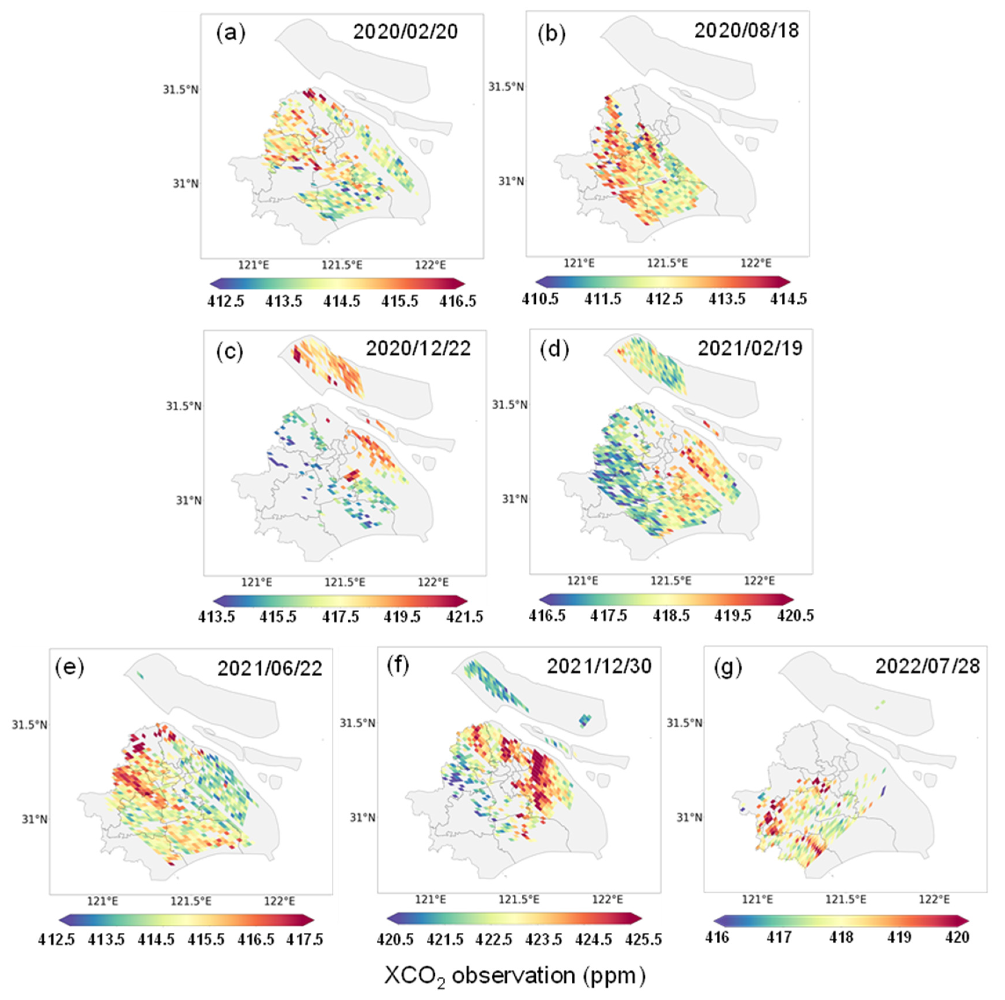
2.2. OCO-3 Snapshot XCO₂ Observations

OCO-3 operates below 52° latitude at an average altitude of approximately 400 km, completing one pass every 16 days and providing a spatial resolution of 1.6 km × 2.2 km. It is equipped with the same spectrometer as the OCO-2 satellite, achieving an observation precision of better than 1 ppm at 3 Hz [25]. Compared with OCO-2, the OCO-3 satellite introduced a new observation mode called ‘Snapshot Mode’. This mode leverages a pointing mirror assembly to independently scan a large area of approximately 80 × 80 km² during each satellite transit, capturing extensive XCO₂ data. This design effectively avoids the need for multiple repeated scans over small areas, as required in the Target mode of OCO-3, enabling a comprehensive coverage of CO₂ concentration in urban areas [28]. In this study, we utilize OCO-3 Level 2 Lite V10.4 Snapshot Mode XCO₂ data collected from January 2020 to December 2022 (https://disc.gsfc.nasa.gov/datasets/OCO3_L2_Lite_FP_10.4r/summary?keywords=oco3, last access: 11 October 2024). OCO-3 employs a quality filtering process to eliminate soundings that show larger than expected scatter differences in XCO2 compared to a “truth” metric [41]. Each sounding is assigned a quality flag (QF) of 0 (“good”) or 1 (“bad”). Additionally, OCO-3 considered footprint bias and parametric bias in XCO₂ [41,42,43,44]. To ensure data quality, only observations that had undergone bias correction and quality filtering (QF = 0) were selected for analysis [24]. In order to ensure an adequate footprint, we then screened the Snapshot Mode data over Shanghai from 2020 to 2022 with more than 300 effective footprints, identifying 7 days of available OCO-3 observations for our research (

Table 1. The transit time and number of footprints of the OCO-3 satellite Snapshot Mode data were adopted in this research. The simulation period corresponds to the transit time of the OCO-3 satellite Snapshot Mode over Shanghai. Since a single OCO-3 transit does not cover the entire city and some data are discarded during quality control, the number of footprints is not the same for each transit. We screened transit times with more than 300 effective footprints.

Date	Local Time	Number of Footprints
20 February 2020	14:05	541
18 August 2020	14:54	527
22 December 2020	13:03	343
19 February 2021	13:41	864
22 June 2021	12:57	761
30 December 2021	09:36	555
28 July 2022	14:17	337

).

2.3. Sentinel-5 TROPOMI NO₂ Observations

The combustion of fossil fuels not only releases CO₂ but also emits nitrogen oxide (NO_x = NO₂ + NO) into the atmosphere, which exists in the atmosphere mainly as nitrogen dioxide (NO₂). Due to the relatively short lifetime of NO₂ in urban areas compared to CO₂ (approximately 3 to 13 h) [45], and its concentration increment signal being significantly higher than the background level, NO₂ is often used to identify the source of CO₂ plume signals [31,46,47,48]. In this study, in addition to using XCO₂ data from the snapshot mode of the OCO-3 satellite as a reference for emission inventories, we also incorporated vertical column density (VCD) of NO₂ from the Sentinel-5 satellite Tropospheric Monitoring Instrument (TROPOMI) [49]. TROPOMI has a swath width of 2600 km, providing global coverage on a daily basis. The NO₂ VCD data used in this study were derived from the reprocessed (RPRO) Level 2 TROPOMI data product, which had undergone quality filtering. The spatial resolution is 3.5 km × 5.5 km, with a local overpass time of approximately 13:30. Following the method of Kiel et al. [26], we selected data within a ±3-h window around the OCO-3 overpass as valid observations.

2.4. WRF-CMAQ Model

The XCO₂ concentrations in Shanghai were simulated using the Weather Research & Forecasting Model-Community Multiscale Air Quality Modeling System (WRF-CMAQ) [50]. The WRF model (Version 4.0) [51] is an open-source atmospheric dynamics model developed by the National Center for Atmospheric Research (NCAR). It can simulate a variety of atmospheric processes and specific atmospheric physical parameters in the atmosphere, including winds, clouds, precipitation, temperature, relative humidity, etc. The CMAQ model (Version 5.0.2) [52] is a comprehensive model system for simulating atmospheric chemical processes and air quality, including pollutant species such as ozone (O₃) and particulate matter (PM). CMAQ enables the numerical simulations of atmospheric chemistry at different spatial and temporal scales and has been widely used in air quality research. Considering that CO₂ is a stable species and does not participate in any atmospheric chemistry in the atmosphere, atmospheric chemistry and aerosol processes were turned off in this study. A detailed parameterization scheme is provided in Table S1.

The driving data for the WRF model are the Final Operational Global Analysis data (FNL) with 1° × 1° spatial resolution and 6 h temporal resolution. These data are provided by the National Centers for Environmental Prediction (NCEP)/NCAR of the United States of America and cover the globe from historical to real time with high spatial and temporal resolution.

According to Brunner et al. [53], the turbulent structure of a plume can be captured by the WRF-CMAQ model at a resolution of 1 km or finer. Therefore, in this study, we configured WRF-CMAQ with a 4-layer nested domain, using grid resolutions of 27 km, 9 km, 3 km, and 1 km. The finest domain (domain 4) has a grid size of 297 × 294. In the vertical direction, 51 layers were set up in the WRF model, which were merged into 15 layers for CMAQ. Before the OCO-3 satellite overpass, a 72 h spin-up was run. Boundary conditions were derived from CO₂ concentrations in the Global Carbon Assimilation System version 2 (GCASv2) [54].

2.5. CO₂ Fluxes

2.5.1. Anthropogenic CO₂ Emission Inventory

In this study, we analyzed two widely used anthropogenic CO₂ emission inventories covering the entire Shanghai region: Multi-resolution Emission Inventory for China (MEIC) for 2020 [55] (Version 1.4, http://meicmodel.org.cn, last access: 23 December 2024), and ODIAC Fossil Fuel CO₂ Emissions Dataset for 2021 [56] (Version name: ODIAC2022, https://odiac.org/ index.html#/, last access: 23 December 2024). Moreover, we also assessed one local emission inventory (LOCAL) for 2020, compiled by the Shanghai Academy of Environmental Sciences [57].

The MEIC inventory integrates multiple data sources and employs both technology-based and dynamic process-based approaches to characterize emission sources. It provides monthly, sector-specific emissions data in five sectors, power, industry, residential, transportation, and agriculture, at a spatial resolution of 0.25° × 0.25° (Figure 2a and

Table 2. Annual emission in Shanghai and spatial resolution of different anthropogenic emission inventories.

Emission Inventory	Annual Emission (Mt a−1)	Spatial Resolution
MEIC	150	0.25° × 0.25°
ODIAC	322	1 km × 1 km
LOCAL	126	4 km × 4 km

). CO₂ emissions in China are calculated using methods outlined in the IPCC Guidelines (GL) for National Greenhouse Gas Inventories [58]. The activity rates were from the MEIC for China (MEIC-China) [59] and the Carbon Emission Accounts and Datasets (CEADs) [60]. The emission factors were derived from CEADs, based on the measurements of over 4000 coal mine samples in China. The sector factors were obtained from the Guidelines for Provincial Greenhouse Gas Inventory [61]. The activity rates of national total CO₂ emissions were downscaled to sub-country administrative divisions using the normalized proportional shares of sub-country activity rates to the country total. Additionally, the net caloric value of coal (per unit of fossil fuel burned) [62] was adjusted based on measured data from coal mine samples. The uncertainty of MEIC may originate from the differences in methodologies, data quality, emission factors, and definitions of multiple source data [55].

The ODIAC inventory is a high-resolution global emission data product of fossil fuel combustion, estimated from Carbon Dioxide Information Analysis Centre (CDIAC) emission dataset [63]. It includes point sources, nonpoint sources, cement production, gas flare, international aviation, and marine bunkers, at a spatial resolution of 1 km × 1 km (Figure 2c and Table 2). ODIAC uses satellite observations of nighttime lights as a proxy for industrial and residential areas to map the spatial distribution of global fossil fuel CO₂ emissions. Point sources in ODIAC are derived from the point source emissions database Carbon Monitoring and Action (CARMA, https://www.cgdev.org/topics/carbon-monitoring-action, last access: 23 December 2024). Emissions from gas flaring are distributed using a specialized nighttime light-based gas flare map. Emissions from international aviation are distributed using the AERO2k inventory [64], while international marine bunker emissions are distributed from EDGAR v4.1 [65]. Although the national emissions estimates have uncertainties ranging from 4.0% to 20.2%, the uncertainties in grid emissions data could reach up to 120%, according to Andres et al. [66,67]. These uncertainties arise from the use of proxies for spatial distribution rather than direct measurements. Moreover, disaggregation methods, temporal variability, global scaling, and spatial resolution may contribute to the uncertainties of ODIAC [56].

The LOCAL emission inventory, covering YRD at a spatial resolution of 4 km × 4 km [57] (Figure 2 and Table 2), estimates city-level high-resolution dynamic emissions of CO₂ by introducing dynamic temporal allocation coefficients based on real-time multi-source activity data and multiplying them by baseline emissions [68] for each subcategory. The baseline emission inventory was developed using a territorial-based approach defined by the World Resources Institute (WRI) and the World Business Council for Sustainable Development (WBCSD) [69]. LOCAL consists of five categories: power plants, heavy industry, light industry, mobile sources, and other sources. Other sources include residential sources, dust sources, oil storage and transportation, waste treatment and disposal, and agricultural sources. The real-time activity data it used include an Hourly Continuous Emission Monitoring System (CEMS) for energy-related industries; Vehicle Flow (VF), Ship Automatic Identification System (AIS), and Aircraft Land Takeoff (LTO) for mobile sources; and the Population Migration Index (PMI) to characterize daily emissions from residential sources [57]. Facilities in the power, heavy industry, and most light industry sectors were treated as point sources with precise geographic locations [70]. Uncertainty in the LOCAL emission inventory arises from several factors, including the limitations of the source of emissions data and the determination of dynamic temporal allocation coefficients, as CEMS data only monitor organized emissions [57].

It should be noted that to investigate the impact of different anthropogenic emission inventories on the simulations, we kept the emission inventory outside Shanghai consistent in all scenarios by using the highest-resolution publicly available emission inventory, ODIAC. While the choice of emission inventories may indeed influence study outcomes, this is the same for each of the simulation experiments and therefore does not affect the quantification of differences in the inventory simulations. In addition, Shanghai was mainly affected by southeasterly winds during these satellite transits, and east of Shanghai is the sea where anthropogenic emissions are very limited, so the uncertainty in emissions from neighboring regions outside of Shanghai has a weak impact on the simulations. Furthermore, for the comparison with OCO-3 XCO₂, the difference between simulated and observed XCO₂ concentration was used. Therefore, we believe that discrepancies in emission inventories for these peripheral areas have a limited impact on the result.

2.5.2. Ecosystem, Ocean, and Wildfire Carbon Fluxes

The XCO₂ concentration acquired by the OCO-3 satellite is the aggregate concentration field of multiple CO₂ sources, including not only anthropogenic emissions but also ecosystems, oceans, and wildfires emissions. Therefore, the contribution of these sources needs to be fully considered when modeling XCO₂ concentrations in WRF-CMAQ. The net carbon exchange between the land and atmosphere by an ecosystem or biological community is represented by Net Ecosystem Carbon Exchange (NEE), which was derived from the Boreal Ecosystem Productivity Simulator (BEPS) model [71,72] at a spatial resolution of 8 km × 8 km and a temporal resolution of 3 h. The BEPS model has been corrected with a large amount of driving force data at the site level. Harun et al. [73] and Kang et al. [74] have validated the BEPS results by the flux tower measurements. The ocean carbon flux represents the flux of CO₂ absorbed or released by the ocean from the atmosphere. These data were generated from GCASv2 [54], with a spatial resolution of 1° × 1° and a temporal resolution of 3 h. Finally, the wildfire carbon emission data were obtained from the Global Fire Emissions Database (GFED) v4.1s [75] with a spatial resolution of 0.25° × 0.25°. This dataset provides global estimates of burned area, monthly emissions, and contributions by fire type. To match the resolution of the WRF-CMAQ, we performed a spatial interpolation of all these fluxes.

2.6. The Calculation of Simulated XCO₂

We used two methods to calculate the simulated XCO₂. The first one, referred to as CMAQ weighted XCO₂ (or simply ‘weighted XCO₂’), is based on the formula from Connor et al. [76]. It combines the pressure weighting function and averaging kernel of each satellite transit to interpolate the simulated CO₂ concentration profiles onto the baroclinic layer of the satellite’s XCO₂ and then vertically integrates them according to the comparison of the magnitudes of the baroclinic pressures.

$$x_{c{o}_2}^m=x_{c{o}_2}^a+{\displaystyle \sum _{\mathrm{i}=1}^{\mathrm{j}}{h}_i{k}_i{(X_m-X_a)}_i}$$

(1)

$x_{C{O}_2}^m$ is the modeled weighted XCO₂, $x_{C{O}_2}^{\mathrm{a}}$ is the a priori XCO₂, j represents the total vertical layers in the OCO-3, i represents the number of vertical layers in the OCO-3, h_j is a pressure weighting function, k_j is the column-averaged kernel, X_m is a simulation of CO₂ that has been interpolated to the different pressure layers of OCO-3, and X_a is the a priori CO₂ concentration profile.

We also calculated the column-averaged CO₂ concentrations using CMAQ simulations based on O’Dell et al. [77] and named them CMAQ-averaged XCO₂ (averaged XCO₂). See Equations (2) and (3) for details:

$$X_{C{O}_2}={\displaystyle \frac{{\displaystyle \sum _{i=1}^{N-1}\overline{{(cu)}_i}}\mathrm{\Delta }{p}_i}{{\displaystyle \sum _{i=1}^{N-1}\overline{c_i}}\mathrm{\Delta }{p}_i}}$$

(2)

$$c\equiv {\displaystyle \frac{1-q}{g{M}_{air}}}$$

(3)

where $X_{c{o}_2}$ is the simulated mean XCO₂, i denotes the modeled vertical layer, u is the CMAQ-simulated CO₂ concentration, q is the specific humidity, $\overline{(cu){}_i}$ and $\overline{c_i}$ denote the mean values of the cu and c quantities over layer i, and ∆p_i is the barometric pressure difference between p_i and p_i+1.

3. Results

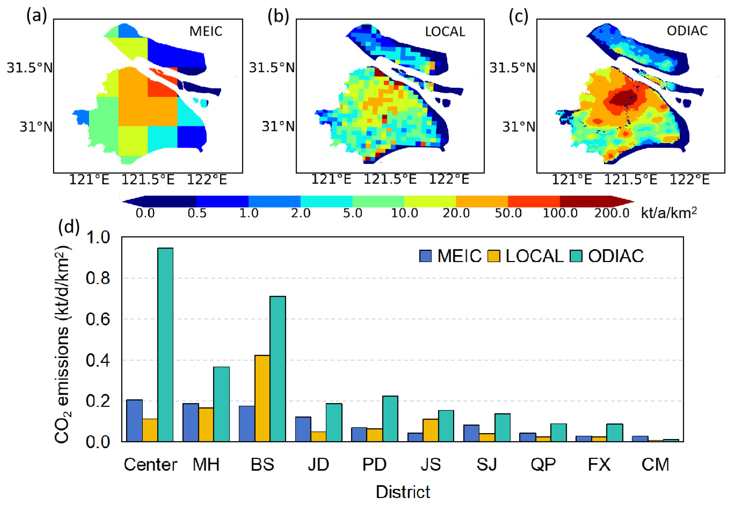
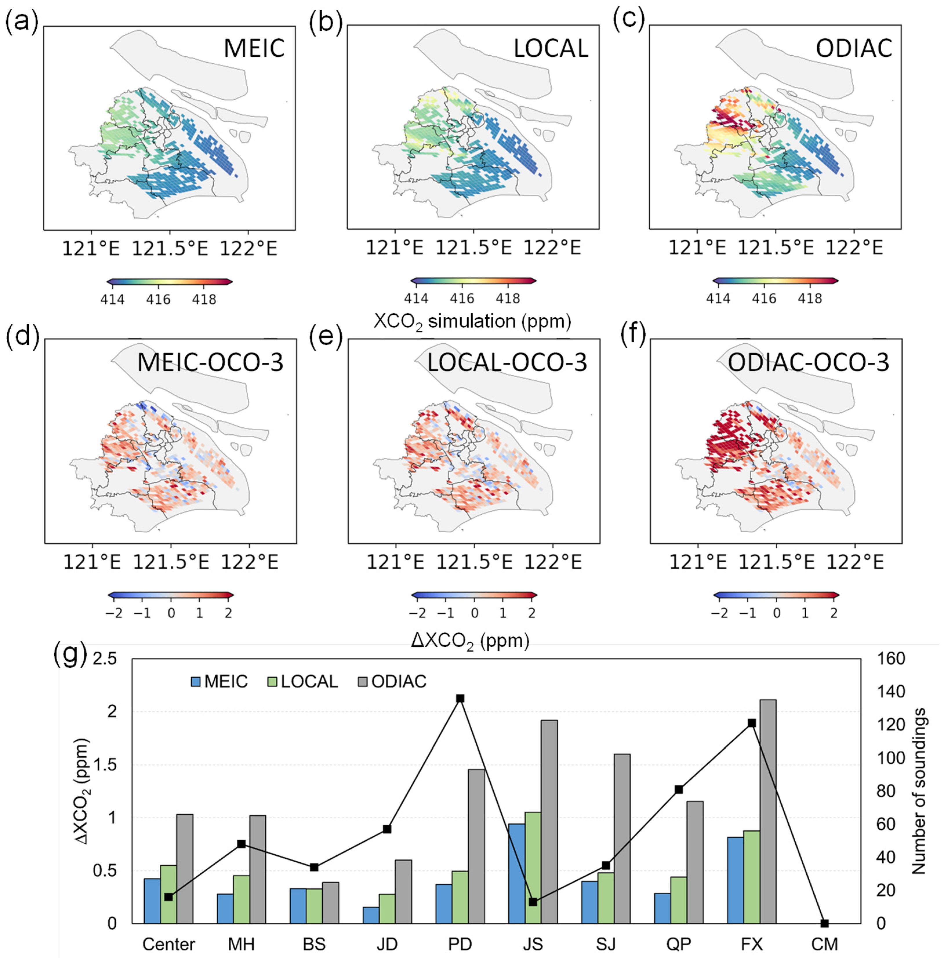
3.1. The Differences Between the CO₂ Anthropogenic Emission Inventories in Shanghai

The annual emissions and spatial resolutions of these emission inventories are shown in Table 2. The annual emissions for ODIAC, MEIC, and LOCAL are 322 Mt, 150 Mt, and 126 Mt, respectively, differing by roughly a factor of ~2.6 (Table 2). In terms of spatial resolution, MEIC is the coarsest, while ODIAC is the finest, with up to 20-fold difference. These discrepancies indicate that considerable uncertainty persists in anthropogenic CO₂ emission inventories.

We compared the spatial distributions of different anthropogenic emission inventories (Figure 2a–c). Although their spatial resolutions differ significantly, all inventories show an emission gradient from the Center area to the surrounding districts. For MEIC and ODIAC, emissions are highest in the Center area. However, for LOCAL, the region with the highest emission is BS. We also summed the emission rates in all districts (Figure 2d). Overall, the MEIC and LOCAL emission inventories yield lower emission rates than ODIAC in every district except CM. The area with the largest difference is the Center area, where ODIAC is 4.6 times higher than MEIC and 8.5 times higher than LOCAL. Comparing MEIC and LOCAL specifically, LOCAL exhibits higher emissions in BS and JS, whereas MEIC remains larger in the other districts. This discrepancy is largely attributable to LOCAL’s more detailed energy-related emission data.

In Shanghai, the three largest coal-fired power plants are located in BS, PD, and MH (Figure 1). As shown in Figure 2a, the coarse resolution of MEIC makes it difficult to reflect signals from coal-fired power plants, so the emissions in BS, PD, and MH are not prominent. The two largest power plants in BS and PD are not well represented in the Shanghai region (Figure 2b). By contrast, the LOCAL emission inventory incorporates data from local environmental monitoring authorities, so the latitude, longitude, and emissions of these power plants are comparatively accurate.

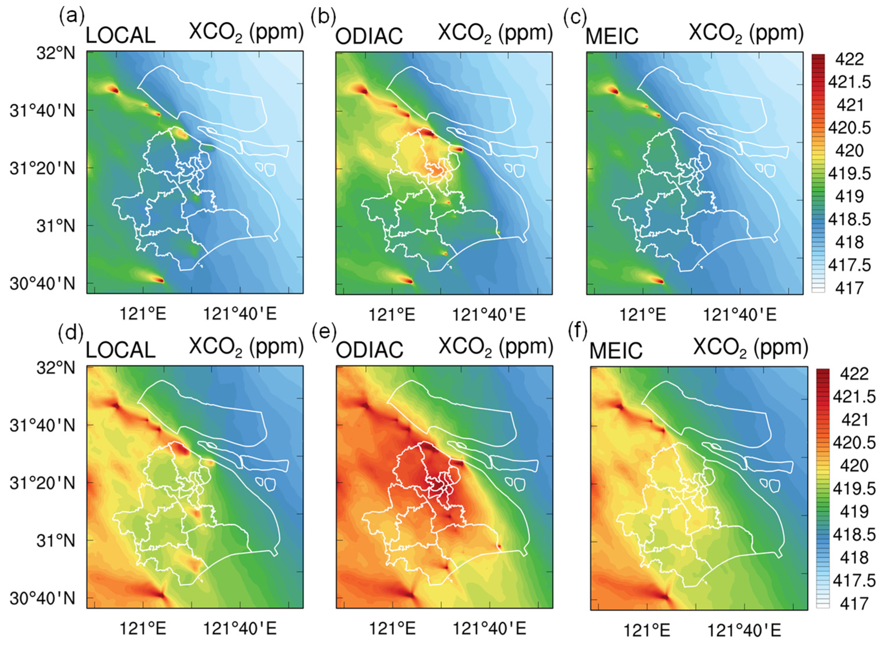
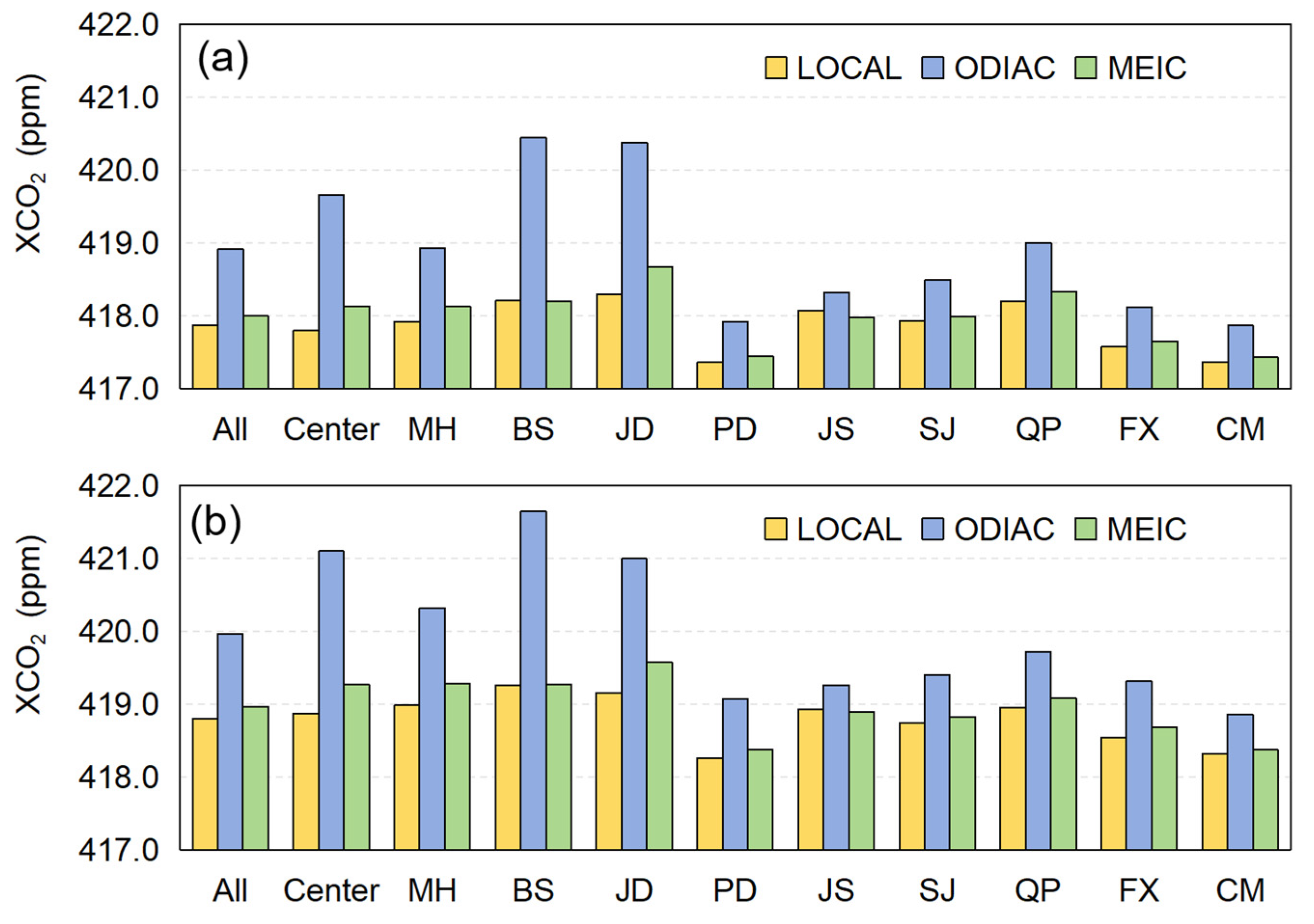
3.2. The Comparison of XCO₂ Simulations

We used three anthropogenic emission inventories to drive the CMAQ model and compute averaged XCO₂ values. The simulation period corresponds to the transit time of the OCO-3 satellite Snapshot Mode over Shanghai. Since a single OCO-3 transit does not cover the entire city and some data are discarded during quality control, we selected transit times with adequate data for analysis (Table 1). The initial field, boundary field, and external emission inventory for Shanghai remained consistent in all simulation experiments.

We analyzed the spatial distribution and regional mean simulated XCO₂ using the three emissions inventories in each transit (Figures S1 and S2) and then averaged all XCO₂ simulations in Figure 3a–c and Figure 4a. In the whole city, the ODIAC-based XCO₂ is notably higher than the LOCAL-based and MEIC-based XCO₂ by 1.04 ppm and 0.92 ppm, respectively (Figure 4a), consistent with differences among the emission inventories. Spatially, simulated XCO₂ in Shanghai is higher in the west and lower in the east, which may be attributed to sea–land effects in coastal areas. We averaged the 1000 hPa wind field for all transit times (Figure S3) and can see that the near-surface flow at these times was mainly from the southeast. This fully demonstrates that the oceanic air currents affect the spatial distribution of CO₂ in Shanghai, which may be the main reason why the simulated XCO₂ in Shanghai is higher in the west and lower in the east.

Considering that winter is the season with the weakest photosynthesis, lower ecosystem carbon fluxes accentuate the impact of anthropogenic emissions on XCO₂. The simulated regional average XCO₂ shows a positive correlation with the regional average emissions in all three emission inventories (Figure 5). The statistical significance of correlation coefficients was also assessed through a p-value analysis, yielding values of 0.07 (LOCAL inventory), 0.01 (ODIAC inventory), and 0.03 (MEIC inventory). The results indicate that the positive correlation between the LOCAL inventory and its modeled XCO₂ lacks statistical significance (p ≥ 0.05), whereas significant correlations were identified for the ODIAC and MEIC inventories (p < 0.05). Figure 3d–f show the average winter spatial distribution of XCO₂ simulated using different anthropogenic emission inventories. Clearly, the ODIAC-based simulations produce notably higher XCO₂ in the densely populated Center area, as well as BS, JD, and MH around the Center. In these regions, the average ODIAC-based XCO₂ in winter is 1.95 ppm and 1.67 ppm higher than the LOCAL-based and MEIC-based XCO₂, respectively (Figure 4b). In other regions, the ODIAC-based XCO₂ is only 0.54 ppm and 0.56 ppm higher than the LOCAL-based and MEIC-based XCO₂, respectively.

In the Center area, the ODIAC-based XCO₂ is 1.74 ppm higher than in other regions, whereas the LOCAL-based and MEIC-based values exceed other regions on average by only 0.44 ppm and 0.64 ppm, respectively. Although no large power plants are located in the central area, the population density is high, and ODIAC’s nighttime light data emphasize anthropogenic emissions in this region, leading to more pronounced differences from other inventories. Although a high-emitting power plant is located in the northernmost part of PD, the CO₂ it emits is transported downwind by the sea breeze, so PD is not considered an area of high ODIAC-based XCO₂. In contrast, although JD does not have major point sources, it lies near the Center area and downwind of two of the largest power plants in Shanghai, resulting in a prominent ODIAC-based XCO₂ region there.

LOCAL-based XCO₂ does not increase significantly in densely populated areas. XCO₂ in the Center area is comparable to the average values elsewhere. Relatively high XCO₂ values are observed primarily in areas with high-emission power plants, such as BS, MH, and JS, or in locations downwind of point sources, such as JD. LOCAL-based XCO₂ is lower than ODIAC-based XCO₂ in the same area with high-emission power plants. MEIC-based XCO₂ is comparable to LOCAL-based XCO₂, with just about 0.16 ppm higher. Due to its coarser resolution, MEIC is less effective at capturing plumes from point sources. Notably, JD—which is neither the most densely populated area nor home to any key sources—exhibits the highest simulated XCO₂, likely because it is downwind of major emission sites. These simulations provide a clear visual comparison of how different inventories influence XCO₂ in density-polluted areas, point source regions, and downwind zones.

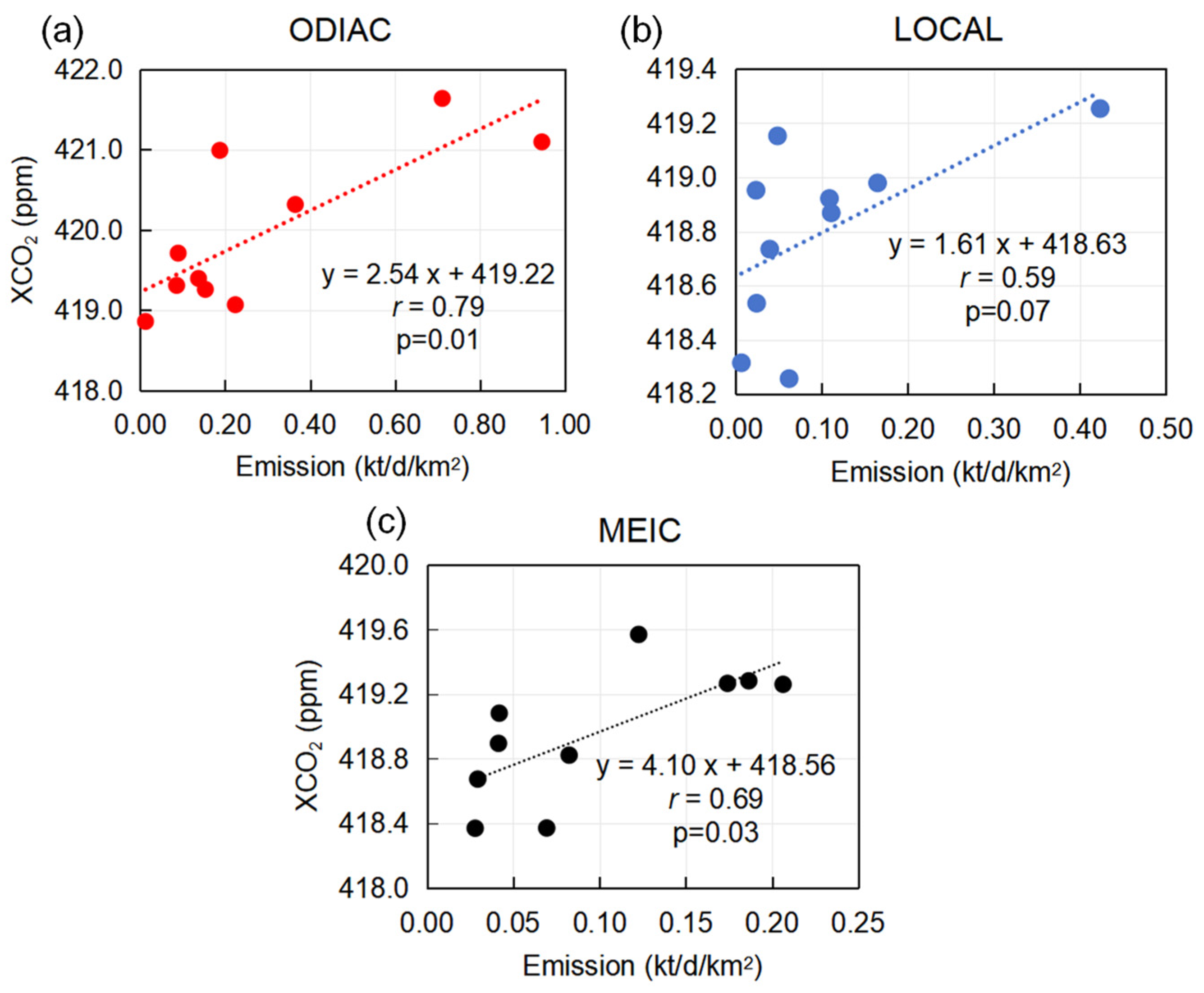
3.3. Comparison of Simulated XCO₂ with Satellite Observations

To evaluate the accuracy of the emission inventory, we introduced XCO₂ observations from the OCO-3 satellite Snapshot Mode and compared them with XCO₂ from the simulations. Figure 6 presents the OCO-3 satellite measurements, which cover multiple districts in Shanghai. These observations effectively characterize the intra-urban XCO₂ concentration gradient, especially the XCO₂ enhancements associated with point sources. This feature is consistently observed across all the transit times selected for this study.

Considering the satellite’s irregular coverage, we extracted the simulated XCO₂ for the same area (Figure 7a–c and Figure S4) and compared the differences between simulations and observations (∆XCO₂, simulations minus observations) for each satellite transit (Figure 7d–f and Figure S5). Overall, ∆XCO₂ was positive most of the time and across most areas, except in the northwestern part of the city, where negative ∆XCO₂ was observed. Citywide statistics indicate that the simulated XCO₂ concentration driven by all three emission inventories exceeds the observed XCO₂ by about 0.8 (±0.4) ppm on average for all transit.

For each transit, we calculated the regional ∆XCO₂ based on each of the three emission inventories (Figure 7g and Figure S6). Due to varying satellite coverage, certain areas may sometimes have too few footprints. Therefore, before averaging ∆XCO₂ for each district, we excluded regions with fewer than 10 footprints based on the number of soundings in every transit. The ecosystem carbon fluxes are smaller in winter, making it an ideal season for analyzing the spatial distribution of anthropogenic emission inventories. We then averaged the winter regional ∆XCO₂ for the different emission inventories and calculated the standard deviation (SD) and the coefficient of variation (CV) (

Table 3. The regional emissions (kt/d/km²) and ∆XCO₂ (ppm) in winter and their average (kt/d/km²; ppm), standard deviation (SD) (kt/d/km²; ppm), and coefficient of variation (CV) (%) over all regions. In addition, the regional population density (10,000 persons/km²) is also shown in the table.

District	Emission (kt/d/km2)			∆XCO2 (ppm)			Population Density (10,000 Persons/km2)
	MEIC	LOCAL	ODIAC	MEIC	LOCAL	ODIAC
Center	0.21	0.11	0.95	−1.26	−1.32	−0.10	2.19
MH	0.19	0.16	0.37	0.99	0.63	1.98	0.73
BS	0.17	0.42	0.71	−0.90	−0.93	−0.36	0.84
JD	0.12	0.05	0.19	−0.99	−0.89	−0.15	0.41
PD	0.07	0.06	0.22	0.35	0.16	1.39	0.48
JS	0.04	0.11	0.15	1.32	1.38	1.85	0.14
SJ	0.08	0.04	0.14	0.39	0.18	1.19	0.33
QP	0.04	0.02	0.09	−0.70	−0.72	0.28	0.19
FX	0.03	0.02	0.09	1.93	1.72	2.70	0.17
CM	0.03	0.01	0.01	−0.49	−0.61	−0.03	0.05
Average	0.10	0.10	0.29	0.06	−0.04	0.87
SD	0.07	0.12	0.30	1.09	1.03	1.08
CV	69.73	122.38	104.95	1824.80	−2580.86	124.54

). CV is a standardized measure of dispersion, expressed as a percentage. The value of the CV is equal to the standard deviation divided by the mean value. The results indicate that ODIAC-based XCO₂ is much higher than the observed values, whereas MEIC-based XCO₂ and LOCAL-based XCO₂ are closer to the observations, with ∆XCO₂ of 0.87 ppm, 0.06 ppm, and -0.04 ppm, respectively. Among the three inventories, LOCAL has the highest accuracy since the absolute value of its XCO₂ is the lowest. ODIAC substantially overestimates total CO₂ emissions in Shanghai, while MEIC and LOCAL inventories align more closely with actual total CO₂ emissions in Shanghai. The highest CV values in the emission data are observed in LOCAL. This indicates that although the average emissions and the average ∆XCO₂ simulation errors of LOCAL are relatively small, the regional variation in emission accuracy is significant.

We also found that ∆XCO₂ varies significantly across different regions, indicating that the accuracy of these emission inventories is not uniform across the study area. In the densely populated Centre area, ∆XCO₂ from ODIAC is only −0.1 ppm, but MEIC and LOCAL estimate XCO₂ well below the observed value. Other regions where ODIAC gives more accurate XCO₂ include QP, JD, and CM. The absence of large power plants in these areas suggests that ODIAC is relatively reliable in regions dominated by area emissions. Conversely, in PD, JS, SJ, and FX, which are relatively unpopulated even with large power plants, the ODIAC inventory has much higher ∆XCO₂ than LOCAL and MEIC. Considering that ODIAC captures power plant signals less strongly than the LOCAL inventory (Figure 2), this may imply that ODIAC may be overestimating area sources there. LOCAL underestimates emissions in the Centre, BS, JD, QP, and CM, which are all situated in northern and western Shanghai, downwind of the sea breeze. These underestimates for more densely populated districts (Center, BS, and JD) than for the relatively sparsely populated districts (QP and CM) imply that LOCAL may underestimate the emission intensities of area sources. Lastly, because of its coarser resolution, the MEIC inventory is unable to capture point source emissions accurately, resulting in a slight overestimation of overall CO₂ emissions in Shanghai.

To reveal the characteristics of different emission inventories, we compared the average NO₂ VCD in each administrative district with the average emissions in the same area by calculating the correlation coefficient between them for each transit. Due to excessive missing VCD data on 20 February 2020, we did not include it in our analysis. Table S2 presents the correlations for the remaining six transits. We found that the MEIC and LOCAL inventories showed a significant positive correlation during three transits, whereas ODIAC did not in any case. This further confirms our assessment that the errors in the ODIAC inventory are greater than those in the other two inventories.

Referring to the algorithm proposed by Zheng et al. [78] and Mao et al. [79], we use both the modeled and observed XCO₂ to calculate the emission inventory bias using the following equation:

$$\mathrm{\Delta }emissio{n}_i={\displaystyle \frac{XC{O}_{2\_simu\_i}-XC{O}_{2\_obs\_i}}{{\beta }_i}}$$

(4)

$${\beta }_i={\displaystyle \frac{1}{n}}{\displaystyle \sum _{j=1}^n\frac{{XCO}_{2\_simu\_i}-{XCO}_{2\_simu\_j}}{{emis}_i-{emis}_j}}$$

(5)

where ∆emission is the anthropogenic emission inventory bias; XCO_{2_simu} is the simulated XCO₂ value; XCO_{2_obs} is the observed XCO₂ value from the OCO-3 satellite; i is the anthropogenic emission inventory; j is one of the other anthropogenic emission inventories; and emis is the emission intensity, i.e., anthropogenic emissions per square kilometer per day. In this study, n is equal to 2. We accounted for the biases of the three emission inventories in each region (Figure 8). A positive (negative) ∆emission indicates that the inventory overestimates (underestimates) regional emissions, and the absolute value reflects the magnitude of this bias. Since emissions from CM are much lower than those from other regions, its emission bias is not considered here.

The three emission inventories underestimate emissions in Center, BS, and JD, while they overestimate emissions in FX, SJ, JS, PD, and MH. The ODIAC inventory is generally more accurate in densely populated areas (Center area, BS, and JD), where emission biases are only -0.06 to -0.01 kt/d/km². This may be related to the way the ODIAC inventory of area source emissions is allocated based on satellite light data. These three regions are densely populated areas with stronger lighting (Table 3), and the spatial allocation of regional emissions may be more accurate. However, it overestimates emissions in regions with relatively low population densities areas, whose emission biases are all around 0.22 kt/d/km². The LOCAL inventory underestimates emissions in the densely populated areas, but to a much greater extent than ODIAC. The largest underestimation occurs in the Center area and BS, which exhibit the highest population density citywide. This suggests that the LOCAL inventory likely fails to account for certain area emissions sources. Meanwhile, LOCAL is relatively accurate for MH and PD, where power plants are located. Although BS has a power plant, its high population density still leads LOCAL to underestimate emissions there. MEIC, although similar to LOCAL and significantly lower than ODIAC in terms of overall urban emissions, has the largest regional emission biases of the three emissions, with a maximum underestimation of 0.41 kt/d/km² and an overestimation of 0.73 kt/d/km².

4. Discussion

There are 36 central cities in China, and their total carbon emissions account for as much as 30.3% of the country’s total carbon emissions. Of these cities, 18 are in the top 30 CO₂ emitters in China, accounting for 22.2% of the country’s total carbon emissions [80]. Therefore, the key to achieving carbon neutrality in China lies in how central cities can take the lead in achieving a low-carbon transition. We need to have a clear and accurate picture of the current state of urban carbon emissions.

Emission inventories are an important source of information on the level of anthropogenic carbon emissions in cities. We focus on a city characterized by a high population density, diverse industries, and significant coverage by OCO-3 satellite observations: Shanghai, which is the city with the largest CO₂ emissions in China. We compared three CO₂ emission inventories: two global inventories (MEIC and ODIAC) and one provincial inventory (LOCAL). The primary goal is to evaluate both the spatial distribution and the accuracy of these emission inventories through comparisons of XCO₂ simulations generated by the WRF-CMAQ model with OCO-3 satellite Snapshot Mode observations.

These three anthropogenic CO₂ emission inventories differ substantially, varying by up to a factor of 2.6, with spatial resolutions differing by a factor of 20 or more. Oda et al. [81] compared ODIAC and the geoinformation technologies, spatio-temporal approaches, and full carbon account for improving the accuracy of GHG inventories (GESAPU) in Poland and agreed that although two emission inventories are in agreement in total and sectoral emissions, the emission spatial patterns showed large differences (10~100%). This reinforces the fact that even for carbon inventories with close emission totals, the spatial differences are still substantial.

The most pronounced discrepancy occurs in the most densely populated area region, where ODIAC’s emissions are 4.6 and 8.5 times higher than those of MEIC and LOCAL, respectively. Each inventory also identifies different regions as the highest emitters of CO₂. Both ODIAC and MEIC point to the central area of Shanghai, while LOCAL identifies the pronounced point source district, Baoshan, as the area with the greatest emissions. This is primarily related to the statistical methodology of the inventories.

The ODIAC inventory allocates area emissions by distributing the global fossil fuel CO₂ emissions dataset from CDIAC using satellite-observed nighttime light data. This approach results in an emission distribution closely tied to human nighttime activities, leading to the highest estimated emissions in the Center region. ODIAC’s point source data are derived from the CARMA point source emissions database, which has been shown to have considerable uncertainty, sometimes resulting in large point sources being misplaced [82]. The LOCAL inventory, compiled by the Shanghai Academy of Environmental Sciences, incorporates firsthand point source data, which are typically obtained directly from factories. As a result, the point sources in this inventory are relatively precise. The downscaling method of the MEIC inventory is also related to activity levels. Although its resolution is relatively coarse, it still estimates higher emissions in densely populated areas, leading to the highest emissions in the Center region. From the perspective of statistical methodology and emission distribution characteristics, the primary factors contributing to the spatial differences among these three emission inventories are likely twofold: the accuracy of point source emission estimates and the estimation of human activity levels.

It is worth noting that thermal power plants are the main source of anthropogenic CO₂, accounting for 40–50% of urban anthropogenic CO₂ emissions [62]. However, their spatial scales are often much smaller than the resolution of most emission inventories, making it challenging to capture their emissions accurately. The two largest CO₂ point sources in Shanghai—Shidongkou power plant in BS and Waigaoqiao power plant in PD—are clearly visible in LOCAL but appear less distinct in ODIAC and are missing in MEIC.

Based on the XCO₂ simulation results driven by different emission inventories, ODIAC-based XCO₂ is up to 1.04 ppm and 0.92 ppm higher than MEIC-based and LOCAL-based XCO₂, respectively, especially in densely populated areas (Central, BS, JD, and MH). LOCAL-based XCO₂ shows clear enhancements near power plants, while MEIC-based XCO₂ broadly resembles LOCAL’s except around power plants. By comparison with OCO-3 satellite Snapshot Mode XCO₂ observations, we found that LOCAL shows the highest accuracy, slightly underestimating emissions, while ODIAC overestimates them most. Regionally, ODIAC performs well in densely populated areas (with biases of only -0.06 to -0.01 kt/d/km²) but overestimates emissions (~0.22 kt/d/km²) in districts which are relatively unpopulated, even with large power plants. This finding is consistent with those of Chen et al. [14], who counted the differences between the inventories for 14 urban areas and the ODIAC inventory, found that the ODIAC inventory is overestimated by a relatively large margin in developing countries, and agreed that this may be related to the poor correlation between nighttime light intensity and human activity. However, we further discovered that ODIAC’s overestimation mainly occurs in sparsely populated areas. This is in very good agreement with the recent study in the Polang and the northeastern USA area [13,81]. This may be due to Shanghai’s highly developed road network, which maintains high nighttime light intensity in relatively unpopulated regions. In reality, excluding the road network, human activity-related light intensity in these areas may not be significant, and the emission-to-light ratio is much lower than in urban areas. As a result, emissions in less populated regions of Shanghai are overestimated. In contrast, LOCAL captures point source emissions relatively accurately, but it underestimates emissions in area sources. The underestimation in area is likely due to an underestimation of transport and residential emissions. In terms of the emission share of the LOCAL inventory, residential emissions account for ~5% and transport emissions account for ~18% [57]. This share is significantly lower than that of the latest Carbon Monitor Cities—China (CMCC), which shows the share of residential and transport shares are ~13.4% and ~23.0%, respectively [83].

For the uncertainty of the study results, we believe that it may come from the observational data, non-anthropogenic CO₂ emission source, atmospheric transport modeling, and the disparity of different types of emission sources. It is important to understand that although the reliability of Snapshot Mode observations has been well validated in many studies, XCO₂ observations are indirectly detected and therefore still not fully accurate. A comparison with ground-based TCCON (Total Carbon Column Observation Network) data shows single observation uncertainties of 0.5–1.5 ppm [23]. This leads to uncertainties in comparisons with inventories, especially in the case of insufficient spatial and temporal coverage of XCO₂ by OCO-3. The uncertainty of the ecosystem and ocean may also affect the results, e.g., although Harun et al. [73], and Kang et al. [74] validated the BEPS results though flux tower measurements, this does not mean that BEPS NEE modeling in the Shanghai region is absolutely accurate. Atmospheric transport modeling biases may also cause uncertainty in the results. WRF may have some overestimation of the wind field in Shanghai [84], which may lead to underestimation of the modeled concentrations and perhaps overestimation of the emissions. However, this overestimation of the wind field may be systematic for a city with a flat topography like Shanghai and may have limited impact on identifying differences in the spatial distribution of emissions. Moreover, the insignificant correlation between the LOCAL emission inventory and it driven XCO₂ concentration simulations also increase the uncertainty in the estimation of emission bias. The most possible reason for the insignificant LOCAL correlation is that point source emissions from the LOCAL emission inventory are significantly larger than those from area sources (Figure 2b). The cross-administrative transport of strong point source plumes results in some regions with weak emissions still having high concentrations. Future work may need to split the large point sources and estimate the contribution of point sources and area sources to XCO₂ concentrations separately.

5. Conclusions

Generally, ODIAC substantially overestimates total CO₂ emissions in Shanghai, while the MEIC and LOCAL inventories align more closely with actual total CO₂ emissions in Shanghai. However, the comparison of emission inventories reveals significant discrepancies in both the spatial distribution and accuracy of anthropogenic CO₂ emissions over Shanghai. LOCAL generally performs the best in terms of accuracy, slightly underestimating area emissions but capturing the power plant emissions more accurately. ODIAC, on the other hand, overestimates emissions, though it performs well in densely populated areas. MEIC, with its coarse spatial resolution, leads to the largest regional errors.

This study not only characterizes the spatial distribution of the most commonly used urban CO₂ anthropogenic emission inventories but also reveals their precision errors, which are critical assumptions in urban carbon inversion.

References

1. Seto, K.C.; Dhakal, S.; Bigio, A.; Blanco, H.; D’elgado, G.; Dewar, D.; Huang, L.; Inaba, A.; Kansal, A.; Lwasa, S.; et al. Human settlements, infrastructure, and spatial planning. In Climate Change 2014: Mitigation of Climate Change. Contribution of Working Group III to the Fifth Assessment Report of the Intergovernmental Panel on Climate Change; Cambridge University Press: Cambridge, UK, 2014. [Google Scholar] [CrossRef]
2. Stocker, T.; Qin, D.; Plattner, G.K.; Tignor, M.; Allen, S.; Boschung, J.; Nauels, A.; Xia, Y.; Bex, V.; Midgley, P.M. Climate Change 2013: The Physical Science Basis. Contribution of Working Group I to the Fifth Assessment Report of the Intergovernmental Panel on Climate Change; Cambridge University Press: Cambridge, UK; New York, NY, USA, 2013; pp. 1–30. [Google Scholar] [CrossRef]
3. Qi, C.; Wang, Q.; Ma, X.; Ye, L.; Yang, D.; Hong, J. Inventory, environmental impact, and economic burden of GHG emission at the city level: Case study of Jinan, China. J. Clean. Prod. 2018, 192, 236–243. [Google Scholar] [CrossRef]
4. Cai, B.; Cui, C.; Zhang, D.; Cao, L.; Wu, P.; Pang, L.; Zhang, J.; Dai, C. China city-level greenhouse gas emissions inventory in 2015 and uncertainty analysis. Appl. Energy 2019, 253, 113579. [Google Scholar] [CrossRef]
5. Cai, B.; Lu, J.; Wang, J.; Dong, H.; Liu, X.; Chen, Y.; Chen, Z.; Cong, J.; Cui, Z.; Dai, C.; et al. A benchmark city-level carbon dioxide emission inventory for China in 2005. Appl. Energy 2019, 233, 659–673. [Google Scholar] [CrossRef]
6. Shan, Y.; Liu, J.; Liu, Z.; Shao, S.; Guan, D. An emissions-socioeconomic inventory of Chinese cities. Sci. Data 2019, 6, 190027. [Google Scholar] [CrossRef] [PubMed]
7. Shan, Y.; Guan, D.; Liu, J.; Mi, Z.; Liu, Z.; Liu, J.; Schroeder, H.; Cai, B.; Chen, Y.; Shao, S.; et al. Methodology and applications of city level CO2 emission accounts in China. J. Clean. Prod. 2017, 161, 1215–1225. [Google Scholar] [CrossRef]
8. Patiño-Aroca, M.; Parra, A.; Borge, R. On-road vehicle emission inventory and its spatial and temporal distribution in the city of Guayaquil, Ecuador. Sci. Total. Environ. 2022, 848, 157664. [Google Scholar] [CrossRef]
9. Jing, Q.; Bai, H.; Luo, W.; Cai, B.; Xu, H. A top-bottom method for city-scale energy-related CO2 emissions estimation: A case study of 41 Chinese cities. J. Clean. Prod. 2018, 202, 444–455. [Google Scholar] [CrossRef]
10. Han, P.; Zeng, N.; Oda, T.; Zhang, W.; Lin, X.; Liu, D.; Cai, Q.; Ma, X.; Meng, W.; Wang, G.; et al. A city-level comparison of fossil-fuel and industry processes-induced CO2 emissions over the Beijing-Tianjin-Hebei region from eight emission inventories. Carbon Balance Manag. 2020, 15, 1–16. [Google Scholar] [CrossRef]
11. Xu, Y.; Liu, Z.; Xue, W.; Yan, G.; Shi, X.; Zhao, D.; Zhang, Y.; Lei, Y.; Wang, J. Identification of on-road vehicle CO2 emission pattern in China: A study based on a high-resolution emission inventory. Resour. Conserv. Recycl. 2021, 175, 105891. [Google Scholar] [CrossRef]
12. Zhang, Q.; Boersma, K.F.; Zhao, B.; Eskes, H.; Chen, C.; Zheng, H.; Zhang, X. Quantifying daily NOx and CO2 emissions from Wuhan using satellite observations from TROPOMI and OCO-2. Atmospheric Meas. Tech. 2023, 23, 551–563. [Google Scholar] [CrossRef]
13. Gately, C.K.; Hutyra, L.R. Large Uncertainties in Urban-Scale Carbon Emissions. J. Geophys. Res. Atmos. 2017, 122, 11–242. [Google Scholar] [CrossRef]
14. Chen, J.; Zhao, F.; Zeng, N.; Oda, T. Comparing a global high-resolution downscaled fossil fuel CO2 emission dataset to local inventory-based estimates over 14 global cities. Carbon Balance Manag. 2020, 15, 1–15. [Google Scholar] [CrossRef] [PubMed]
15. Ogle, S.M.; Davis, K.; Lauvaux, T.; Schuh, A.; Cooley, D.; West, T.O.; Heath, L.S.; Miles, N.L.; Richardson, S.; Breidt, F.J.; et al. An approach for verifying biogenic greenhouse gas emissions inventories with atmospheric CO2concentration data. Environ. Res. Lett. 2015, 10, 034012. [Google Scholar] [CrossRef]
16. Su, M.; Shi, Y.; Yang, Y.; Guo, W. Impacts of different biomass burning emission inventories: Simulations of atmospheric CO2 concentrations based on GEOS-Chem. Sci. Total. Environ. 2023, 876, 162825. [Google Scholar] [CrossRef]
17. Ciais, P.; Crisp, D.; van der Gon, H.D.; Engelen, R.; Janssens-Maenhout, G.; Heiman, M.; Rayner, P.; Scholze, M. Towards a European Operational Observing System to Monitor Fossil: CO2 Emissions: Final Report from the Expert Group; European Commission: Brussels, Belgium, 2015. [Google Scholar] [CrossRef]
18. Duren, R.M.; Miller, C.E. Measuring the carbon emissions of megacities. Nat. Clim. Chang. 2012, 2, 560–562. [Google Scholar] [CrossRef]
19. Kort, E.A.; Frankenberg, C.; Miller, C.E.; Oda, T. Space-based observations of megacity carbon dioxide. Geophys. Res. Lett. 2012, 39, L17806. [Google Scholar] [CrossRef]
20. Lauvaux, T.; Miles, N.L.; Deng, A.; Richardson, S.J.; Cambaliza, M.O.; Davis, K.J.; Gaudet, B.; Gurney, K.R.; Huang, J.; O’Keefe, D.; et al. High-resolution atmospheric inversion of urban CO2 emissions during the dormant season of the Indianapolis Flux Experiment (INFLUX). J. Geophys. Res. Atmos. 2016, 121, 5213–5236. [Google Scholar] [CrossRef] [PubMed]
21. Yadav, V.; Ghosh, S.; Mueller, K.; Karion, A.; Roest, G.; Gourdji, S.M.; Lopez-Coto, I.; Gurney, K.R.; Parazoo, N.; Verhulst, K.R.; et al. The Impact of COVID-19 on CO2 Emissions in the Los Angeles and Washington DC/Baltimore Metropolitan Areas. Geophys. Res. Lett. 2021, 48, e2021GL092744. [Google Scholar] [CrossRef]
22. Lian, J.; Lauvaux, T.; Utard, H.; Bréon, F.-M.; Broquet, G.; Ramonet, M.; Laurent, O.; Albarus, I.; Cucchi, K.; Ciais, P. Assessing the Effectiveness of an Urban CO2 Monitoring Network over the Paris Region through the COVID-19 Lockdown Natural Experiment. Environ. Sci. Technol. 2022, 56, 2153–2162. [Google Scholar] [CrossRef]
23. Eldering, A.; Taylor, T.E.; O’Dell, C.W.; Pavlick, R. The OCO-3 mission: Measurement objectives and expected performance based on 1 year of simulated data. Atmospheric Meas. Tech. 2019, 12, 2341–2370. [Google Scholar] [CrossRef]
24. Taylor, T.E.; Eldering, A.; Merrelli, A.; Kiel, M.; Somkuti, P.; Cheng, C.; Rosenberg, R.; Fisher, B.; Crisp, D.; Basilio, R.; et al. OCO-3 early mission operations and initial (vEarly) XCO2 and SIF retrievals. Remote. Sens. Environ. 2020, 251, 112032. [Google Scholar] [CrossRef]
25. Osterman, G.; O’Dell, C.; Eldering, A.; Fisher, B.; Crios, D.; Cheng, C.; Frankenberg, C.; Lambert, A.; Gunson, M.; Mandrake, L.; et al. Orbiting Carbon Observatory-2 & 3 Data Product User’s Guide, Operational Level 2 Data Versions 10 and Lite File Version 10 and VEarly. 2020. Available online: https://docserver.gesdisc.eosdis.nasa.gov/public/project/OCO/OCO2_OCO3_B10_DUG.pdf (accessed on 11 October 2024).
26. Kiel, M.; Eldering, A.; Roten, D.D.; Lin, J.C.; Feng, S.; Lei, R.; Lauvaux, T.; Oda, T.; Roehl, C.M.; Blavier, J.-F.; et al. Urban-focused satellite CO2 observations from the Orbiting Carbon Observatory-3: A first look at the Los Angeles megacity. Remote Sens. Environ. 2021, 258, 112314. [Google Scholar] [CrossRef]
27. Zhou, M.; Ni, Q.; Cai, Z.; Langerock, B.; Nan, W.; Yang, Y.; Che, K.; Yang, D.; Wang, T.; Liu, Y.; et al. CO2 in Beijing and Xianghe Observed by Ground-Based FTIR Column Measurements and Validation to OCO-2/3 Satellite Observations. Remote. Sens. 2022, 14, 3769. [Google Scholar] [CrossRef]
28. Bell, E.; O’Dell, C.W.; Taylor, T.E.; Merrelli, A.; Nelson, R.R.; Kiel, M.; Eldering, A.; Rosenberg, R.; Fisher, B. Exploring bias in the OCO-3 snapshot area mapping mode via geometry, surface, and aerosol effects. Atmospheric Meas. Tech. 2023, 16, 109–133. [Google Scholar] [CrossRef]
29. Zhao, H.; Gui, K.; Yao, W.; Shang, N.; Zhang, X.; Zhang, X.; Li, L.; Zheng, Y.; Wang, Z.; Ren, H.; et al. Seasonal and Diurnal Variations in XCO2 Characteristics in China as Observed by OCO-2/3 Satellites: Effects of Land Cover and Local Meteorology. J. Geophys. Res. Atmos. 2023, 128, e2023JD038841. [Google Scholar] [CrossRef]
30. Chen, J.; Hu, R.; Chen, L.; Liao, Z.; Che, L.; Li, T. Multi-sensor integrated mapping of global XCO2 from 2015 to 2021 with a local random forest model. ISPRS J. Photogram. Rem. Sens. 2024, 208, 107–120. [Google Scholar] [CrossRef]
31. Lei, R.; Feng, S.; Xu, Y.; Tran, S.; Ramonet, M.; Grutter, M.; Garcia, A.; Campos-Pineda, M.; Lauvaux, T. Reconciliation of asynchronous satellite-based NO2 and XCO2 enhancements with mesoscale modeling over two urban landscapes. Remote. Sens. Environ. 2022, 281, 113241. [Google Scholar] [CrossRef]
32. Wu, D.; Liu, J.; Wennberg, P.O.; Palmer, P.I.; Nelson, R.R.; Kiel, M.; Eldering, A. Towards sector-based attribution using intra-city variations in satellite-based emission ratios between CO2 and CO. Atmospheric Meas. Tech. 2022, 22, 14547–14570. [Google Scholar] [CrossRef]
33. Yang, E.G.; Kort, E.A.; Ott, L.E.; Oda, T.; Lin, J.C. Using Space-Based CO2 and NO2 Observations to Estimate Urban CO2 Emissions. J. Geophys. Res. Atmos. 2023, 128, e2022JD037736. [Google Scholar] [CrossRef]
34. Hakkarainen, J.; Ialongo, I.; Oda, T.; Szeląg, M.E.; O’dell, C.W.; Eldering, A.; Crisp, D. Building a bridge: Characterizing major anthropogenic point sources in the South African Highveld region using OCO-3 carbon dioxide snapshot area maps and Sentinel-5P/TROPOMI nitrogen dioxide columns. Environ. Res. Lett. 2023, 18, 035003. [Google Scholar] [CrossRef]
35. Guo, W.; Shi, Y.; Liu, Y.; Su, M. CO2 emissions retrieval from coal-fired power plants based on OCO-2/3 satellite observations and a Gaussian plume model. J. Clean. Prod. 2023, 397, 136525. [Google Scholar] [CrossRef]
36. Roten, D.; Lin, J.C.; Das, S.; Kort, E.A. Constraining Sector-Specific CO2 Fluxes Using Space-Based XCO2 Observations Over the Los Angeles Basin. Geophys. Res. Lett. 2023, 50, e2023GL104376. [Google Scholar] [CrossRef]
37. Roten, D.; Lin, J.C.; Kunik, L.; Mallia, D.; Wu, D.; Oda, T.; Kort, E.A. The Information Content of Dense Carbon Dioxide Measurements from Space: An Urban-Focused Inversion Approach with Synthetic Data from the OCO-3 Instrument. ESS Open Archive. 2024, 28, 2024. [Google Scholar] [CrossRef]
38. Song, M.; Guo, X.; Wu, K.; Wang, G. Driving effect analysis of energy-consumption carbon emissions in the Yangtze River Delta region. J. Clean. Prod. 2015, 103, 620–628. [Google Scholar] [CrossRef]
39. Tian, G.; Jiang, J.; Yang, Z.; Zhang, Y. The urban growth, size distribution and spatio-temporal dynamic pattern of the Yangtze River Delta megalopolitan region, China. Ecol. Model. 2011, 222, 865–878. [Google Scholar] [CrossRef]
40. Li, J.; Zhou, H.; Meng, J.; Yang, Q.; Chen, B.; Zhang, Y. Carbon emissions and their drivers for a typical urban economy from multiple perspectives: A case analysis for Beijing city. Appl. Energy 2018, 226, 1076–1086. [Google Scholar] [CrossRef]
41. O’Dell, C.W.; Eldering, A.; Wennberg, P.O.; Crisp, D.; Gunson, M.R.; Fisher, B.; Frankenberg, C.; Kiel, M.; Lindqvist, H.; Mandrake, L.; et al. Improved retrievals of carbon dioxide from Orbiting Carbon Observatory-2 with the version 8 ACOS algorithm. Atmos. Meas. Tech. 2018, 11, 6539–6576. [Google Scholar] [CrossRef]
42. Wunch, D.; Toon, G.C.; Blavier, J.-F.L.; Washenfelder, R.A.; Notholt, J.; Connor, B.J.; Griffith, D.W.T.; Sherlock, V.; Wennberg, P.O. The Total Carbon Column Observing Network. Philos. Trans. R. Soc. A Math. Phys. Eng. Sci. 2011, 369, 2087–2112. [Google Scholar] [CrossRef]
43. Wunch, D.; Wennberg, P.O.; Osterman, G.; Fisher, B.; Naylor, B.; Roehl, C.M.; O’Dell, C.; Mandrake, L.; Viatte, C.; Kiel, M.; et al. Comparisons of the Orbiting Carbon Observatory-2 (OCO-2) XCO2 measurements with TCCON. Atmos. Meas. Tech. 2017, 10, 2209–2238. [Google Scholar] [CrossRef]
44. Kiel, M.; O’Dell, C.W.; Fisher, B.; Eldering, A.; Nassar, R.; MacDonald, C.G.; Wennberg, P.O. How bias correction goes wrong: Measurement of XCO2 affected by erroneous surface pressure estimates. Atmospheric Meas. Tech. 2019, 12, 2241–2259. [Google Scholar] [CrossRef]
45. de Foy, B.; Lu, Z.; Streets, D.G.; Lamsal, L.N.; Duncan, B.N. Estimates of power plant NOx emissions and lifetimes from OMI NO2 satellite retrievals. Atmospheric Environ. 2015, 116, 1–11. [Google Scholar] [CrossRef]
46. Reuter, M.; Buchwitz, M.; Schneising, O.; Krautwurst, S.; O’Dell, C.W.; Richter, A.; Bovensmann, H.; Burrows, J.P. Towards monitoring localized CO2 emissions from space: Co-located regional CO2 and NO2 enhancements observed by the OCO-2 and S5P satellites. Atmospheric Meas. Tech. 2019, 19, 9371–9383. [Google Scholar] [CrossRef]
47. Dou, X.; Wang, Y.; Ciais, P.; Chevallier, F.; Davis, S.J.; Crippa, M.; Janssens-Maenhout, G.; Guizzardi, D.; Solazzo, E.; Yan, F.; et al. Near-real-time global gridded daily CO2 emissions. Innovation 2021, 3, 100182. [Google Scholar] [CrossRef] [PubMed]
48. Le Quéré, C.; Jackson, R.B.; Jones, M.W.; Smith, A.J.P.; Abernethy, S.; Andrew, R.M.; De-Gol, A.J.; Willis, D.R.; Shan, Y.; Canadell, J.G.; et al. Temporary reduction in daily global CO2 emissions during the COVID-19 forced confinement. Nat. Clim. Chang. 2020, 10, 647–653. [Google Scholar] [CrossRef]
49. van Geffen, J.; Boersma, K.F.; Eskes, H.; Sneep, M.; ter Linden, M.; Zara, M.; Veefkind, J.P. S5P TROPOMI NO2 slant column retrieval: Method, stability, uncertainties and comparisons with OMI. Atmospheric Meas. Tech. 2020, 13, 1315–1335. [Google Scholar] [CrossRef]
50. Wong, D.C.; Pleim, J.; Mathur, R.; Binkowski, F.; Otte, T.; Gilliam, R.; Pouliot, G.; Xiu, A.; Young, J.O.; Kang, D. WRF-CMAQ two-way coupled system with aerosol feedback: Software development and preliminary results. Geosci. Model Dev. 2012, 5, 299–312. [Google Scholar] [CrossRef]
51. Skamarock, W.C.; Klemp, J.B.; Dudhia, J.; Gill, D.O.; Zhiquan, L.; Berner, J.; Wang, W.; Powers, J.G.; Duda, M.G.; Barker, D.M.; et al. A Description of the Advanced Research WRF Model Version 4; National Center for Atmospheric Research: Boulder, CO, USA, 2019; Volume 145. [Google Scholar] [CrossRef]
52. Byun, D.; Ching, J. Science Algorithms of the EPA Models-3 Community Multiscale Air Quality (CMAQ) Modeling System; Environmental Protection Agency: Washington, DC, USA, 1999; EPA600/R-99/030. [Google Scholar]
53. Brunner, D.; Kuhlmann, G.; Henne, S.; Koene, E.; Kern, B.; Wolff, S.; Voigt, C.; Jöckel, P.; Kiemle, C.; Roiger, A.; et al. Evaluation of simulated CO2 power plant plumes from six high-resolution atmospheric transport models. Atmospheric Meas. Tech. 2023, 23, 2699–2728. [Google Scholar] [CrossRef]
54. Jiang, F.; Wang, H.; Chen, J.M.; Ju, W.; Tian, X.; Feng, S.; Li, G.; Chen, Z.; Zhang, S.; Lu, X.; et al. Regional CO2 fluxes from 2010 to 2015 inferred from GOSAT XCO2 retrievals using a new version of the Global Carbon Assimilation System. Atmospheric Meas. Tech. 2021, 21, 1963–1985. [Google Scholar] [CrossRef]
55. Xu, R.; Tong, D.; Xiao, Q.; Qin, X.; Chen, C.; Yan, L.; Cheng, J.; Cui, C.; Hu, H.; Liu, W.; et al. MEIC-global-CO2: A new global CO2 emission inventory with highly-resolved source category and sub-country information. Sci. China Earth Sci. 2023, 67, 450–465. [Google Scholar] [CrossRef]
56. Oda, T.; Maksyutov, S. ODIAC Fossil Fuel CO2 Emissions Dataset (Version Name: ODIAC2022); Center for Global Environmental Research, National Institute for Environmental Studies: Tsukuba, Japan, 2015. [Google Scholar] [CrossRef]
57. Huang, C.; An, J.; Wang, H.; Liu, Q.; Tian, J.; Wang, Q.; Hu, Q.; Yan, R.; Shen, Y.; Duan, Y.; et al. Highly Resolved Dynamic Emissions of Air Pollutants and Greenhouse Gas CO2 during COVID-19 Pandemic in East China. Environ. Sci. Technol. Lett. 2021, 8, 853–860. [Google Scholar] [CrossRef]
58. Intergovernmental Panel on Climate Change (IPCC). IPCC Guidelines for National Greenhouse Gas Inventories 2006; Institute for Global Environmental Strategies: Kanagawa, Japan, 2006. [Google Scholar]
59. Zheng, B.; Tong, D.; Li, M.; Liu, F.; Hong, C.; Geng, G.; Li, H.; Li, X.; Peng, L.; Qi, J.; et al. Trends in China’s anthropogenic emissions since 2010 as the consequence of clean air actions. Atmospheric Meas. Tech. 2018, 18, 14095–14111. [Google Scholar] [CrossRef]
60. Cui, C.; Li, S.; Zhao, W.; Liu, B.; Shan, Y.; Guan, D. Energy-related CO2 emission accounts and datasets for 40 emerging economies in 2010–2019. Earth Syst. Sci. Data 2023, 15, 1317–1328. [Google Scholar] [CrossRef]
61. Department of Climate Change of National Development and Reform Commission. 2011. Available online: http://www.cbcsd.org.cn/sjk/nengyuan/standard/home/20140113/download/shengjiwenshiqiti.pdf (accessed on 15 January 2025).
62. IEA. World Energy Outlook 2022; International Energy Agency: Paris, France, 2022. [Google Scholar]
63. Gilfillan, D.; Marland, G. CDIAC-FF: Global and national CO2 emissions from fossil fuel combustion and cement manufacture: 1751–2017. Earth Syst. Sci. Data 2021, 13, 1667–1680. [Google Scholar] [CrossRef]
64. Eyers, C.J.; Norman, P.; Middel, J.; Plohr, M.; Michot, S.; Atkinson, K.; Christou, R.A. AERO2k Global Aviation Emissions Inventories for 2002 and 2025. 2005. Available online: https://elib.dlr.de/1328/ (accessed on 15 January 2025).
65. JRC: EDGAR—Emissions Database for Global Atmospheric Research. Available online: http://edgar.jrc.ec.europa.eu/ (accessed on 15 January 2025).
66. Andres, R.J.; Boden, T.A.; Higdon, D. A new evaluation of the uncertainty associated with CDIAC estimates of fossil fuel carbon dioxide emission. Tellus B: Chem. Phys. Meteorol. 2014, 66, 23616. [Google Scholar] [CrossRef]
67. Andres, R.J.; Boden, T.A.; Higdon, D.M. Gridded uncertainty in fossil fuel carbon dioxide emission maps, a CDIAC example. Atmospheric Meas. Tech. 2016, 16, 14979–14995. [Google Scholar] [CrossRef]
68. An, J.; Huang, Y.; Huang, C.; Wang, X.; Yan, R.; Wang, Q.; Wang, H.; Jing, S.; Zhang, Y.; Liu, Y.; et al. Emission inventory of air pollutants and chemical speciation for specific anthropogenic sources based on local measurements in the Yangtze River Delta region, China. Atmospheric Meas. Tech. 2021, 21, 2003–2025. [Google Scholar] [CrossRef]
69. World Resources Institute (WRI) and the World Business Council for Sustainable Development (WBCSD). The Greenhouse Gas Protocol: A Corporate Accounting and Reporting Standard. Available online: https://www.ghgprotocol.org/corporate-standard (accessed on 20 January 2025).
70. Wang, Y.; Huang, C.; Hu, X.; Wei, C.; An, J.; Yan, R.; Liao, W.; Tian, J.; Wang, H.; Duan, Y.; et al. Quantifying the Impact of COVID-19 Pandemic on the Spatiotemporal Changes of CO2 Concentrations in the Yangtze River Delta, China. J. Geophys. Res. Atmos. 2023, 128, e2023JD038512. [Google Scholar] [CrossRef]
71. Chen, J.; Liu, J.; Cihlar, J.; Goulden, M. Daily canopy photosynthesis model through temporal and spatial scaling for remote sensing applications. Ecol. Model. 1999, 124, 99–119. [Google Scholar] [CrossRef]
72. Ju, W.; Chen, J.M.; Black, T.A.; Barr, A.G.; Liu, J.; Chen, B. Modelling multi-year coupled carbon and water fluxes in a boreal aspen forest. Agric. For. Meteorol. 2006, 140, 136–151. [Google Scholar] [CrossRef]
73. Harun, F.; Soosaar, K.; Krasnova, A.; Pisek, J. Suitability of the boreal ecosystem simulator (BEPS) model for estimating gross primary productivity in hemi-boreal upland pine forest. For. Stud. 2021, 75, 1–14. [Google Scholar] [CrossRef]
74. Kang, F.; Li, X.; Du, H.; Mao, F.; Zhou, G.; Xu, Y.; Huang, Z.; Ji, J.; Wang, J. Spatiotemporal Evolution of the Carbon Fluxes from Bamboo Forests and their Response to Climate Change Based on a BEPS Model in China. Remote. Sens. 2022, 14, 366. [Google Scholar] [CrossRef]
75. Randerson, J.T.; Chen, Y.; van der Werf, G.R.; Rogers, B.M.; Morton, D.C. Global burned area and biomass burning emissions from small fires. J. Geophys. Res. Biogeosciences 2012, 117, G04012. [Google Scholar] [CrossRef]
76. Connor, B.J.; Boesch, H.; Toon, G.; Sen, B.; Miller, C.; Crisp, D. Orbiting Carbon Observatory: Inverse method and prospective error analysis. J. Geophys. Res. Atmos. 2008, 113, D5305. [Google Scholar] [CrossRef]
77. O’Dell, C.W.; Connor, B.; Bösch, H.; O’Brien, D.; Frankenberg, C.; Castano, R.; Christi, M.; Eldering, D.; Fisher, B.; Gunson, M.; et al. The ACOS CO2 retrieval algorithm—Part 1: Description and validation against synthetic observations. Atmospheric Meas. Tech. 2012, 5, 99–121. [Google Scholar] [CrossRef]
78. Zheng, B.; Zhang, Q.; Geng, G.; Chen, C.; Shi, Q.; Cui, M.; Lei, Y.; He, K. Changes in China’s anthropogenic emissions and air quality during the COVID-19 pandemic in 2020. Earth Syst. Sci. Data 2021, 13, 2895–2907. [Google Scholar] [CrossRef]
79. Mao, Y.; Wang, H.; Jiang, F.; Feng, S.; Jia, M.; Ju, W. Anthropogenic NOx emissions of China, the US and Europe from 2019 to 2022 inferred from TROPOMI observations. Environ. Res. Lett. 2024, 19, 054024. [Google Scholar] [CrossRef]
80. Cloud River Urban Research Institute. Available online: https://cici-index.com/en/881/ (accessed on 23 January 2025).
81. Oda, T.; Bun, R.; Kinakh, V.; Topylko, P.; Halushchak, M.; Marland, G.; Lauvaux, T.; Jonas, M.; Maksyutov, S.; Nahorski, Z.; et al. Errors and uncertainties in a gridded carbon dioxide emissions inventory. Mitig. Adapt. Strat. Glob. Change 2019, 24, 1007–1050. [Google Scholar] [CrossRef]
82. Gurney, K.R.; Liang, J.; O’Keeffe, D.; Patarasuk, R.; Hutchins, M.; Huang, J.; Rao, P.; Song, Y. Comparison of Global Downscaled Versus Bottom-Up Fossil Fuel CO2 Emissions at the Urban Scale in Four U.S. Urban Areas. J. Geophys. Res. Atmos. 2019, 124, 2823–2840. [Google Scholar] [CrossRef]
83. Huo, D.; Liu, K.; Liu, J.; Huang, Y.; Sun, T.; Sun, Y.; Si, C.; Liu, J.; Huang, X.; Qiu, J.; et al. Near-real-time daily estimates of fossil fuel CO2 emissions from major high-emission cities in China. Sci. Data 2022, 9, 1–21. [Google Scholar] [CrossRef]
84. Li, Y.; Jiang, F.; Jia, M.; Feng, S.; Lai, Y.; Ding, J.; He, W.; Wang, H.; Wu, M.; Wang, J.; et al. Improved estimation of CO2 emissions from thermal power plants based on OCO-2 XCO2 retrieval using inline plume simulation. Sci. Total. Environ. 2023, 913, 169586. [Google Scholar] [CrossRef]
Figure 1. The population density and districts of Shanghai. The red dots are power plants with a capacity greater than 450 W, and the size of the dots represents the relative capacity of the power plants. The black-framed area is the Center.
Remotesensing 17 01087 g001
Figure 2. The spatial distribution (ac) and the regional average emissions (d) of three anthropogenic CO2 emission inventories in Shanghai.
Remotesensing 17 01087 g002
Figure 3. Spatial distribution of simulated XCO2 using the three emissions inventories for all transits (ac) and winter transits (df). The dates for all transits are shown in Table 1, and the dates for winter transits are 20 February 2020, 22 December 2020, 19 February 2021, 30 December 2021. The white solid lines are the boundaries of Shanghai’s administrative districts.
Remotesensing 17 01087 g003
Figure 4. Regional average of XCO2 simulations in all transits (a) and winter (b) for LOCAL, ODIAC, and MEIC.
Remotesensing 17 01087 g004
Figure 5. Scatter plots and linear fits of regional average XCO2 simulations and emissions for different emission inventories in winter: (a) ODIAC; (b) LOCAL; and (c) MEIC. r is the correlation coefficient, which is significant when p < 0.05.
Remotesensing 17 01087 g005
Figure 6. The XCO2 observed by OCO-3 Snapshot Mode in every transit: (a) 20 February 2020; (b) 18 August 2020; (c) 22 December 2020; (d) 19 February 2021; (e) 22 June 2021; (f) 30 December 2021; and (g) 28 July 2022.
Remotesensing 17 01087 g006
Figure 7. The simulations of XCO2 and ∆XCO2 (simulations minus observations) on February 20, 2020, for three emission inventories: (ac) the XCO2 simulations of WRF-CMAQ; (df) the spatial distribution of ∆XCO2; (g) the regional average of ∆XCO2 (bars) and the number of soundings (black dotted line).
Remotesensing 17 01087 g007
Figure 8. Emission biases of all emission inventories. Positive (negative) bias indicates overestimation (underestimation) of emission inventories.
Remotesensing 17 01087 g008