Integrating Genetic Algorithm and Geographically Weighted Approaches into Machine Learning Improves Soil pH Prediction in China

Abstract

Accurate soil pH prediction is critical for soil management and ecological environmental protection. Machine learning (ML) models have been widely applied in the field of soil pH prediction. However, when using these models, the spatial heterogeneity of the relationship between soil and environmental variables is often not fully considered, which limits the predictive capability of the models, especially in large-scale regions with complex soil landscapes. To address these challenges, this study collected soil pH data from 4335 soil surface points (0–20 cm) obtained from the China Soil System Survey, combined with a multi-source environmental covariate. This study integrates Geographic Weighted Regression (GWR) with three ML models (Random Forest, Cubist, and XGBoost) and designs and develops three geographically weighted machine learning models optimized by Genetic Algorithms to improve the prediction of soil pH values. Compared to GWR and traditional ML models, the R² of the geographic weighted random forest (GWRF), geographic weighted Cubist (GWCubist), and geographic weighted extreme gradient boosting (GWXGBoost) models increased by 1.98% to 14.29%, while the RMSE decreased by 1.81% to 11.98%. Among the three models, the GWRF model performed the best and effectively reduced uncertainty in soil pH mapping. Mean Annual Precipitation and the Normalized Difference Vegetation Index are two key environmental variables influencing the prediction of soil pH, and they have a significant negative impact on the spatial distribution of soil pH. These findings provide a scientific basis for effective soil health management and the implementation of large-scale soil modeling programs.

1. Introduction

Soil pH is a key indicator reflecting the soil quality, playing a crucial role in agricultural productivity, environmental health, and ecosystem functions [1,2]. As the largest developing country and the leading consumer of nitrogen fertilizers, China faces a particularly severe soil acidification problem [3]. According to statistics, approximately 22.7% of the total soil in China is acidic, and the area of saline–alkali land spans 9.9 × 10⁷ ha [4,5]. The imbalance in soil pH directly affects key ecological processes, such as nutrient availability, microbial activity, pollutant migration, and plant growth [1,6], severely threatening food security, ecological integrity, and environmental safety in the region. However, traditional laboratory testing methods are expensive and inefficient, making large-scale, precise monitoring challenging. Therefore, the development of accurate spatial prediction methods for soil pH has become essential in precision agriculture and land management, providing essential support for optimizing land resource allocation, supporting scientific decision-making, and promoting the sustainable development of land resources.

With the advancement of digital soil mapping (DSM) technology, machine learning (ML) models have been widely used for soil property prediction, including the soil pH [7,8,9,10]. Techniques such as random forest (RF), Cubist, and eXtreme gradient boosting (XGBoost) models were widely applied in DSM [11,12,13]. Compared to traditional methods, ML, with its strong nonlinear fitting capability and flexibility, effectively overcomes the limitations of both parametric and non-parametric statistical approaches. For example, Hengl et al. [14] and Chagas et al. [15] compared the performance of linear regression and RF models in DSM, showing that the RF model outperformed the linear regression model. Hengl et al. [14] successfully predicted the global distribution of soil pH using ML techniques. Liu et al. [16] used the quantile RF model to predict the spatial distribution of soil pH in China. Furthermore, ML methods have less stringent requirements for the sample size, enabling precise predictions with fewer samples [17]. Chen et al. [12] successfully predicted soil pH values in China by integrating RF and XGBoost models with sparse sample data. These studies highlight the significant advantages of applying ML in spatial soil pH modeling, particularly in environments with limited data or highly nonlinear characteristics.

DSM is based on soil landscape theory, which aims to predict soil properties by utilizing spatial distribution patterns of environmental variables. This theory posits that the formation and distribution of soil are influenced by climate, biology, topography, parent material, and other environmental factors. Therefore, the performance of soil pH prediction depends largely on the environmental variables used for prediction model comstruction [18]. Numerous studies have demonstrated that topographic and climatic factors significantly impact the spatial distribution of soil pH. Castrignanò et al. [19] increased the accuracy of soil pH prediction in alpine dolines using a digital elevation model (DEM). Zhang et al. [20] reported that the annual average precipitation and temperature are key variables for soil pH prediction at the regional scale. In recent years, with the rapid development of remote sensing technologies (e.g., satellite remote sensing, drone monitoring, and ground sensors), an increasing number of studies have employed remote sensing imagery for soil pH estimation, providing novel technological approaches for large-scale soil pH monitoring and assessment [21,22,23].

Although the application of ML models has faciliated significant progress in soil pH prediction methods and the acquisition of environmental variables, it continues to face challenges and limitations. Notably, in existing ML models, it is typically assumed that the relationship between soil and the environment is stationary, suggesting that the impact of environmental variables on soil properties remains constant across different geographical locations. However, this assumption is not valid in practice [24]. In fact, the relationships between soil and the environment in different areas are nonstationary and heterogeneous, with spatial correlation. Failure to recognize such relationships in the modeling process may limit the model prediction performance, leading to significant uncertainties in the prediction results. To address these limitations, the Geographically Weighted Regression (GWR) method was integrated into the ML model to effectively reveal spatially nonstationary relationships between variables [25,26]. The GWR model captures spatial nonstationarity through the weighing of neighboring observations and the fitting of local regression models for specific locations. This enables the model to effectively capture spatial variations and reflect the local effects of environmental factors on soil properties. This method provides a promising opportunity to further enhance the accuracy of soil pH prediction. Additionally, parameter selection for most models relies on expert judgment and lacks adaptability to varying regional and environmental conditions, which affects the prediction accuracy and applicability of the model.

Based on this, we hypothesize that a geographically weighted ML (GWML) model with hyperparameter optimization can effectively improve model performance and be applied to spatial prediction of soil pH. To validate this hypothesis, we selected China, a region characterized by complex soil landscape structures, as the study area. We used large-scale soil pH data collected from 2010 to 2018, along with various environmental covariates. We attempted to combine geographically weighted regression (GWR) with three ML models (RF, Cubist, and XGBoost) and designed and developed three GWML models optimized by Genetic Algorithms (GAs) to improve the prediction of soil pH. The objectives of this study were (i) to compare the performance and uncertainty of three GA-optimized GWML models, (ii) to identify the most accurate model for predicting soil pH in China, and (iii) to determine the key factors influencing the spatial distribution of soil pH.

2. Materials and Methods

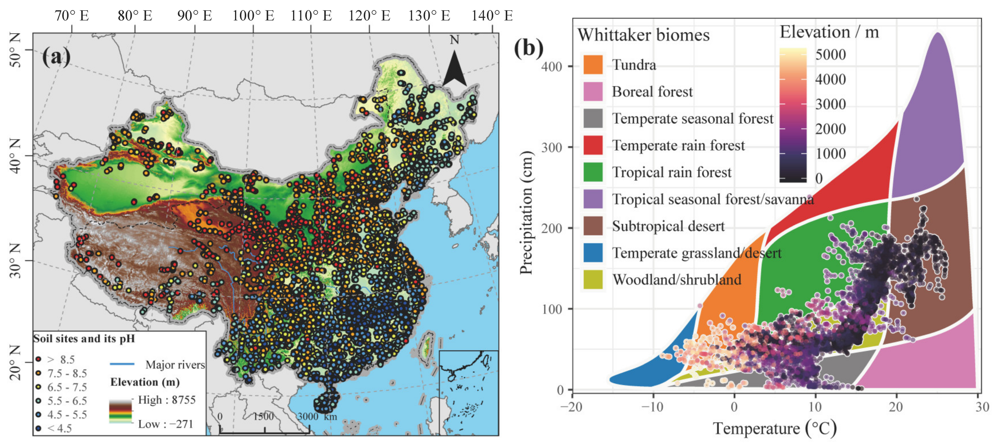
2.1. Soil Data

The 4335 soil profiles used in this study were sourced from the National Soil Series Survey published in the Soil Series of China (2009–2019), comprising 30 volumes [27]. These representative soil profiles cover various soil types across China. The geographic coordinates of all survey points were precisely recorded using a GPS receiver, and sampling was conducted according to different soil horizons. The pH values were then measured in the laboratory. All data were scanned, processed, validated, and subjected to three independent checks by different individuals to ensure consistency with the original dataset. To ensure comparability of soil properties across different profiles and mitigate the impact of variations between soil layers, we employed a spline tool (https://www.asris.csiro.au/methods.html accessed on 16 March 2024). For each pH profile, an automatic adaptive fitting procedure was applied with a threshold of 1.225 [16]. Moreover, mean soil pH values for the 0–20 cm layer of each profile was derived from the fitted curves (Figure 1).

2.2. Environmental Covariates

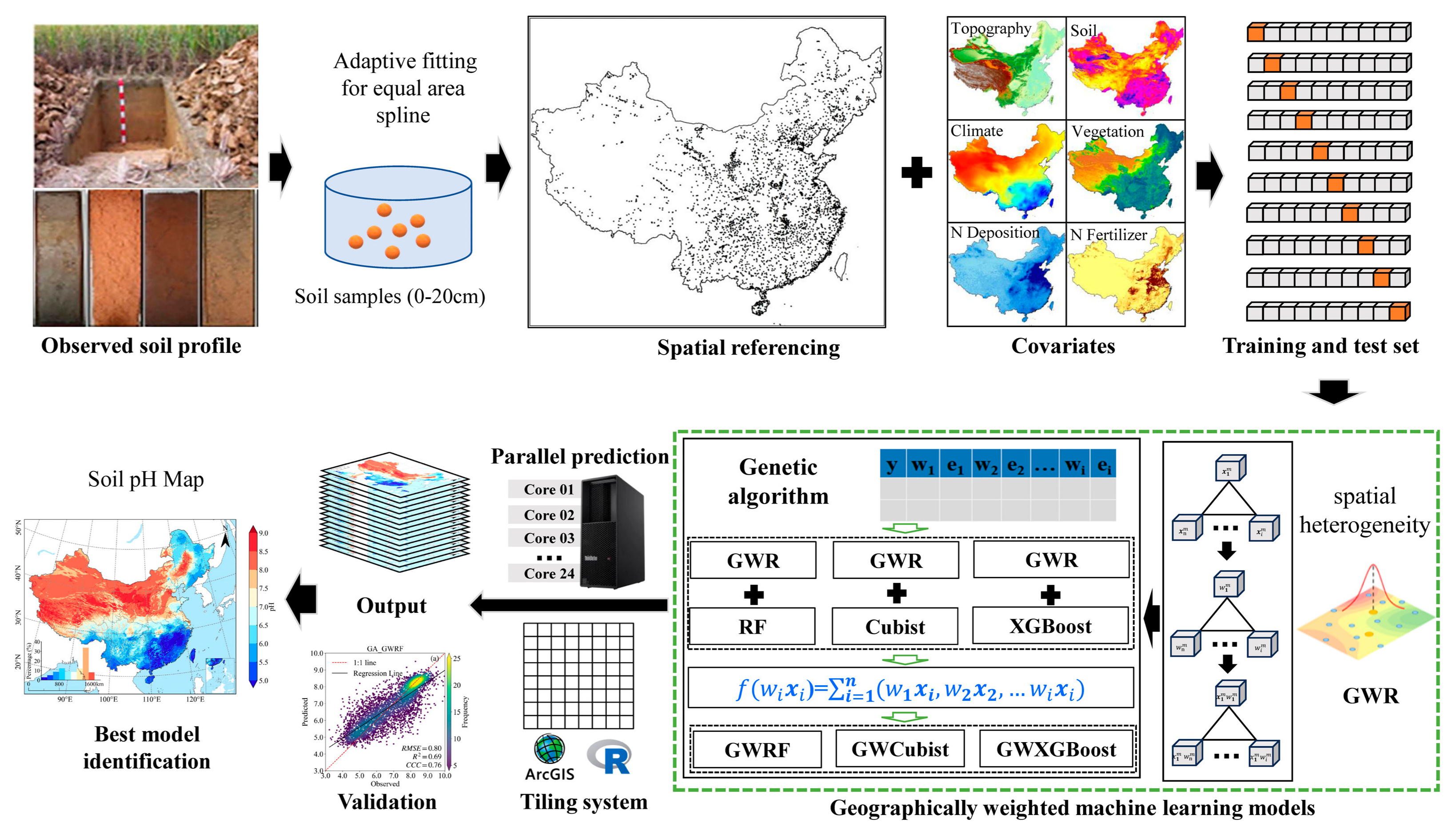
The spatial variation in soil pH is influenced by the interactions among terrain, climate, soil, vegetation, and human activities. Accordingly, these factors and process-related environmental covariates were considered in pH modeling. Data for a total of 19 environmental covariates were collected, and the variables were categorized into six groups, including soil properties, terrain characteristics, climate change, vegetation growth, and N input changes (

Table 1. Environmental covariates used for pH estimation.

Category	Covariates	Abbreviation	Resolution
Topography	Elevation	Ele	30 m
	Slope gradient	SG
	Multiresolution of ridge top flatness index	MRRTF
	Multiresolution Valley Bottom Flatness Index	MRVBF
	Terrain surface texture	TST
	Terrain Ruggedness Index	TRI
	Terrain surface convexity	TSC
	Channel Distance Base Level	CNBL
	Valley depth	VD
Soil	Sand content	Sand
	Silt content	Silt	250 m
	Clay content	Clay
Climate	Mean Annual Temperature	MAT	1 km
	Mean Annual Precipitation	MAP
Vegetation	Mean Normalized Difference Vegetation Index	NDVImean	250 m
	Net Primary Productivity	NPP	1 km
N input	Inorganic nitrogen dry deposition	INDD	10 km
	Inorganic nitrogen wet deposition	INWD	1 km
	Fertilizer (nitrogen)	Nfer	5 km

). Terrain information was derived from a 30 m digital elevation model (DEM) of the Shuttle Radar Topographic Mission (http://srtm.csi.cgiar.org/srtmdata/ accessed on 10 March 2024) obtained by using the System for Automated Geoscientific Analyses (SAGA) in Geographic Information System (GIS) software (version: 9.7.0). Soil texture data were obtained from the SoilGrids250m product (https://www.isric.org/ accessed on 12 March 2024), including sand, silt, and clay content. Climate data were acquired from the National Earth System Science Data Center (http://www.geodata.cn accessed on 12 March 2024). The mean normalized difference vegetation index (NDVI_mean) and the net primary productivity during the sampling period were extracted from Google Earth Engine. Wet nitrogen deposition data were collected from Chinese monitoring stations in 1996, and the dataset was interpolated and rasterized by kriging [28]. Dry nitrogen deposition data (2006–2015) were inferred from ground and space measurements via a remote sensing model and nonlinear regression methods involving convolutional neural networks [29,30]. National fertilizer inputs were provided by the Food and Agriculture Organization (FAO) (https://www.fao.org/faostat accessed on 17 October 2024) and the National Bureau of Statistics of China (Chinese Statistical Yearbook, also available from https://data.stats.gov.cn accessed on 17 October 2024). Considering the temporal inconsistency of spatial data, this study replaced all variable environmental factors with the multiyear averages over the sampling period to mitigate the potential impact of temporal changes on the results. Finally, all covariates were resampled to 1 km raster cells through the nearest neighbor and bilinear interpolation methods.

2.3. Methods

The relationships between the soil pH and environmental factors in large-scale complex regions are diverse and encompass both linear and nonlinear relationships. Moreover, they exhibit spatial heterogeneity. On this basis, we integrated GA and GWR methods into three ML models for predicting soil pH in China. The specific process is shown in Figure 2. First, we combined the 19 environmental covariates with the soil pH and calculated the spatial weights using the GWR method. The environmental covariates and their spatial weights were subsequently employed as input variables for the different GWML models. The GWML models were trained and tested by the 10-fold cross-validation method. Finally, the average of 10 sets of predictions of each GWML model was adopted as the final output, and the performance of the different GWML models was evaluated by the 10-fold cross-validation method.

2.3.1. Parameter Optimization

The Genetic Algorithm (GA) is an optimization algorithm based on natural selection and genetic mechanisms. The basic principle is to obtain the optimal solution via the continuous evolution of individuals (solutions) within the population, which is modeled on the basis of the evolutionary law of the selection and survival of the fittest in the biological world [31]. An initial set of solutions (referred to as the population) is established, and each solution (individual) consists of a set of parameters (genes). The GA aims to gradually improve upon the quality of the previous solution through selection, crossover, and mutation operations. In each generation, the strengths and weaknesses of the individuals are evaluated on the basis of a fitness function, and the best-performing individuals are selected as parents. New individuals (offspring) are generated through crossover operations, and mutations are introduced to increase diversity. After several iterative generations, the fitness of individuals within the population gradually increases to yield the global optimal solution. The GA is particularly suitable for solving complex, nonlinear, and multipeak optimization problems with notable robustness and global search capability.

2.3.2. Geographically Weighted Random Forest

The geographically weighted random forest (GWRF) model is an extension of the RF model tailored for geographic applications. A spatial weight matrix is generated by applying the principle of the GWR model to a nonlinear RF model. The results are then integrated into the theoretical framework of the RF model, and multiple decision trees are constructed via the random resampling bootstrap and random node splitting techniques to perform local regression with the spatial weight matrix. This approach can overcome the shortcomings of the traditional RF model in terms of spatial smoothness, effectively avoid covariance problems, and support the use of high-dimensional features. In addition, the improved model is less affected by noise and outliers, with a high learning speed and satisfactory model stability. In the model, three crucial parameters are important: the number of variables used to train each tree (mtry), the minimum number of terminal nodes (nodesize), and the number of trees to be generated (ntree).

2.3.3. Geographically Weighted Cubist Model

The geographically weighted Cubist model (GWCubist) model is an extension of the Cubist model designed for geographic applications. It incorporates the spatial weight matrix information from the GWR method into the theoretical framework of the Cubist model. A tree structure is created by combining soil observations and spatial weights, and then the regression tree is reduced to a set of comprehensible rules, which are obtained by if and else statements, of which each rule exhibits an associated multivariate linear model [32]. Unlike the classification and regression tree (CART) model, the Cubist model generates predictions via linear regression models rather than relying on discrete values [33], which can effectively capture the linear relationships and local spatial correlations between soil and environmental variables and improve prediction accuracy. The Cubist model includes two hyperparameters (the number of committees and the number of neighbors), which are used to increase its predictive performance.

2.3.4. Geographically Weighted eXtreme Gradient Boosting

The geographically weighted eXtreme gradient boosting (GWXGBoost) model is an extension of the XGBoost model in the field of geography. The GWR concept is applied to the XGBoost model, and a generative spatial weight matrix is incorporated into the theoretical framework of the XGBoost model. The idea is to integrate weak ML relationships to create a strong machine learner. The basic learner of the algorithm is the CART model, with soil observation data and spatial weights employed as inputs. Then, the initial CART model is generated, and the CART model that best improves the model is continuously adjusted with a greedy algorithm, which effectively improves the model accuracy [34]. Eight model parameters are important in this model: the number of iterations in model training (nrounds), the proportion of features used for training when building each tree (colsample_bytree), the sum of the minimum leaf node sample weights (min_child_weight), the learning rate (eta), the minimum loss needed for further leaf node splitting, the function descent value (gamma), the proportion of training data samples used to train each tree (subsample) and the maximum depth of trees (max_depth).

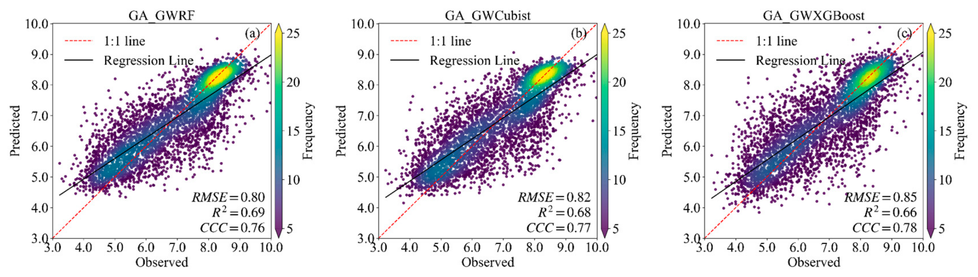
2.4. Evaluation of Model Performance

Based on 4335 soil surface pH data points, the 10-fold cross-validation method was used to evaluate the model performance. Specifically, the soil data were randomly divided into ten subsets. In each iteration, nine subsets were used for training, and the remaining subset was used for testing. This process was repeated ten times, with a different subset serving as the validation set in each iteration. Finally, the overall evaluation of the model was obtained by calculating the average of the ten validation results. To ensure unbiased model sampling, we assessed the spatial representativeness of the training samples during model construction by semivariance function analysis. The root mean square error (RMSE), coefficient of determination (R²), and concordance correlation coefficient (CCC) were employed to evaluate the different models. These metrics were calculated as follows:

$$RMSE=\sqrt{{\displaystyle \frac{1}{n}}{\sum }_{i=1}^n({e_i-o_i)}^2}$$

(1)

$$R^2=1-{\displaystyle \frac{{\sum }_{i=1}^n({e_i{-o}_i)}^2}{{\sum }_{i=1}^n({o_i-\overline{o})}^2}}$$

(2)

$$CCC={\displaystyle \frac{2r{\sigma }_e{\sigma }_o}{{\sigma }_e^2+{\sigma }_o^2+{(\overline{e}-\overline{o})}^2}}$$

(3)

where $e_i$ and $o_i$ are the predicted and observed values of soil pH values at sample point i; $n$ is the total number of sample points; $\overline{e}$ and $\overline{o}$ are the averages of the predicted and observed values, and ${\sigma }_e$ and ${\sigma }_o$ are the standard deviations of the predicted and observed soil pH values, respectively.

We derived prediction intervals through the 90% confidence interval (CI) calculated as μ ± 1.645σ for 10 GWML simulations [35]. The uncertainties in the estimates of the different models were quantified according to the specifications of GlobalSoilMap [36]. In addition, we compared our soil pH predictions with existing soil pH maps. These soil pH maps were sourced the National Soil Information Grids of China (NSGC) [16], SoilGrids250m [14], soil property distribution in China (SPDC) [37], and Harmonized World Soil Database 2.0 (HWSD2.0) [38]. To ensure comparability of the soil pH maps with existing soil maps, we used the spline tool, and equal-area quadratic splines were employed to fit the pH profile at each geographical location. From the fitted curve, we derived the mean soil pH over the 0–20 cm depth interval at each location. These values were used to create a standardized soil pH map. The improvement in the map based on our predictions relative to a previous soil map was calculated on the basis of the R² and RMSE as follows:

$${RI}_{R^2}={\displaystyle \frac{R_{our}^2-R_{ref}^2}{R_{ref}^2}}$$

(4)

$${RI}_{RMSE}={\displaystyle \frac{{RMSE}_{our}-{RMSE}_{ref}}{{RMSE}_{ref}}}$$

(5)

where ${RI}_{R^2}$ and ${RI}_{RMSE}$ are the relative improvements in the map based on our predictions for the R² and RMSE values, respectively. $R_{our}^2$ and ${RMSE}_{our}$ are the accuracy measurements for the map based on our predictions, and $R_{ref}^2$ and ${RMSE}_{ref}$ are the accuracy metrics for the reference map.

2.5. Data Processing

We created a 1 km × 1 km grid for the study area in ArcGIS 10.8. Data for the 19 variables involved in model training were extracted via the extract function in the “raster” package (version: 3.6-31). The GWML models were implemented in the open-source R environment. Prediction models for soil pH were built with the “GWmodel” (version: 2.4-1), “randomForest (version: 4.7-1.2)”, “Cubist” (version: 0.4.4), and “xgboost” packages (version: 1.7.8.1). We used the “GA” package (version: 3.2.4) in R to optimize these two parameters and then used the optimal parameter values as the final inputs (Table S1). Owing to the large size of the study area, prediction calculations were performed for 9,862,044 image elements, posing a substantial challenge given the computing power of ordinary computers. To accelerate the computations, we divided the data into 1000 parts by using a machine with 24 CPU cores to parallelize the computation. We then combined the 1000 parts of the data as the final output of the model. We visualized the data using ArcGIS 10.8, the “ggplot2” package for R software (version: 4.3.3), and the cartopy library in Python (version: 3.9.7).

3. Results and Analysis

3.1. Statistical Analysis of the Soil pH Data

The mean soil pH at the surface in China was 6.83 ± 1.45 (Figure 3a). Both acidified and alkaline soils accounted for 42% of the total number of samples, whereas neutral soils accounted for only 16% of the total samples. The initial distribution of the soil pH data was bimodal and did not pass the Shapiro–Wilk normality test, indicating that the data did not conform to a normal distribution (Figure 3a). To eliminate this bias and bring the data closer to a normal distribution, we applied the quantile transformer. After the quantile transformer, the distribution of the soil pH data conformed with a normal distribution (Figure 3b). The transformed data were subsequently used for subsequent statistical analysis to ensure the validity and robustness of the results.

3.2. Model Performance Comparison

The 10-fold cross-validation results indicated that the performance of the different geographically weighted models varied (Figure 4a–c). The RMSE values of the GA_GWRF, GA_GWCubist, and GA_GWXGBoost models were 0.80, 0.82, and 0.85, respectively, indicating that the GA_GWRF model has the lowest prediction error. In terms of goodness of fit, the R² values for GA_GWRF, GA_GWCubist, and GA_GWXGBoost were 0.69, 0.68, and 0.66, with GA_GWRF exhibiting the best fit. Regarding consistency, the CCC values for the three models were 0.76, 0.77, and 0.78, with GA_GWXGBoost showing the highest consistency. Overall, the performance of the different GWML models can be ranked as GA_GWRF > GA_GWCubist > GA_GWXGBoost.

Compared with traditional ML models (Figure S1), the performance of GA-optimized GWML models was higher, and the degree of enhancement varied depending on the model type (

Table 2. Degree of improvement in the GWML models based on GA-optimized models over traditional ML and GWR models.

Models	ML		GWR
	RIRMSE	RIR²	RIRMSE	RIR²
GWRF	2.14	1.98	11.55	14.29
GWCubist	2.66	2.78	9.43	11.82
GWXGBoost	1.81	2.04	6.38	8.61

). Specifically, compared with those of the RF model, the RMSE of the GWRF model decreased (2.14%), whereas the R² increased (1.98%). Compared with those of the cubist model, the RMSE of the GWCubist model decreased (2.66%), while the R² increased (2.78%). Compared with those of the XGBoost model, the RMSE of the GWXGBoost model decreased (1.81%), whereas the R² increased (2.04%). In addition, compared with those of the GWR models (Table 2, Figure S2b), the RMSE of these three geographically weighted models (11.55%, 9.43%, and 6.38%, respectively) decreased, while the R² increased (14.29%, 11.82% and 8.61%, respectively).

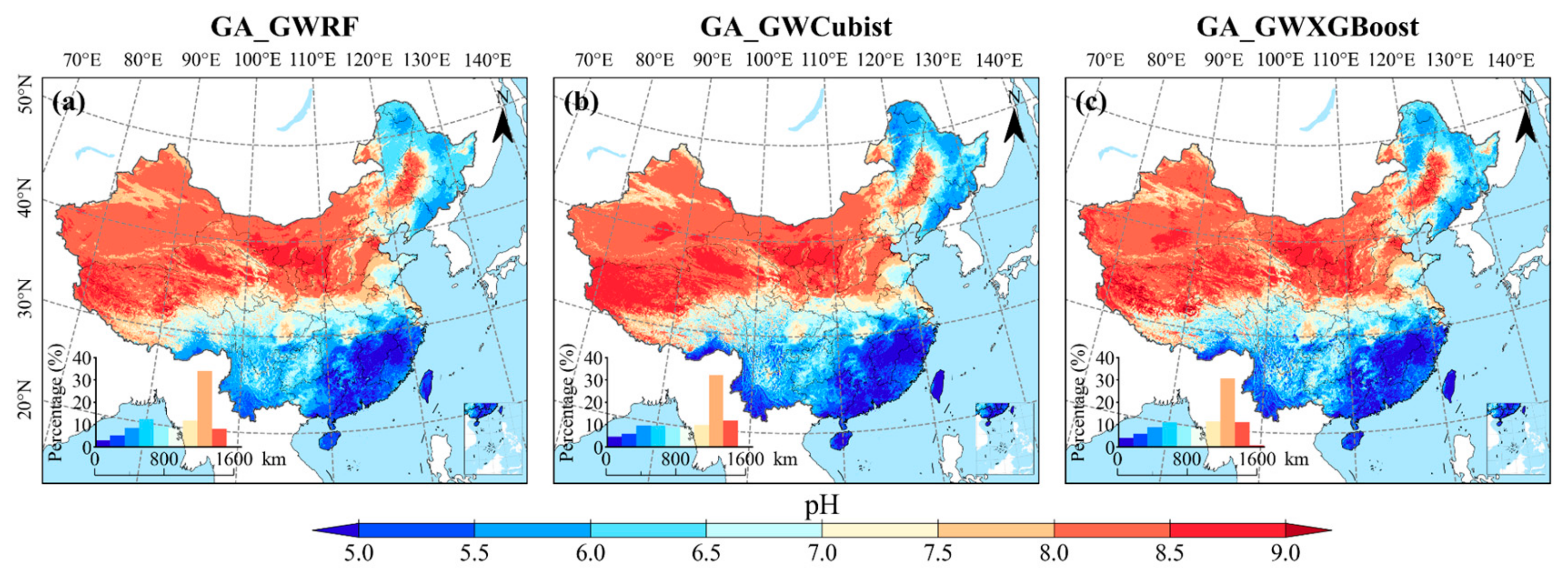
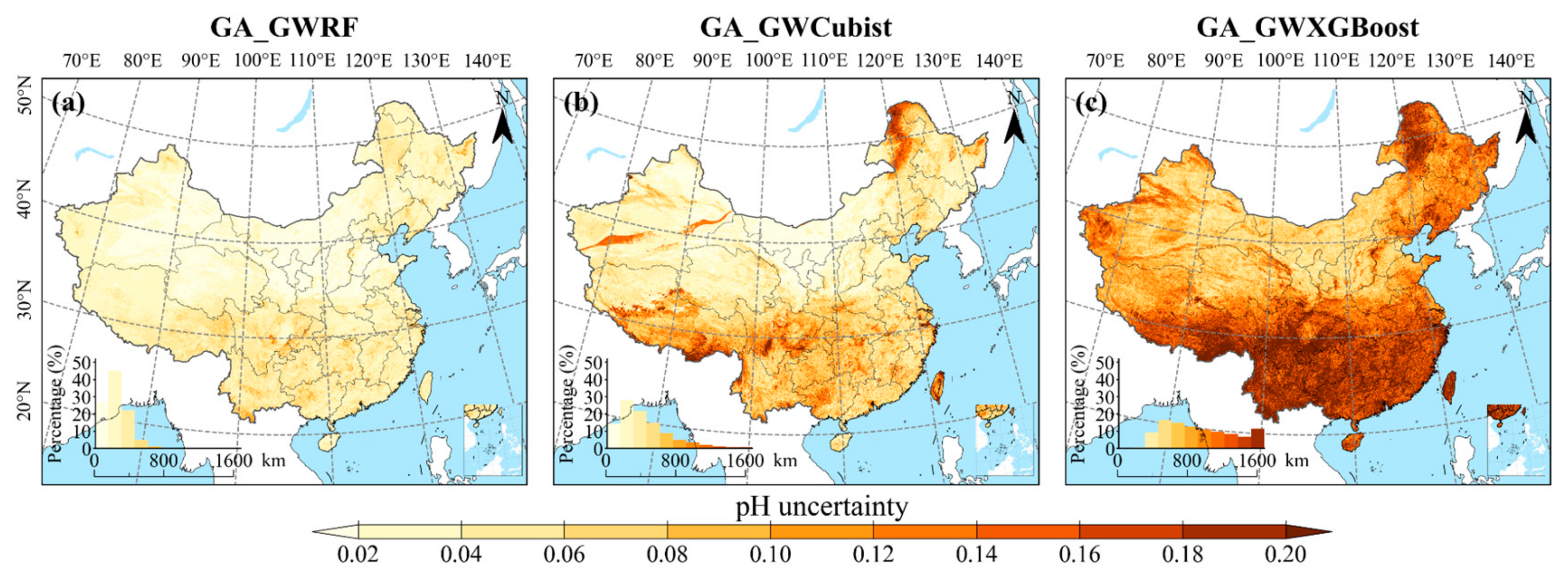
3.3. Spatial Patterns of the Predictions and Their Uncertainty

The appropriate semivariance model was selected on the basis of the maximum R² value (

Table 3. Geostatistical parameters of the models fitted to the experimental auto and cross-semivariograms.

Dataset	Fitted Models	Nugget (C0)	Sill (C0 + C)	Nugget Ratio (%)	Range (A0)/km	R2	RSS
All data	spherical	0.73	2.51	29.03	1878.00	0.99	0.04
train1	spherical	0.72	2.53	28.23	1872.00	0.99	0.04
train2	spherical	0.73	2.51	28.90	1880.00	0.99	0.04
train3	spherical	0.72	2.48	29.11	1840.00	0.99	0.04
train4	spherical	0.75	2.50	30.20	1868.00	0.99	0.04
train5	spherical	0.73	2.51	29.02	1880.00	0.99	0.04
train6	spherical	0.71	2.54	27.82	1889.00	0.99	0.05
train7	spherical	0.75	2.50	30.08	1897.00	0.99	0.03
train8	spherical	0.71	2.48	28.47	1837.00	0.99	0.04
train9	spherical	0.75	2.50	29.97	1905.00	0.99	0.03
train10	spherical	0.71	2.54	27.79	1911.00	0.99	0.04

). The spherical model best fits the experimental semivariogram of the pH, with the lowest residual sum of squares (RSS) value of 0.04 and the highest R² value of 0.99. The nugget ratio indicated that 29.03% of the variance was due to unexplained or random factors related to the soil pH. The spatial range of the soil pH (1878 km) was much larger than the average sampling interval, suggesting that the sampling system was adequate for determining the spatial distribution patterns of the soil pH. The optimal models of the 10 training sets were all spherical models, with parameters such as the nugget value, sill value, range, R^2, and residual value being close to those of the original dataset. This finding indicated that the 10 training sets provided satisfactory spatial representativeness. To further analyze the spatial aggregation effect of the soil pH, spatial autocorrelation analysis was conducted via Moran’s I (Figure 5). The soil pH exhibited a spatial clustering distribution of high and low values, and the soil pH showed significant spatial autocorrelation (Moran’s I = 0.69). This phenomenon indicates that spatial autocorrelation must be fully considered in the modeling of soil pH in order to more accurately reveal its spatial variability characteristics.

The soil pH maps generated with the different GWML models exhibited similar spatial variation trends with obvious banding characteristics (Figure 6). Regions with relatively high pH values were mainly located in Northwest China, North China, and Tibet, whereas areas with relatively low pH values were found in Central China, East China, South China, Northeast China, and Southwest China. However, local details varied between models, particularly in regions such as Xinjiang, Gansu, and Northeast China, where soil pH exhibited notable spatial heterogeneity. These differences suggest that model performance in different geographical regions may be closely related to differences in local soil properties and environmental factors. In addition, the pH values simulated by the GWML model in regions with sparse sample points exhibited significant spatial differences when compared to the GWR model (Figure S2a) and ML models (Figure S3). This indicates that the incorporation of geographically weighted regression plays a critical role in the prediction of soil pH in these areas.

The uncertainty in the prediction results was measured by the ratio of the median observations plotted within the 90% CI (Figure 7). There were significant spatial differences in the uncertainty maps obtained with the different GWML models. The GWRF model exhibited the lowest uncertainty among all models, followed by the GWCubist model. In contrast, the GWXGBoost model exhibited relatively higher uncertainties, particularly in regions with lower soil pH values, such as Central China, South China, and northern Northeast China, where it demonstrated the highest uncertainty.

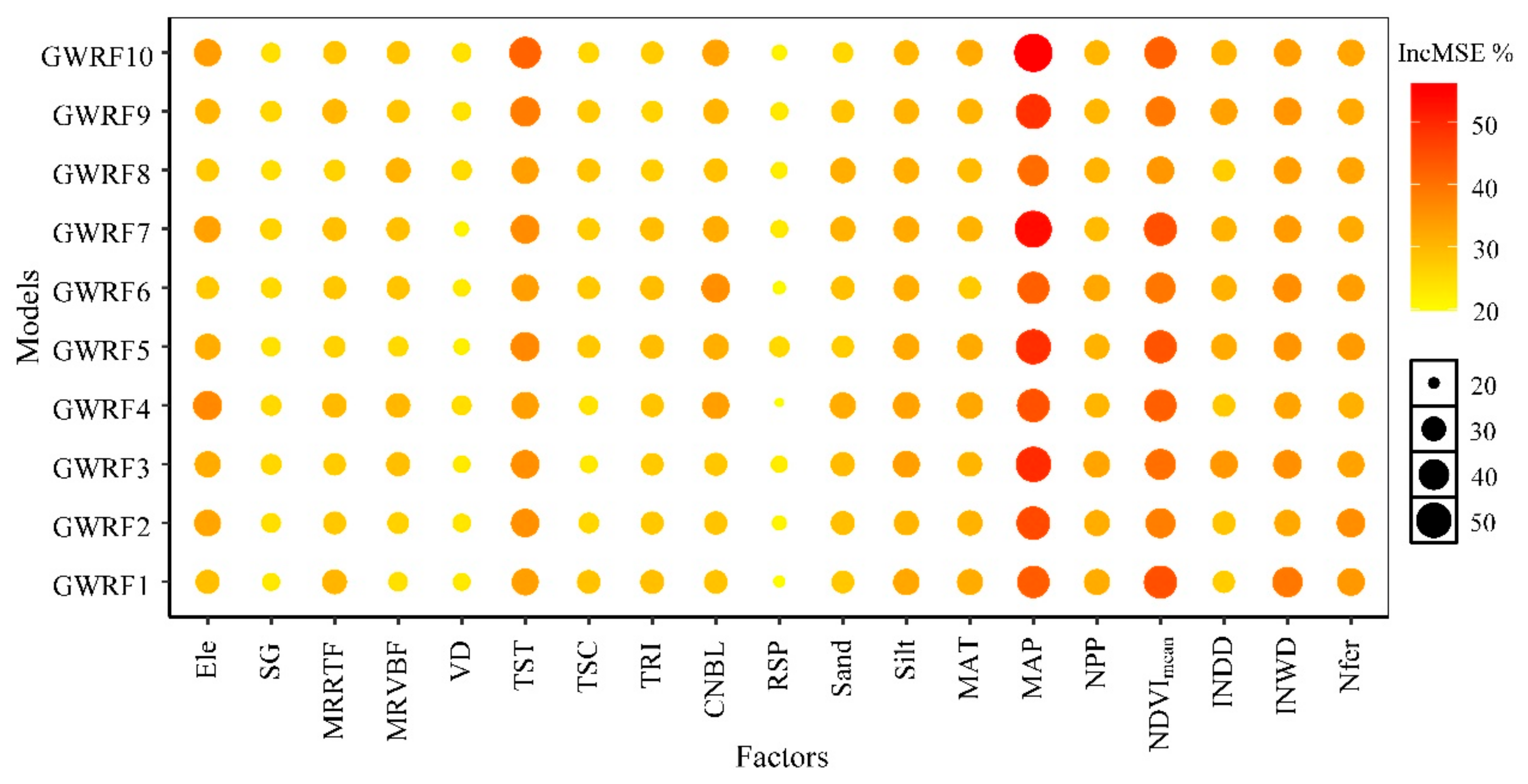
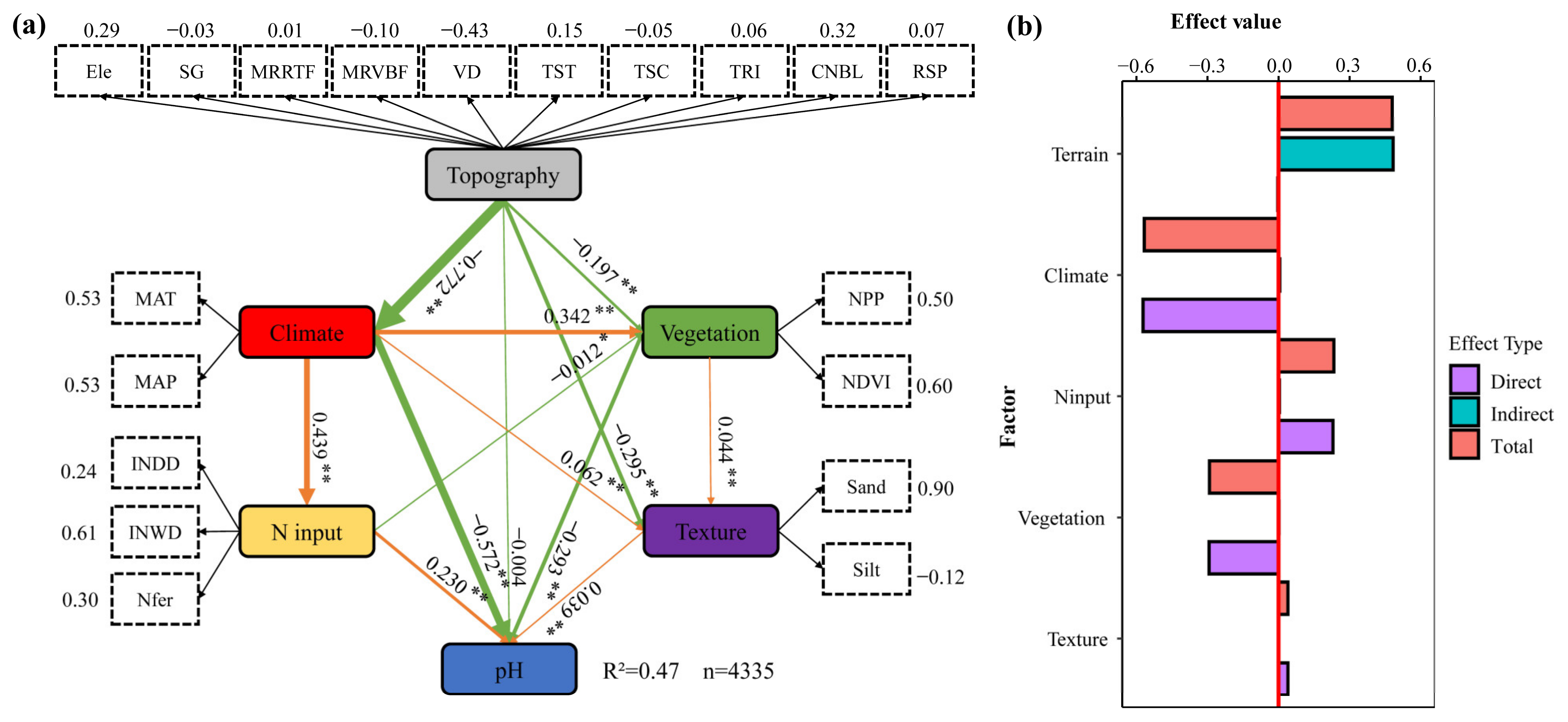
3.4. Environmental Controls on the Spatial Patterns of the Soil pH

The GWRF model was used to analyze the environmental covariates influencing the spatial patterns of the soil pH on the basis of the 19 covariates (Figure 8). The contributions of all covariates to soil pH prediction were similar among the different models, although their importance varied. The MAP, NDVI, and terrain surface texture (TST) were the three most important factors influencing the spatial pattern of soil pH.

In the partial least squares path modeling (PLS-PM) method, our conceptual framework significantly accounted for 47% of the total variation in the soil pH (Figure 9). The standardized path coefficients representing the effects of topography, climate, nitrogen input, vegetation, and soil texture on the soil pH were −0.004, −0.572, 0.230, −0.293, and 0.039, respectively. Apart from topography, all other factors significantly directly affected soil pH (p < 0.01). Overall, climate exerted the greatest influence on the soil pH, followed by nitrogen input and vegetation, whereas the soil texture yielded a relatively minor effect. Topography indirectly positively contributes to the soil pH by influencing climate and vegetation. Both climate and vegetation directly negatively affected the soil pH, with climate potentially influencing the soil pH indirectly by impacting vegetation and nitrogen inputs. Nitrogen inputs and soil texture directly contributed positively to the soil pH.

4. Discussion

4.1. Comparison of Contemporary Soil pH Mapping Assessments

Soil genesis theory states that similar soils can form under the same environmental conditions. The relationships between soil and the environment are complex, heterogeneous, and vary across different geographical regions [29]. Based on this, we combined GIS and remote sensing technologies to design and develop several GWML models optimized through the GA. In this study, we assessed the feasibility and improvements of these models in mapping soil pH across China. The result indicated that, compared to traditional GWR and ML models, the GWRF, GWCubist, and GWXGBoost models exhibited superior performance in soil pH prediction.

GWML models represent an extension of ML models in geographical analysis. The linear and nonlinear relationships between soil and the environment, as well as spatial nonsmoothness, are fully accounted for in the soil pH modeling process. Compared to traditional GWR and ML methods, the following enhancements were made. First, compared to the GWR model, GWML models exhibit a lower dependence on the number and distribution of sample points, which overcomes the local overfitting problem caused by sparse samples in the GWR model and increases the generalization ability of the model. Second, the existing ML model was improved with a spatial analysis module for each environmental factor across different geographic regions, which accurately captures the complex relationships between the soil and environment, enhances the interpretability of the model, and increases the prediction accuracy.

Among the three GWML models, the GWRF model exhibited the best prediction performance, followed by GWCubist and GWXGBoost. The performance differences can primarily be attributed to the characteristics and adaptability of the ML algorithms embedded in each model. RF effectively reduces the risk of overfitting by constructing multiple decision trees and using a voting mechanism to predict the outcome. It is particularly effective in handling complex and high-dimensional data, especially in soil pH prediction, where it accurately captures nonlinear relationships and interactions between variables. The Cubist model employs multiple linear regression models to describe the data and does not directly capture nonlinear relationships. Instead, it depends on rules and data partitioning to indirectly handle nonlinear features [31,32]. Compared to RF, it is less flexible, which constrains its ability to fit complex nonlinear patterns in the data. XGBoost, as a gradient-boosting tree model, improves the prediction performance step by step through a series of weak learners, thereby enhancing the overall prediction accuracy [33]. However, it is important to note that it may be an overfit in the region between the two peaks when dealing with bimodal data, leading to inaccurate predictions in the middle region. Additionally, its hyperparameter settings are more complex than those of RF and Cubist, requiring extensive tuning. This also explains the greater uncertainty in the prediction results for acidic soils.

The GWRF-based results showed varying degrees of improvement compared to previous studies (Figure 10). Compared to NSGC [16] and SoilGrids250m [14], this study achieved 13.74% and 56.27% reductions in RMSE and 2.46% and 53.68% increases in R², respectively. These findings further validate the effectiveness of the GWRF model in improving soil pH prediction accuracy. In addition, this study achieved a significant improvement in soil pH prediction accuracy compared to predictions derived from the spatial linking method. While the spatial connectivity approach facilitates the rapid generation of usable maps, it is susceptible to limitations regarding the scale of soil types, resulting in predictions that are inconsistent with the true values of the spatial variation in the soil pH [39]. DSM based on the GWRF model involves more sophisticated operations, utilizing abundant environmental data to accurately simulate the spatial variation in soil pH with relatively high mapping precision.

4.2. Spatial Distribution of Soil pH

The mean pH of topsoil in China was 6.83, which closely corresponds to the results reported by Zuo et al. [40] for the period between 2005 and 2014 (6.79). However, this value is significantly lower than the statistical results reported by Guo et al. [3] (6.92) and Chen et al. [12] (6.9) on the basis of the Second Soil Census (1979–1985). These findings suggested that topsoil acidification in China has intensified in recent years, potentially driven by agricultural practices, fertilization strategies, and environmental changes [41].

The decomposition of the semivariogram model reveals that the Nugget ratio of surface soil pH in China is 29.73%. This indicates that the spatial distribution of soil pH in China is influenced by both structural and random factors, with structural factors having a greater impact. The soil pH exhibits obvious spatial aggregation characteristics and shows a zonal distribution of acidity in the southern region and alkalinity in the northern region. The areas of acidic soils (pH < 6.5), neutral soils (6.5 ≤ pH < 7.5), and alkaline soils (pH ≥ 7.5) account for 29.52%, 14.44%, and 53.0 4%, respectively, of the total area. These findings highlight soil acidification and salinization as significant challenges in China.

A comparison of the soil pH distribution map generated in this study and those from previous research reveals that while both show similar spatial trends, there are significant differences at the local level (Figure 11). The findings underscore that different mapping methods introduce substantial uncertainty in soil pH spatial estimation, further emphasizing the necessity of advancing research on soil pH prediction methodologies.

4.3. Main Factors Influencing the Spatial Pattern of pH

The spatial variability in the soil pH is influenced by various factors, including topography, climate, parent material, vegetation cover, and anthropogenic activities [6,42,43]. This study revealed that climate has a significant negative impact on soil pH, which is consistent with the findings of Slessarev et al. [6]. Meanwhile, annual precipitation is an important environmental variable in soil pH prediction. Zhang et al. [20] and Chen et al. [12] also emphasized the importance of precipitation in soil pH prediction. In regions with a humi climates, the soil is usually acidic. Precipitation can carry acidic substances into the soil (such as acid rain), increasing the concentration of hydrogen ions (H⁺) in the soil, which lowers the soil pH and leads to soil acidification [44,45]. Moreover, precipitation further promotes soil acidification by leaching alkaline ions [46,47]. In addition, precipitation increases soil moisture, altering the biological activity of soil microorganisms and the chemical reaction processes in the soil, thus playing a key role in the acid-base balance of the soil. In arid regions, soil is predominantly alkaline. A higher evaporation-to-precipitation ratio leads to the upward movement of salt ions in the soil through capillary action, which exacerbates soil salinization [48,49].

The spatial pattern of vegetation is highly correlated with soil properties [50,51] and was used as a key variable in predicting soil pH [20,21]. In China, vegetation characteristics show significant spatial heterogeneity due to the diversity of climate, topography, and soil. In areas with high NDVI, soils are usually acidic. This is mainly due to organic acids secreted by plants through the root system or produced during the decomposition of vegetation residues entering the soil, increasing the acidity of the soil and lowering the pH. Additionally, as vegetations absorb cations (e.g., calcium, magnesium, and potassium) from the soil, they release hydrogen ions (H⁺), which further contribute to soil acidification. In contrast, in areas with low NDVI, the soil is usually alkaline. The vegetation cover in these areas is low, and in some areas, the ground is even bare, which directly affects the evaporation rate of surface water and promotes the accumulation of salts, potentially leading to soil alkalization. In addition, the impact of different types of vegetation on soil pH varies. Compared to grasslands and croplands, forests exhibit greater decomposition of plant residues and more intense root activity, which makes them more prone to inducing soil acidification [52]. Notably, soil pH and vegetation growth exhibit an interactive relationship. Excessively acidic or alkaline soils not only hinder plant nutrient uptake but also directly impact their growth and spatial distribution. Therefore, as a key indicator of vegetation growth and land use changes, NDVI serves as an essential tool for characterizing the spatial distribution of soil pH.

The application of chemical fertilizers and nitrogen deposition are major drivers of soil acidification [3,47]. Agricultural development in China is heavily dependent on nitrogen fertilizers, with excessive nitrogen input being the primary contributor to soil acidification in the region. Excess nitrogen sources deplete basic cations in the soil and disrupt the H⁺ cycle within the soil–plant system, thereby intensifying soil acidification [3]. Moreover, nitrogen compound emissions from the combustion of fossil fuels and intensive agricultural activities have increased atmospheric acid deposition and nitrogen deposition, which significantly impact soil pH. Interestingly, in this study, we found that nitrogen input exhibited a positive effect on soil pH. The contrasting result may be due to differences in fertilization practices, land use types, and climate conditions. In regions where excessive fertilization is not used, nitrogen input, through scientifically controlled timing and dosage, may help maintain or even increase soil pH rather than acidifying the soil. Additionally, this study covers multiple land use types, and the soil’s response to nitrogen input may vary across these different land uses. Compared to farmland soils, certain natural ecosystems (e.g., forests or grasslands) may have stronger buffering capacities, where moderate nitrogen input can promote plant and microbial activity, releasing alkaline substances that increase soil pH. Furthermore, we found that climate change has a positive promoting effect on nitrogen input. In arid regions, nitrogen deposition may be lower, so nitrogen input has less impact on soil pH. In contrast, in humid regions, nitrogen input may lead to more significant acidification effects. Excessive nitrogen input significantly increases autotrophic nitrification rates and promotes nitrate leaching, particularly under high precipitation conditions [53,54].

The influences of the lithology and geological background on soil pH mapping should not be overlooked [55]. Lithology is the basis for the physical and chemical properties of soil and significantly affects the range and distribution of soil pH. This study found that soil texture has a significant effect on the spatial distribution of soil pH. The response of soil pH change to additional input of acidic substances depends on the buffering capacity of the soil, which is closely related to soil texture. Loamy soils are susceptible to acidification, especially in the red soil areas of China, due to poor water permeability and weak buffering capacity, coupled with the accumulation of acids from the decomposition of organic matter, chemical fertilizers, and acids, and the effects of acidic precipitation. In sandy soils, on the other hand, the soil organic matter content is low, and the buffering capacity is poor, making them susceptible to acidification or alkalinization. In addition, clay and organic matter-rich soil exhibit greater resistance to pH fluctuations than sandy soils [56].

4.4. Limitations and Further Improvements

In large and complex regions, the relationship between soil pH and environmental factors is multifaceted, involving various interactions such as linear and nonlinear relationships as well as spatial correlations. These complexities pose significant challenges for DSM. In this study, we developed a hyperparameter-optimized GWML model to map the current spatial distribution of soil pH across China. While the results indicate that models such as GWRF, GWCubist, and GWXGBoost provide reasonable and acceptable estimates, there remain certain uncertainties and limitations that require further investigation.

Our study generated a 1 km × 1 km resolution soil pH map of China using multiple grid datasets closely associated with soil pH. However, the low resolution of certain parameters (e.g., nitrogen deposition and fertilizer application) may result in high uncertainty in the simulation outcomes. Thus, improving the accuracy of these grid parameters is crucial for enhancing model performance and map resolution. Another limitation is that, after comparing the performance of various GWML models, we selected the GWRF model as the optimal predictive choice. However, in large-scale regions with complex topography, relying solely on existing methods may not fully capture the intricate relationships between soil and environmental factors. Therefore, there is a need for continuous development of new DSM approaches to meet the diverse needs of different users and application scenarios, thereby providing more accurate and efficient technical support for land resource management, soil health assessment, and environmental protection.

Despite differences in model performance, each model exhibits unique strengths. By integrating the advantages of various models, a more accurate hybrid model can be constructed, enabling a more comprehensive capture of the spatial nonstationarity and nonlinear relationships between soil and the environment. With the continuous advancement of computational resources, the development and application of such super-models will not only improve the predictive accuracy of existing models but also open up new prospects for future soil science research and innovations in digital soil mapping technologies.

5. Conclusions

In this study, we combined GWR with three ML models (RF, Cubist, and XGBoost) and developed three GWML models optimized by GA to improve the prediction of soil pH. Compared with those of the GWR and traditional ML models, the prediction accuracies of the GWML models were significantly higher. Through a comprehensive comparison and evaluation of several models, we determined that the GWRF model provided the best prediction performance, and the soil pH map generated by this model exhibited high accuracy and reliability at large spatial scales. Furthermore, we analyzed the effects of climate, vegetation, nitrogen input, and soil texture on soil pH. The results showed that climate and vegetation had significant negative effects on soil pH, while nitrogen input and soil texture had significant positive effects. Our research addresses knowledge gaps in DSM methodologies at national and global scales and provides a new methodological reference for the Global Soil Mapping Network project. The soil pH map generated in this study provides critical data support for soil monitoring, agricultural optimization, and ecological protection, offering valuable scientific guidance for soil management and sustainable development strategies.

References

1. Minasny, B.; Hong, S.Y.; Hartemink, A.E.; Kim, Y.H.; Kang, S.S. Soil pH increase under paddy in South Korea between 2000 and 2012. Agric. Ecosyst. Environ. 2016, 221, 205–213. [Google Scholar] [CrossRef]
2. Minasny, B.; McBratney, A.B. Digital soil mapping: A brief history and some lessons. Geoderma 2016, 264, 301–311. [Google Scholar] [CrossRef]
3. Guo, J.H.; Liu, X.J.; Zhang, Y.; Shen, J.L.; Han, W.X.; Zhang, W.F.; Christie, P.; Goulding, K.W.T.; Vitousek, P.M.; Zhang, F.S. Significant acidification in major Chinese croplands. Science 2010, 327, 1008–1010. [Google Scholar] [CrossRef] [PubMed]
4. Zhao, Q.G. Nutrient Cycling in Red Soils and Their Management; Science Press: Beijing, China, 2002; pp. 137–145. [Google Scholar]
5. Liu, X.J.; Guo, K.; Feng, X.H.; Sun, H.Y. Discussion on the agricultural efficient utilization of saline-alkali land resources. Chin. J. Eco-Agric. 2023, 31, 345–353. [Google Scholar]
6. Kemmitt, S.; Wright, D.; Goulding, K.; Jones, D. pH regulation of carbon and nitrogen dynamics in two agricultural soils. Soil Biol. Biochem. 2006, 38, 898–911. [Google Scholar] [CrossRef]
7. McBratney, A.B.; Santos, M.M.; Minasny, B. On digital soil mapping. Geoderma 2003, 117, 3–52. [Google Scholar] [CrossRef]
8. Minasny, B.; McBratney, A.B.; Malone, B.P.; Wheeler, I. Digital mapping of soil carbon. Adv. Agron. 2013, 118, 1–47. [Google Scholar]
9. Zhang, G.L.; Liu, F.; Song, X.D. Recent progress and future prospect of digital soil mapping: A review. J. Integr. Agric. 2017, 16, 2871–2885. [Google Scholar] [CrossRef]
10. Jemejanova, M.; Kmoch, A.; Uuemaa, E. Adapting machine learning for environmental spatial data—A review. Ecol. Inform. 2024, 81, 102634. [Google Scholar] [CrossRef]
11. Were, K.; Bui, D.T.; Dick, Ø.B.; Singh, B.R. A comparative assessment of support vector regression, artificial neural networks, and random forests for predicting and mapping soil organic carbon stocks across an Afromontane landscape. Ecol. Indic. 2015, 52, 394–403. [Google Scholar] [CrossRef]
12. Chen, S.; Liang, Z.; Webster, R.; Zhang, G.; Zhou, Y.; Teng, H.; Hu, B.; Arrouays, D.; Shi, Z. A high–resolution map of soil pH in China made by hybrid modelling of sparse soil data and environmental covariates and its implications for pollution. Sci. Total Environ. 2019, 655, 273–283. [Google Scholar] [CrossRef]
13. Pouladi, N.; Møller, A.B.; Tabatabai, S.; Greve, M.H. Mapping soil organic matter contents at field level with Cubist, Random Forest and kriging. Geoderma 2019, 342, 85–92. [Google Scholar] [CrossRef]
14. Hengl, T.; De Jesus, J.M.; Heuvelink, G.B.M.; Gonzalez, M.R.; Kilibarda, M.; Blagotić, A.; Shangguan, W.; Wright, M.N.; Geng, X.; Bauer-Marschallinger, B.; et al. SoilGrids250m: Global gridded soil information based on machine learning. PLoS ONE 2017, 12, e0169748. [Google Scholar] [CrossRef] [PubMed]
15. Chagas, C.D.S.; Junior, W.D.C.; Bhering, S.B.; Calderano, F.B. Spatial prediction of soil surface texture in a semiarid region using random forest and multiple linear regressions. CATENA 2016, 139, 232–240. [Google Scholar] [CrossRef]
16. Liu, F.; Wu, H.Y.; Zhao, Y.G.; Li, D.C.; Yang, J.L.; Song, X.D.; Shi, Z.; Zhu, A.X.; Zhang, G.L. Mapping high resolution national soil information grids of China. Sci. Bull. 2022, 67, 328–340. [Google Scholar] [CrossRef]
17. Padarian, J.; Minasny, B.; McBratney, A.B. Machine learning and soil sciences: A review aided by machine learning tools. Soil 2019, 6, 35–52. [Google Scholar] [CrossRef]
18. Nussbaum, M.; Spiess, K.; Baltensweiler, A.; Grob, U.; Keller, A.; Greiner, L.; Schaepman, M.E.; Papritz, A. Evaluation of digital soil mapping approaches with large sets of environmental covariates. Soil 2017, 4, 1–22. [Google Scholar] [CrossRef]
19. Castrignanò, A.; Buttafuoco, G.; Comolli, R.; Castrignanò, A. Using Digital Elevation Model to Improve Soil pH Prediction in an Alpine Doline. Pedosphere 2011, 21, 259–270. [Google Scholar] [CrossRef]
20. Zhang, Y.; Sui, B.; Shen, H.O.; Wang, Z.M. Estimating temporal changes in soil pH in the black soil region of Northeast China using remote sensing. Comput. Electron. Agric. 2018, 154, 204–212. [Google Scholar] [CrossRef]
21. Ghazali, M.F.; Wikantika, K.; Harto, A.B.; Kondoh, A. Generating Soil Salinity, Soil Moisture, Soil pH from Satellite Imagery and Its Analysis. Inf. Process. Agric. 2020, 7, 294–306. [Google Scholar] [CrossRef]
22. Pahlavan-Rad, M.R.; Akbarimoghaddam, A. Spatial variability of soil texture fractions and pH in a flood plain (case study from eastern Iran). CATENA 2018, 160, 275–281. [Google Scholar] [CrossRef]
23. Haugen, H.; Devineau, O.; Heggenes, J.; Østbye, K.; Linløkken, A. Predicting habitat properties using remote sensing data: Soil pH and moisture, and ground vegetation cover. Remote Sens. 2022, 14, 5207. [Google Scholar]
24. Ye, M.; Zhu, L.; Li, X.; Ke, Y.; Huang, Y.; Chen, B.; Yu, H.; Li, H.; Feng, H. Estimation of the soil arsenic concentration using a geographically weighted XGBoost model based on hyperspectral data. Sci. Total Environ. 2023, 858, 159798. [Google Scholar] [CrossRef]
25. Fotheringham, A.S.; Brunsdon, C.A.; Charlton, M.E. Geographically Weighted Regression: The Analysis of Spatially Varying Relationships. Geogr. Anal. 2010, 35, 272–275. [Google Scholar]
26. Su, Z.W.; Lin, L.; Xu, Z.H.; Chen, Y.M.; Yang, L.M.; Hu, H.H.; Lin, Z.P.; Wei, S.J.; Luo, S.S. Modeling the effects of drivers on PM2.5 in the Yangtze River Delta with geographically weighted random forest. Remote Sens. 2023, 15, 3826. [Google Scholar] [CrossRef]
27. Zhang, G.L.; Wang, Q.B.; Zhang, F.R.; Wu, K.N.; Cai, C.F.; Zhang, M.K.; Li, D.C.; Zhao, Y.G.; Yang, J.L. Criteria for establishment of soil family and soil series in Chinese Soil Taxonomy. Acta Pedol. Sin. 2013, 50, 826–834, (In Chinese with English abstract). [Google Scholar]
28. Zhu, J.; He, N.; Wang, Q.; Yuan, G.; Wen, D.; Yu, G.; Jia, Y. The composition, spatial patterns, and influencing factors of atmospheric wet nitrogen deposition in Chinese terrestrial ecosystems. Sci. Total Environ. 2015, 511, 777–785. [Google Scholar] [CrossRef]
29. Jia, Y.; Yu, G.; Gao, Y.; He, N.; Wang, Q.; Jiao, C.; Zuo, Y. Global inorganic nitrogen dry deposition inferred from ground– and space–based measurements. Sci. Rep. 2016, 6, 19810. [Google Scholar] [CrossRef]
30. Yu, G.; Jia, Y.; He, N.; Zhu, J.; Chen, Z.; Wang, Q.; Piao, S.; Liu, X.; He, H.; Guo, X.; et al. Stabilization of atmospheric nitrogen deposition in China over the past decade. Nat. Geosci. 2019, 12, 424–429. [Google Scholar] [CrossRef]
31. Deng, S.; Li, Y.; Wang, J.; Cao, R.; Li, M. A feature-thresholds guided genetic algorithm based on a multi-objective feature scoring method for high-dimensional feature selection. Appl. Soft Comput. 2023, 148, 110765. [Google Scholar] [CrossRef]
32. Khaledian, Y.; Miller, B.A. Selecting appropriate machine learning methods for digital soil mapping. Appl. Math. Model. 2020, 81, 401–418. [Google Scholar] [CrossRef]
33. Zeraatpisheh, M.; Ayoubi, S.; Jafari, A.; Tajik, S.; Finke, P. Digital mapping of soil properties using multiple machine learning in a semi-arid region, central Iran. Geoderma 2019, 338, 445–452. [Google Scholar] [CrossRef]
34. Chen, T.; Guestrin, C. XGBoost: A scalable tree boosting system. In Proceedings of the 22nd ACM SIGKDD International Conference on Knowledge Discovery and Data Mining, San Francisco, CA, USA, 13–17 August 2016; pp. 785–794. [Google Scholar]
35. Wu, Z.F.; Sun, X.M.; Sun, Y.Q.; Yan, J.Y.; Zhao, Y.F.; Chen, J. Soil acidification and factors controlling topsoil pH shift of cropland in central China from 2008 to 2018. Geoderma 2022, 408, 115586. [Google Scholar] [CrossRef]
36. Arrouays, D.; Grundy, M.G.; Hartemink, A.E.; Hempel, J.W.; Heuvelink, G.B.; Hong, S.Y.; Lagacherie, P.; Lelyk, G.; McBratney, A.B.; McKenzie, N.J.; et al. GlobalSoilMap: Toward a fine-resolution global grid of soil properties. Adv. Agron. 2014, 125, 93–134. [Google Scholar]
37. Shangguan, W.; Dai, Y.; Liu, B.; Ye, A.; Yuan, H. A soil particle–size distribution dataset for regional land and climate modelling in China. Geoderma 2012, 171, 85–91. [Google Scholar] [CrossRef]
38. FAO.; ITPS. Status of the World’s Soil Resources: Main Report; Food and Agriculture Organization of the United Nations and Intergovernmental Technical Panel on Soils: Rome, Italy, 2015. [Google Scholar]
39. Liu, F.; Zhang, G.L.; Song, X.; Li, D.; Zhao, Y.; Yang, J.; Wu, H.; Yang, F. High–resolution and three–dimensional mapping of soil texture of China. Geoderma 2019, 361, 114061. [Google Scholar] [CrossRef]
40. Zuo, W.; Yi, S.; Gu, B.; Zhou, Y.; Qin, T.; Li, Y.; Shan, Y.; Gu, C.; Bai, Y. Crop residue return and nitrogen fertilizer reduction alleviate soil acidification in China’s croplands. Land Degrad. Dev. 2023, 34, 3144–3155. [Google Scholar] [CrossRef]
41. Xie, E.; Zhao, Y.; Li, H.; Shi, X.; Lu, F.; Zhang, X.; Peng, Y. Spatio–temporal changes of cropland soil pH in a rapidly industrializing region in the Yangtze River Delta of China, 1980–2015. Agric. Ecosyst. Environ. 2019, 272, 95–104. [Google Scholar] [CrossRef]
42. Geisseler, D.; Scow, K.M. Long-term effects of mineral fertilizers on soil microorganisms—A review. Soil Biol. Biochem. 2014, 75, 54–63. [Google Scholar] [CrossRef]
43. Cannone, N.; Guglielmin, M.; Malfasi, F.; Hubberten, H.W.; Wagner, D. Rapid soil and vegetation changes at regional scale in continental Antarctica. Geoderma 2021, 394, 115017. [Google Scholar] [CrossRef]
44. Kuang, F.; Liu, X.; Zhu, B.; Shen, J.; Pan, Y.; Su, M.; Goulding, K. Wet and dry nitrogen deposition in the central Sichuan Basin of China. Atmos. Environ. 2016, 143, 39–50. [Google Scholar] [CrossRef]
45. Zhao, Y.; Zhang, L.; Chen, Y.; Liu, X.; Xu, W.; Pan, Y.; Duan, L. Atmospheric nitrogen deposition to China: A model analysis on nitrogen budget and critical load exceedance. Atmos. Environ. 2017, 153, 32–40. [Google Scholar] [CrossRef]
46. Liu, X.J.; Mosier, A.R.; Halvorson, A.D.; Reule, C.A.; Zhang, F.S. Dinitrogen and N2O emissions in arable soils: Effect of tillage, N source and soil moisture. Soil Biol. Biochem. 2007, 39, 2362–2370. [Google Scholar] [CrossRef]
47. Tian, D.; Niu, S. A global analysis of soil acidification caused by nitrogen addition. Environ. Res. Lett. 2015, 10, 024019. [Google Scholar] [CrossRef]
48. Yu, J.; Li, Y.; Han, G.; Zhou, D.; Fu, Y.; Guan, B.; Wang, G.; Ning, K.; Wu, H.; Wang, J. The spatial distribution characteristics of soil salinity in coastal zone of the Yellow River Delta. Environ. Earth Sci. 2014, 72, 589–599. [Google Scholar] [CrossRef]
49. Peng, J.; Biswas, A.; Jiang, Q.; Zhao, R.; Hu, J.; Hu, B.; Shi, Z. Estimating soil salinity from remote sensing and terrain data in southern Xinjiang Province, China. Geoderma 2019, 337, 1309–1319. [Google Scholar] [CrossRef]
50. Liu, Z.P.; Shao, M.A.; Wang, Y.Q. Large–scale spatial interpolation of soil pH across the Loess Plateau, China. Environ. Earth Sci. 2013, 69, 2731–2741. [Google Scholar] [CrossRef]
51. Müller, T.S.; Dechow, R.; Flessa, H. Inventory and assessment of pH in cropland and grassland soils in Germany. J. Plant Nutr. Soil Sci. 2022, 185, 145–158. [Google Scholar] [CrossRef]
52. Zhang, Q.Y.; Zhu, J.X.; Wang, Q.F.; Xu, L.; Li, M.; Dai, G.H.; Mulder, J.; He, N.P. Soil acidification in China’s forests due to atmospheric acid deposition from 1980 to 2050. Sci. Bull. 2022, 67, 914–917. [Google Scholar] [CrossRef]
53. Wang, J.; Zhu, B.; Zhang, J.; Müller, C.; Cai, Z. Mechanisms of soil N dynamics following long–term application of organic fertilizers to subtropical rain–fed purple soil in China. Soil Biol. Biochem. 2015, 91, 222–231. [Google Scholar] [CrossRef]
54. Li, Q.; Luo, Y.; Wang, C.; Li, B.; Zhang, X.; Yuan, D.; Gao, X.; Zhang, H. Spatiotemporal variations and factors affecting soil nitrogen in the purple hilly area of Southwest China during the 1980s and the 2010s. Sci. Total Environ. 2016, 547, 173–181. [Google Scholar] [CrossRef] [PubMed]
55. Gray, J.M.; Bishop, T.F.; Wilford, J.R. Lithology and soil relationships for soil modelling and mapping. CATENA 2016, 147, 429–440. [Google Scholar] [CrossRef]
56. Fujii, K.; Hayakawa, C.; Panitkasate, T.; Maskhao, I.; Funakawa, S.; Kosaki, T.; Nawata, E. Acidification and buffering mechanisms of tropical sandy soil in northeast Thailand. Soil Tillage Res. 2017, 165, 80–87. [Google Scholar] [CrossRef]
Figure 1. Locations of the soil pH data across China (a). The distribution of soil pH data is based on Whittaker biomes, with elevation indicated by color (b).
Remotesensing 17 01086 g001
Figure 2. A methodological framework for soil pH mapping based on Genetic Algorithm-optimized GWML models.
Remotesensing 17 01086 g002
Figure 3. Distributions of the original pH (a) and the quantile transformer-processed pH (b).
Remotesensing 17 01086 g003
Figure 4. Scatterplot of the observed and predicted soil pH values in the validation set. (ac) represent different methods, which are the GA_GWRF, GA_GWCubist and GA_GWXGBoost models, respectively.
Remotesensing 17 01086 g004
Figure 5. Spatial distribution pattern of soil pH in China. The upper insets indicate the spatial self-phase of the soil pH. The four quadrants correspond to the four types of local spatial associations between regional units and their adjacent units, and quadrants 1–4 represent the high-high, high-low, low-low, and low-high clustering modes.
Remotesensing 17 01086 g005
Figure 6. Map of the spatial distribution of the soil pH. (ac) illustrate the map of soil pH using the GA_GWRF, GA_GWCubist and GA_GWXGBoost models, respectively.
Remotesensing 17 01086 g006
Figure 7. Uncertainties in the spatial distribution of soil pH. (ac) illustrate the uncertainty of soil pH values predicted using the GA_GWRF, GA_GWCubist and GA_GWXGBoost models, respectively.
Remotesensing 17 01086 g007
Figure 8. Degree of explanation of the different variables for the spatial distribution of the soil pH.
Remotesensing 17 01086 g008
Figure 9. Results of partial least square path modeling (PLS-PM) (a). The unidirectional cause-total effect between the six variables is shown as an arrow with a path coefficient (the orange and green arrows indicate positive and negative effects, respectively) (* p < 0.5; ** p < 0.01). The value above the arrow in the outer model is the weight of the measured variable. Direct, indirect, and total effects of five latent variables on the soil pH via PLS-PM (b).
Remotesensing 17 01086 g009
Figure 10. Comparison of our predictions (a) with the NSGC (b); the SoilGrids250m (c); the SPDC (d); and the HWSD2.0 values (e) over the 0–20 cm depth interval on the basis of the actual observed value samples.
Remotesensing 17 01086 g010
Figure 11. Soil pH maps from previous studies at depths from 0 to 20 cm. Map of the NSGC (a); the SoilGrids250m (b); the SPDC (c); and the HWSD2.0 data (d).
Remotesensing 17 01086 g011