Monitoring Leaf Rust and Yellow Rust in Wheat with 3D LiDAR Sensing

Abstract

Leaf rust and yellow rust are globally significant fungal diseases that severely impact wheat production, causing yield losses of up to 60% in highly susceptible cultivars. Early and accurate detection is crucial for integrating precision crop protection strategies to mitigate these losses. This study investigates the potential of 3D LiDAR technology for monitoring rust-induced physiological changes in wheat by analyzing variations in plant height, biomass, and light reflectance intensity. Results showed that grain yield decreased by 10–50% depending on cultivar susceptibility, with the durum wheat cultivar ‘Kiko Nick’ and bread wheat ‘Califa’ exhibiting the most severe reductions (~50–60%). While plant height and biomass remained relatively unaffected, LiDAR-derived intensity values strongly correlated with disease severity (R² = 0.62–0.81, depending on the cultivar and infection stage). These findings demonstrate that LiDAR can serve as a non-destructive, high-throughput tool for early rust detection and biomass estimation, highlighting its potential for integration into precision agriculture workflows to enhance disease monitoring and improve wheat yield forecasting. To promote transparency and reproducibility, the dataset used in this study is openly available on Zenodo, and all processing code is accessible via GitHub, cited at the end of this manuscript.

1. Introduction

Wheat is the third most produced cereal worldwide, behind corn and rice [1]. In terms of area planted and production, wheat is grown on almost all the planet’s surface except polar and equatorial zones [2]. According to the FAO database, its grain production reached approximately 780 million tons in 2023 annually [3]. However, according to Choudhary et al. [4], wheat production needs to increase by 2% annually in the coming years [5]. Further, the future global climate change scenarios and an estimated population of 9.6 billion by 2050 must be added together [6]. Furthermore, based on the literature review, wheat yields are, on average, approximately 20% lower than potential yields due to the effects of biotic (disease) and abiotic (drought) factors. In this context, a profit rate of approximately 2% per year is required to meet global food demands, but currently, only a 1% annual increase in yield has been reached [7,8]. With the large number of factors that can affect wheat production, fungal diseases (i.e., foliar and stem-base) have become the primary concern expressed by farmers [9].

Rusts are exceptionally destructive and among the various fungal diseases affecting wheat. Wheat cultivars susceptible to leaf rust often experience yield losses ranging from 5% to 15%, depending on the crop’s developmental stage. In cases where the variety is highly susceptible and weather conditions favor disease development, losses can reach as high as 60% [10]. One of the primary factors contributing to reduced wheat yields, with rust being particularly detrimental, is the indirect impact of rust on plant architecture, especially on leaves [11]. Infections typically coincide with the grain-filling stage, diminishing the interception and radiation absorption. This, in turn, leads to reduced assimilate supply per grain, resulting in a decrease in grain count, test weight, and alterations in the crop biomass. The current method for assessing disease occurrence relies on visual inspection by the human eye, which is effective when pustules are visible [12]. However, this inspection is constrained to specific areas, such as individual leaves, and does not provide comprehensive information about the entire crop architecture. Furthermore, visual evaluations are costly, time-consuming, and prone to error, as suggested by Nigus et al. [13], highlighting the need for a more reliable method to measure disease severity.

In the pursuit of more efficient crop monitoring methods, integrating remote-sensing technology into phenotyping techniques has emerged as an auspicious approach for the non-destructive measurement of crop parameters [14,15]. These innovative tools are particularly crucial as they facilitate a rapid acceleration of the breeding cycle, an advancement unprecedented in modern agriculture [16]. While molecular data are readily available, there is a notable gap in phenotypic data, which these remote phenotyping technologies aim to fill [17]. Breeders traditionally select leaf rust-resistant wheat cultivars by considering yield data and relying on their expertise—an approach constrained by its dependence on end-of-season outcomes, making it inherently slow. Recognizing this limitation, research has highlighted that leaf rust impacts yield and causes architectural changes in wheat plants, such as reduced biomass, shorter plant stature, and altered leaf orientation [18,19,20]. Given these insights, there is an apparent necessity for advanced techniques capable of early discrimination between wheat varieties based on their response to rust infection. Such techniques should enable the analysis of three-dimensional structural changes in plants from the earliest stages of infection, providing breeders with timely information to make informed decisions without waiting for the crop to reach maturity.

The characterization of plant architecture through 3D modeling has advanced significantly, with LiDAR technology becoming a key tool for extracting crop parameters [21,22]. Building on this progress, Shaoyong et al. [23] demonstrated the effectiveness of UAV-mounted LiDAR in accurately quantifying canopy structures. Using point cloud data captured by a LiDAR sensor, they applied the Simple Morphological Filter (SMRF) algorithm for ground removal and feature extraction to isolate the canopy, enabling precise estimation of canopy volume and estimate the canopy volume in a precise way. Although the application of LiDAR has been widespread, its use for monitoring leaf rust in wheat remains in the early stages. Minhui et al. [24] pioneered 3D data to enhance leaf rust detection, underscoring the method’s promise for crop health management.

Historically, sensors’ detection of wheat diseases has heavily depended on hyperspectral imaging techniques. Research by Whetton et al. [25] and Devadas et al. [26] has confirmed the effectiveness of these cameras in identifying diseases. Nonetheless, the practical application of hyperspectral imaging is limited by the substantial costs involved, which pose a financial challenge for low-margin crops like wheat. Another method for disease detection involves predictive models that use meteorological data [27]. Despite being a creative solution, these models have not consistently achieved the necessary accuracy for dependable disease prediction. The ongoing challenge is to strike an optimal balance between the cost-effectiveness and accuracy of disease monitoring techniques for wheat. Recent technological developments in LiDAR sensors, such as the Velodyne family, have the potential to provide not only 3D-point clouds but also near-infrared (NIR) intensity values, which can provide information comparable to spectral sensors, as mentioned by Gené-Mola et al. [28]. Lu et al. [29] have made similar recommendations regarding the usefulness of Velodyne sensor intensity readings, but no research has been performed to use the intensity values for rust detection.

Building on recent advancements in remote sensing, this study aims to develop an effective and non-destructive detection system for wheat rust using LiDAR technology. This system leverages the high precision and affordability of LiDAR sensors to identify leaf rust in durum wheat and yellow rust in bread wheat. While LiDAR has traditionally been employed for analyzing plant morphology—as demonstrated in previous studies on wheat canopy structure [19] and cucumber plant segmentation [21]—our work focuses on refining 3D point cloud applications for early rust detection. To achieve this, this study explores the correlation between LiDAR reflectance intensity and disease severity, evaluating how different intensity thresholds can serve as reliable indicators of infection. Additionally, we analyze structural changes in wheat plants, such as plant height and biomass variations, to assess their relationship with rust progression. Furthermore, we integrate statistical analyses, including standard deviation, standard error, ANOVA, and Pearson’s correlation coefficients, to validate the effectiveness of LiDAR-based metrics in distinguishing between resistant and susceptible cultivars. By combining 3D point cloud data, intensity-based analysis, and statistical validation, this system provides a cost-effective, scalable solution for disease monitoring. It offers breeders and farmers an efficient tool to assess rust severity before visible symptoms cause irreversible yield loss, supporting precision agriculture applications and improved disease management strategies. The results highlight the potential of LiDAR as an alternative to hyperspectral imaging, paving the way for its future implementation in large-scale wheat monitoring and disease detection frameworks.

2. Materials and Methods

2.1. Field Experiment Description

At the University of Seville in Spain, a controlled greenhouse experiment was conducted to evaluate the effects of rust infections on various wheat cultivars under semi-controlled conditions. Six wheat cultivars with different resistance levels were tested: three durum cultivars—‘Don Ricardo’ (resistant), ‘Amilcar’ (medium resistance), and ‘Kiko Nick’ (susceptible)—and three bread cultivars—‘Conil’ (resistant), ‘Arthur Nick’ (medium resistance), and ‘Califa’ (susceptible). Each cultivar was duplicated six times, yielding a total of 72 pots. Each three-liter pot was filled with a 60% peat and 40% sand substrate to reduce spatial bias and placed in a randomized arrangement. To avoid competition, plants were trimmed to one per pot 14 days after sowing (DaS) from an initial four seeds per pot. All plants were irrigated three times per week with 200 mL of water, while NPK (20–20–20) at a concentration of 2 g/L was applied three times during the growing season to ensure consistent nutrient availability. Greenhouse conditions were managed to minimize external stressors, and non-target diseases were monitored and treated as necessary.

At 78 DaS, inoculation was performed using a mini blower to disperse a mixture of uredospores and talcum powder (1:50 ratio, approximately 0.2 mg per genotype). While bread wheat plants were inoculated with yellow rust (Écija Jerezano 18, Warrior (-) race), durum wheat plants were inoculated with leaf rust (Conil Don Jaime 13, virulent to Lr14a). Following inoculation, bread wheat plants were incubated for 18 h at 20 °C, complete darkness, and 100% relative humidity to encourage rust attachment. On the other hand, durum wheat plants need a 24 h incubation period at 10 °C under complete darkness. Rust severity was assessed weekly from the week of inoculation until plant senescence using the modified Cobb scale, with the percentage of leaf area affected visually estimated [30]. Throughout the experiment, measurements were also made of the actual height of the plants (Aph). To assess the impact of rust on each cultivar, plants were harvested at 199 DaS, and important agronomic parameters such as biomass, number of ears, number of grains per plant, and total grain weight were collected.

2.2. Collection of Crop Parameters Information

At the end of the growing season, all inoculated and non-inoculated pots were harvested to measure various crop parameters that would serve as ground-truth data alongside the severity measurements taken on the specified days after inoculation (DAIs). The dry plants were cut at soil level in the pots, and their weight was measured using a scale; this weight was recorded as the biomass. Subsequently, the ears were collected individually to determine the number of ears (Noe), the number of grains (Nog), and the grain weight (Gw).

2.3. LiDAR Scanning of Wheat Plants for 3D Point Cloud Generation

The LiDAR Velodyne VLP-16 (Velodyne Lidar, Inc., San Jose, CA, USA) was used for 3D plant reconstruction. This high-precision 3D laser sensor features a rotating head equipped with multiple semiconductor lasers or laser diodes, each paired with its detector (Figure 1). The scanner was mounted at the front of the platform, positioned approximately 0.5 m above the crop canopy. The VLP-16 LiDAR sensor measures object reflectivity with 256-bit resolution, independent of laser power and distance, within a 1–100 m range. Absolute reflectivity calibration was performed using commercially available reflectivity standards stored in a calibration table within the sensor’s field-programmable gate array (FPGA). The VLP-16 scanner features 16 individual lasers and detectors arranged in a 30° field of view (FOV), providing a vertical resolution 2.0°. The sensor’s FOV is symmetrical relative to the horizontal plane, enabling point acquisition up to 100 m at a rate of approximately 300,000 points per second in single-return mode and 600,000 points per second in dual-return mode. The horizontal FOV spans 360°, with an adjustable rotation frequency ranging from 5 to 20 Hz. Due to the divergence of the laser beam, a single pulse can interact with multiple objects, resulting in multiple returns. The VLP-16 can analyze these multiple returns and report the strongest, last, or both (dual or dual mode) returns. Multiple returns occur when a laser pulse strikes the wheat plant at a location that does not completely obstruct the pulse path, allowing the remaining portion of the pulse to continue and interact with subsequent objects. One of the key features of this sensor is its ability to operate in the near-infrared (NIR) region at a wavelength of 903 nm [31]. This not only provides 3D information but also captures intensity values in a spectral region highly sensitive to changes in chlorophyll content. These intensity values will be used to estimate the severity of rust infection in wheat plants. To calibrate the intensity values from the crop, a calibrated white reference diffuse reflectance target (Spectralon® diffuse reflectance target, Labsphere, North Sutton, NH, USA), with dimensions of 127 × 127 mm and 99% reflectance was placed beside each plant.

An odometer system was integrated to ascertain the platform’s position, as depicted in Figure 2. This system was directly affixed to the wheel axle and featured an incremental optical encoder (Model E6B2-CWZ6C, OMRON Corporation, Kyoto, Japan). The rotary encoder generated 1000 pulses per revolution, offering a 1.8 mm resolution in the direction of platform movement. The cumulative pulse count from the odometer was collected using a low-cost open-hardware Arduino Nano V3.0 microcontroller (Arduino Project, Turin, Italy) programmed through the open-source Arduino Integrated Development Environment (IDE) version 1.8.19. After being collected by the microcontroller, the pulse data was transmitted to a computer via a USB interface, where it was synchronized with the LiDAR data to construct a 3D point cloud. These communication and computational processes were executed on an Ubuntu 18.04.5 LTS desktop workstation, and the Robot Operating System (ROS) Melodic (version 1.14.10) was employed for sensor control and data recording. The LiDAR point cloud data were stored in a bag file, a raw file format for storing ROS message data.

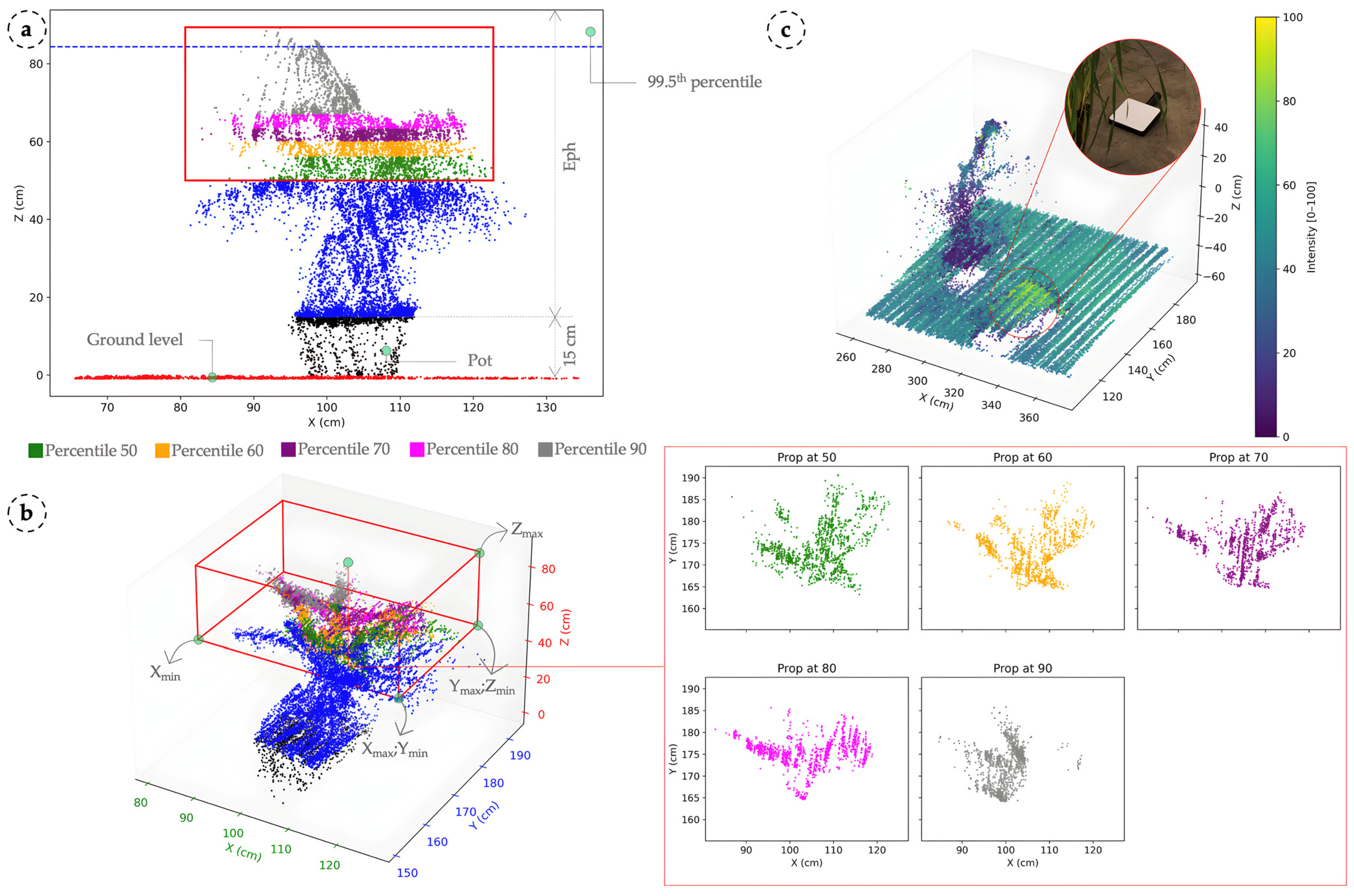
2.4. LiDAR-Based Analysis and Crop Parameter Extraction

After data collection, all the ROS bag files generated by the LiDAR sensor were converted into PCD (Point Cloud Data), executing the specific ROS commands. However, because PCD files are frequently stored in a binary format that can be hard to understand, they can occasionally be difficult to use. To solve this issue, a Python script was created to convert PCD files into CSV format. The GitHub version 3.16.0 repository at https://github.com/eapolo/agrolidarwheatrust (accessed on 1 January 2025) contains the code for manipulating point clouds, including the PCD-to-CSV conversion and test point cloud examples. The approach for parameter estimation is described below to compare the estimated crop parameters from LiDAR with ground-truth data. The aforementioned GitHub repository also has the code needed to access each parameter.

Eph (estimated plant height): it was calculated from the isolated plant point cloud using a robust percentile-based method to reduce noise and outliers. The initial step was to use a slope-based criterion to identify ground locations. The top 10% of these points were then chosen for reference plane fitting using Principal Component Analysis (PCA). The Z-coordinates of each point were normalized by subtracting the predicted ground level. Points below 0.15 m were not included because they matched the pot. The final plant height was calculated as the 99.5th percentile of the remaining Z-values (Equation (1)) to avoid measurement distortion caused by sensor noise or occasional outliers (Figure 3a).

$$Eph=P_{99.5}\left(Z\right)$$

(1)

where P_99.5 (Z) is the 99.5th percentile of the Z-coordinates.

Parea (estimated plant area): it was calculated using a rectangular box prism as a reference (Figure 3b), considering only points above the 50th percentile. This selection was made because rust symptoms primarily affect young leaves in the top canopy. Mathematically, the plant area was computed as the difference between the maximum and minimum X and Y coordinates within this selection (Equation (2)), which was then used to determine the plant’s breadth and length.

$${\mathit{P}}_{\mathit{a}\mathit{r}\mathit{e}\mathit{a}}=[\left(X_{max}-X_{min}\right)\times (Y_{max}-Y_{min}\left)\right]$$

(2)

Evol (estimated plant volume): the estimated plant volume was also computed using a bounding-box approach. The corresponding P_{area, i} was calculated for each percentile, and the maximum Z value within the points at that percentile (Z_{max, i}) was determined. The total Evol was then obtained as the sum of the products of P_{area, i} and Z_{max, i,} as described in Equation (3).

$${\mathit{E}}_{\mathit{v}\mathit{o}\mathit{l}}={\sum }_{i=1}^n{P}_{area,i}x{Z}_{max,i}$$

(3)

Prop50, Prop60, Prop70, Prop80, and Prop90 indicate how many points are in each percentile. This approach uses LiDAR data to model the plants with a certain percentage of the data points from the top to estimate plant volume.

The LiDAR-provided reflectance or intensity, which functions analogously to spectral sensors, was utilized to estimate severity. Intensity has been identified by Gené-Mola et al. [28] as a potential feature for segmenting fruit within the canopy of apple orchards. This investigation used the proportions of data points at each percentile to compute the mean reflectance. Thus, Int50, Int60, Int70, Int80, and Int90 were the investigated choices. A representative plant point cloud displaying the reflectance values is depicted in Figure 3c.

2.5. Statistical Analysis

The statistical analyses in this study were carried out using Python, version 3.11. The graphical plots illustrating the findings were also generated using this programming language. Linear correlation plots and matrix correlations employing Pearson’s r-value were utilized to evaluate the quality of the predictions. Lastly, we conducted a one-way analysis of variance (ANOVA) for every evaluated day after inoculation (DAI) to compare disease severity across cultivars at various periods. This test aimed to ascertain whether cultivar-to-cultivar variations in mean severity were statistically significant. We used Tukey’s Honest Significant Difference (HSD) post hoc test to determine which particular cultivar pairs showed significant differences if the ANOVA result was significant (p < 0.05), meaning that at least one cultivar varied from the others. A bar plot was used to visualize the results; statistically significant time points (based on ANOVA results) were shown with an asterisk (*), and mean severity values were shown with standard error bars. Using this method, we measured and contrasted cultivar susceptibility at various infection phases, giving us information about how resilient or vulnerable they were.

3. Results

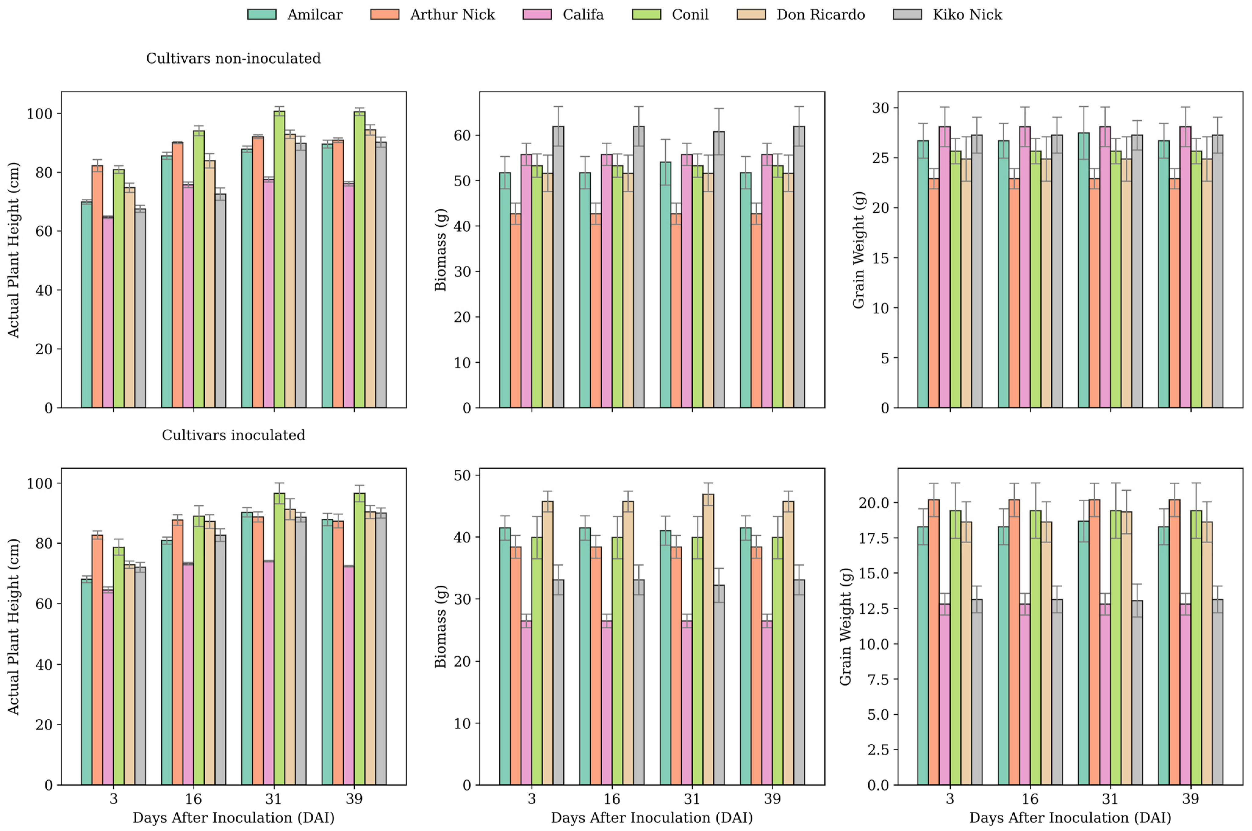
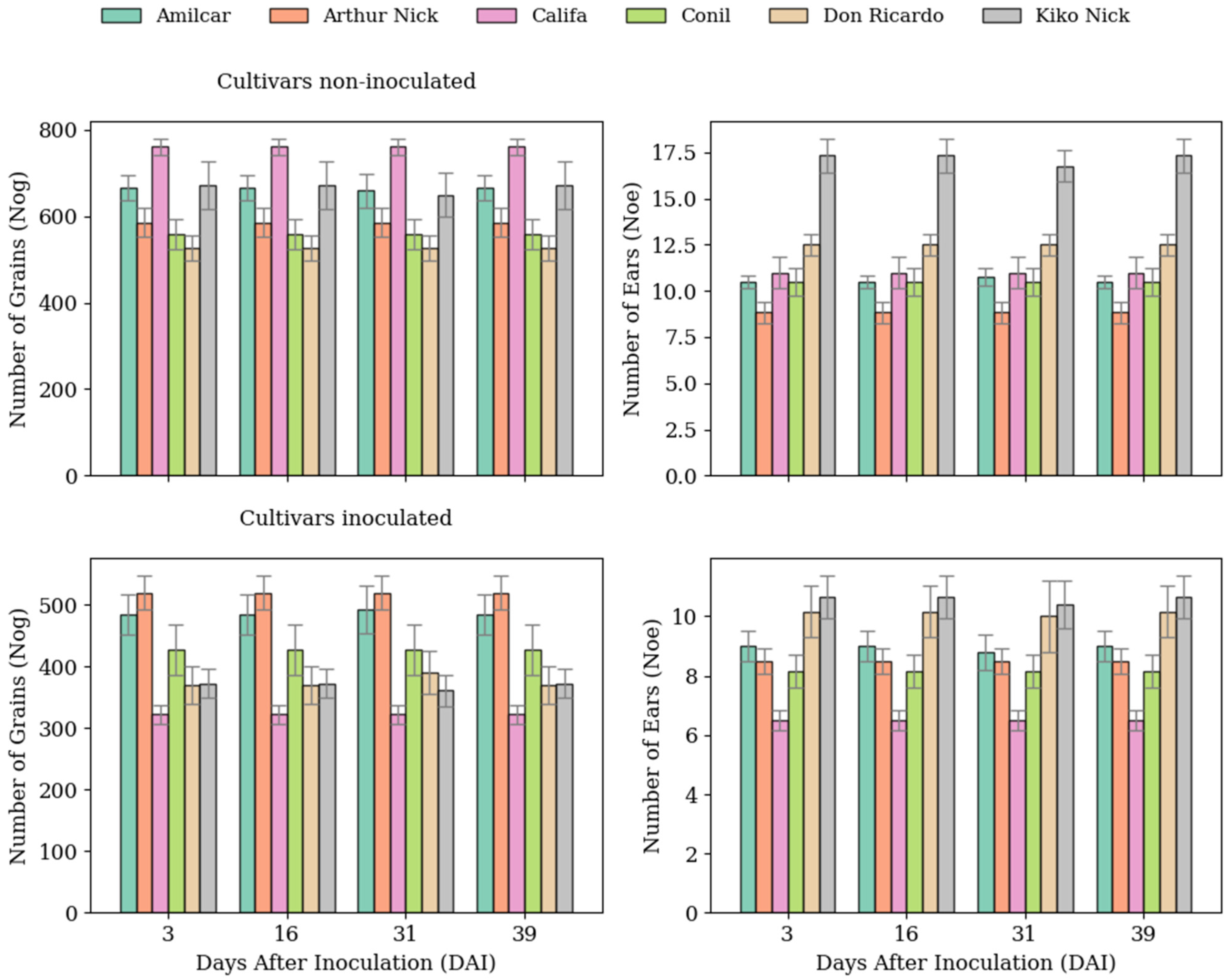
3.1. Ground-Truth Values Obtained Evolution

In Figure 4, no differences are observed in plant height and biomass parameters between plants inoculated with rust and their non-inoculated counterparts across resistant and susceptible varieties. This indicates that neither leaf nor yellow rust significantly impacts these growth parameters. Contrastingly, the grain production parameter (grain weight) significantly reduces, exceeding 50% in certain instances. This is particularly notable in the durum wheat cultivar ‘Kiko Nick’, which exhibits high susceptibility to leaf rust, and the bread wheat ‘Califa’, which is highly susceptible to yellow rust. Among the other durum wheat cultivars inoculated with leaf rust, ‘Don Ricardo’ exhibited an approximate 20% decrease in production, while ‘Amilcar’ suffered a loss of approximately 30%.

Similarly, among the bread wheat cultivars inoculated with yellow rust, ‘Arthur Nick’ incurred a production decrease of approximately 10%, and ‘Conil’ faced a reduction of approximately 20%. In Figure 3, it is observed that there is no difference in the parameters of plant height and biomass between inoculated and non-inoculated plants, neither in the resistant nor in the susceptible varieties. This confirms that both leaf and yellow rust do not affect these parameters. However, in terms of grain production (grain weight), there is a noticeable difference of more than 50% in production, especially in the durum wheat ‘Kiko Nick’, which is very susceptible to leaf rust, and the bread wheat ‘Califa’, which is very susceptible to yellow rust. On the other hand, the durum wheat ‘Don Ricardo’ and ‘Amilcar’ showed approximately 20% and 30% production loss, respectively, when inoculated with leaf rust. In the other bread wheat cultivars inoculated with yellow rust, ‘Arthur Nick’ experienced a loss of approximately 10%, and ‘Conil’ approximately 20% in production.

Figure 5 illustrates the impact of both leaf and yellow rust on the grain count per plant. In durum wheat cultivars that are resistant to leaf rust, such as ‘Amilcar’ and ‘Don Ricardo’, there was a decline in grain count exceeding 20%. In comparison, the susceptible variety ‘Kiko Nick’ experienced a nearly 50% reduction. Among the bread wheat varieties inoculated with yellow rust, the resistant cultivar ‘Arthur Nick’ exhibited a 10% decrease in grain number. The also resistant ‘Conil’ suffered a grain reduction of over 20%, while the susceptible ‘Califa’ faced a 60% reduction. Notably, the number of spikelets per ear is not as directly correlated with yield as the number of grains or grain weight. A plant susceptible to rust infection may produce smaller ears with fewer grains. Nonetheless, it has been noted that all cultivars, except ‘Arthur Nick’, showed a reduction in the number of spikelets per ear in the inoculated plants.

Figure 6 presents a bar chart that tracks the progression of the rust severity as a percentage over time, measured at intervals of 3, 16, 31, and 39 DAI across the six wheat cultivars. Initially, at 3 DAI, all cultivars exhibited relatively low disease severity, with ‘Amilcar’ and ‘Conil’ showing the lowest levels. As time progressed to 16 DAI, there was a noticeable increase in severity for all cultivars, with ‘Arthur Nick’ and ‘Kiko Nick’ experiencing a more pronounced rise. By 31 DAI, the severity had escalated further, with ‘Kiko Nick’ exhibiting the highest severity percentage, closely followed by ‘Arthur Nick’. ‘Califa’ and ‘Don Ricardo’ displayed moderate severity levels, while ‘Amilcar’ maintained the lowest severity among the cultivars. At the final measured interval of 39 DAI, the pattern of increasing severity continued, with ‘Kiko Nick’ still showing the most substantial severity. Notably, ‘Arthur Nick’ and ‘Califa’ significantly increased in severity, suggesting that these cultivars become more susceptible as the disease progresses. This pattern of progression is typical for rust infections, as Roelfs et al. [32] reported.

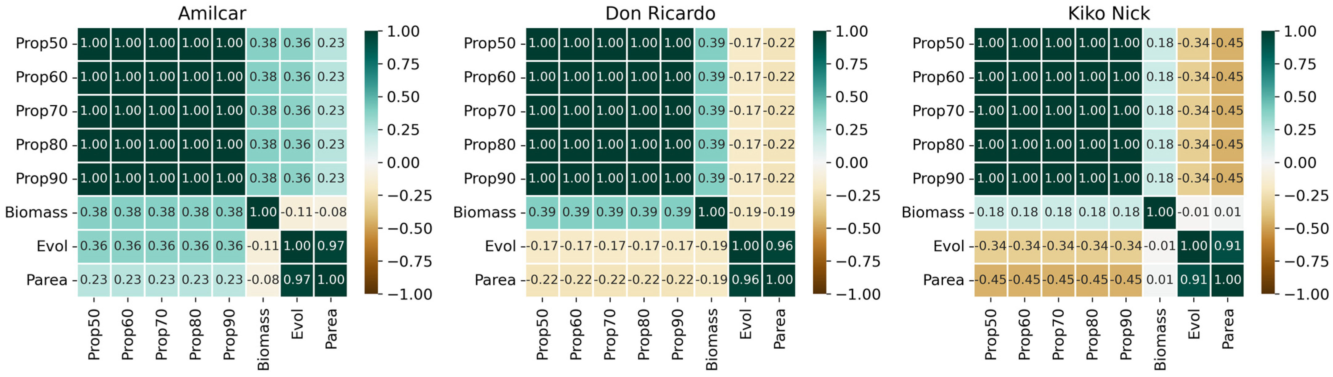
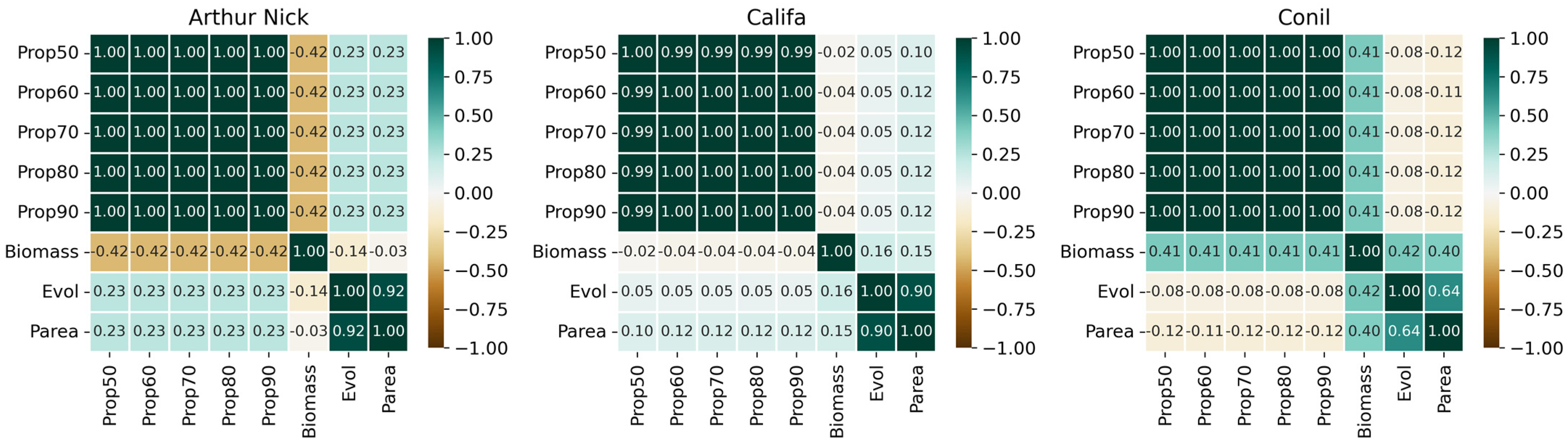
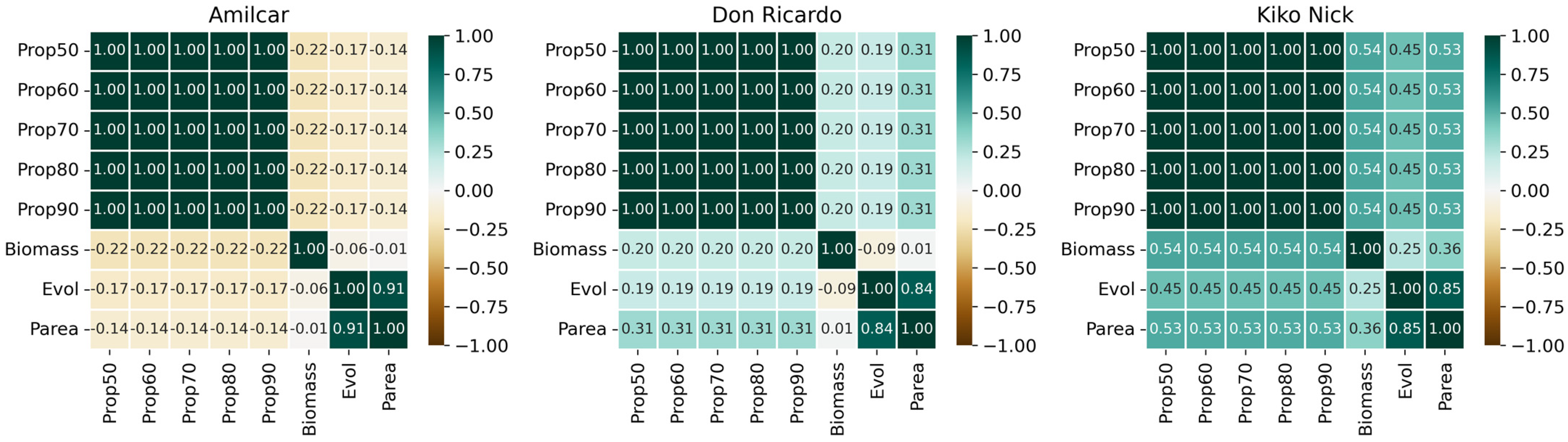
3.2. Correlations Between All the Crop Parameters Measured Manually and the Severity

This section analyzes correlations between crop parameters to determine their significance, focusing on traits influencing rust severity. Figure 7 presents correlation matrices for non-inoculated durum cultivars, revealing distinct trait interdependencies. In ‘Don Ricardo’, strong correlations exist between biomass and Gw (R² = 0.95) and biomass and Nog (R² = 0.92), emphasizing biomass accumulation as a key factor in yield formation. The near-perfect correlation between Gw and Nog (R² = 0.98) further underscores their interdependence. Conversely, ‘Amilcar’ shows weaker correlations, though biomass and Gw (R² = 0.93) and Gw and Nog (R² = 0.87) remain strongly linked, suggesting a more complex yield formation process. In both cultivars, correlations involving Aph are low (e.g., Aph and biomass, R² = 0.19 in ‘Amilcar’; Aph and Noe, R² = 0.30 in ‘Don Ricardo’), indicating a limited direct impact of aphids on yield-related traits. ‘Kiko Nick’ exhibits a more variable correlation structure, with biomass and Nog (R² = 0.97) showing the strongest relationship, reinforcing biomass’s role in grain production. Gw and biomass (R² = 0.89) are also strongly associated, while a moderate correlation between Noe and Gw (R² = 0.54) suggests that early plant establishment may modestly influence grain weight. The weak correlation between Aph and Noe (R² = −0.09) indicates minimal aphid impact on emergence.

Figure 8 presents heat maps of correlation patterns among crop parameters in non-inoculated bread wheat cultivars, highlighting distinct trait interdependencies. In ‘Arthur Nick’, growth-related traits show strong positive correlations, with biomass, Gw, and Nog nearly perfectly correlated (R² = 0.98–0.99), indicating a highly interrelated yield formation process. Noe also strongly correlates with Nog (R² = 0.99) and Gw (R² = 0.96), suggesting that early plant establishment significantly influences grain production. In contrast, Aph shows weak correlations (R² = 0.16–0.17), implying minimal impact on yield-related traits. ‘Califa’ displays generally moderate correlations, with the strongest observed between Gw and Nog (R² = 0.96), reinforcing their close association. Biomass also correlates strongly with these traits (R² = 0.91–0.93) but slightly less than in ‘Arthur Nick’. Noe shows moderate correlations with Nog (R² = 0.73) and Gw (R² = 0.68), while Aph consistently exhibits the weakest associations (e.g., Aph and biomass, R² = 0.13; Aph and Gw, R² = 0.11), indicating minimal influence of plant height on biomass accumulation and grain yield. In ‘Conil’, the strongest correlations occur between biomass and Nog (R² = 0.92) and Gw and Nog (R² = 0.92), highlighting their close interdependence. Noe also correlates well with biomass (R² = 0.77), suggesting that early plant establishment plays a more direct role in biomass accumulation. However, Aph shows weak or negative correlations with other traits (e.g., Aph and biomass, R² = −0.07; Aph and Nog, R² = −0.13), suggesting that plant height in this cultivar is largely independent of yield formation and may be influenced by other genetic or environmental factors.

Correlation heat maps for cultivars of inoculated durum wheat are shown in Figure 9, including disease severity as an extra metric to evaluate its association with important crop characteristics. In ‘Arthur Nick’, severity exhibits weak to moderate negative correlations with all parameters (e.g., Severity and Gw, R² = −0.20; Severity and biomass, R² = −0.26), suggesting a detrimental effect on growth and yield. Biomass and Gw maintain a strong positive correlation (R² = 0.95), consistent with non-inoculated plants. In ‘Califa’, severity shows no strong correlation with any trait (e.g., Severity and biomass, R² = −0.06; Severity and Gw, R² = 0.06), indicating minimal disease impact. However, Noe and Nog correlate strongly (R² = 0.91), highlighting a link between early plant establishment and grain production, though other relationships remain weaker. ‘Conil’ presents a distinct pattern, with severity showing mild negative correlations with biomass and Nog (R² = −0.10), suggesting a limited impact on yield. Unlike other cultivars, ‘Conil’ exhibits near-perfect correlations among biomass, Gw, and Nog (R² = 0.99–1.00), reinforcing biomass’s role in grain yield. Additionally, Aph correlates more strongly with biomass (R² = 0.69) and Gw (R² = 0.72) than other cultivars.

Figure 10 represents correlation matrices for the three bread wheat cultivars. In ‘Amilcar’, severity shows weak correlations with most traits, except for a moderate positive association with Noe (R² = 0.67), suggesting that disease pressure may influence ear number. Strong positive correlations between biomass and Gw (R² = 0.87) and biomass and Nog (R² = 0.69) confirm the expected link between biomass accumulation and yield. In ‘Don Ricardo’, severity exhibits strong negative correlations with Noe (R² = −0.85), biomass (R² = −0.55), Gw (R² = −0.51), and Nog (R² = −0.47), indicating a significant impact on plant establishment, biomass production, and yield. However, biomass, Gw, and Nog remain strongly interrelated (R² = 0.95–0.99), reinforcing their importance in yield formation. In ‘Kiko Nick’, severity weakly correlates with most traits but moderately associates with Aph (R² = 0.62), suggesting a possible link between disease pressure and plant height. Noe and Nog correlate moderately (R² = 0.79), while biomass, Gw, and Nog maintain strong interrelationships (R² = 0.84–0.93), suggesting that yield traits remain tightly linked despite some severity effects.

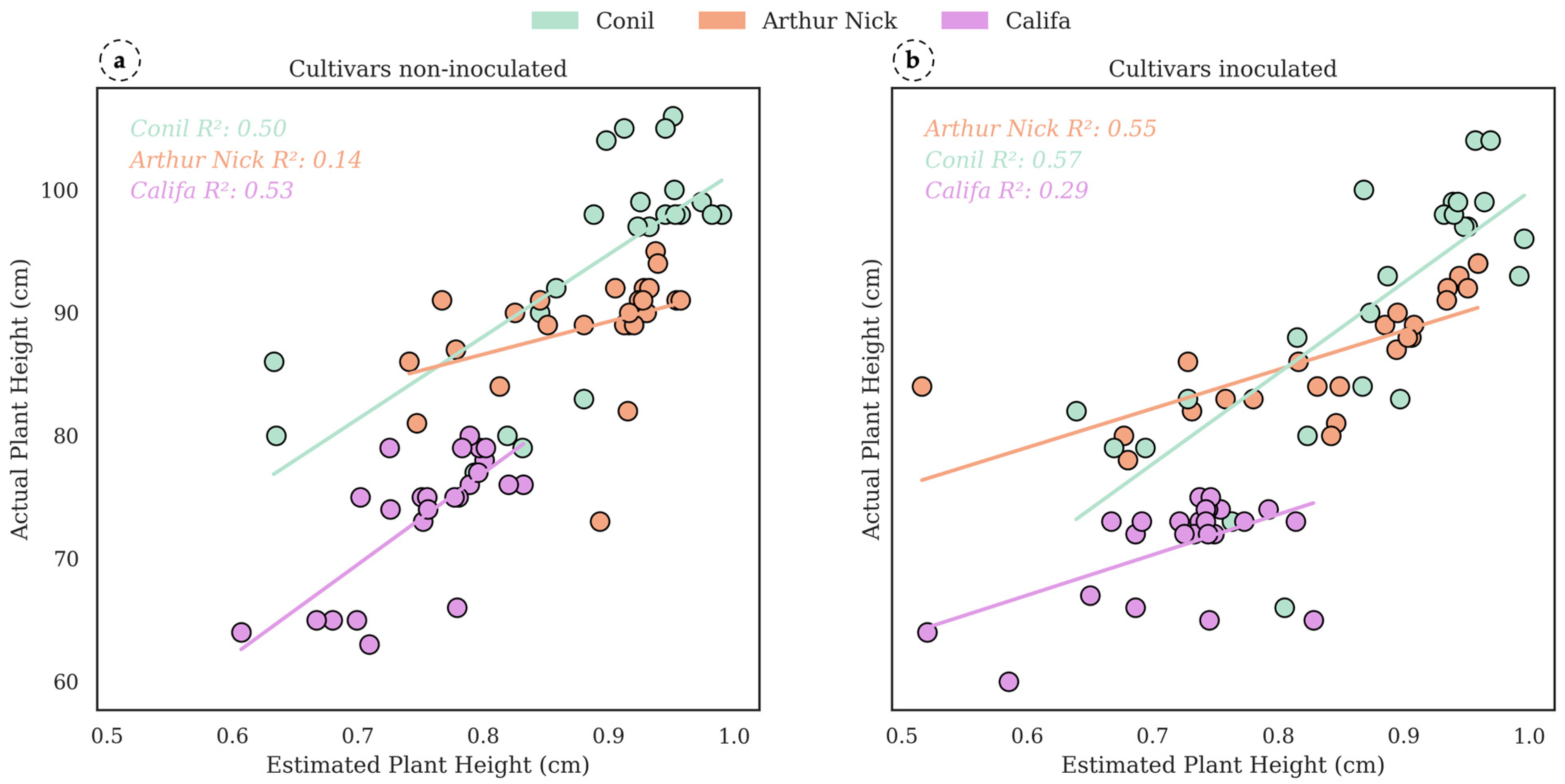
3.3. Estimation of Crop Parameters of Interest in Leaf Rust Detection

Section 3.2 examined the most relevant crop parameters associated with disease severity and those that can be readily derived from 3D point cloud data. This section presents findings on plant height and biomass estimation. Figure 11 illustrates the relationship between Aph and Eph across three bread wheat cultivars under both infected and non-inoculated conditions. In the non-inoculated panel, correlation strength varied: ‘Don Ricardo’ showed a low association (R² = 0.32), ‘Amilcar’ a moderate correlation (R² = 0.65), and ‘Kiko Nick’ the strongest predictive relationship (R² = 0.81). These differences suggest cultivar-specific accuracy in Eph’s estimation of Aph. On the other hand, in the inoculated panel, correlation patterns shifted. ‘Amilcar’ exhibited a weaker correlation (R² = 0.52), while ‘Kiko Nick’ and ‘Don Ricardo’ showed improved predictive strength (R² = 0.62 and R² = 0.63, respectively). The changes in R² values indicate that inoculation may affect the reliability of Eph in predicting actual plant height.

Expanding on the previous analysis, Figure 12 presents a regression analysis of actual Aph and Eph in bread wheat cultivars under non-inoculated and inoculated conditions. In the non-inoculated panel, ‘Califa’ (R² = 0.53) and ‘Conil’ (R² = 0.50) showed moderate correlations, while ‘Arthur Nick’ exhibited a weak association (R² = 0.14), indicating lower Eph accuracy. However, under inoculation, ‘Arthur Nick’ showed a significant improvement (R² = 0.55), ‘Conil’ had a slight increase (R² = 0.57), and ‘Califa’ declined (R² = 0.29), suggesting that inoculation affects the relationship between estimated and actual plant height in a cultivar-dependent manner. These findings align with Jiménez-Berni et al. [33], who used a LiDAR sensor to estimate wheat height, reinforcing the impact of inoculation on Eph accuracy.

Although biomass is not strongly correlated with disease severity, as mentioned in Section 3.2, this parameter is typically measured only at the end of the growing season. LiDAR data enable non-destructive estimation of biomass throughout the season. Furthermore, biomass is highly correlated with other parameters integral to determining final yield. Figure 13 illustrates heatmaps of Pearson’s correlation coefficients, showing relationships among estimated biomass (from 3D point cloud data at different percentiles), actual biomass, and additional parameters (Evol and Parea) in three durum wheat cultivars under non-inoculated conditions. Strong internal correlations among point cloud-derived biomass estimates reflect their shared structural basis, but their correlation with actual biomass remains low, highlighting challenges in accurate biomass prediction, especially during early growth stages. Correlations with Evol and Parea vary across cultivars, with weaker associations in ‘Amilcar’ and ‘Don Ricardo,’ while ‘Kiko Nick’ shows a stronger correlation between Parea and biomass, suggesting cultivar-specific influences. In some cases, negative correlations further emphasize the complexity of using 3D structural data for biomass estimation, underscoring the need for tailored approaches to improve accuracy across different wheat genotypes.

On the other hand, in Figure 14, the heat maps for non-inoculate bread wheat cultivars are depicted. In ‘Arthur Nick’, biomass correlations with estimated proportions are mostly weak to moderate, with some negative values, highlighting the limitations of 3D structural data for accurate biomass estimation. ‘Califa’ shows stable but weak correlations, suggesting that increasing captured data does not improve accuracy. In ‘Conil,’ biomass exhibits a significant negative relationship with predicted parameters, with Evol and Parea following the same trend, reinforcing cultivar-dependent variability in biomass estimation. These findings underscore the complexity of using 3D point clouds for biomass prediction in bread wheat and suggest that structural trait differences among cultivars play a key role in estimation accuracy.

Alighted with the previous description, in Figure 15 the results for inoculated durum wheat cultivars show clear trends in the accuracy of biomass estimation with the strongest connections found between biomass and Parea and Evol, ‘Kiko Nick’ shows modest relationships between real biomass and plant traits, indicating that structural features extracted from the 3D point cloud play a significant role in biomass prediction. Similar trends are seen in ‘Don Ricardo’; however, the correlations are often smaller. This suggests that although adding more point cloud data increases estimation accuracy somewhat, the link is still not as strong. ‘Amilcar’, on the other hand, exhibits weak to negative correlations between biomass and calculated parameters, indicating inconsistent efficacy of 3D structural data for biomass prediction in this cultivar. These results highlight how cultivar-specific characteristics affect biomass estimation and imply that plant design and inoculation response affect how well 3D point cloud data work.

The results for infected bread wheat cultivars show clear trends in biomass estimation accuracy in Figure 16. In ‘Conil,’ correlations between point cloud-derived estimates and actual biomass remain weak to moderate, showing slight improvement as data proportion increases, indicating persistent challenges in accurate biomass estimation. In contrast, ‘Califa’ shows stronger correlations, particularly between biomass, Parea, and Evol, suggesting that more detailed structural data enhances accuracy. ‘Arthur Nick’ exhibits a more consistent and positive correlation pattern across all proportions, especially with Evol and Parea indicating a stable relationship between estimated and actual biomass. These findings highlight the cultivar-dependent nature of biomass estimation and underscore the importance of plant structural traits in improving 3D point cloud-based models.

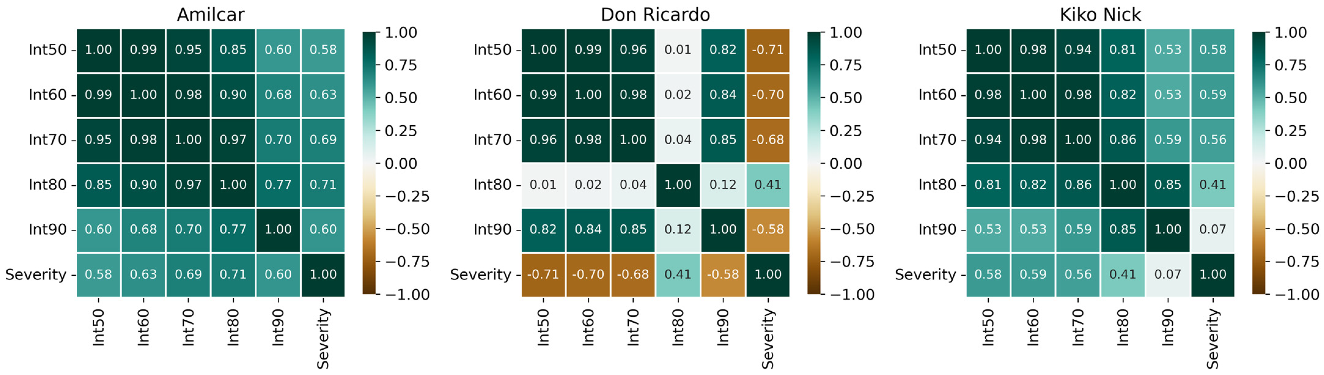
3.4. Severity Estimation

Heatmaps showing the relationship between LiDAR reflectance intensities and disease severity in three inoculated durum wheat cultivars are shown in Figure 17. The findings for ‘Kiko Nick’ show that severity and reflectance intensities have moderate relationships, with the strongest correlations occurring at lower intensity levels (Int50 and Int60), albeit these correlations diminish with increasing intensity. This implies that although some features of illness severity are captured by LiDAR intensity, the relationship is not highly linear. Because structural or physiological factors may influence reflectance, a clear negative connection exists between severity and all intensity levels in ‘Don Ricardo’, suggesting an inverse association where greater reflectance intensities correspond to lower severity values. On the other hand, ‘Amilcar’ regularly shows substantial positive associations at all intensity levels, indicating that LiDAR reflectance data better capture the degree of disease in this cultivar. These results underline the need for customized methods when employing remote sensing for disease assessment in wheat by highlighting cultivar-specific variations in the relationship between LiDAR intensity and disease severity.

Figure 18 illustrates the correlation between disease severity and LiDAR reflectance intensities for the three bread wheat cultivars. The results for ‘Conil’ indicate moderate correlations between reflectance intensity and disease severity, with a slight increase as more data points are included, suggesting that disease severity estimation benefits from higher intensity proportions, though the relationship remains relatively weak. In ‘Califa’, correlations between intensity and severity remain consistently low across all intensity levels, with no significant trend of improvement as more data points are incorporated, indicating that LiDAR reflectance may not effectively capture disease severity in this cultivar. In contrast, ‘Arthur Nick’ shows moderate correlations, with higher intensities (Int50 to Int80) exhibiting stronger relationships with severity, although a decline is observed at Int90. These findings highlight the variability in how LiDAR reflectance data correlate with disease severity across different cultivars, suggesting that factors such as canopy structure and disease distribution may influence the effectiveness of intensity-based severity estimation.

4. Discussion

4.1. LiDAR-Based Wheat Rust Severity Estimation Across Cultivars

Estimating wheat rust severity using LiDAR reflectance intensities offers a promising approach for precision agriculture, enabling timely and accurate disease monitoring. Our findings demonstrate that LiDAR-based severity assessments align with prior research [34,35], reinforcing its viability as a non-invasive tool for plant health evaluation.

Among the inoculated durum wheat cultivars, ‘Kiko Nick’ exhibited the strongest positive correlation between LiDAR reflectance intensities and disease severity, consistent with findings by Fahey et al. [36], who reported the utility of LiDAR in detecting foliar diseases due to the distinct light absorption and reflection properties of the rusted tissue. Similarly, ‘Amilcar’ maintained consistent correlations across intensity thresholds, indicating that even subtle reflectance changes effectively signal disease progression. For ‘Don Ricardo’, the emergence of significant correlations at higher intensity thresholds may suggest that the manifestation of disease symptoms is more discernible at advanced stages, where the spectral signature of the plant’s surface changes more noticeably. This delayed correlation is consistent with the findings by Khaled et al. [37], which indicated that the spectral detection of certain plant diseases becomes more reliable as symptoms become more pronounced. However, the relatively weaker correlations in ‘Conil’ and ‘Califa’ suggest that disease detection through LiDAR reflectance may be more complex, potentially influenced by factors such as the cultivar’s canopy structure or the disease’s spatial distribution within the field [38]. These discrepancies underscore the need for calibrating LiDAR-based severity estimation models to accommodate cultivar-specific and disease-specific factors, as Oblinger et al. [39] suggested. Moreover, the results corroborate the potential of LiDAR as a non-invasive method that can offer real-time data to farmers, enabling more precise applications of fungicides, leading to reduced chemical usage and associated costs [40]. Implementing LiDAR in integrated disease management programs could thus contribute to more sustainable agricultural practices [41].

Figure 19 illustrates the variation in mean LiDAR reflectance intensity across different percentile classes (Int50 to Int90), where the upper canopy layers (Int50, Int60) exhibit lower mean intensity values compared to lower sections (Int80, Int90). This trend suggests that biomass distribution, leaf density, and canopy structure significantly influence reflectance properties [42,43]. The increasing standard deviation at higher percentiles indicates more significant variability in reflectance, likely due to differences in light exposure and leaf arrangement at various canopy heights [44]. These insights reinforce the importance of considering structural canopy differences when integrating LiDAR-based severity models into precision agriculture [45,46].

4.2. Influence of Canopy Structure on LiDAR Reflectance Intensity

Table 1. Influence of biomass and actual plant height (Aph) on severity estimation across wheat cultivars. Values are regression coefficients, where negative biomass indicates reduced accuracy in intensity-based severity estimation, and positive Aph suggests improved prediction.

Wheat Type	Cultivars	Biomass Influence	Aph Influence
Durum	‘Don Ricardo’	−0.2556	0.0118
	‘Kiko Nick’	−0.7509	2.2690
	‘Amilcar’	−1.0070	1.1495
Bread	‘Conil’	−0.5753	1.0719
	‘Arthur Nick’	−1.1679	0.2611
	‘Califa’	−2.5226	−6.2537

illustrates how cultivar-specific variations in biomass and pH influence the connection between wheat rust severity and intensity-based estimates (Int50–Int90). We used a multiple linear regression model to assess this effect, predicting severity based on intensity levels while considering Aph and biomass. The biomass and Eph model coefficients show how they affect the severity-intensity relationship. Though resistant cultivars like ‘Don Ricardo’ (−0.25) and ‘Conil’ (−0.57) were less impacted, biomass consistently decreased estimation accuracy, with the biggest negative effect seen in ‘Califa’ (−2.52) and ‘Amilcar’ (−1.00). This implies that higher biomass modifies disease progression in susceptible and medium-resistant cultivars, reducing the accuracy of intensity-based predictions. However, in sensitive cultivars, Aph had a favorable effect on severity assessment (‘Kiko Nick’: 2.26, ‘Amilcar’: 1.15, ‘Conil’: 1.07), suggesting that it may be used as an early disease indicator. Aph, however, had little effect on resistant cultivars (‘Don Ricardo’: 0.01) because these types inherently slow the spread of disease. Interestingly, the inverse Aph effect in ‘Califa’ (−6.25) indicated that the cultivar’s rust severity and Aph levels were out of sync. When wheat types were pooled, ‘durum’ wheat showed a more significant negative biomass effect (−1.85) than bread wheat (−0.87). This finding aligns with Shafi et al. [47], who reported that structural differences in wheat canopies influence disease detection, requiring additional physiological parameters for accurate severity estimation in durum varieties. In contrast, bread wheat showed greater stability in intensity-based severity models, indicating that spectral reflectance alone may provide more reliable disease monitoring in these cultivars. Zheng et al. [48] found that structural changes in the canopy due to vegetation infection become more pronounced in the mid-late growth stage, reinforcing the importance of integrating spectral and physiological characteristics into future models for more precise wheat disease monitoring.

5. Conclusions

Concluding this study, it is evident that leaf and yellow rust infection significantly impacts grain weight across various wheat cultivars, with notable reductions exceeding 50% in highly susceptible varieties. This effect is less pronounced on growth parameters such as plant height and biomass, which remain relatively unaffected by rust infection. The strong correlations observed between actual biomass and larger proportions of 3D point cloud data underscore the potential of LiDAR technology for non-destructive biomass estimation. However, the accuracy of these predictions varies among cultivars and is contingent upon the developmental stage, highlighting the need for cultivar-specific calibration. Moreover, disease severity can be reliably assessed using LiDAR reflectance intensities, mainly when larger datasets are analyzed, demonstrating the technology’s utility in precision agriculture for disease monitoring and management. Overall, integrating 3D point cloud data presents a promising avenue for enhancing crop parameter estimation and disease severity assessment, thereby supporting informed decision-making in crop management.

While applying LiDAR technology for severity estimation is promising, it is imperative to consider the variability among different wheat cultivars and the stages of disease progression. Future studies should focus on refining the estimation models and exploring integrating LiDAR data with other remote sensing modalities to enhance the accuracy and reliability of disease severity assessments. These advancements will further solidify LiDAR’s role in precision agriculture, contributing to more effective disease monitoring strategies and improved crop management.

References

1. Igrejas, G.; Ikeda, T.M.; Guzmán, C. Wheat Quality for Improving Processing and Human Health; Springer International Publishing: Berlin/Heidelberg, Germany, 2020; ISBN 9783030341633. [Google Scholar]
2. Le Gouis, J.; Oury, F.X.; Charmet, G. How Changes in Climate and Agricultural Practices Influenced Wheat Production in Western Europe. J. Cereal Sci. 2020, 93, 102960. [Google Scholar] [CrossRef]
3. FAO (Food and Agriculture Organization). Crop Prospects and Food Situation—Triannual Global Report No. 3, November 2023; FAO: Rome, Italy, 2023. [Google Scholar] [CrossRef]
4. Choudhary, M.; Yadav, M.; Get, S.; Saran, R. Advanced Screening and Breeding Approaches for Heat Tolerance in Wheat. J. Pharmacogn. Phytochem. 2020, 9, 1047. [Google Scholar]
5. Jasrotia, P.; Lal Kashyap, P.; Kumar Bhardwaj, A.; Kumar, S.; Pratap Singh, G.; Kashyap, P.; Bhardwaj, A.; Kumar, S.; Singh, G. Wheat and Barley Research Scope and Applications of Nanotechnology for Wheat Production: A Review of Recent Advances Article History Citation Scope and Applications of Nanotechnology for Wheat Production: A Review of Recent Advances. Wheat Barley Res. 2018, 10, 1–14. [Google Scholar] [CrossRef]
6. Bahar, N.H.A.; Lo, M.; Sanjaya, M.; Van Vianen, J.; Alexander, P.; Ickowitz, A.; Sunderland, T. Meeting the Food Security Challenge for Nine Billion People in 2050: What Impact on Forests? In Global Environmental Change; Elsevier Ltd.: Amsterdam, The Netherlands, 2020; Volume 62. [Google Scholar] [CrossRef]
7. De La Fuente, G.N.; Frei, U.K.; Lübberstedt, T. Accelerating Plant Breeding. Trends Plant Sci. 2013, 18, 667–672. [Google Scholar] [CrossRef] [PubMed]
8. Ray, D.K.; Mueller, N.D.; West, P.C.; Foley, J.A. Yield Trends Are Insufficient to Double Global Crop Production by 2050. PLoS ONE 2013, 8, e66428. [Google Scholar] [CrossRef]
9. Vergara-Diaz, O.; Kefauver, S.C.; Elazab, A.; Nieto-Taladriz, M.T.; Araus, J.L. Grain Yield Losses in Yellow-Rusted Durum Wheat Estimated Using Digital and Conventional Parameters under Field Conditions. Crop J. 2015, 3, 200–210. [Google Scholar] [CrossRef]
10. Kolmer, J.A.; Hughes, M.E. Physiologic Specialization of Puccinia triticina on Wheat in the United States in 2016. Plant Dis. 2018, 102, 1066–1071. [Google Scholar] [CrossRef]
11. Yuan, W.; Li, J.; Bhatta, M.; Shi, Y.; Baenziger, P.S.; Ge, Y. Wheat Height Estimation Using LiDAR in Comparison to Ultrasonic Sensor and UAS. Sensors 2018, 18, 3731. [Google Scholar] [CrossRef]
12. Kumar, D.; Kukreja, V. Deep Learning in Wheat Diseases Classification: A Systematic Review. Multimed. Tools Appl. 2022, 81, 10143–10187. [Google Scholar] [CrossRef]
13. Nigus, E.A.; Taye, G.B.; Girmaw, D.W.; Salau, A.O. Development of a Model for Detection and Grading of Stem Rust in Wheat Using Deep Learning. Multimed. Tools Appl. 2024, 83, 47649–47676. [Google Scholar] [CrossRef]
14. Winterhalter, L.; Mistele, B.; Schmidhalter, U. Evaluation of Active and Passive Sensor Systems in the Field to Phenotype Maize Hybrids with High-Throughput. Field Crops Res. 2013, 154, 236–245. [Google Scholar] [CrossRef]
15. Araus, J.L.; Cairns, J.E. Field High-Throughput Phenotyping: The New Crop Breeding Frontier. Trends Plant Sci. 2014, 19, 52–61. [Google Scholar] [CrossRef] [PubMed]
16. Yao, Z.F.; He, D.J.; Lei, Y. Thermal Imaging for Early Nondestructive Detection of Wheat Stripe Rust. In Proceedings of the ASABE 2018 Annual International Meeting, Detroit, MI, USA, 29 July–1 August 2018; American Society of Agricultural and Biological Engineers: St. Joseph, MI, USA, 2018. [Google Scholar] [CrossRef]
17. Montes, J.M.; Technow, F.; Dhillon, B.S.; Mauch, F.; Melchinger, A.E. High-Throughput Non-Destructive Biomass Determination during Early Plant Development in Maize under Field Conditions. Field Crops Res. 2011, 121, 268–273. [Google Scholar] [CrossRef]
18. Jay, S.; Rabatel, G.; Hadoux, X.; Moura, D.; Gorretta, N. In-Field Crop Row Phenotyping from 3D Modeling Performed Using Structure from Motion. Struct. Motion. Comput. Electron. Agric. 2015, 110, 70–77. [Google Scholar] [CrossRef]
19. Li, L.; Ma, Z.; Niinemets, Ü.; Guo, D. Three Key Sub-Leaf Modules and the Diversity of Leaf Designs. Front. Plant Sci. 2017, 8, e01542. [Google Scholar] [CrossRef] [PubMed]
20. Holman, F.H.; Riche, A.B.; Michalski, A.; Castle, M.; Wooster, M.J.; Hawkesford, M.J. High Throughput Field Phenotyping of Wheat Plant Height and Growth Rate in Field Plot Trials Using UAV Based Remote Sensing. Remote Sens. 2016, 8, 1031. [Google Scholar] [CrossRef]
21. Boogaard, F.P.; van Henten, E.J.; Kootstra, G. Boosting Plant-Part Segmentation of Cucumber Plants by Enriching Incomplete 3D Point Clouds with Spectral Data. Biosyst. Eng. 2021, 211, 167–182. [Google Scholar] [CrossRef]
22. Rebetzke, G.J.; Jimenez-Berni, J.; Fischer, R.A.; Deery, D.M.; Smith, D.J. Review: High-Throughput Phenotyping to Enhance the Use of Crop Genetic Resources. Plant Sci. 2019, 282, 40–48. [Google Scholar] [CrossRef]
23. Luo, S.; Wen, S.; Zhang, L.; Lan, Y.; Chen, X. Extraction of Crop Canopy Features and Decision-Making for Variable Spraying Based on Unmanned Aerial Vehicle LiDAR Data. Comput. Electron. Agric. 2024, 224, 109197. [Google Scholar] [CrossRef]
24. Minhui, L.; Shamshiri, R.R.; Schirrmann, M.; Weltzien, C. Impact of Camera Viewing Angle for Estimating Leaf Parameters of Wheat Plants from 3d Point Clouds. Agriculture 2021, 11, 563. [Google Scholar] [CrossRef]
25. Whetton, R.L.; Waine, T.W.; Mouazen, A.M. Evaluating Management Zone Maps for Variable Rate Fungicide Application and Selective Harvest. Comput. Electron. Agric. 2018, 153, 202–212. [Google Scholar] [CrossRef]
26. Devadas, R.; Lamb, D.W.; Backhouse, D.; Simpfendorfer, S. Sequential Application of Hyperspectral Indices for Delineation of Stripe Rust Infection and Nitrogen Deficiency in Wheat. Precis. Agric. 2015, 16, 477–491. [Google Scholar] [CrossRef]
27. Rodríguez-Moreno, V.M.; Jiménez-Lagunes, A.; Estrada-Avalos, J.; Mauricio-Ruvalcaba, J.E.; Padilla-Ramírez, J.S. Weather-Data-Based Model: An Approach for Forecasting Leaf and Stripe Rust on Winter Wheat. Meteorol. Appl. 2020, 27, e1896. [Google Scholar] [CrossRef]
28. Gené-Mola, J.; Gregorio, E.; Guevara, J.; Auat, F.; Sanz-Cortiella, R.; Escolà, A.; Llorens, J.; Morros, J.R.; Ruiz-Hidalgo, J.; Vilaplana, V.; et al. Fruit Detection in an Apple Orchard Using a Mobile Terrestrial Laser Scanner. Biosyst. Eng. 2019, 187, 171–184. [Google Scholar] [CrossRef]
29. Lu, J.; Wang, H.; Qin, S.; Cao, L.; Pu, R.; Li, G.; Sun, J. Estimation of Aboveground Biomass of Robinia Pseudoacacia Forest in the Yellow River Delta Based on UAV and Backpack LiDAR Point Clouds. Int. J. Appl. Earth Obs. Geoinf. 2020, 86, 102014. [Google Scholar] [CrossRef]
30. Peterson, R.F.; Campbell, A.B.; Hannah, A.E. A Diagrammatic Scale for Estimating Rust Intensity on Leaves and Steins of Cereals. Can. J. Res. 1948, 26, 496–500. [Google Scholar] [CrossRef]
31. Cassanelli, D.; Cattini, S.; Di Loro, G.; Di Cecilia, L.; Ferrari, L.; Rovati, L. Comparison of VLP-16 and MRS-1000 LiDAR Systems with Absolute Interferometer. In Proceedings of the 2021 IEEE International Workshop on Metrology for Automotive, MetroAutomotive 2021-Proceedings, Catania, Italy, 22–24 June 2021; Institute of Electrical and Electronics Engineers Inc.: Piscataway, NJ, USA, 2021; pp. 54–59. [Google Scholar] [CrossRef]
32. Roelfs, A.P.; Singh, R.P.; Saari, E.E. Rust Diseases of Wheat: Concepts and Methods of Disease Management; CIMMYT, Ed.; Springer: Berlin/Heidelberg, Germany, 1992. [Google Scholar]
33. Jimenez-Berni, J.A.; Deery, D.M.; Rozas-Larraondo, P.; Condon, A.T.G.; Rebetzke, G.J.; James, R.A.; Bovill, W.D.; Furbank, R.T.; Sirault, X.R.R. High Throughput Determination of Plant Height, Ground Cover, and above-Ground Biomass in Wheat with LiDAR. Front. Plant Sci. 2018, 9, 237. [Google Scholar] [CrossRef]
34. Shakoor, N.; Lee, S.; Mockler, T.C. High Throughput Phenotyping to Accelerate Crop Breeding and Monitoring of Diseases in the Field. Curr. Opin. Plant Biol. 2017, 38, 184–192. [Google Scholar] [CrossRef]
35. Zhang, J.; Huang, Y.; Pu, R.; Gonzalez-Moreno, P.; Yuan, L.; Wu, K.; Huang, W. Monitoring Plant Diseases and Pests through Remote Sensing Technology: A Review. Comput. Electron. Agric. 2019, 165, 104943. [Google Scholar] [CrossRef]
36. Fahey, T.; Pham, H.; Gardi, A.; Sabatini, R.; Stefanelli, D.; Goodwin, I.; Lamb, D.W. Active and Passive Electro-Optical Sensors for Health Assessment in Food Crops. Sensors 2021, 21, 171. [Google Scholar] [CrossRef]
37. Khaled, A.Y.; Abd Aziz, S.; Bejo, S.K.; Nawi, N.M.; Seman, I.A.; Onwude, D.I. Early Detection of Diseases in Plant Tissue Using Spectroscopy–Applications and Limitations. Appl. Spectrosc. Rev. 2018, 53, 36–64. [Google Scholar] [CrossRef]
38. Azadbakht, M.; Ashourloo, D.; Aghighi, H.; Radiom, S.; Alimohammadi, A. Wheat Leaf Rust Detection at Canopy Scale under Different LAI Levels Using Machine Learning Techniques. Comput. Electron. Agric. 2019, 156, 119–128. [Google Scholar] [CrossRef]
39. Oblinger, B.W.; Bright, B.C.; Hanavan, R.P.; Simpson, M.; Hudak, A.T.; Cook, B.D.; Corp, L.A. Identifying Conifer Mortality Induced by Armillaria Root Disease Using Airborne Lidar and Orthoimagery in South Central Oregon. For. Ecol. Manag. 2022, 511, 120126. [Google Scholar] [CrossRef]
40. Paulus, S.; Mahlein, A.K. Technical Workflows for Hyperspectral Plant Image Assessment and Processing on the Greenhouse and Laboratory Scale. Gigascience 2020, 9, giaa090. [Google Scholar] [CrossRef]
41. Khan, N.; Ray, R.L.; Sargani, G.R.; Ihtisham, M.; Khayyam, M.; Ismail, S. Current Progress and Future Prospects of Agriculture Technology: Gateway to Sustainable Agriculture. Sustainability 2021, 13, 4883. [Google Scholar] [CrossRef]
42. Hu, P.; Huang, H.; Chen, Y.; Qi, J.; Li, W.; Jiang, C.; Wu, H.; Tian, W.; Hyyppä, J. Analyzing the Angle Effect of Leaf Reflectance Measured by Indoor Hyperspectral Light Detection and Ranging (LiDAR). Remote Sens. 2020, 12, 919. [Google Scholar] [CrossRef]
43. Choudhury, M.R.; Das, S.; Christopher, J.; Apan, A.; Chapman, S.; Menzies, N.W.; Dang, Y.P. Improving Biomass and Grain Yield Prediction of Wheat Genotypes on Sodic Soil Using Integrated High-Resolution Multispectral, Hyperspectral, 3d Point Cloud, and Machine Learning Techniques. Remote Sens. 2021, 13, 3482. [Google Scholar] [CrossRef]
44. Ni-Meister, W.; Yang, W.; Kiang, N.Y. A Clumped-Foliage Canopy Radiative Transfer Model for a Global Dynamic Terrestrial Ecosystem Model. I: Theory. Agric. For. Meteorol. 2010, 150, 881–894. [Google Scholar] [CrossRef]
45. Husin, N.A.; Khairunniza-Bejo, S.; Abdullah, A.F.; Kassim, M.S.M.; Ahmad, D.; Azmi, A.N.N. Application of Ground-Based LiDAR for Analysing Oil Palm Canopy Properties on the Occurrence of Basal Stem Rot (BSR) Disease. Sci. Rep. 2020, 10, 4883. [Google Scholar] [CrossRef]
46. Zhao, X.; Qi, J.; Xu, H.; Yu, Z.; Yuan, L.; Chen, Y.; Huang, H. Evaluating the Potential of Airborne Hyperspectral LiDAR for Assessing Forest Insects and Diseases with 3D Radiative Transfer Modeling. Remote Sens. Environ. 2023, 297, 113759. [Google Scholar] [CrossRef]
47. Shafi, U.; Mumtaz, R.; Shafaq, Z.; Zaidi, S.M.H.; Kaifi, M.O.; Mahmood, Z.; Zaidi, S.A.R. Wheat Rust Disease Detection Techniques: A Technical Perspective. J. Plant Dis. Prot. 2022, 129, 489–504. [Google Scholar] [CrossRef]
48. Zheng, Q.; Huang, W.; Cui, X.; Dong, Y.; Shi, Y.; Ma, H.; Liu, L. Identification of Wheat Yellow Rust Using Optimal Three-Band Spectral Indices in Different Growth Stages. Sensors 2019, 19, 35. [Google Scholar] [CrossRef] [PubMed]
Figure 1. Visualization of the laser beam emission pattern of a Velodyne VLP-16 sensor, showing its vertical field of view and angular resolution. The sensor emits 16 laser beams at different angles, ranging from −15° to +15°, with a fine angular separation of 2° in the lower region and 10° in the upper region. The side view illustrates the structured distribution of the beams for capturing spatial data in multiple layers.
Remotesensing 17 01005 g001
Figure 2. The setup includes a ground wheel odometry system affixed to the HTFPP chassis (a), with the encoder’s wires linked to the Arduino board (b) and the LiDAR device actively scanning a selection of the pots utilized in the experiment (c).
Remotesensing 17 01005 g002
Figure 3. Analysis of 3D point cloud data for plant structure characterization. Side view of the segmented plant point cloud, showing different height percentiles (50th to 90th) in distinct colors. The red box represents the extracted region of interest, while the dashed blue line marks the 99.5th percentile. The pot and ground level are also indicated (a). 3D perspective view of the plant point cloud with percentile-based segmentation and cross-sections at different height percentiles (50, 60, 70, 80, and 90) demonstrate the plant’s spatial distribution in the X–Y plane (b). The top-right visualization of the scanned area, highlighting point cloud intensity values along with the inset image, provides a detailed view of the white reference, showing intensity values of 100% (c).
Remotesensing 17 01005 g003
Figure 4. Bar plots showing the mean values of three agronomic parameters: actual plant height (cm), biomass (g), and grain weight (g) for six wheat cultivars (‘Amilcar’, ‘Arthur Nick’, ‘Califa’, ‘Conil’, ‘Don Ricardo’, and ‘Kiko Nick’) under two conditions: non-inoculated (top row) and inoculated (bottom row). Measurements were taken at four time points (3, 16, 31, and 39 days after inoculation (DAI)). Error bars represent standard errors of the mean.
Remotesensing 17 01005 g004
Figure 5. Bar plots showing the mean values of the number of grains (Nog) and number of ears (Noe) for six wheat cultivars (‘Amilcar’, ‘Arthur Nick’, ‘Califa’, ‘Conil’, ‘Don Ricardo’, and ‘Kiko Nick’) under two conditions: non-inoculated (top row) and inoculated (bottom row). Measurements were taken at four time points (3, 16, 31, and 39 days after inoculation (DAI)). Error bars indicate the standard error of the mean.
Remotesensing 17 01005 g005
Figure 6. Bar plots showing the progression of rust severity at 3, 16, 31, and 39 days after inoculation (DAI) across different cultivars. Bars represent the mean severity (%) with standard error, and asterisks (*) indicate time points where significant differences between cultivars were detected based on ANOVA (p < 0.05) followed by Tukey’s HSD test.
Remotesensing 17 01005 g006
Figure 7. Heat map showing correlation between the crop parameters measured in cultivars non-inoculated for durum wheat. Number of ears (Noe), number of grains (Nog), grain weight (Gw), and actual plant height (Aph). The color scale indicates correlation values, with dark green representing strong positive correlations and brown indicating negative correlations.
Remotesensing 17 01005 g007
Figure 8. Heat map showing a correlation between the crop parameters measured in cultivars non-inoculated in bread wheat. Number of ears (Noe), number of grains (Nog), grain weight (Gw), and actual plant height (Aph). The color scale indicates correlation values, with dark green representing strong positive correlations and brown indicating negative correlations.
Remotesensing 17 01005 g008
Figure 9. Heat map illustrating the relationship between the crop parameters measured in infected bread wheat cultivars. Actual plant height (Aph), severity, number of ears (Noe), number of grains (Nog), and grain weight (Gw). The color scale indicates correlation values, with dark green representing strong positive correlations and brown indicating negative correlations.
Remotesensing 17 01005 g009
Figure 10. Heat map showing correlation between the crop parameters measured in cultivars inoculated durum wheat. Actual plant height (Aph), severity, number of ears (Noe), number of grains (Nog), and grain weight (Gw). The color scale indicates correlation values, with dark green representing strong positive correlations and brown indicating negative correlations.
Remotesensing 17 01005 g010
Figure 11. Scatter plots comparing actual plant height (Aph) and estimated plant height (Eph) in non-inoculated (a) and inoculated (b) durum wheat cultivars. Each point represents a measurement, with regression lines fitted for each cultivar. Pearson’s R2 values indicate the strength of the correlation Eph, highlighting cultivar-specific differences and the effect of inoculation on estimation accuracy.
Remotesensing 17 01005 g011
Figure 12. Scatter plots of non-inoculated (a) and inoculated (b) bread wheat cultivars show the difference between actual plant height (Aph) and estimated plant height (Eph). Each point represents a distinct measurement with regression lines fitted for every cultivar. Pearson’s R2 values show how strongly Eph and Aph correlate, emphasizing cultivar-specific variations and the possible impact of inoculation on estimation accuracy.
Remotesensing 17 01005 g012
Figure 13. Heatmap analysis of biomass estimation using three methods: Evol (estimated plant volume), Parea (estimated plant area), and percentile-based plant volume estimates (Prop50 to Prop90) derived from LiDAR 3D point cloud data. The analysis focuses on non-inoculated durum wheat cultivars, where Prop50 to Prop90 represent plant volume estimation using a subset of points from the top of the plant canopy. The color scale indicates correlation values, with dark green representing strong positive correlations and brown indicating negative correlations.
Remotesensing 17 01005 g013
Figure 14. Heatmap analysis of biomass estimation using three methods: Evol (estimated plant volume), Parea (estimated plant area), and percentile-based plant volume estimates (Prop50 to Prop90) derived from LiDAR 3D point cloud data. The analysis focuses on non-inoculated bread wheat cultivars, where Prop50 to Prop90 represent plant volume estimation using a subset of points from the top of the plant canopy. The color scale indicates correlation values, with dark green representing strong positive correlations and brown indicating negative correlations.
Remotesensing 17 01005 g014
Figure 15. Heatmap analysis of biomass estimation using three methods: Evol (estimated plant volume), Parea (estimated plant area), and percentile-based plant volume estimates (Prop50 to Prop90) derived from LiDAR 3D point cloud data. The analysis focuses on inoculated durum wheat cultivars, where Prop50 to Prop90 represent plant volume estimation using a subset of points from the top of the plant canopy. The color scale indicates correlation values, with dark green representing strong positive correlations and brown indicating negative correlations.
Remotesensing 17 01005 g015
Figure 16. Heatmap analysis of biomass estimation using three methods: Evol (estimated plant volume), Parea (estimated plant area), and percentile-based plant volume estimates (Prop50 to Prop90) derived from LiDAR 3D point cloud data. The analysis focuses on inoculated bread wheat cultivars, where Prop50 to Prop90 represent plant volume estimation using a subset of points from the top of the plant canopy. The color scale indicates correlation values, with dark green representing strong positive correlations and brown indicating negative correlations.
Remotesensing 17 01005 g016
Figure 17. Heatmap displaying the correlation analysis between disease severity and LiDAR-derived reflectance intensities in durum wheat cultivars. The analysis is based on the mean reflectance computed using the proportions of data points at each percentile (Int50, Int60, Int70, Int80, and Int90). The color scale indicates correlation values, with dark green representing strong positive correlations and brown indicating negative correlations.
Remotesensing 17 01005 g017
Figure 18. Heatmap displaying the correlation analysis between disease severity and LiDAR-derived reflectance intensities in bread wheat cultivars. The analysis is based on the mean reflectance computed using the proportions of data points at each percentile (Int50, Int60, Int70, Int80, and Int90). The color scale indicates correlation values, with dark green representing strong positive correlations and brown indicating negative correlations.
Remotesensing 17 01005 g018
Figure 19. Illustration showing the mean LiDAR reflectance intensity (±SD) across different height-percentile intensity classes (Int50 to Int90).
Remotesensing 17 01005 g019