1. Introduction
The study of physical and chemical changes in the atmosphere, weather forecasting, analysis, and the monitoring of changes in land and marine ecosystems all depend heavily on the temperature and humidity of the atmosphere, which are strongly correlated with the stability of the atmosphere [
1]. The low-altitude atmosphere’s convective motion will be suppressed by the atmospheric inversion layer, which makes it difficult for pollutants to diffuse and raises their concentration close to the ground. In addition to being an essential part of clouds and precipitation, water vapor has the potential to be a greenhouse gas that controls the energy balance of the atmosphere by releasing latent heat [
2].
By absorbing and dispersing solar energy, serving as nuclei for cloud condensation, and affecting the physical characteristics of clouds and precipitation processes, aerosols in the atmosphere have an impact on the Earth’s climate [
3,
4,
5,
6,
7]. Therefore, information on the vertical distribution of aerosols’ optical and microphysical parameters is required to better understand the features of climate change and study the process of aerosol influence [
8,
9]. Pollutant production, persistence, and dissipation can be influenced by temperature and water vapor distribution. A higher degree of pollution results from the hygroscopic growth that occurs when water vapor sticks to the surface of particle matter. The turbulent motion of the underlying surface is weakened by the inversion layer and high-humidity environment, which also lengthens the period that pollutants are retained and slows down the diffusion process. The dispersion and dilution of pollutants benefit from the acceleration of air turbulence that occurs when the inversion layer weakens or vanishes and humidity drops. To properly detect subtle air changes, however, the first level aerosol optical parameters—the aerosol extinction coefficient (AEC) and the aerosol backscattering coefficient (ABC)—are insufficient. In order to analyze the characteristics of aerosol change, it is necessary to measure the second-level aerosol optical parameters, such as the lidar ratio, which is related to particle composition, the color ratio, which is related to particle size, the depolarization ratio, which is related to particle sphericity, the Ångström exponent, which is related to particle size, and so on [
10].
Lidar is a real-time active remote sensing monitoring tool that can provide atmospheric information with high spatiotemporal resolution [
11]. The most popular device for measuring aerosol vertical characteristics is the Mie-scattering lidar. The lidar ratio used in the Fernald algorithm must be assumed in advance when retrieving aerosol vertical profiles, which can introduce significant errors and make it difficult to accurately invert aerosol extinction coefficients [
12,
13,
14,
15,
16]. However, the lidar ratio contains rich information on aerosol types, which can reveal the composition of aerosols. Measuring the laser lidar ratio under various meteorological conditions can improve the accuracy of lidar inversion and quantitatively evaluate the microphysical and optical properties of aerosols, providing a reliable basis for studying aerosol radiative forcing and pollution transmission [
17].
Hyperspectral resolution lidar, Raman lidar, and combined inversion utilizing a solar photometer and a Mie-scattering lidar can all be used to determine these parameters without assuming any particular values [
18]. Liu et al. used hyperspectral resolution lidar and Raman–Mie lidar to concurrently measure the lidar ratio of 42–45 Sr of Asian dust at 532 nm [
19]. Bréon et al. used passive satellites to measure the lidar ratio of marine aerosols, desert dust, and polluted weather at 670 nm. The ratios were 25 Sr, 50 Sr, and 70 Sr, respectively [
20]. This demonstrated that different aerosol kinds had distinct lidar ratios. Raman lidar can easily and independently invert the aerosol extinction coefficient and backscattering coefficient without assuming parameters, and compute aerosol optical parameters in accordance with this information, in contrast to the complicated and expensive hyperspectral resolution lidar and other joint observation devices [
21]. The Ångström exponent is inversely proportional to particle size; Song et al. employed pure rotational Raman lidar to measure a linear connection between color ratio and aerosol particle size without making any assumptions. The Ångström exponent ranges from 1.2 to 3.1, while the color ratio close to the cloud layer spans from 0.28 to 1.04. At 355 nm, the lidar ratio is 66.9 Sr, while at 532 nm, it is 32.6 Sr [
22]. According to the aforementioned research, climatic variables (temperature, humidity, and air pressure) as well as pollution level and aerosol size and type have a significant impact on aerosol optical characteristics. Zhang et al. computed the Ångström exponent and the attenuation color ratio. The boundary layer was dominated by fine particles, and the Ångström exponent rose as the attenuation color ratio steadily fell with height [
23]. According to Tao et al.’s measurements and analysis, cirrus clouds had a backscattering ratio of more than 10, a peak color ratio distribution of roughly 0.88, and an overall breadth of roughly 0.12 [
24]. Consequently, the inversion accuracy of regional ground and global satellite lidar can be enhanced by detecting and researching aerosol optical characteristics and their interactions under various pollution levels and atmospheric circumstances. However, current research on aerosol temperature humidity co-observation for such high-latitude industrial cities is still very limited, especially lacking vertical profile data support. Simultaneously, the region lacks monitoring operations for temperature and humidity profile data, and more investigation is required to determine whether and how temperature and water vapor affect changes in particulate matter concentration.
This study used a self-developed temperature and humidity profile lidar to perform observations in order to quantitatively assess the link between aerosol optical characteristics and temperature and humidity in Harbin City, a high-latitude region of China. In order to close the gap in the observation data of particulate matter and temperature and humidity in the area, a number of aerosol optical parameters as well as atmospheric temperature and humidity profile data were obtained. Additionally, various pollution cases, including severe, moderate, and mild, were analyzed and studied to provide a thorough understanding of the microphysical and optical characteristics of aerosols in the region.
2. Instruments and Methodology
2.1. Lidar
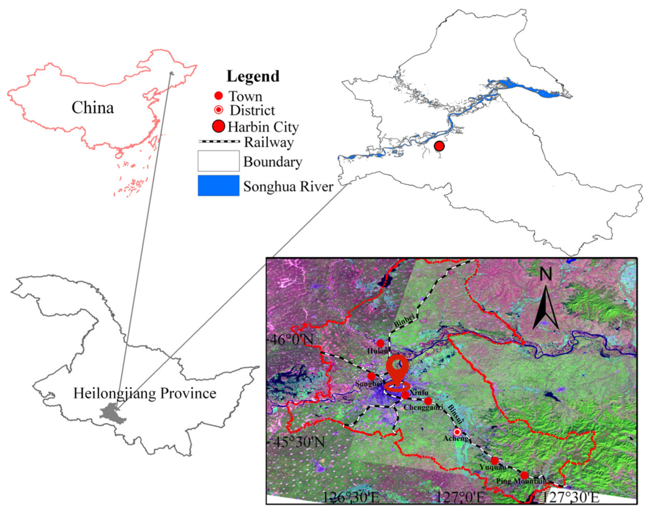
The geographic and climatic parameters of the observation site location mostly determine the aerosol properties. The high latitude city of Harbin (45.7165°N, 126.6318°E, as seen in
Figure 1), northeast China, is where the temperature and humidity profile lidar used in this investigation was placed. With a population of 9.395 million and a total area of 53,000 square kilometers, Harbin is a heavily populated metropolis. The lidar observation station was situated in the heart of the city, encircled by crowded business and residential districts. The observation period concentrated on February 2024. The InnoSlab laser had a repetition frequency of 2 kHz with emission wavelengths of 355 and 532 nm. The following signals were received using a telescope with a 300 mm aperture: temperature high and low order pure rotational Raman signals at 354 nm and 353 nm, respectively, the nitrogen vibrational Raman signals at 387 nm, the water vapor vibrational Raman signals at 407 nm, and the elastic scattering signals at 355 nm, 532P nm (parallel), and 532S nm (vertical). The transient recorder had two modes of operation: the analog mode detected powerful echo signals at low altitudes, while the photon counting mode detected weak echo signals at high altitudes. The analog mode and photon counting mode were spliced using a splicing technique. The data included a 7.5 m range resolution and a 5 min time resolution [
25].
Table 1 displays the system parameters of this lidar.
2.2. Signal Preprocessing
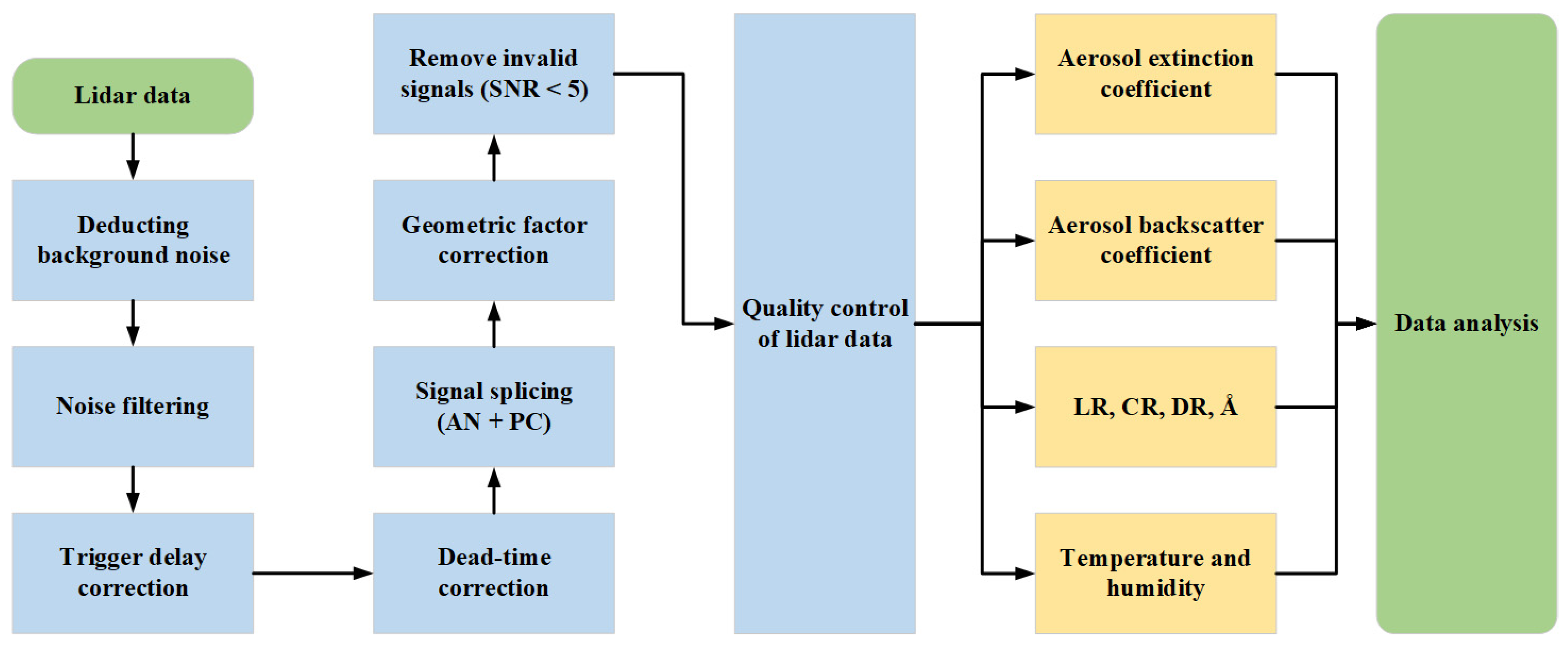
After system acquisition, the original signal must undergo preprocessing [
26], which includes background noise, atmospheric interference, electronic noise filtering [
27], photon counting signal dead zone correction, signal splicing, and geometric factor correction. The self-developed geometric factor correction algorithm in reference [
28] was used to correct and supplement the transition zone signal and blind zone signal of the Mie–Raman scattering channel, eliminating the distortion of near-ground blind zone signal and ensuring the spatial consistency of data within the urban canopy height range, in order to study the atmospheric environment near the ground. As described in references [
27,
28,
29], the data obtained from temperature and humidity profile lidar inversion were compared and validated with data from radiosondes and ground meteorological stations at the same location. The results show that the average temperature deviation was less than 2 K, and the relative humidity deviation was less than 5%. The correlation between visibility calculated from the aerosol extinction coefficient and visibility meter results was as high as 0.997. The effective detection time of the second-level data products of aerosols was mostly focused at night because the system’s vibration Raman scattering signal had a signal-to-noise ratio (SNR) that was significantly lower during the day than it was at night. To ensure data quality, we removed invalid data with the SNR < 5 from the dataset.
Figure 2 depicts the flow of data processing.
2.3. Methods
The aerosol extinction coefficient
αa and backscattering coefficient
βa can be inverted using the Raman method with no parameter assumptions [
30] as follows:
where
αm is the molecule extinction coefficient,
βm is the molecule backscattering coefficient,
λ0 is the emitting wavelength and
λR is the Raman wavelength,
k’s value is between 0 and 4,
N(
z) is the number density of nitrogen,
PR(
z) is the Raman echo signal,
P0(
z) is the elastic echo signal,
C is a calibration constant.
The laser lidar ratio (
LR), color ratio (
CR), depolarization ratio (
DR), and Ångström exponent (Å) at 355 nm and 532 nm wavelengths (
λ) can be expressed as follows [
22,
23]:
The number density of water vapor
can be obtained by the ratio of the vibrational Raman signals of water vapor
and nitrogen gas
[
28]:
The atmospheric temperature
T(
z) is inverted from the quotient of high- and low-order pure rotational Raman signals
Q(
z) [
25]:
where
a,
b, and
c are calibration coefficients.
2.4. HYSPLIT
The National Oceanic and Atmospheric Administration of the United States and the Australian Bureau of Meteorology collaborated to develop the professional model known as HYSPLIT (Hybrid Single-Particle Lagrangian Integrated Trajectory model,
https://www.ready.noaa.gov/HYSPLIT.php, accessed on 1 February 2025) [
31], which is widely used to calculate and analyze the transport and diffusion trajectories of atmospheric pollutants. The origins, transport, and diffusion mechanisms of aerosols were assessed in this work using the HYSPLIT backward trajectory analysis model. On a local to global scale, the HYSPLIT model replicates the diffusion and trajectory of materials that are carried and distributed through the atmosphere. The transport, diffusion, and deposition of pollutants and hazardous compounds in the atmosphere have all been described using it in a variety of simulations. The Global Data Assimilation System computed the backward trajectories of various heights in 36 h and recorded meteorological data every six hours.
3. Results
The monitoring of the temperature and humidity profile lidar in Harbin started in February 2024. Harbin, a heavily industrial city, has historically had significant levels of pollution emissions. Due to the requirement for urban heating and other coal emissions, this is particularly true during the frigid winter months. The Chinese New Year and Yuanxiao Festival took place during the observation period, and the city experiences additional pollution as a result of the massive celebrations. Three common pollution cases— severe, moderate, and mild pollution—were covered in this study. PM2.5(10) is defined as particulate matter with an aerodynamic diameter less than 2.5 (10) μm. Continuous monitoring data of pollution tracers, such as PM2.5 and PM10, were collected hourly from environmental monitoring sites within 3 km of one another.
3.1. Severely Polluted Case
First, we chose a typical case of severe haze pollution (Case 1), where the maximum value of PM
2.5(10) was near 600 (800) μg/m
3, and the average value was over 180 (200) μg/m
3. This case was observed from 8 February 2024, at 16:00 until 11 February 2024, at 8:00 (China Standard Time).
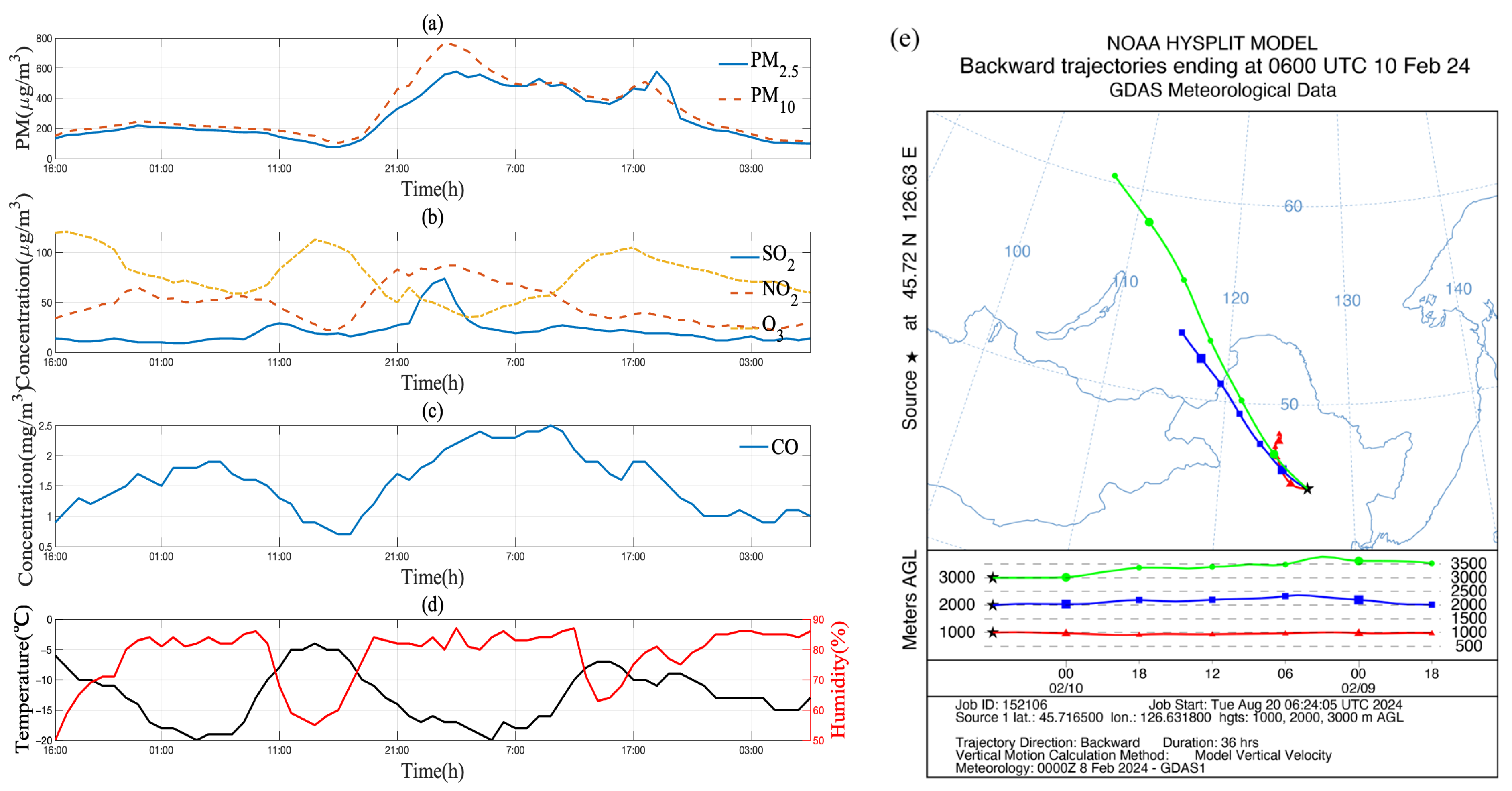
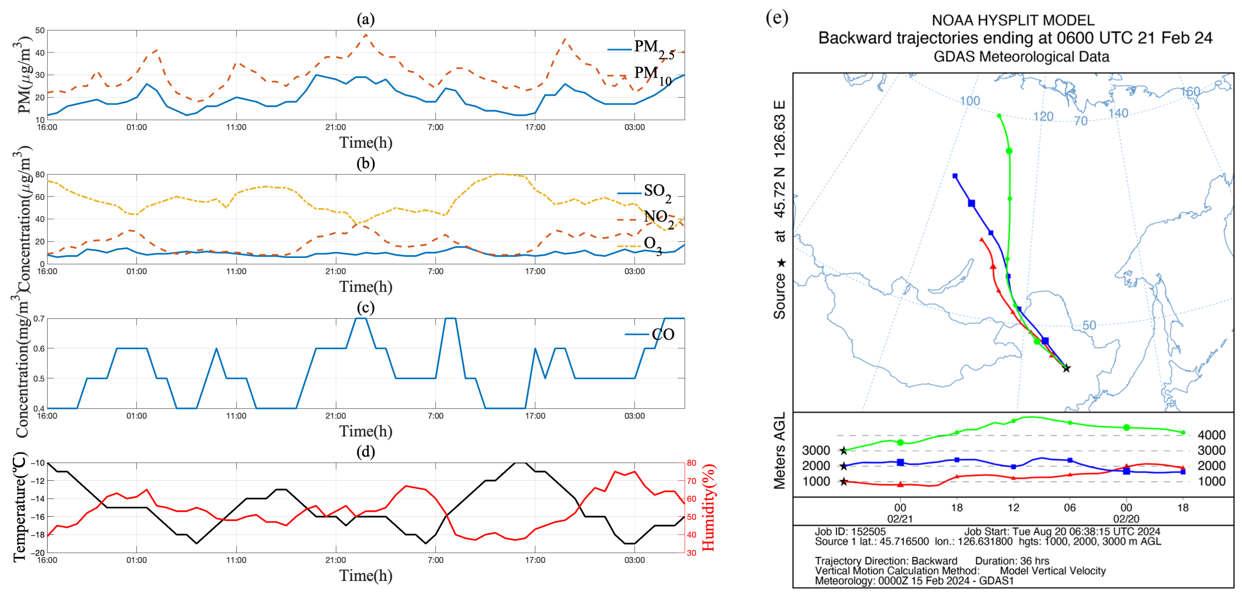
Figure 3 displays the environmental monitoring station’s data on ground environmental monitoring (from:
https://www.aqistudy.cn/, accessed on 1 February 2025). The early morning of 10 February saw the apex of the PM
2.5(10) pollution distribution under extreme pollution circumstances, along with significant SO
2, NO
2, and CO generation. This is due to the fact that China is currently celebrating the Chinese New Year. Many residents in the neighborhoods surrounding the city lit firecrackers and fireworks to commemorate this great celebration, which caused the production of a lot of combustion products and polluting gas molecules in the urban canopy layer (UCL) and urban boundary layer (UBL). The trajectories of air masses at various heights over the city during the observation period originated from the northwest, drifting from sparsely populated Siberia to above the observation point, as shown in
Figure 3e. The transmission between each layer was smooth and free of mixing phenomena. They primarily went along particular routes at their various elevations, which might cause pollutants to build up at particular elevations.
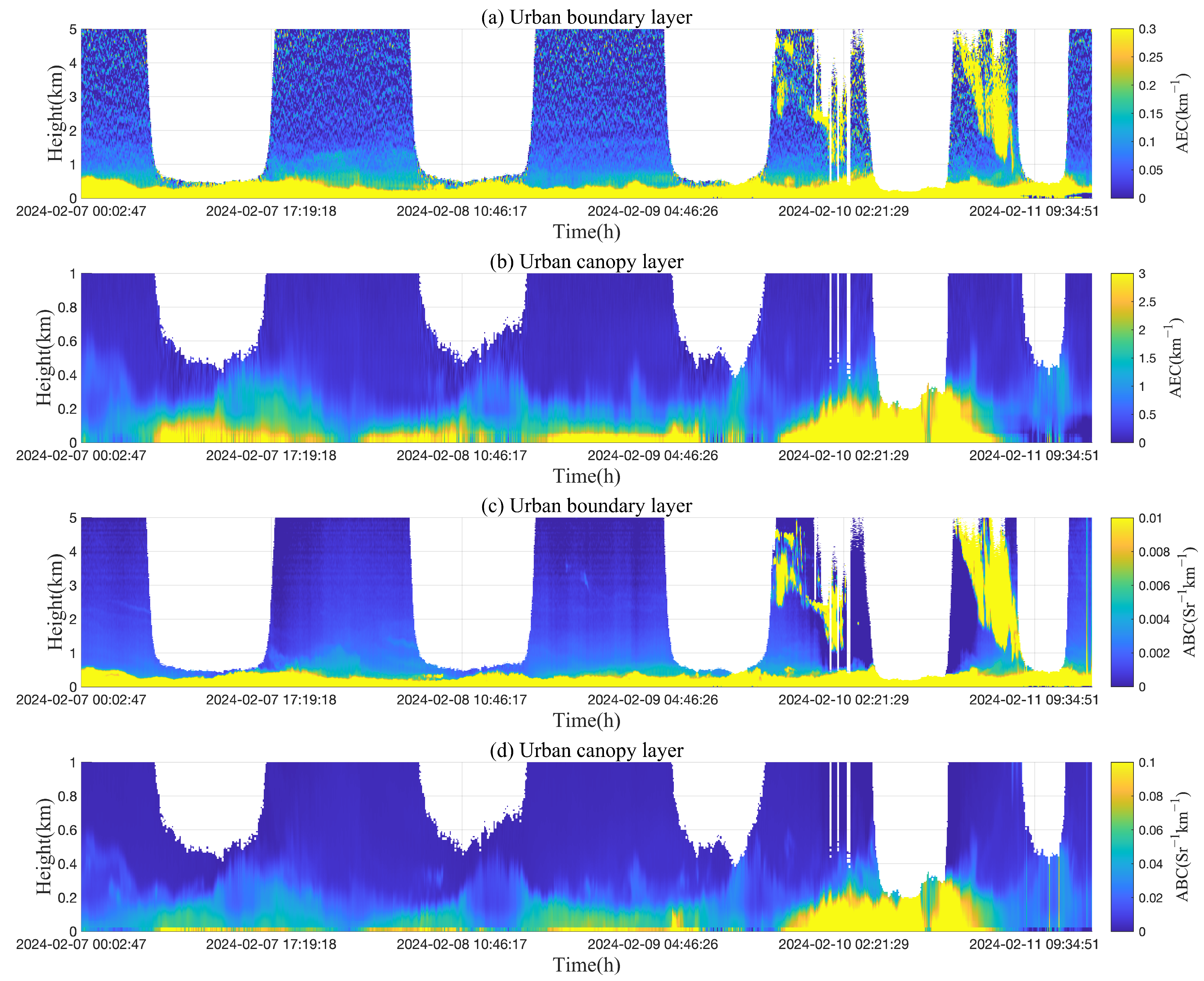
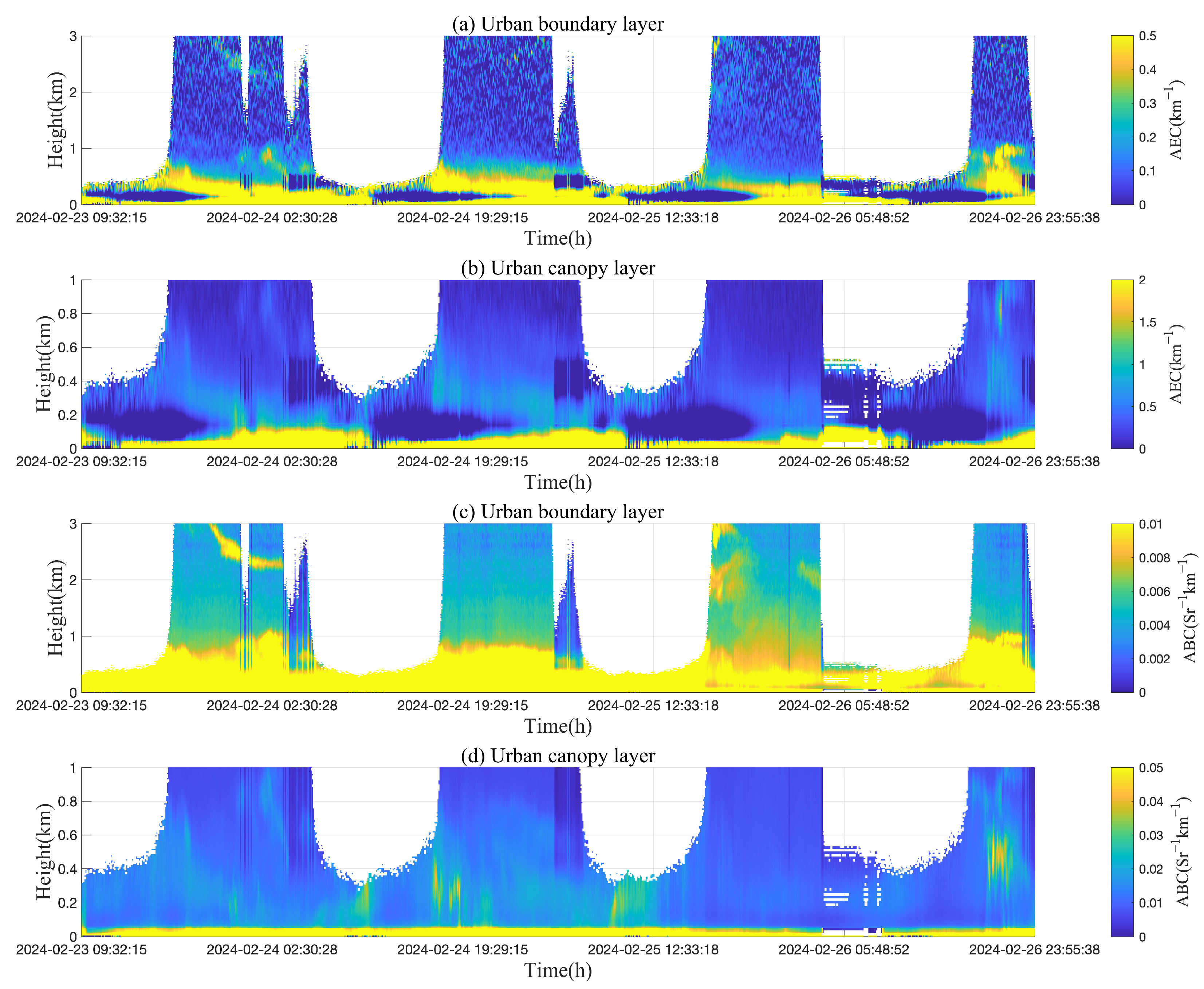
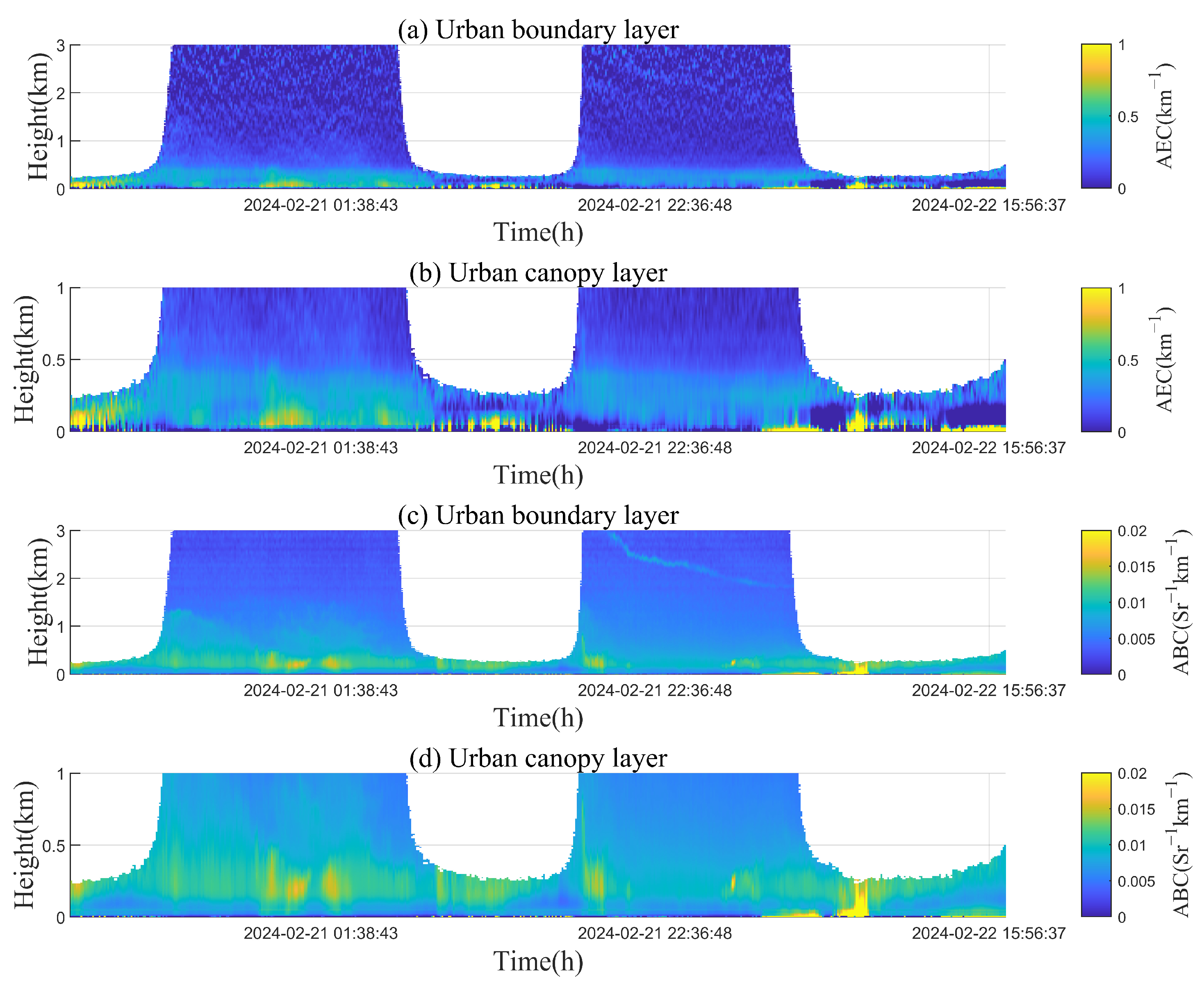
Figure 4 displays the temperature and humidity profiles’ lidar measurements of the first-level aerosol optical parameters (AEC and ABC) of Case 1. The reason for the blank data in the figure is due to the insufficient signal-to-noise ratio of the Raman scattering signal. Specifically, the strong background radiation in the daytime sky significantly interferes with the detection of Raman scattering signals, resulting in a significant decrease in signal-to-noise ratio. This interference makes the originally weak Raman scattering signal tail more short-lived, thereby masking a large amount of valuable information with noise. Nevertheless, nighttime observation data can still capture the core period of urban air pollution, which is effective for our current research. The high-altitude air mass carried some pollutants during the period from 9 February to 11 February, as depicted in
Figure 4a,c. These pollutants were transported to the observation point twice in a row by the high-altitude air mass, where they gradually settled at a height of 1 km, infiltrating the urban boundary layer, and then gradually spreading and becoming eliminated in the early morning of 10 February and during the day on 11 February. On the evening of 9 February, as midnight drew near, more and more pollutants from firecrackers and fireworks were seen in the Harbin region, as seen in
Figure 4b,d. AEC and ABC values rapidly increased as a result of the particles produced by these burning operations rapidly spreading and congregating throughout the metropolis. It is evident from the pollutants’ diffusion height and time dimensions that the pollutants produced by human activity had not risen much to higher latitudes and were primarily concentrated in the underlying surface area. In the urban canopy layer within 400 m, on 10 February, the AEC of severe haze particles was 2.77–6.21 km
−1, and the ABC was 0.08–0.15 Sr
−1 km
−1. The wind speed near the ground was below the critical threshold for pollutant diffusion [
32], resulting in PM
2.5 continuously accumulating in the near-surface layer. The HYSPLIT trajectory showed that the movement speed of the air mass matched the low wind speed, which prolonged the local retention time of pollutants from fireworks (peak duration > 12 h).
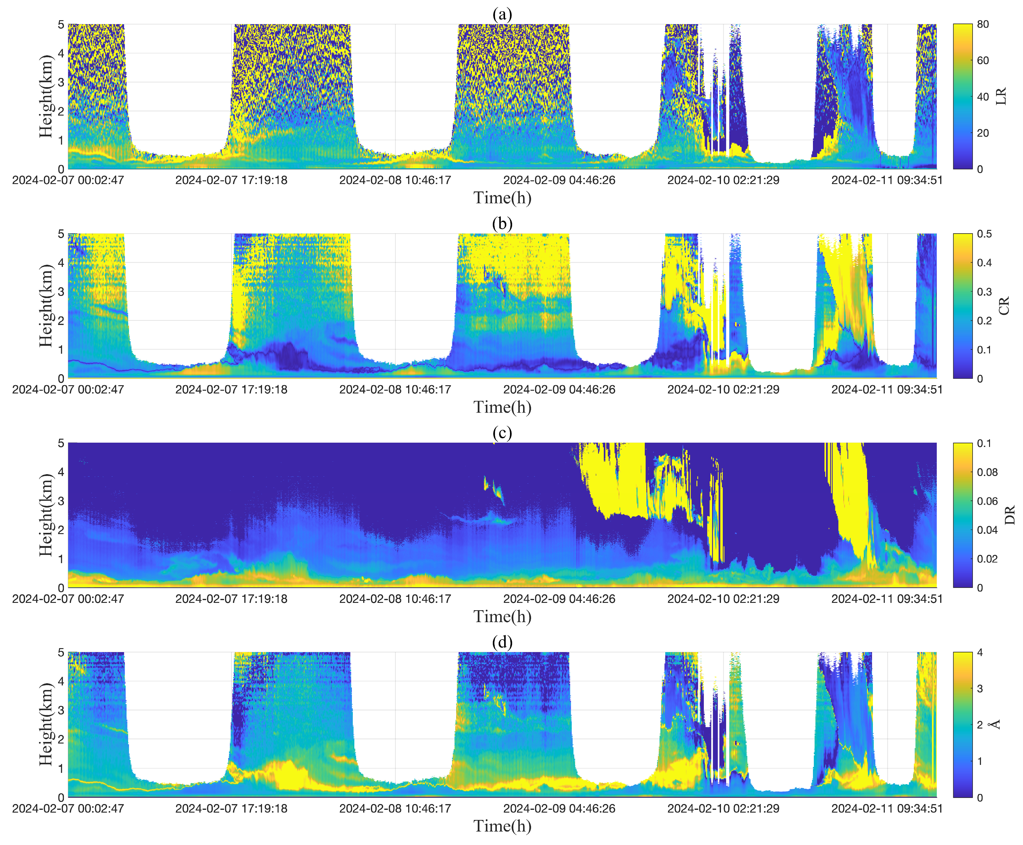
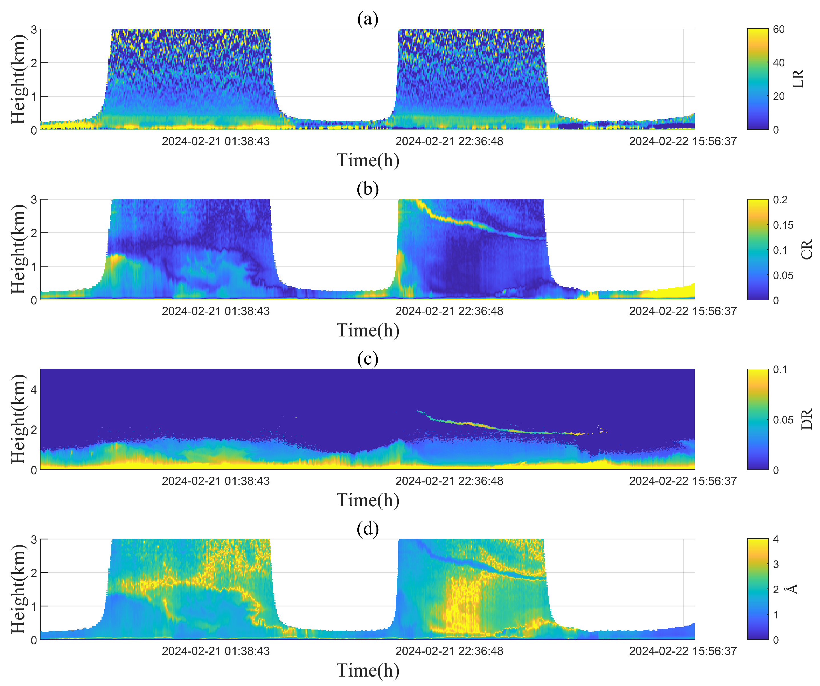
Figure 5 displays the second-level aerosol optical characteristics (LR, CR, DR, and Å) that are lidar inverted.
Figure 5a shows that the LR had a wide range of temporal and spatial fluctuation, ranging from 22 to 85 Sr, as a result of the aerosol particle size and microphysical characteristics changing with height. The size of the LR value depends on the particle size and refractive index of the aerosol. The decrease in its value may be due to the shape effect of aerosol particles and relatively low absorption efficiency. The increase in its value was related to the simultaneous increase in AEC and ABC caused by pollution, but the backscattering amplification was faster. The DR in
Figure 5c demonstrated that a significant number of non-spherical particles appeared on two nights on the day before the occurrence of severe pollution (9 February), gradually diffusing and settling from an altitude of 3–5 km or more, influencing the particle distribution in the urban boundary layer and urban canopy layer. These high-altitude particles originated from Siberia and influenced the diffusion process of combustion particles created by fireworks and firecrackers, as shown by the backward trajectory in
Figure 3e. This causes corresponding changes in CR and Å related to particle size in
Figure 5b,d, specifically one decreased and one increased. The CR rose from less than 0.1 to approximately 0.35, starting in the early hours of 10 February, suggesting that the type of pollution had shifted to coal smoke particulate matter, which was comparable to the hypothesized byproducts of firecracker and firework combustion. This indicated that human combustion activities were the primary cause of this pollution. There was a strong association between the average radius of aerosol particles and the size of the Å value. The Å value approaches 0 when the radius of the aerosol particles is very small in relation to the incident laser’s wavelength, and it declines as the particle size increases. The Å value gradually decreased from high during the night of 9 February to the early morning of 10 February, indicating that coarse particles replaced fine particles as the main component of pollutants. This change in particle radius was caused by combustion products.
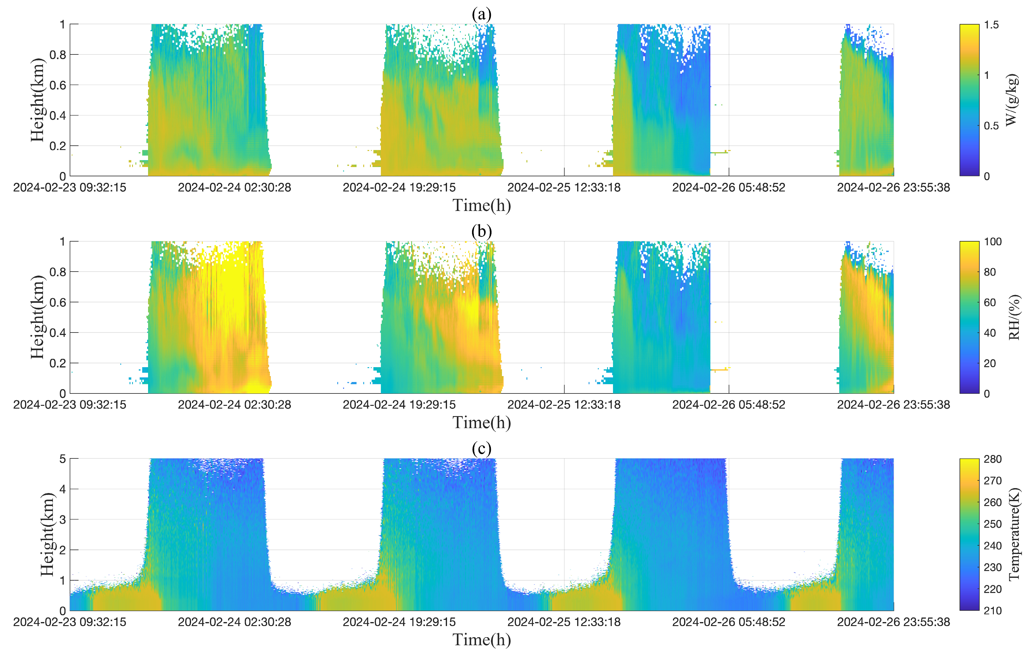
Figure 6 displays the detected temperature and humidity profiles, and the environmental monitoring station’s data were in agreement with the temperature and humidity variations near the ground throughout the day. The temperature and humidity correlations between the two instruments were 0.93 and 0.89, respectively. Due to an inadequate signal-to-noise ratio, the vibration Raman scattering signal was missing a significant quantity of daytime data on the day of the extreme pollution. The water vapor content in the urban canopy layer climbed steadily, starting on the night of 9 February, and peaked at 5 am on 10 February, according to detection data collected within 100 m of the ground. Harbin typically experienced nighttime temperatures below 265 K. By suppressing the flow of the atmosphere over the city, limiting the violent movement of turbulence over the city, and limiting the speed at which pollutants diffuse, the low temperature and high humidity altered the microphysical characteristics of aerosols. This included causing aerosol hygroscopic growth, increasing the production of condensation nuclei, and worsening pollution. The contaminants in the urban canopy layer started to slowly disappear as atmospheric turbulence increased when the sun rose on February 10th and the city temperature rose.
3.2. Moderately Polluted Case
The highest value in this case exceeded 250 (300) μg/m
3, and the average PM
2.5(10) was higher than 70 (100) μg/m
3. This case was observed between 23 February 2024, at 16:00 and 26 February 2024, at 8:00 (China Standard Time).
Figure 7 displays the ground environmental monitoring data collected from the environmental monitoring station. On the evening of 24 February, which was also the night of the Yuanxiao Festival, PM
2.5(10) reached its peak. There was no widespread or persistent pollution, although some residents lit candles or fireworks to commemorate the event and offer prayers. The pollutants progressively vanished during the afternoon of 25 February. This was corroborated by the combustion products CO and NO
2. The air pollution above the observation point would be influenced by emissions from nearby cities, such as traffic, industrial, or residential emissions, as
Figure 7e shows that the particulate matter air mass above the city originates from nearby cities. When particles of various heights arrived at the observation site, their routes diverged and there was no mutual interference, notwithstanding the initial cross-transmission. Among these, the air mass at a height of 3 km displayed local cyclic transmission, which might be brought on by regional weather and geographic factors. The other two air masses might carry pollution to the surrounding areas, as seen by their very short transmission pathways.
Figure 8 displays the temperature and humidity profile lidar’s first-level aerosol optical characteristics of Case 2. Fluorescence effects had affected certain readings close to the ground. In order to deliver higher-quality data, we will concentrate on resolving this issue in further work. However, the majority of the detection data was valid, and these incorrect data only made up a minor percentage. The monitoring data showed that on the day of the Yuanxiao Festival, the AEC near the ground fluctuated at 2.13 km
−1, while the transmission of aerosol particles was comparatively steady. Although the pollution level was not high overall, it did grow in the early morning hours on 25 February. This did not significantly affect local productivity. The emission of exhaust gases from people’s heating and driving systems, as well as the deposition of air aerosols on the ground, might be the cause of the generally high aerosol extinction coefficient near the ground during the observation period.
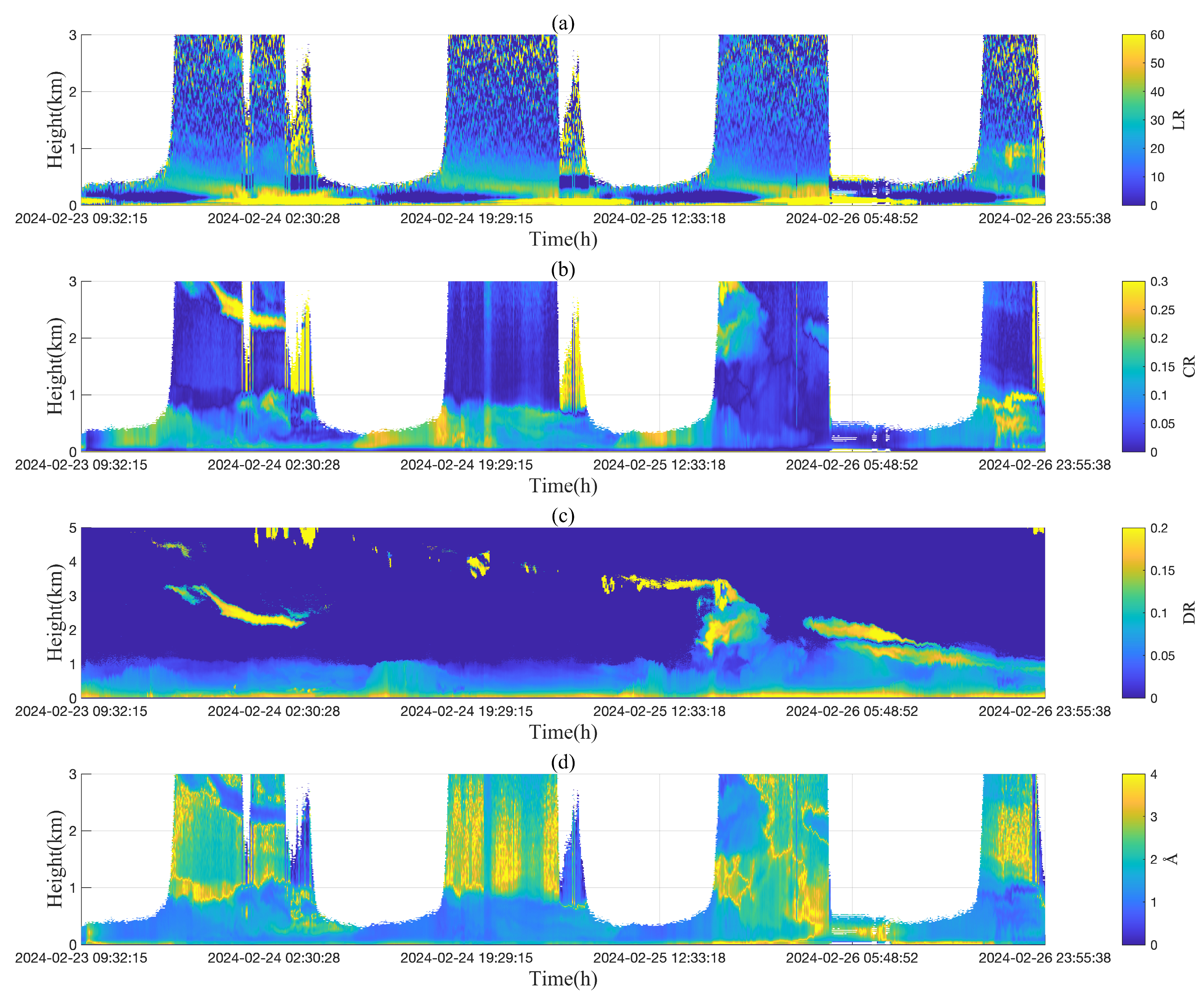
Figure 9 displays the observation data for the aerosol optical properties at the second level.
Figure 9a shows that the LR changed between 25 and 45 Sr during the small pollution period and between 48 and 66 Sr throughout the pollution incidence period. The LR, on the other hand, exhibited a periodic trend, suggesting that the atmospheric dynamics over the city held steady throughout the observation period, and there was some regularity in the convergence and diffusion of pollutants. The range of CR variation, which was linearly correlated with the aerosol particle size, was 0.12–0.23 from the evening of the 24th to the daytime of the 25th and progressively declined; this showed that the particles were gradually diffusing and eliminating. The DR variation over the same time period showed a change in the sphericity of the combustion-produced aerosol particles. Dust with a DR value of roughly 0.3 started to appear 3–3.8 km above the city on the 25th. It slowly filtered into the urban boundary layer and altered its height, which meant this dust was typical of Asia [
33]. Relatively little variation in the Å value, which was inversely related to the particle size, suggested that the duration and impact of the entire pollution process were minimal and that the particle size did not change significantly over the course of the pollution period. The strong winds in the middle layer accelerated the vertical mixing of sand and dust particles [
34], causing the sand and dust to rapidly sink to the boundary layer. The wind speed near the ground was close to the cleaning threshold, which made the emission pollution of the Yuanxiao Festival drop rapidly, reflecting the rapid removal effect of wind speed on local sources.
Figure 10 displays the temperature and humidity profiles that were gathered. The vibration Raman scattering signal’s signal-to-noise ratio decreased throughout the day due to the strong sky background radiation, and the water vapor inversion results during the day were absent. The temperature and humidity inversion data showed no interference from Mie-scattering, suggesting that the system’s optical architecture was capable of successfully suppressing stray light interference. It was evident from the relative humidity distribution on the night of the 24th that the water vapor content was stratified above the urban canopy layer and progressively rose over time. The temperature in this instance rose by roughly 5–7 K throughout the course of the night of the 24th in comparison to Case 1, which would have comparatively accelerated air movement and increased the turbulent motion of the underlying mat, both of which were favorable for the diffusion of pollutants. During the observation period, there was no discernible inversion layer, and the impacts of thermodynamics and aerodynamics were minimal.
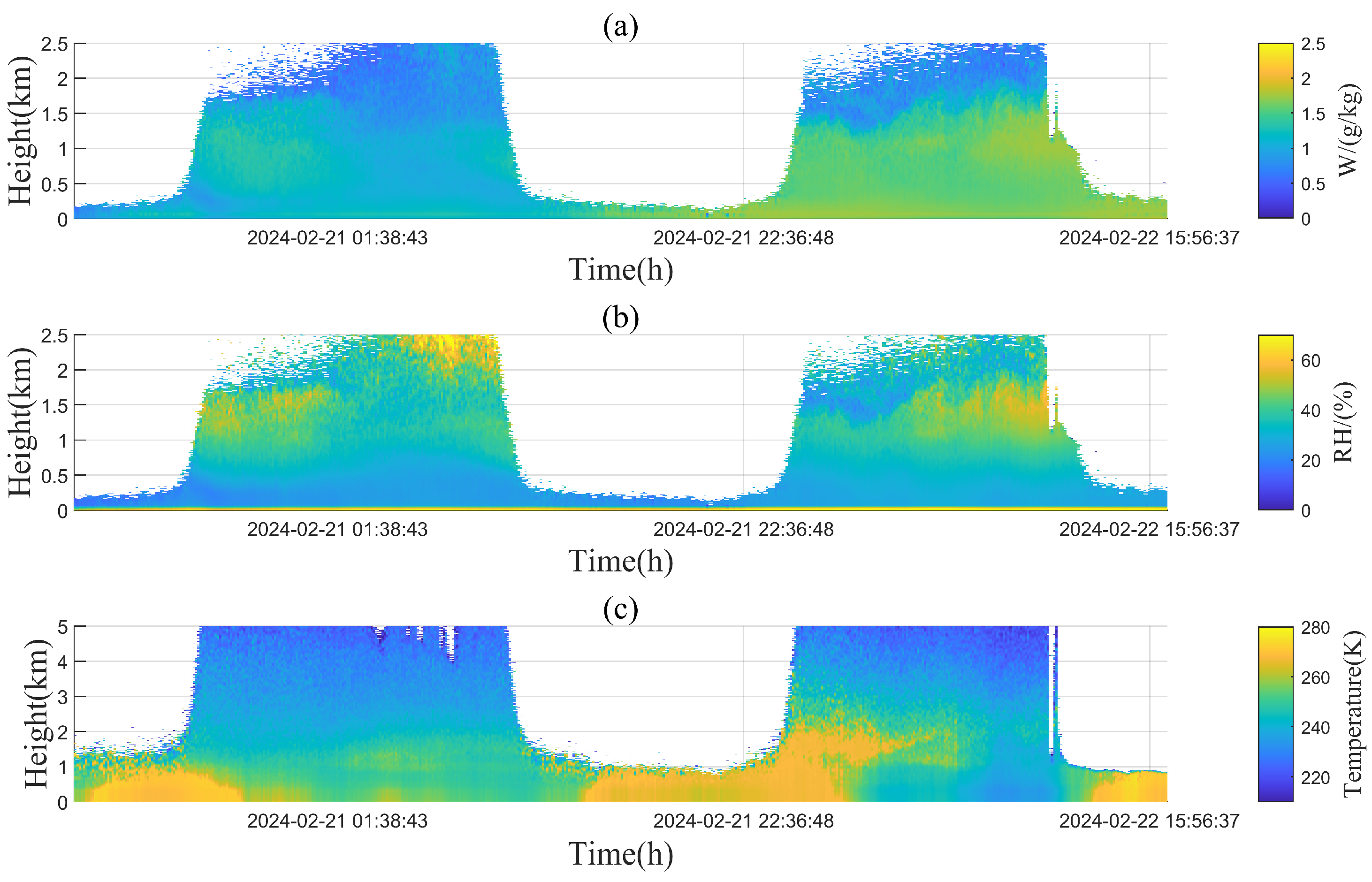
3.3. Mildly Polluted Case
Mild pollution incidents were observed between 19 February 2024, at 16:00 and 22 February 2024, at 8:00 (China Standard Time).
Figure 11 displays the ground pollution data that was acquired from the environmental monitoring station. Mild pollution as indicated by an average PM
2.5(10) of less than 30 (50) μg/m
3. The observation period fell throughout working days, and human activities, with vehicle exhaust fumes and dust from building sites and roads during commuting being the main causes of urban pollution. The air mass over the city originates in Siberia, Russia, traveling via the Greater Khingan Mountains forest area and Inner Mongolia grassland, and being rather gently transmitted to the airspace over Harbin, according to the backward trajectory map in
Figure 11e. The transmission path and velocity of air masses might be significantly impacted by the Greater Khingan Range region, which is a significant geographical and climatic barrier. Mountains have the power to alter wind speed and direction, which can cause air masses to rise or fall and alter their transmission patterns. A mixing of air masses from several sources in the lower atmosphere might be indicated by the crossing of low air masses.
Figure 12 displays the aerosol optical properties at the first level of Case 3. The air environment within the UCL and UBL was comparatively clean, and the ranges of AEC and ABC were 0.1–0.46 km
−1 and 0.01–0.017 Sr
−1 km
−1, respectively. There was no notable pollution outbreak throughout the observation period. The ABC distribution indicated that the primary source of pollution in the Harbin area was the exhaust gas produced by thermal heating and that the location was comparatively cool at night. Additionally, this resulted in a higher aerosol concentration at night as opposed to during the day, which raised the ABC value.
Figure 13 displays the second-level aerosol optical characteristics as determined by the lidar. Because aerosol particle size and microphysical characteristics change with height, the LR varied about 35 Sr and decreased as height increased. Lower aerosol concentration and lower aerosol absorption efficiency are associated with an average LR value above 200 m, which here was typically less than 40 Sr [
35]. Since CR fluctuated by around 0.1 and DR fluctuated steadily, non-spherical particles above the city were unaffected by outside pollution sources. There might be more fine particles in the air, as shown by the lower Å value. The status of ice crystals and water vapor within thin clouds at a height of 2–3 km on the night of the 21st was continuously changing, and its phase change process merited further thorough investigation. The DR of these clouds was between 0.035 and 0.082. The wind speed near the ground was higher than the diffusion threshold, which significantly improved the diffusion efficiency of fine particulate matter emitted from traffic. The combined effect of wind speed on the transmission path of air masses and terrain obstruction in the Greater Khingan Range reduced external pollution input, verifying the representativeness of clean air masses [
36].
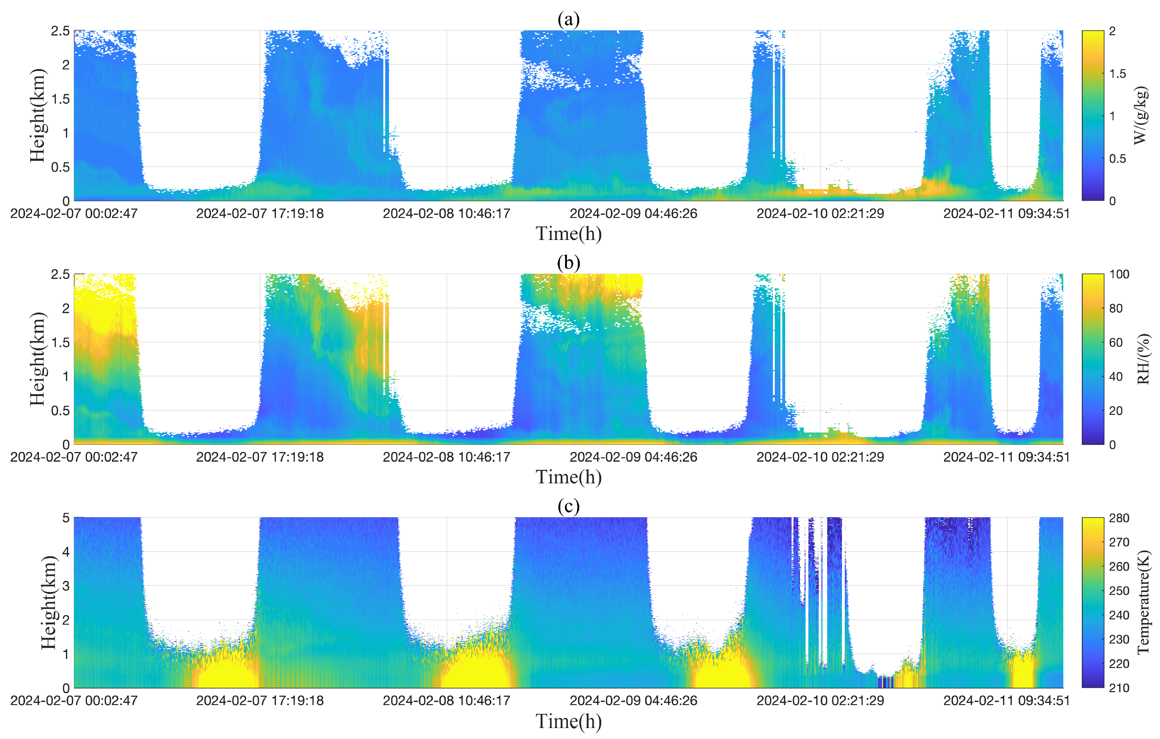
Figure 14 displays the profiles of temperature and humidity. The amount of water vapor over the city steadily rose as the observation period went on. Without the occurrence of extreme weather circumstances such as abrupt chilling and heating, the temperature variation throughout the day also complied with the rules of aerodynamics. Significant changes in the CR and Å values in
Figure 13 were caused by a temperature inversion layer that persisted for two hours at a distance of 1 km in the early morning of the 21st. This layer altered the atmospheric structure and had an impact on turbulent motion. A temperature inversion layer formed at 2 km on the night of the 21st, while the water vapor was evenly distributed, which significantly affected aerosol transport and alterations.
4. Discussion
The thorough examination of the aforementioned data showed in Case 1, despite the possibility of some contaminants brought by Siberian air masses momentarily lowering city air quality, efficient governance actions had significantly improved air quality. The fact that contaminants with high concentrations only spread over a single day serves as proof of this. Below 1 km, the AEC and ABC were comparatively large, suggesting the existence of a thick concentration of the aerosol layer in this region. The characteristics of dust particles at this height were also rather diverse and complex, as can be seen from the four typical values of the secondary parameters. This suggested that the particle properties in this height range were constantly changing. According to Franke et al. [
37], fine particles (urban haze with strong light absorption) have a greater LR value than coarse particles. Consequently, relatively coarse particles make up the majority of pollutants in this highly polluted air environment. While a low-temperature environment could alter the thermal motion state of molecules in the atmosphere, suppress turbulent activity, indirectly affect laser propagation and scattering, and increase CR values, a high-humidity atmospheric environment on the day of pollution may cause aerosol particles to absorb moisture and increase, changing their scattering characteristics. It might be inferred from the trend of concurrent increases in ABC and CR that the combustion products changed the optical and microphysical characteristics of the aerosols, including increasing particle size and improving scattering ability. In addition, aerosols significantly affect the atmospheric temperature profile by absorbing and scattering solar radiation (direct effects) and acting as cloud condensation nuclei to alter cloud albedo and lifetime (indirect effects). High-concentration aerosols form the “umbrella effect” and “dome effect” by absorbing shortwave radiation (such as black charcoal aerosols) and scattering longwave radiation (such as sulfate aerosols). This process was similar to the observation results in Beijing and other places [
38,
39], that is, aerosol radiative forcing will cause a decrease in the turbulent kinetic energy index of the boundary layer, and the height of the boundary layer will be compressed.
It was possible to deduce from Case 2 that some foreign contaminants were progressively carried over the observation point by the combined impact of westerly, northwesterly, and southwesterly winds. The DR distribution indicated that certain non-spherical particles were carried by these air masses. This was because the air mass’s route was communicated locally and passed over several heavily industrialized cities. Poor air quality in the city has always been caused by a small amount of pollution in the urban canopy layer in low-altitude places, as could be observed by the distribution of PM2.5(10), AEC, and ABC. Dust and anthropogenic particles were the major components of particulate components under moderate pollution circumstances. Furthermore, the majority of these secondary data did not exhibit appreciable distortion, suggesting that there were no notable alterations in the optical and microphysical characteristics of aerosol particles throughout the observation period. The steady temperature variations further demonstrated that there was no significant change in the city’s atmospheric properties over this time.
The data analysis from Case 3 led to the conclusion that the LR rapidly reduced with increasing altitude within the UCL below 500 m. This was because the nighttime inversion in the UBL at low altitudes reduced the vertical movement of the atmosphere, which inhibited the diffusion of pollutants released by human activities like driving and burning fossil fuels. Significant variations in the vertical distribution of aerosols were caused by the buildup of pollutants in the lower UBL, and the extinction coefficient of aerosols rapidly dropped within the boundary layer [
40,
41]. The variation in LR between various height ranges was comparatively modest in the UBL above 500 m because of the low concentration of aerosols, their tiny size, and their uniform vertical distribution. Particle size was affected by a temperature inversion layer that was present on the early morning of the 21st. The presence of the temperature inversion layer would result in a drop in particle size as well as a change in the form and structure of the particles based on the decrease in CR and the increase in Å value. Dust particles (nonspherical, high depolarization ratio) have strong absorption of longwave radiation and can heat the middle atmosphere, forming an abnormal temperature gradient of “warm-up and cold-down”, further suppressing convection. Coal smoke and black carbon aerosols (highly absorbent) significantly heat the atmosphere from near the ground to 2.5 km through shortwave absorption, leading to a reduction in the temperature difference between day and night at high altitudes. This phenomenon has been recorded in the transmission pathways of sand and dust in East Asia and urban pollution cases, which is similar to the simulation results of the aerosol radiation boundary layer interaction model in the literature [
42,
43]. Based on HYSPLIT trajectory analysis, the dust carried by Siberian air masses mixed with local coal gas aerosols may form a persistent “pollution dome” through radiation heating of the middle atmosphere.
5. Conclusions
The first urban atmospheric environment monitoring activity was carried out in Harbin, a high-latitude region of China, and was based on the temperature and humidity profile lidar. The environmental monitoring station provided continuous monitoring ground data, and the HYSPLIT model was used to plot the air mass’s source route. The development of atmospheric environment monitoring activities in the urban canopy layer and urban boundary layer was made possible by the continuous collection of aerosol primary and secondary optical parameters, as well as temperature and humidity data, using the temperature and humidity profile lidar. The observation period of this study is concentrated in winter, mainly reflecting the pollution characteristics of Harbin during the cold season. Due to significant seasonal differences in the atmospheric environment of high-latitude cities (such as spring dust storms and summer photochemical pollution), it is necessary to extend the observation period (such as year-round coverage) and combine historical data to further verify the universality of the conclusions in the future.
Under various atmospheric pollution circumstances, the distribution of the second-level aerosol optical parameters (LR, CR, DR, and Å) obtained by temperature and humidity profile lidar varied. The properties of LR changes could be influenced by aerosol type, composition, concentration, and form. The size of CR could be influenced by various laser emission wavelengths, particle properties, etc. One important aspect influencing DR was the shape change of non-spherical particles. Environmental factors like temperature and humidity had a significant impact on the diffusion and aggregation of aerosols, particularly when temperature inversion and high humidity were present. Å was a measure of how sensitive particle size was to wavelength. In the severely polluted case, the combustion products could alter the distribution of particle concentration, size, and composition, high-humidity and low-temperature environments could cause aerosol particles to absorb moisture and grow, altering turbulent structures and the thermodynamic motion of particles and extending the time it took for pollutants to diffuse. Compared with low-latitude cities such as Shanghai and Guangzhou, the synergistic effect of winter low temperature and high humidity in Harbin significantly exacerbates the growth of aerosol moisture absorption. Under moderate pollution weather conditions, a continuously changing atmospheric environment could lead to a certain pattern of pollutant changes. The external sand and dust transported and infiltrated above the observation point could alter the structure of the UBL and affect particle properties. Increased airflow velocity sped up the diffusion of pollutants, and particulate matter carried by aerosol air masses from nearby places might be the primary source of persistent pollution close to the ground in urban areas. After mixing dust air masses from Siberia with fine particulate matter emitted from local coal combustion, they exhibit unique characteristics of “high LR and low DR”, which are significantly different from pure dust (low LR, high DR) or pure urban aerosols (high LR, high DR). The stability of atmospheric changes above cities could be further demonstrated by the steady temperature change process. Overall changes in aerosol optical parameters were negligible in clear weather, and low humidity conditions made it difficult to modify the microphysical characteristics of aerosols. Polluting particles were rarely present in air masses that moved through forest fields and grasslands. The size and diffusion of particles might be affected by temperature inversion. In contrast to the other two scenarios, the aerosols’ primary and secondary optical parameter changes were comparatively steady.
The LR, CR, DR, and Å characteristics derived from aerosol detection are complicated and challenging to measure, according to our research. In the future, long-term measurements of parameters like LR, CR, DR, and Å will still require the employment of temperature and humidity profile lidar and other sensors. More research is needed to determine how they relate to other optical factors or atmospheric conditions.
Author Contributions
Methodology, B.Z., T.Z. and W.L.; validation, B.Z., G.F. and X.J.; writing-original draft preparation, B.Z. All authors have read and agreed to the published version of the manuscript.
Funding
This research has been supported by the National Key R&D Program of China (2022YFC3700400, 2022YFC3704000). This achievement has received funding from the Hefei Comprehensive National Science Center.
Data Availability Statement
The datasets used and analyzed during the current study are available from the corresponding author upon reasonable request.
Acknowledgments
We appreciate Ruxia Ma and Zhizi Zhang for checking and improving the English spelling of this article.
Conflicts of Interest
The authors declare no conflicts of interest.
References
- Radlach, M.; Behrendt, A.; Wulfmeyer, V. Scanning rotational Raman lidar at 355 nm for the measurement of tropospheric temperature fields. Atmos. Chem. Phys. 2008, 8, 159–169. [Google Scholar] [CrossRef]
- Hicks-Jalali, S.; Sica, R.J.; Martucci, G.; Barras, E.M.; Voirin, J.; Haefele, A. A Raman lidar tropospheric water vapour climatology and height-resolved trend analysis over Payerne, Switzerland. Atmos. Chem. Phys. 2020, 20, 9619–9640. [Google Scholar] [CrossRef]
- Wang, W.; Huang, J.; Zhou, T.; Bi, J.; Lin, L.; Chen, Y.; Huang, Z.; Su, J. Estimation of radiative effect of a heavy dust storm over northwest China using Fu–Liou model and ground measurements. J. Quant. Spectrosc. Radiat. Transf. 2013, 122, 114–126. [Google Scholar] [CrossRef]
- Huang, J.; Wang, T.; Wang, W.; Li, Z.; Yan, H. Climate effects of dust aerosols over East Asian arid and semiarid regions. J. Geophys. Res. Atmos. 2014, 119, 11398–11416. [Google Scholar] [CrossRef]
- Huang, J.; Minnis, P.; Lin, B.; Yi, Y.; Fan, T.F.; Sun-Mack, S.; Ayers, J.K. Determination of ice water path in ice-over-water cloud systems using combined MODIS and AMSR-E measurements. Geophys. Res. Lett. 2006, 33, 1522–1534. [Google Scholar] [CrossRef]
- Pan, Z.; Gong, W.; Mao, F.; Li, J.; Wang, W.; Li, C.; Min, Q. Macrophysical and optical properties of clouds over East Asia measured by CALIPSO. J. Geophys. Res. Atmos. 2015, 120, 11653–11668. [Google Scholar] [CrossRef]
- Yan, H.; Wang, T. Ten Years of Aerosol Effects on Single-Layer Overcast Clouds over the US Southern Great Plains and the China Loess Plateau. Adv. Meteorol. 2020, 2020, 6719160. [Google Scholar] [CrossRef]
- Sicard, M.; Rocadenbosch, F.; Reba, M.N.M.; Comerón, A.; Tomás, S.; García-Vízcaino, D.; Batet, O.; Barrios, R.; Kumar, D.; Baldasano, J.M. Seasonal variability of aerosol optical properties observed by means of a Raman lidar at an EARLINET site over Northeastern Spain. Atmos. Chem. Phys. 2011, 11, 175–190. [Google Scholar] [CrossRef]
- He, Q.S.; Li, C.C.; Mao, J.T.; Lau, A.K.H.; Li, P.R. A study on the aerosol extinction-to-backscatter ratio with combination of micro-pulse LIDAR and MODIS over Hong Kong. Atmos. Chem. Phys. 2006, 6, 3243–3256. [Google Scholar] [CrossRef]
- Chen, W.N.; Chang, S.Y.; Chou, C.C.K.; Fang, G.C. Total scatter-to-backscatter ratio of aerosol derived from aerosol size distribution measurement. Int. J. Environ. Pollut. 2009, 37, 45–54. [Google Scholar] [CrossRef]
- Fan, G.; Zhang, B.; Zhang, T.; Fu, Y.; Pei, C.; Lou, S.; Li, X.; Chen, Z.; Liu, W. Accuracy Evaluation of Differential Absorption Lidar for Ozone Detection and Intercomparisons with Other Instruments. Remote Sens. 2024, 16, 2369. [Google Scholar] [CrossRef]
- Fernald, F.G. Analysis of atmospheric lidar observations: Some comments. Appl. Opt. 1984, 23, 652–653. [Google Scholar] [CrossRef]
- Gong, W.; Liu, B.; Ma, Y.; Zhang, M. Mie LIDAR Observations of Tropospheric Aerosol over Wuhan. Atmosphere 2015, 6, 1129–1140. [Google Scholar] [CrossRef]
- Fan, S.; Liu, C.; Xie, Z.; Dong, Y.; Hu, Q.; Fan, G.; Chen, Z.; Zhang, T.; Duan, J.; Zhang, P.; et al. Scanning vertical distributions of typical aerosols along the Yangtze River using elastic lidar. Sci. Total. Environ. 2018, 628–629, 631–641. [Google Scholar] [CrossRef]
- Ma, X.; Wang, C.; Han, G.; Ma, Y.; Li, S.; Gong, W.; Chen, J. Regional Atmospheric Aerosol Pollution Detection Based on LiDAR Remote Sensing. Remote Sens. 2019, 11, 2339. [Google Scholar] [CrossRef]
- Lv, L.; Xiang, Y.; Zhang, T.; Chai, W.; Liu, W. Comprehensive study of regional haze in the North China Plain with synergistic measurement from multiple mobile vehicle-based lidars and a lidar network. Sci. Total Environ. 2020, 721, 137773. [Google Scholar] [CrossRef]
- Mishchenko, M.I.; Cairns, B.; Hansen, J.E.; Travis, L.D.; Burg, R.; Kaufman, Y.J.; Martins, J.V.; Shettle, E.P. Monitoring of aerosol forcing of climate from space: Analysis of measurement requirements. J. Quant. Spectrosc. Radiat. Transf. 2004, 88, 149–161. [Google Scholar] [CrossRef]
- Zhao, H.; Mao, J.; Zhou, C.; Gong, X. A method of determining multi-wavelength lidar ratios combining aerodynamic particle sizer spectrometer and sun-photometer. J. Quant. Spectrosc. Radiat. Transf. 2018, 217, 224–228. [Google Scholar] [CrossRef]
- Liu, Z.; Sugimoto, N.; Murayama, T. Extinction-to-backscatter ratio of Asian dust observed with high-spectral-resolution lidar and Raman lidar. Appl. Opt. 2002, 41, 2760–2767. [Google Scholar] [CrossRef]
- Bréon, F.-M. Aerosol extinction-to-backscatter ratio derived from passive satellite measurements. Atmos. Chem. Phys. 2013, 13, 8947–8954. [Google Scholar] [CrossRef]
- Ansmann, A.; Riebesell, M.; Wandinger, U.; Weitkamp, C.; Voss, E.; Lahmann, W.; Michaelis, W. Combined raman elastic-backscatter LIDAR for vertical profiling of moisture, aerosol extinction, backscatter, and LIDAR ratio. Appl. Phys. B 1992, 55, 18–28. [Google Scholar] [CrossRef]
- Song, I.-K.; Kim, Y.-G.; Baik, S.-H.; Park, S.-K.; Cha, H.-K.; Choi, S.-C.; Chung, C.-M.; Kim, D.-H. Measurement of Aerosol Parameters with Altitude by Using Two Wavelength Rotational Raman Signals. J. Opt. Soc. Korea 2010, 14, 221–227. [Google Scholar] [CrossRef]
- Zhang, M.; Han, G.; Sun, J.; Gong, W. Two-wavelength depolarization Mie Lidar for tropospheric aerosol measurements. In Proceedings of the IEEE International Geoscience and Remote Sensing Symposium, Beijing, China, 10–15 July 2016; pp. 4051–4054. [Google Scholar]
- Tao, Z.; McCormick, M.P.; Wu, D.; Liu, Z.; Vaughan, M.A. Measurements of cirrus cloud backscatter color ratio with a two-wavelength lidar. Appl. Opt. 2008, 47, 1478–1485. [Google Scholar] [CrossRef]
- Zhang, B.; Fan, G.; Zhang, T. Error analysis of Raman Lidar based on interference filter. Laser Infrared 2024, 54, 1928–1935. [Google Scholar]
- D’Amico, G.; Amodeo, A.; Mattis, I.; Freudenthaler, V.; Pappalardo, G. EARLINET Single Calculus Chain—Technical—Part 1: Pre-processing of raw lidar data. Atmos. Meas. Tech. 2016, 9, 491–507. [Google Scholar] [CrossRef]
- Zhang, B.; Fan, G.; Zhang, T. Research on denoising method based on temperature and humidity profile lidar. Sci. Rep. 2024, 14, 21102. [Google Scholar] [CrossRef]
- Zhang, B.; Fan, G.; Zhang, T. Geometric Factor Correction Algorithm Based on Temperature and Humidity Profile Lidar. Remote Sens. 2024, 16, 2977. [Google Scholar] [CrossRef]
- Zhang, B.; Fan, G.; Zhang, T.; Xiang, Y. Detection of aerosol hygroscopic growth in Tibetan Plateau by LiDAR. Laser Infrared 2025, 55, 215–225. [Google Scholar]
- Whiteman, D.N. Examination of the traditional Raman lidar technique I Evaluating the temperature-dependent lidar equations. Appl. Opt. 2003, 42, 2571–2592. [Google Scholar] [CrossRef]
- Stein, A.F.; Draxler, R.R.; Rolph, G.D.; Stunder, B.J.B.; Cohen, M.D.; Ngan, F. NOAA’s HYSPLIT Atmospheric Transport and Dispersion Modeling System. Bull. Am. Meteorol. Soc. 2015, 96, 2059–2077. [Google Scholar] [CrossRef]
- Ding, A.; Wang, T.; Xue, L.; Gao, J.; Stohl, A.; Lei, H.; Jin, D.; Ren, Y.; Wang, X.; Wei, X.; et al. Transport of north China air pollution by midlatitude cyclones: Case study of aircraft measurements in summer 2007. J. Geophys. Res. Atmos. 2009, 114, D08304. [Google Scholar] [CrossRef]
- Huang, Z.; Li, M.; Bi, J.; Shen, X.; Zhang, S.; Liu, Q. Small lidar ratio of dust aerosol observed by Raman-polarization lidar near desert sources. Opt. Express 2023, 31, 16909–16919. [Google Scholar] [CrossRef] [PubMed]
- Luo, H.; Han, Y.; Cheng, X.; Lu, C.; Wu, Y. Spatiotemporal Variations in Particulate Matter and Air Quality over China: National, Regional and Urban Scales. Atmosphere 2020, 12, 43. [Google Scholar] [CrossRef]
- Hee, W.S.; Lim, H.S.; Jafri, M.Z.M.; Lolli, S.; Ying, K.W. Vertical Profiling of Aerosol Types Observed across Monsoon Seasons with a Raman Lidar in Penang Island, Malaysia. Aerosol Air Qual. Res. 2016, 16, 2843–2854. [Google Scholar] [CrossRef]
- Yang, Y.; Russell, L.M.; Lou, S.; Liao, H.; Guo, J.; Liu, Y.; Singh, B.; Ghan, S.J. Dust-wind interactions can intensify aerosol pollution over eastern China. Nat. Commun. 2017, 8, 15333. [Google Scholar] [CrossRef]
- Franke, K.; Ansmann, A.; Müller, D.; Althausen, D.; Wagner, F.; Scheele, R. One-year observations of particle lidar ratio over the tropical Indian Ocean with Raman lidar. Geophys. Res. Lett. 2001, 28, 4559–4562. [Google Scholar] [CrossRef]
- Yang, Y.; Chen, M.; Zhao, X.; Chen, D.; Fan, S.; Guo, J.; Ali, S. Impacts of aerosol–radiation interaction on meteorological forecasts over northern China by offline coupling of the WRF-Chem-simulated aerosol optical depth into WRF: A case study during a heavy pollution event. Atmos. Chem. Phys. 2020, 20, 12527–12547. [Google Scholar] [CrossRef]
- Luo, H.; Dong, L.; Chen, Y.; Zhao, Y.; Zhao, D.; Huang, M.; Ding, D.; Liao, J.; Ma, T.; Hu, M.; et al. Interaction between aerosol and thermodynamic stability within the planetary boundary layer during wintertime over the North China Plain: Aircraft observation and WRF-Chem simulation. Atmos. Chem. Phys. 2022, 22, 2507–2524. [Google Scholar] [CrossRef]
- Liu, Q.; He, Q.; Fang, S.; Guang, Y.; Ma, C.; Chen, Y.; Kang, Y.; Pan, H.; Zhang, H.; Yao, Y. Vertical distribution of ambient aerosol extinctive properties during haze and haze-free periods based on the Micro-Pulse Lidar observation in Shanghai. Sci. Total Environ. 2017, 574, 1502–1511. [Google Scholar] [CrossRef]
- Wang, L.; Lyu, B.; Bai, Y. Aerosol vertical profile variations with seasons, air mass movements and local PM2.5 levels in three large China cities. Atmos. Environ. 2020, 224, 117329. [Google Scholar] [CrossRef]
- Ding, A.J.; Huang, X.; Nie, W.; Sun, J.N.; Kerminen, V.-M.; Petäjä, T.; Su, H.; Cheng, Y.F.; Yang, X.-Q.; Wang, M.H.; et al. Enhanced haze pollution by black carbon in megacities in China. Geophys. Res. Lett. 2016, 43, 2873–2879. [Google Scholar] [CrossRef]
- Wang, Z.; Huang, X.; Ding, K.; Ren, C.; Cao, L.; Zhou, D.; Gao, J.; Ding, A. Weakened Aerosol-PBL Interaction During COVID-19 Lockdown in Northern China. Geophys. Res. Lett. 2021, 48, e2020GL090542. [Google Scholar] [CrossRef] [PubMed]
Figure 1.
The topographic map of Harbin City.
Figure 1.
The topographic map of Harbin City.
Figure 2.
The flowchart of the data process.
Figure 2.
The flowchart of the data process.
Figure 3.
Ground pollution monitoring data of Case 1. (a) PM2.5(10); (b) SO2, NO2, and O3; (c) CO; (d) ground temperature and humidity; (e) Backward trajectories from the NOAA HYSPLIT model.
Figure 3.
Ground pollution monitoring data of Case 1. (a) PM2.5(10); (b) SO2, NO2, and O3; (c) CO; (d) ground temperature and humidity; (e) Backward trajectories from the NOAA HYSPLIT model.
Figure 4.
Level 1 aerosol data of Case 1. (a) AEC at the UBL; (b) AEC at the UCL; (c) ABC at the UBL; (d) ABC at the UCL.
Figure 4.
Level 1 aerosol data of Case 1. (a) AEC at the UBL; (b) AEC at the UCL; (c) ABC at the UBL; (d) ABC at the UCL.
Figure 5.
Level 2 aerosol data of Case 1. (a) lidar ratio; (b) color ratio; (c) depolarization ratio; (d) Ångström exponent.
Figure 5.
Level 2 aerosol data of Case 1. (a) lidar ratio; (b) color ratio; (c) depolarization ratio; (d) Ångström exponent.
Figure 6.
Temperature and humidity profiles of Case 1. (a) Water vapor mixing ratio; (b) relative humidity; (c) temperature.
Figure 6.
Temperature and humidity profiles of Case 1. (a) Water vapor mixing ratio; (b) relative humidity; (c) temperature.
Figure 7.
Ground pollution monitoring data of Case 2. (a) PM2.5(10); (b) SO2, NO2, and O3; (c) CO; (d) ground temperature and humidity; (e) Backward trajectories from the NOAA HYSPLIT model.
Figure 7.
Ground pollution monitoring data of Case 2. (a) PM2.5(10); (b) SO2, NO2, and O3; (c) CO; (d) ground temperature and humidity; (e) Backward trajectories from the NOAA HYSPLIT model.
Figure 8.
Level 1 aerosol data of Case 2. (a) AEC at the UBL; (b) AEC at the UCL; (c) ABC at the UBL; (d) ABC at the UCL.
Figure 8.
Level 1 aerosol data of Case 2. (a) AEC at the UBL; (b) AEC at the UCL; (c) ABC at the UBL; (d) ABC at the UCL.
Figure 9.
Level 2 aerosol data of Case 2. (a) Lidar ratio; (b) color ratio; (c) depolarization ratio; (d) Ångström exponent.
Figure 9.
Level 2 aerosol data of Case 2. (a) Lidar ratio; (b) color ratio; (c) depolarization ratio; (d) Ångström exponent.
Figure 10.
Temperature and humidity profiles of Case 2. (a) Water vapor mixing ratio; (b) relative humidity; (c) temperature.
Figure 10.
Temperature and humidity profiles of Case 2. (a) Water vapor mixing ratio; (b) relative humidity; (c) temperature.
Figure 11.
Ground pollution monitoring data of Case 3. (a) PM2.5(10); (b) SO2, NO2, and O3; (c) CO; (d) ground temperature and humidity; (e) Backward trajectories from the NOAA HYSPLIT model.
Figure 11.
Ground pollution monitoring data of Case 3. (a) PM2.5(10); (b) SO2, NO2, and O3; (c) CO; (d) ground temperature and humidity; (e) Backward trajectories from the NOAA HYSPLIT model.
Figure 12.
Level 1 aerosol data of Case 3. (a) AEC at the UBL; (b) AEC at the UCL; (c) ABC at the UBL; (d) ABC at the UCL.
Figure 12.
Level 1 aerosol data of Case 3. (a) AEC at the UBL; (b) AEC at the UCL; (c) ABC at the UBL; (d) ABC at the UCL.
Figure 13.
Level 2 aerosol data of Case 3. (a) Lidar ratio; (b) color ratio; (c) depolarization ratio; (d) Ångström exponent.
Figure 13.
Level 2 aerosol data of Case 3. (a) Lidar ratio; (b) color ratio; (c) depolarization ratio; (d) Ångström exponent.
Figure 14.
Temperature and humidity profiles of Case 3. (a) Water vapor mixing ratio; (b) relative humidity; (c) temperature.
Figure 14.
Temperature and humidity profiles of Case 3. (a) Water vapor mixing ratio; (b) relative humidity; (c) temperature.
Table 1.
The key specifications of the lidar system.
Table 1.
The key specifications of the lidar system.
| Parameters | Values |
|---|
| Wavelength/(nm) | 355, 532 |
| Energy/(mJ) | 3.5, 5 |
| Repetition/(kHz) | 2 |
| Divergence/(mrad) | 0.5 |
| Diameter/(mm) | 300 |
| Iris/(mrad) | 1 |
| Interference filter bandwidth/(nm) | 0.3–0.5 |
| Temporal resolution/(min) | 5 |
| Range resolution/(m) | 7.5 |
| Data acquisition | AD + PC |
| Detector | PMT |
| Disclaimer/Publisher’s Note: The statements, opinions and data contained in all publications are solely those of the individual author(s) and contributor(s) and not of MDPI and/or the editor(s). MDPI and/or the editor(s) disclaim responsibility for any injury to people or property resulting from any ideas, methods, instructions or products referred to in the content. |
© 2025 by the authors. Licensee MDPI, Basel, Switzerland. This article is an open access article distributed under the terms and conditions of the Creative Commons Attribution (CC BY) license (https://creativecommons.org/licenses/by/4.0/).


