Extraction of Significant Wave Height from Spreading First-Order Bragg Peaks of Shipborne High-Frequency Surface Wave Radar with a Single Antenna

Abstract

Shipborne high-frequency surface wave radar (HFSWR) can extend the measurement area due to the flexible movement of the platform and provide a new way to monitor large-area marine environment parameters. It has already been applied to wind and current measurements. However, extracting significant wave height using shipborne HFSWR presents challenges due to the complex effects of platform motion on the Doppler spectrum, which invalidate onshore methods. To address this, a novel method for extracting significant wave height from the spreading first-order Bragg peaks of shipborne HFSWR with a single antenna is proposed, which is immune to inevitable antenna pattern distortion and especially suitable for the space-constrained shipborne HFSWR. The method sequentially estimates wind directions, spreading parameters, and wind speeds from Bragg peaks and develops a new relationship between significant wave height and wind speed to enable wave height extraction. Additionally, a preprocessing step is introduced to mitigate the impact of noise and discretization errors. Simulations and field experiments validate the feasibility and accuracy of the method across various scenarios, with a detection range of up to 120 km without auxiliary measurements. Comparisons between the radar-extracted and fifth-generation European Centre for Medium-Range Weather Forecasts reanalysis (ERA5) or buoy-measured results demonstrate consistency.

1. Introduction

Compared with traditional instruments such as current meters, buoys, and aerostats, high-frequency surface wave radar (HFSWR) has emerged as a promising technology for marine environment monitoring, offering advantages such as low cost, large-scale coverage, and real-time performance [1,2,3] by using vertically polarized electromagnetic waves with 3–30 MHz.

Based on deployment locations, HFSWR systems are categorized into onshore and shipborne types. Over recent decades, onshore HFSWR has demonstrated significant success in measuring winds [4,5,6,7], currents [8,9,10], and waves [11,12,13,14], benefiting from its well-established first- and second-order ocean surface scattering mechanisms [15,16,17,18]. However, the fixed deployment locations of onshore systems constrain their monitoring areas. Shipborne HFSWR overcomes this limitation by leveraging platform mobility, enabling dynamic and large-area monitoring of marine environments. In this context, Xie et al. [19,20] developed first- and second-order ocean surface scattering mechanisms tailored to shipborne scenarios and demonstrated that platform motion introduces spreading in first-order Bragg peaks and aliasing in second-order Doppler spectra. Building on this foundation, Wang et al. [21] proposed a stream function algorithm to address sea surface current measurement challenges, and the MUSIC algorithm [22] further facilitated radial current estimation. Additionally, several methods have been developed to extract wind field information. For example, Xie et al. [23] established a correlation between wind direction and speed with a variable spreading parameter, while Zhang et al. [24] applied wind direction interval limitations to achieve wind direction field measurements. However, no studies to date have addressed the extraction of significant wave height using shipborne HFSWR, which is critical for understanding wave fields in dynamic marine environments.

Traditional methods for significant wave height extraction in onshore HFSWR often rely on the second-order Doppler spectrum, using techniques such as empirical formula methods [25,26,27,28] and nondirectional wave spectrum inversion [29]. However, these approaches are prone to noise and limited by the weak signal strength of second-order spectra [30]. Fitting methods utilizing buoy measurements and onshore HFSWR echo characteristics, such as first-order Bragg peaks [31,32,33], second-order harmonic peaks [34], and signal-to-noise ratio (SNR) [35], have been proposed. Yet, the unique Doppler spectrum characteristics of shipborne HFSWR render these onshore methods inapplicable, highlighting the need for an adaptive approach tailored to shipborne systems.

This study proposes a novel method for extracting significant wave height from the first-order Bragg peaks of shipborne HFSWR using a single antenna to address a gap in wave field extraction technology for shipborne systems. Unlike onshore methods, this method develops a new relationship between wind speed and significant wave height, using wind speed as the input for derivation. It is specifically designed for the dynamic conditions of shipborne systems and supports real-time maritime applications without requiring prior information. This method lays the foundation for further advancements in real-time wave field monitoring and dynamic marine applications. The remaining parts of the article are as follows: Section 2 outlines the special method for extracting significant wave height using shipborne HFSWR with a single antenna. Section 3 presents the simulation results and application analysis. In Section 4, significant wave heights are measured in two field experiments and compared with reference data to evaluate feasibility. Section 5 discusses factors influencing practical applications, and Section 6 concludes the paper with suggestions for future work.

2. Method for Significant Wave Height Extraction

2.1. Identification of First-Order Bragg Peaks

For shipborne HFSWR, the first-order scattering cross-section per unit area of the sea cell, located at azimuth $\phi$ relative to the shipborne heading, can be expressed as [19]

$$\sigma \left(f_d,\phi \right)=2^6{\pi }^2{k}_0^4\sum _{m=\pm 1}S\left(2k_0\right)G\left(\phi +\psi -\alpha \right)·\delta \left(f_d+m{f}_B-{\displaystyle \frac{2v}{\lambda }}cos\phi \right)$$

(1)

where $f_d$ is the Doppler frequency, $k_0=2\pi /\lambda$ is the wavenumber of radar, and $\lambda$ is the radiation wavelength. $m=\pm 1$ represents the receding and approaching waves, $\psi$ is the angle between the dominant wave direction and the azimuth $\phi$ of the sea cell, S(_▪) is the nondirectional wave spectrum, and G(_▪) is the directional factor that assumes the modified cardioid model [36]. $f_B=\sqrt{g/\pi \lambda }$ denotes the frequency of the first-order Bragg peak with onshore HFSWR. v is the shipborne speed.

Correspondingly, the received power spectrum can be defined as [37]

$$P\left(f_d,\phi \right)={\displaystyle \frac{P_t{G}_t{G}_r{F}_t^2\left(\phi \right)F_r^2\left(\phi \right){\lambda }^2{L}_s^{2}A}{{\left(4\pi \right)}^3{\rho }_0^4}}·\sigma \left(f_d,\phi \right)$$

(2)

where $P_t$ is the transmit power, $G_t$ and $F_t\left(\phi \right)$ are the transmitting antenna gain and normalized voltage radiation pattern, $G_r$ and $F_r\left(\phi \right)$ are the receiving antenna gain and normalized voltage radiation pattern, $L_s$ denotes the usual Sommerfeld attenuation function, A is the sea cell area, and ${\rho }_0$ is the distance from the sea cell to shipborne HFSWR.

According to Equation (2), the frequency of the first-order peak with shipborne HFSWR can be written as

$$f_d=2vcos\phi /\lambda -m{f}_B$$

(3)

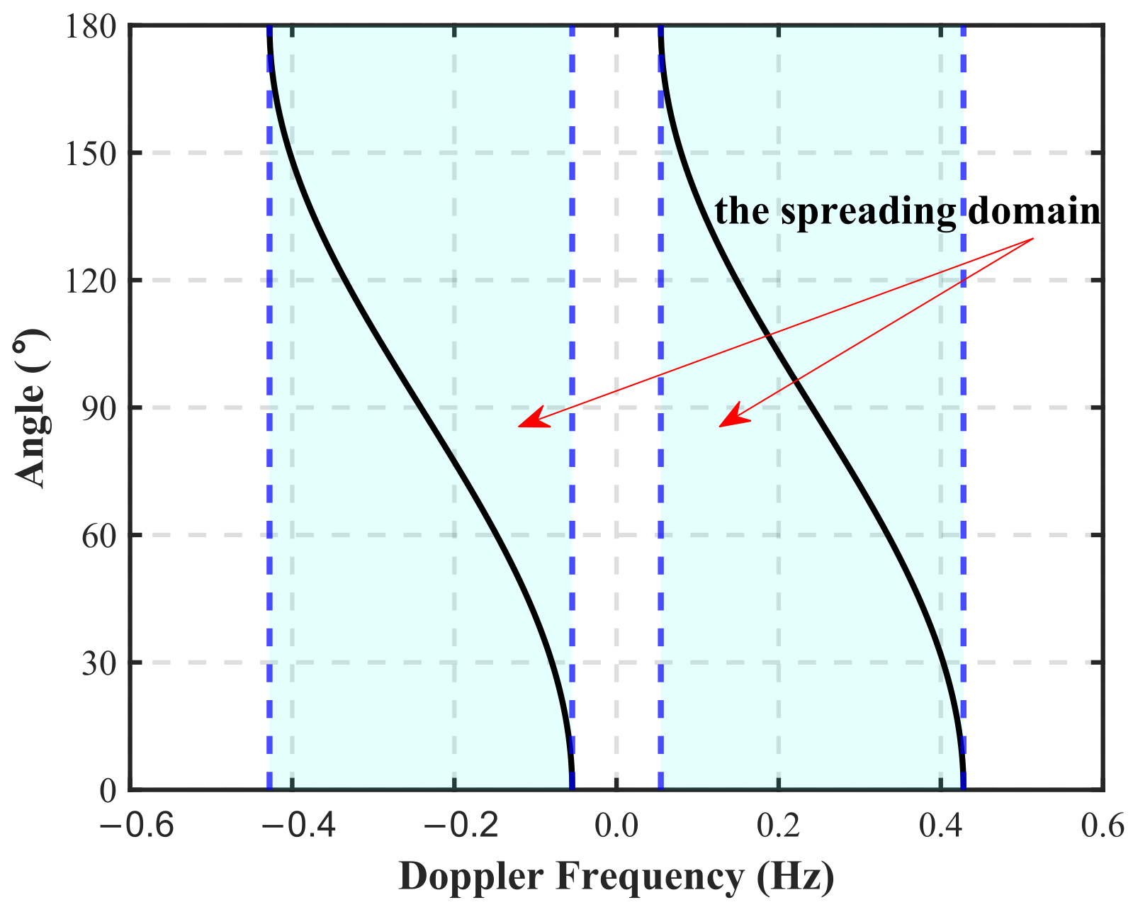
Therefore, sea cells at different azimuths introduce varying frequency shifts to the first-order Bragg peaks with onshore HFSWR, as demonstrated in Figure 1, which operates at a frequency of 5.6 MHz, with a shipborne speed of 5 m/s.

Given the space-constrained shipborne platform, a single antenna is optimal for both transmission and reception, which is the antenna configuration considered in this article. Ideally, the receiving antenna functions as a directional sensor with a single-side-looking characteristic ($\phi \in \left[0,\pi \right]$), as shown in Figure 2. As a result, the first-order Bragg peaks of shipborne HFSWR are spreading, represented by the blue-shaded region in Figure 1, with the spreading domains expressed as

$$\left[-f_B-2v/\lambda ,-f_B+2v/\lambda \right]\cup \left[f_B-2v/\lambda ,f_B+2v/\lambda \right]$$

(4)

From Equation (3), sea cells at different azimuths correspond to different frequencies of positive and negative first-order peaks, enabling the deduction of azimuth $\phi$

$$\phi =arccos\left({\displaystyle \frac{\left(f_d+f_B\right)·\lambda }{2v}}\right)$$

(5)

For the sea surface Doppler spectrum at a fixed range after pulse compression and Doppler processing, the spreading domains of the first-order Bragg peaks are determined from Equation (4) at first, then conducting precise identification at the specified azimuth via Equation (5).

2.2. Inversion of Wind Field Information

According to Equation (2), the sea cell at azimuth $\phi$, $R\left(\phi \right)$, defined as the ratio of positive to negative first-order Bragg peak intensities, can be derived as

$$R\left(\phi \right)=10lg{\displaystyle \frac{P\left(2vcos\phi /\lambda +f_B,\phi \right)}{P\left(2vcos\phi /\lambda -f_B,\phi \right)}}=10lg{\displaystyle \frac{G\left(\phi +\pi -\alpha \right)}{G\left(\phi -\alpha \right)}}$$

(6)

where $P\left(2vcos\phi /\lambda +f_B,\phi \right)$ and $P\left(2vcos\phi /\lambda -f_B,\phi \right)$ represent the intensities of the positive and negative first-order Bragg peaks, respectively. Notably, $R\left(\phi \right)$ is solely related to the directional factor G(_▪).

Consequently, substituting the modified cardioid model into Equation (6) yields

$$R\left(\phi \right)=10lg{\displaystyle \frac{\xi +\left(1-\xi \right)y^s}{\xi +\left(1-\xi \right){\left(1-y\right)}^s}}$$

(7)

where $\xi =0.004$ is the strength ratio of upwind to downwind returns [38], $y={sin}^2\left({\displaystyle \frac{\alpha -\phi }{2}}\right)$, and $s\in \left[1,10\right]$ is the spreading parameter related to wind speed [36]. Hereby, the possible wind direction $\alpha$ can be estimated as

$$\alpha =\phi \pm 2arcsin\left(\sqrt{y}\right)$$

(8)

where wind direction is ambiguous and associated with the spreading parameter. Under normal wind situations, given that sea cells at adjacent azimuths and the same range are independent [39,40] and display gradually varying wind directions and spreading parameters, the unique intersection of their relationship curves enables the determination of both wind direction and the spreading parameter [23]. Thus, wind directions can be inverted by traversing sea cells derived from Equation (5).

Since the radiation patterns of the transmitting and receiving antennas exert an identical effect on both positive and negative first-order Bragg peaks at the same azimuth, this influence cancels out in Equation (6), ensuring that distortions from the shipborne structure do not interfere with the extraction of wind direction, subsequent wind speed, and significant wave height.

Furthermore, the relationship between the spreading parameter and a parameter $\mu$ that denotes the momentum transfer from the local wind to the waves can be derived by Tyler et al. [36]

$$s=\left\{\begin{array}{cc}0.2{(\mu -0.1)}^{-1}& \mu >0.1\\ 2& \mu <0.1\end{array}\right.$$

(9)

where $\mu =C_{10}^{{\displaystyle \frac{1}{2}}}{U}_{10}/\left(\kappa V\right)$, $U_{10}$ is the wind speed at 10 m above the sea surface, $\kappa =0.4$ is the von Karman constant, $V={\left[gc/\left(4\pi ·{10}^6{f}_0\right)\right]}^{{\displaystyle \frac{1}{2}}}$ is the wave speed based on the dispersion relation of the sea surface, $c=3\times {10}^8\mathrm{m}/\mathrm{s}$, $g=9.8{\mathrm{m}/\mathrm{s}}^2$ is the acceleration due to gravity, and $f_0$ (MHz) is the radiation frequency.

Then, the drag coefficient $C_{10}=\left(0.8+0.065U_{10}\right)\times {10}^{-3}$, as proposed by Wu et al. [41], is applied to derive

$$\mu =\sqrt{{\displaystyle \frac{4\pi ·{10}^3{f}_0}{gc{\kappa }^2}}}·{\left(0.8+0.065U_{10}\right)}^{{\displaystyle \frac{1}{2}}}{U}_{10}$$

(10)

Employing the classic Cardano formula, wind speed can be solved as

$$\begin{array}{cc}\hfill & U_{10}={\left(A_{\mu }+\sqrt{B_{\mu }}\right)}^{{\displaystyle \frac{1}{3}}}+{\left(A_{\mu }-\sqrt{B_{\mu }}\right)}^{{\displaystyle \frac{1}{3}}}-4.1026\hfill \\ \hfill & A_{\mu }=-69.0504+2.8795·{10}^5{f}_0^{-1}{\mu }^2\hfill \\ \hfill & B_{\mu }=-3.9766·{10}^7{f}_0^{-1}{\mu }^2+8.2914·{10}^{10}{f}_0^{-2}{\mu }^4\hfill \end{array}$$

(11)

In the situation where $U_{10}>U^{*}$ ($U^{*}$ can be obtained by setting $\mu =0.1$ in Equation (11)), substituting Equation (9) into Equation (11) yields

$$\begin{array}{cc}\hfill & U_{10}={\left(A_s+\sqrt{B_s}\right)}^{{\displaystyle \frac{1}{3}}}+{\left(A_s-\sqrt{B_s}\right)}^{{\displaystyle \frac{1}{3}}}-4.1026\hfill \\ \hfill & A_s=-69.0504+2.8795·{10}^5{f}_0^{-1}{\left({\displaystyle \frac{0.2}{s}}+0.1\right)}^2\hfill \\ \hfill & B_s=-3.9766·{10}^7{f}_0^{-1}{\left({\displaystyle \frac{0.2}{s}}+0.1\right)}^2+8.2914·{10}^{10}{f}_0^{-2}{\left({\displaystyle \frac{0.2}{s}}+0.1\right)}^4\hfill \end{array}$$

(12)

Therefore, the spreading parameter can serve as an indicator of wind speed. By substituting the inverted spreading parameter into Equation (12), wind speed can be derived, achieving the inversion of wind field information from the spreading first-order Bragg peaks of shipborne HFSWR with a single antenna.

2.3. Extraction of Significant Wave Height

2.3.1. Significant Wave Height Extraction Method

For shipborne HFSWR, it is unable to extract significant wave height using onshore methods due to the spreading of first-order Bragg peaks and aliasing in the second-order Doppler spectrum. To address this, we propose a novel method that reverses the well-known onshore wind speed inversion route [42]. This route involves utilizing the relationship proposed by Sverdrup and Munk and modified by Bretshneider (SMB relationship), which is specially applied to relatively simple wind regimes, to derive wind speed from significant wave height, which is extracted from the aliasing-free second-order Doppler spectrum. Thus, wind speed, as derived from Equation (12), serves as the input to extract significant wave height.

The SMB relationship model can be expressed as [43]

$$H_s={\displaystyle \frac{0.26U_{10}^2}{g}}·tanh\left[{\displaystyle \frac{1}{{10}^2}}{\left({\displaystyle \frac{3.5g}{U_{10}{f}_m}}\right)}^{{\displaystyle \frac{3}{2}}}\right]$$

(13)

where $f_m$ is the spectral peak frequency that is usually obtained from the second-order Doppler spectrum.

Similar to significant wave height, $f_m$ cannot currently be directly obtained due to the characteristics of shipborne HFSWR. Consequently, in fully developed wind seas or developing wind seas with suitably large nondimensional fetch, the spectral peak frequency of the Pierson–Moskowitz (PM) spectrum $f_m={\left({\displaystyle \frac{4\beta }{5}}\right)}^{{\displaystyle \frac{1}{4}}}{\displaystyle \frac{g}{2\pi U_{19.5}}}$ [44] is employed as the approximation. Here, $U_{19.5}$ is the wind speed at 19.5 m above the sea surface; $\beta =0.74$ is a constant. As for the reliability of this approximation, it will be discussed in detail later.

Thus, Equation (13) can be modified to

$$H_s={\displaystyle \frac{0.26U_{10}^2}{g}}·tanh\left[{\displaystyle \frac{1}{{10}^2}}{\left({\displaystyle \frac{4\beta }{5}}\right)}^{-{\displaystyle \frac{3}{8}}}{\left(7\pi \right)}^{{\displaystyle \frac{3}{2}}}{\left({\displaystyle \frac{U_{19.5}}{U_{10}}}\right)}^{{\displaystyle \frac{3}{2}}}\right]$$

(14)

Additionally, the wind speed conversion at different heights above the sea surface can be expressed as [45]

$$U_z=U_{10}\left(1+{\displaystyle \frac{{C_{10}}^{\frac{1}{2}}}{\kappa }}ln{\displaystyle \frac{z}{10}}\right)$$

(15)

where z is the height above the sea surface.

Setting $z=19.5$ and substituting Equation (15) into Equation (14), the extracted significant wave height can be derived

$$H_s=0.0265U_{10}^2·tanh\left(1.2553·q^{{\displaystyle \frac{3}{2}}}\right)$$

(16)

in which

$$\begin{array}{c}\hfill q=1+0.0528{\left(0.8+0.065U_{10}\right)}^{{\displaystyle \frac{1}{2}}}\end{array}$$

2.3.2. Validation of the Approximation Replacement

For fully developed wind seas, wave characteristics can be typically described by the PM spectrum [44]

$$S_{PM}\left(K\right)={\displaystyle \frac{{\alpha }_{PM}}{{2K}^4}}exp\left[-\beta {\left({\displaystyle \frac{g}{K{U}_{19.5}^2}}\right)}^2\right]$$

(17)

where ${\alpha }_{PM}=0.0081$. The significant wave height $H_{sr}$ is determined by the integral of $S_{PM}\left(K\right)$ over K as [46]

$$H_{sr}=2\sqrt{{\displaystyle \frac{{\alpha }_{PM}}{\beta g^2}}}{U}_{19.5}^2$$

(18)

From Equation (15), the relationship between $H_{sr}$ and $U_{10}$ can be written as

$$H_{sr}=0.0214U_{10}^2{q}^2$$

(19)

Figure 3 illustrates the variation between extracted and actual significant wave heights as a function of wind speed under fully developed wind seas. Despite some discrepancies, the results exhibit general consistency. To quantify these differences, the relative error $\epsilon$ is defined as

$$\epsilon ={\displaystyle \frac{\left|H_s-H_{sr}\right|}{H_{sr}}}$$

(20)

Applying this definition, results indicate that the relative error gradually increases with wind speed but remains consistently below 10%, thus supporting the theoretical applicability of the approximation replacement.

Moreover, for developing wind seas, wave characteristics can be typically described by the JONSWAP spectrum [47]

$$S_{JONSWAP}\left(K\right)={\displaystyle \frac{{\alpha }_{JS}}{2K^4}}exp\left[-{\displaystyle \frac{5{\omega }_m^4}{g^2{K}^2}}\right]{\gamma }^{r\left(K\right)}$$

(21)

in which

$$\begin{array}{cc}& r\left(K\right)=exp\left[-{\left(\sqrt{gK}-{\omega }_m\right)}^2/\left(2{\sigma }^2{\omega }_m^2\right)\right]\hfill \\ & {\alpha }_{JS}=0.076{\tilde{L}}^{-0.22}\hfill \\ & {\omega }_m={\displaystyle \frac{22g}{U_{10}}}{\tilde{L}}^{-0.33}\hfill \\ & \sigma =\left\{\begin{array}{cc}& 0.07,\begin{array}{cc} & \omega \le {\omega }_m\end{array}\hfill \\ & 0.09,\begin{array}{cc} & \omega >{\omega }_m\end{array}\hfill \end{array}\right.\hfill \end{array}$$

where $\gamma =3.3$ represents the peak enhancement factor and the relationship between the nondimensional fetch, $\tilde{L}$, and fetch, L, is given by $\tilde{L}={\displaystyle \frac{gL}{U_{10}^2}}$. After integral, the significant wave height $H_{sr}$ can be written as

$$H_{sr}=0.4082U_{10}^2\sqrt{1.67\times {10}^{-7}\tilde{L}}$$

(22)

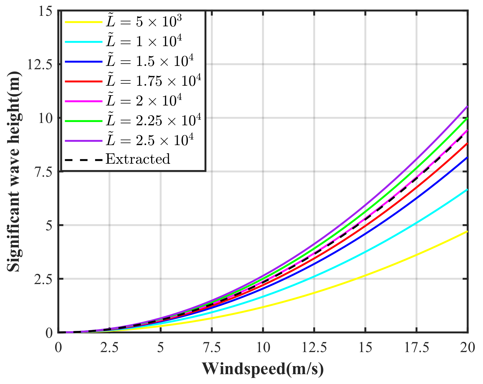
Figure 4 presents extracted significant wave heights, along with actual significant wave heights for various values of $\tilde{L}$ as a function of wind speed. When $\tilde{L}\approx 2\times {10}^4$, the extracted and actual values are in full agreement. However, deviations in $\tilde{L}$—whether too high or too low—introduce errors in significant wave heights extracted from Equation (16). To establish criteria for approximation feasibility, the upper limit of relative error, ${\epsilon }_{max}$, is defined based on specific experimental accuracy requirements. Here, ${\epsilon }_{max}$ is set to 20%, serving as a reasonable acceptable threshold. For developing wind seas, the approximation replacement requires $\tilde{L}$ to fall within (1.37–3.05) × ${10}^4$ to ensure $\epsilon \le {\epsilon }_{max}$.

Therefore, this approximation replacement is applicable to fully developed wind seas and to developing wind seas that meet certain nondimensional fetch conditions under specific accuracy requirements.

2.4. Theoretical Error Analysis

External noise and computer discretization errors introduce inaccuracies in the spreading parameter inversion results. Given the indirect nature of the proposed significant wave height extraction method, errors in the spreading parameters propagate to significant wave heights from wind speeds. Consequently, a quantitative analysis of the impact of the spreading parameter error on significant wave height is essential.

The derivative $H_s^{\prime }$ of the extracted significant wave height concerning the spreading parameter can be written as

$$H_s^{\prime }={\displaystyle \frac{d{H}_s}{ds}}={\displaystyle \frac{d{H}_s}{d{U}_{10}}}·{\displaystyle \frac{d{U}_{10}}{ds}}={\displaystyle \frac{\mathsf{\Delta }{H}_s}{\mathsf{\Delta }s}}$$

(23)

where $\mathsf{\Delta }{H}_s$ and $\mathsf{\Delta }s$ represent the variations in significant wave height and spreading parameter, respectively.

The term ${\displaystyle \frac{dHs}{d{U}_{10}}}$, derived from Equation (16) with its negligible second term omitted, can be simplified as

$${\displaystyle \frac{d{H}_s}{d{U}_{10}}}\approx 0.0531U_{10}·tanh\left(1.2553·q^{{\displaystyle \frac{3}{2}}}\right)$$

(24)

In addition, the term ${\displaystyle \frac{d{U}_{10}}{ds}}$ can be derived from Equation (12) as

$$\begin{array}{cc}\hfill & {\displaystyle \frac{d{U}_{10}}{ds}}={\displaystyle \frac{\left(A_s^{\prime }+\frac{B_s^{\prime }}{2\sqrt{B_s}}\right)}{3{\left(A_s+\sqrt{B_s}\right)}^{\frac{2}{3}}}}+{\displaystyle \frac{\left(A_s^{\prime }-\frac{B_s^{\prime }}{2\sqrt{B_s}}\right)}{3{\left(A_s-\sqrt{B_s}\right)}^{\frac{2}{3}}}}\hfill \\ \hfill & A_s^{\prime }=-1.1518·{10}^5{f}_0^{-1}{s}^{-2}\left({\displaystyle \frac{0.2}{s}}+0.1\right)\hfill \\ \hfill & B_s^{\prime }=1.5906·{10}^7{f}_0^{-1}{s}^{-2}\left({\displaystyle \frac{0.2}{s}}+0.1\right)-6.6331·{10}^{10}{f}_0^{-2}{s}^{-2}{\left({\displaystyle \frac{0.2}{s}}+0.1\right)}^3\hfill \end{array}$$

(25)

To quantitatively assess the propagation of relative error, the relative error ratio $k_{H-s}$ between the significant wave height and the spreading parameter can be defined as

$$k_{H-s}={\displaystyle \frac{\left|\mathsf{\Delta }{H}_s/H_s\right|}{\left|\mathsf{\Delta }s/s\right|}}=\left|{\displaystyle \frac{s{H}_s^{\prime }}{H_s}}\right|$$

(26)

where $\left|{\displaystyle \frac{\mathsf{\Delta }{H}_s}{H_s}}\right|$ and $\left|{\displaystyle \frac{\mathsf{\Delta }s}{s}}\right|$ represent the relative errors in significant wave height and the spreading parameter.

Substituting Equation (23) into (26) yields

$$k_{H-s}\approx \left|{\displaystyle \frac{0.6667s\left[\left(A_s^{\prime }+\frac{B_s^{\prime }}{2\sqrt{B_s}}\right)·{\left(A_s+\sqrt{B_s}\right)}^{-\frac{2}{3}}+\left(A_s^{\prime }-\frac{B_s^{\prime }}{2\sqrt{B_s}}\right)·{\left(A_s-\sqrt{B_s}\right)}^{-\frac{2}{3}}\right]}{{\left(A_s+\sqrt{B_s}\right)}^{\frac{1}{3}}+{\left(A_s-\sqrt{B_s}\right)}^{\frac{1}{3}}-4.1026}}\right|$$

(27)

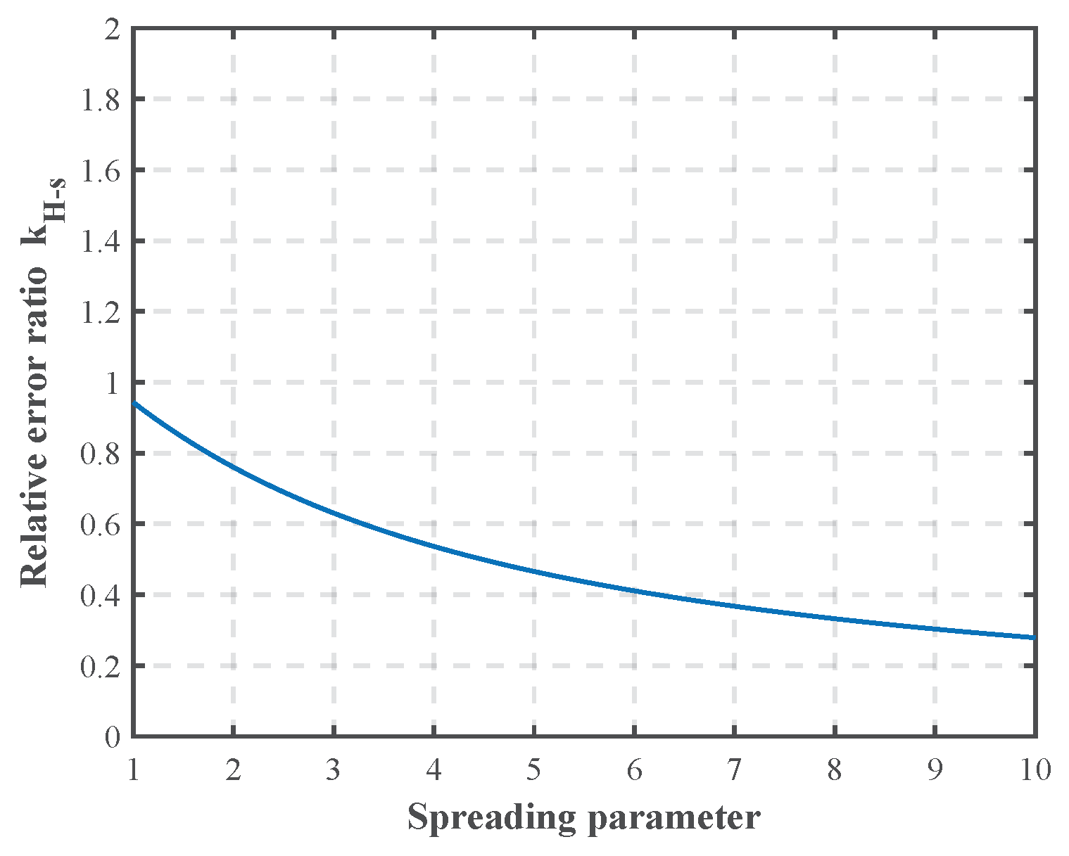
Equation (27) consistently satisfies $k_{H-s}<1$, reflecting the tolerance of the significant wave height extraction process to the input errors, as illustrated in Figure 5 with a radiation frequency of 5.6 MHz as an example. However, if the inverted spreading parameter is an outlier, its relative error increases significantly, and, although the relative error in the significant wave height is reduced compared to the input, it may remain unacceptably high. Thus, controlling the occurrence of spreading parameter outliers is essential.

2.5. The Spreading Parameter Preprocessing

When the significant wave height is indirectly extracted from the spreading parameter, the presence of an outlier will introduce a relative error in the significant wave height that, although reduced compared to that of the spreading parameter, remains substantial. To overcome this, a preprocessing step for the spreading parameter is proposed before the wind speed inversion process to minimize the occurrence of outliers. The specific steps are as follows:

Step1: As shown in Figure 6, the spreading parameter of each sea cell is extracted based on the radar azimuth and detection range.

Step2: The distribution of the spreading parameters is determined, and the spreading parameter level is assessed. Based on this, the acceptable range is set, the spreading parameters of sea cells within this range are recorded, and the mean of these values is calculated.

Step3: If the spreading parameter of a sea cell on the detection boundary exceeds the range, it is substituted with the mean calculated in Step2.

Step4: If the spreading parameter of a sea cell within the internal detection area exceeds the range, it is replaced with the average spreading parameter of the adjacent sea cells (such as O in Figure 6, where the adjacent cells are A, B, C, and D). If the spreading parameter of an adjacent cell also exceeds the range, it is temporarily substituted with the mean calculated in Step2.

Step5: All sea cells within the detection area are traversed to reduce the occurrence of outliers in the spreading parameters.

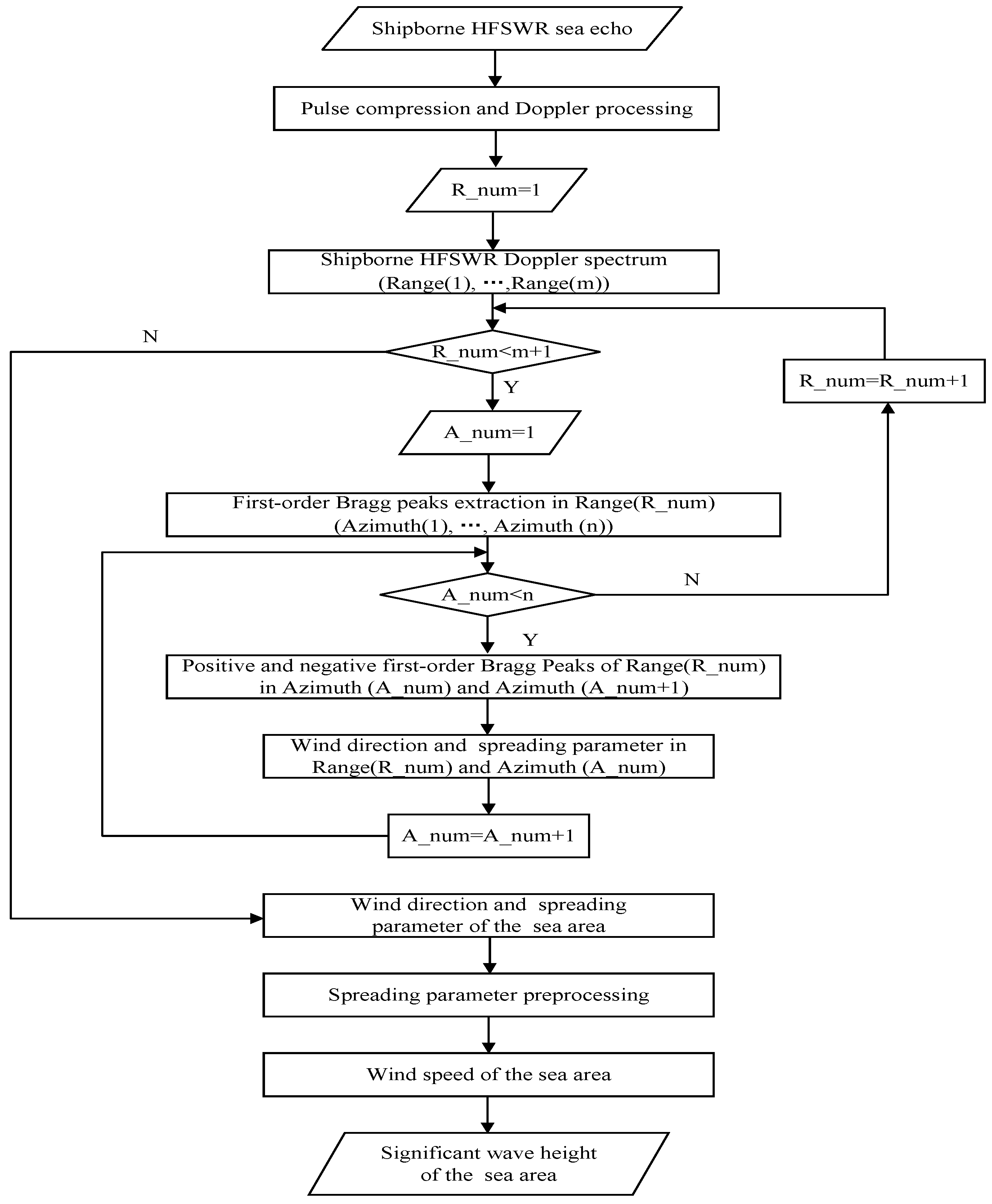
Thus far, a complete process for extracting significant wave height from the spreading first-order peaks of shipborne HFSWR with a single antenna has been proposed, as shown in Figure 7. Theoretically, this method applies to both fully developed wind seas and developing wind seas that meet the conditions outlined in Section 2.3.2.

3. Simulation and Analysis

3.1. Simulation Results

In the simulation, the radiation frequency $f_0$ is set to 5.6 MHz, the threshold $U^{*}$ calculated from Equation (11) is 7.25 m/s, the shipborne speed v is 5 m/s, the wind direction over the sea area is assumed to be uniform, and the directional factor is based on the assumption outlined in Section 2.1. For fully developed wind seas, Equation (17) is applied to the nondirectional wave spectrum in Equation (1), while, for developing wind seas, Equation (21) is used.

Figure 8 presents the simulated spreading first-order Bragg peaks under 8 different wind-sea conditions (see

Table 1. Eight different wind-sea conditions.

Condition	State	Wind Direction	Spreading Parameter	Wind Speed	Nondimensional Fetch	Significant Wave Height
1	Fully developed	45°	2	12.80 m/s		4.00 m
2	Fully developed	315°	2	12.80 m/s		4.00 m
3	Fully developed	45°	4	10.15 m/s		2.50 m
4	Fully developed	315°	4	10.15 m/s		2.50 m
5	Developing	45°	2	12.80 m/s	$2\times {10}^4$	3.87 m
6	Developing	315°	2	12.80 m/s	$2\times {10}^4$	3.87 m
7	Developing	45°	4	10.15 m/s	$2\times {10}^4$	2.43 m
8	Developing	315°	4	10.15 m/s	$2\times {10}^4$	2.43 m

for details). For developing wind seas, the approximately optimal case of $\tilde{L}\approx 2\times {10}^4$, as discussed in Section 2.3.2, is defined, while non-ideal conditions are discussed subsequently. Wind speeds and significant wave heights are set according to Equations (12), (19), and (22).

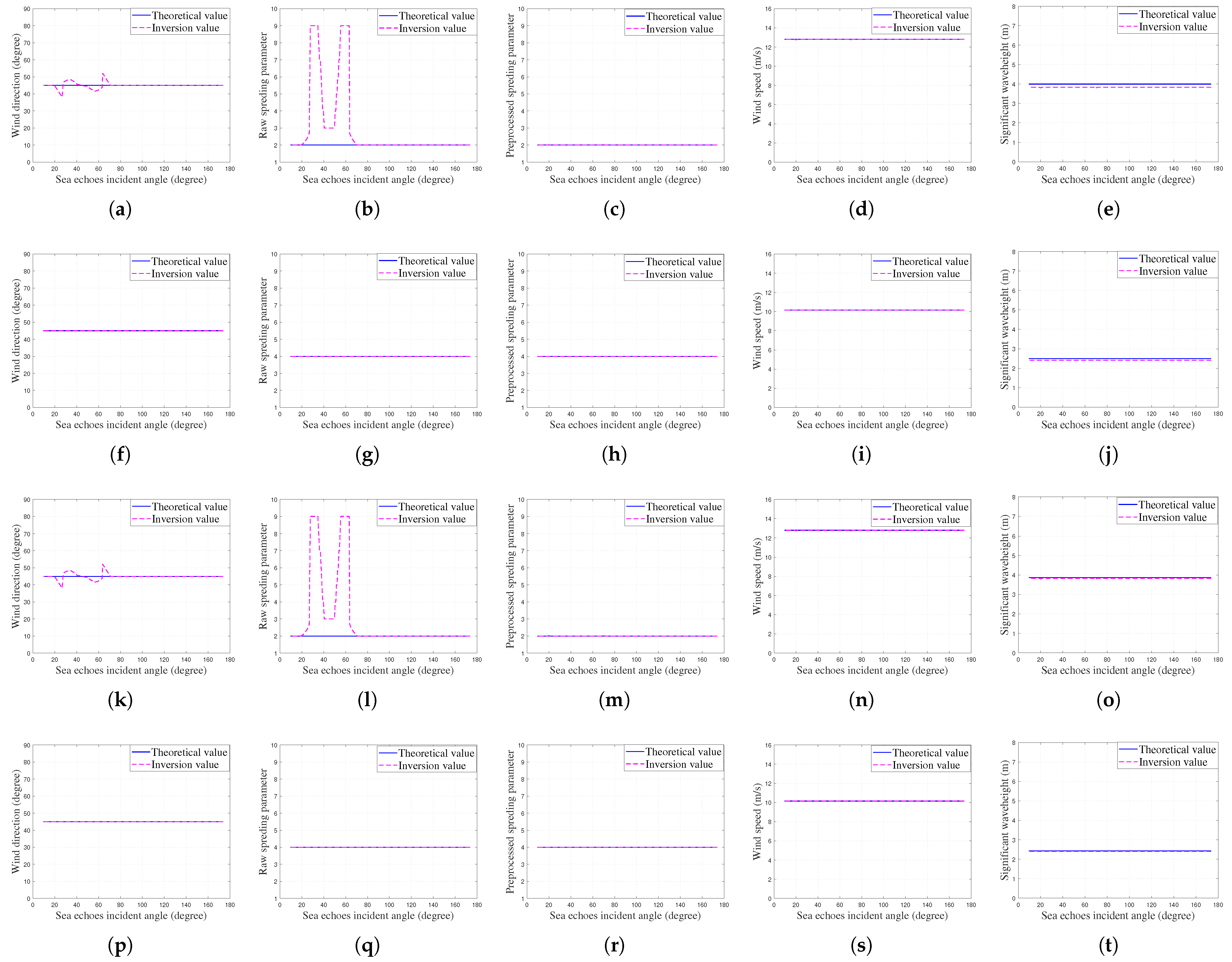
Different characteristics in the spreading first-order Bragg peaks are exhibited under each wind-sea condition, with wind speeds exceeding the threshold $U^{*}$, indicating that these spreading peaks can be used to extract sea state information. Under wind-sea conditions 1, 3, 5, and 7, wind directions, raw and preprocessed spreading parameters, wind speeds, and significant wave heights are extracted based on the proposed method, with the results depicted in Figure 9.

The simulation results indicate that, under wind-sea conditions 1 and 5, the inverted wind directions show minor fluctuations compared to the given values, yet these fluctuations remain within acceptable limits. Computer discretization errors result in some inverted spreading parameters appearing as outliers, which, if used directly, will significantly impact the final results. By applying preprocessing to spreading parameters, most outliers are effectively mitigated, affirming the effectiveness of this step. The extracted wind speeds and significant wave heights demonstrate consistency with the given values. Under wind-sea conditions 3 and 7, the extracted wind field and wave height information align closely with the given data. These results preliminary validate the feasibility and potential of the proposed method.

3.2. Application Analysis

3.2.1. The Influence of Current

The spreading first-order Bragg peaks described by Equation (1) represent an ideal case that does not account for the ocean current. However, ocean current is a critical parameter of the sea area. Assume a uniform radial current and the first-order Bragg peaks are modified as

$$\sigma \left(f_d,\phi \right)=2^6{\pi }^2{k}_0^4\sum _{m=\pm 1}S\left(2k_0\right)G\left(\phi +\psi -\alpha \right)·\delta \left(f_d+m{f}_B-{\displaystyle \frac{2v}{\lambda }}cos\phi -{\displaystyle \frac{2v_c}{\lambda }}\right)$$

(28)

where the radial current $v_c$ ultimately induces a frequency shift in the spreading first-order Bragg peaks of the shipborne HFSWR, given by $\mathsf{\Delta }f={\displaystyle \frac{2v_c}{\lambda }}$, which impacts accurate identification of the first-order Bragg peaks at the specific azimuth and thereby subsequent wind and wave information extraction.

To address this issue, integrated compensation is applied to mitigate the influence of a uniform radial current by observing the boundaries of the affected first-order Bragg peaks and shifting them to the ideal positions described in Equation (4). Results before and after compensation, shown in Figure 10a,b for wind-sea condition 1, confirm the effectiveness of the compensation as the first-order Bragg peaks are restored to their ideal state. Therefore, after applying the integrated compensation, the radial ocean current has little to no effect on the significant wave height extraction.

3.2.2. The Influence of Nondimensional Fetch

For wind-sea conditions 5 and 7, the nondimensional fetch $\tilde{L}$ is set to be $2\times {10}^4$, representing the approximately optimal case discussed in Section 2.3.2, to simulate the extraction method. In practical situations, however, $\tilde{L}$ usually deviates from this ideal, potentially introducing inaccuracies in the extraction results. Accordingly, for effective extraction, the conditions that $\tilde{L}$ should meet are examined. 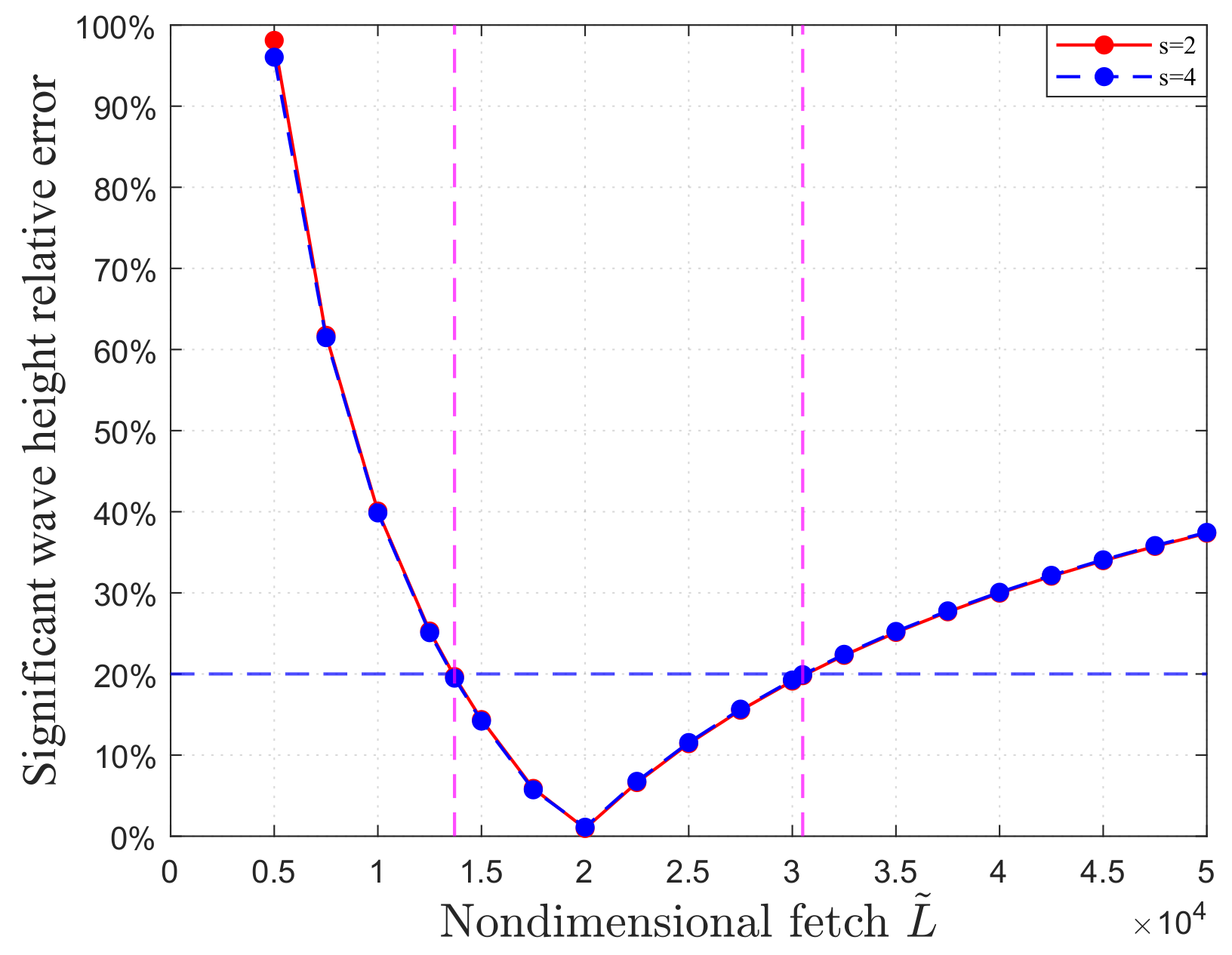Various values of $\tilde{L}$ are simulated to assess the performance of the proposed method, with other simulation parameters held consistent with wind-sea conditions 5 and 7. The derived relative errors in significant wave height are shown in Figure 11.

The effect of the spreading parameter on extraction is negligible, whereas $\tilde{L}$ has a significant impact on the extraction, with the relative error close to 0 when $\tilde{L}\approx 2\times {10}^4$ and remaining below 20% within the range (1.37–3.05) × ${10}^4$. However, if $\tilde{L}$ deviates significantly from this range, the relative error increases sharply, rendering the extraction method invalid. These results align with the theoretical analysis in Section 2.3.2.

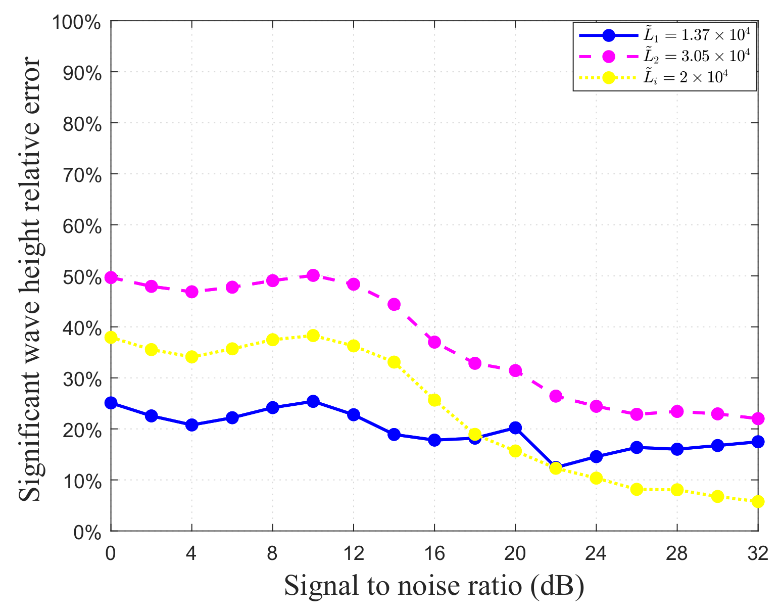
3.2.3. The Influence of Noise

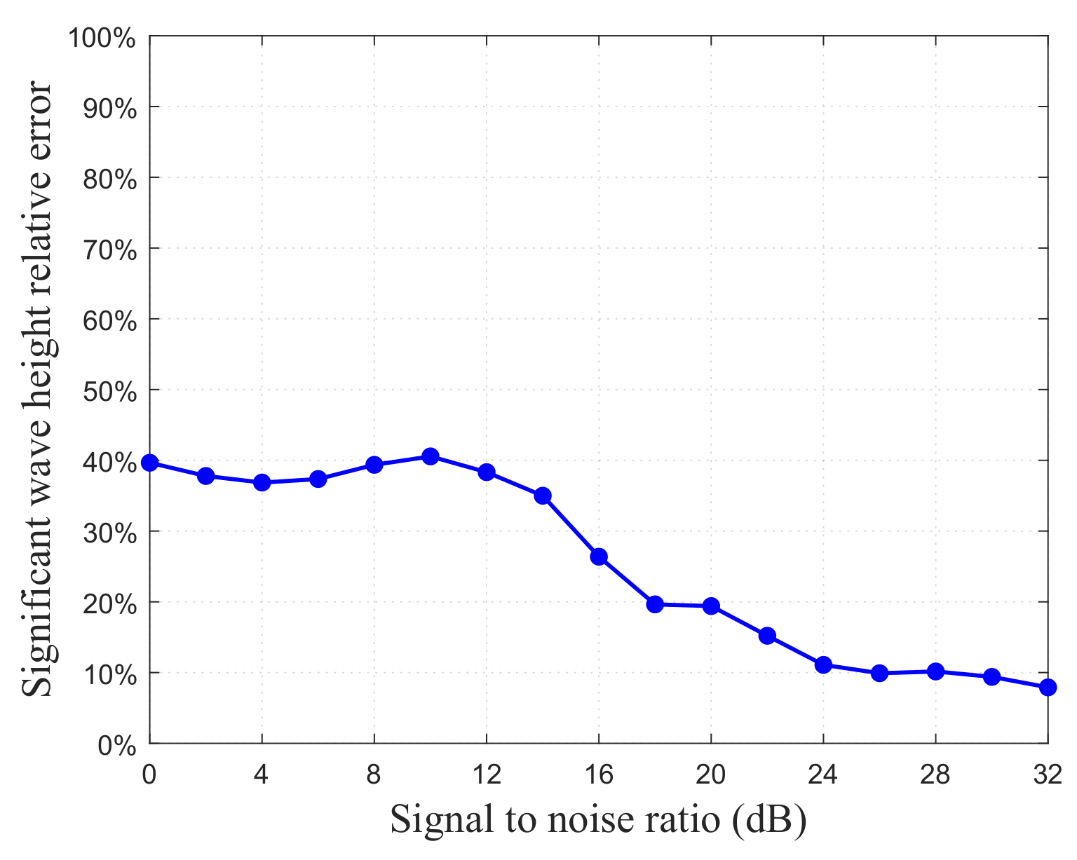
It is well known that external noise is inevitable. Taking wind-sea condition 1 as an example, Figure 12 presents the simulated first-order Bragg peaks with and without noise. As the SNR decreases, noise amplifies fluctuations in the spreading first-order Bragg peaks, thereby negatively impacting the subsequent extraction of wind and wave field information. To assess the effect of external noise on the extracted significant wave height and account for noise randomness, 100 Monte Carlo simulations are performed for each SNR under wind-sea condition 1.

The relative errors of extracted significant wave heights are shown in Figure 13, indicating that noise has a significant impact on the extraction accuracy. With increasing SNR, relative errors generally decrease. Specifically, when SNR exceeds 16 dB, the relative error falls below 30%, and, at SNR levels above 18 dB, it further decreases to under 20%. Therefore, 18 dB can be considered a threshold for obtaining reliable extraction results in fully developed wind seas. With continued increases in SNR, the relative error approaches 10%, as discussed in Section 2.3.2.

3.2.4. The Influence of Shipborne Structure

A shipborne platform model is used to assess how its structure influences the radiation patterns of the transmitting and receiving antennas. Measuring 150 m in length, 20 m in width, and 20 m in height at the deck, the platform features a surface composed of a perfect electric conductor. The transmitting antenna is centrally installed on the platform, while the receiving antenna is set on the offshore side, either to the left or right. 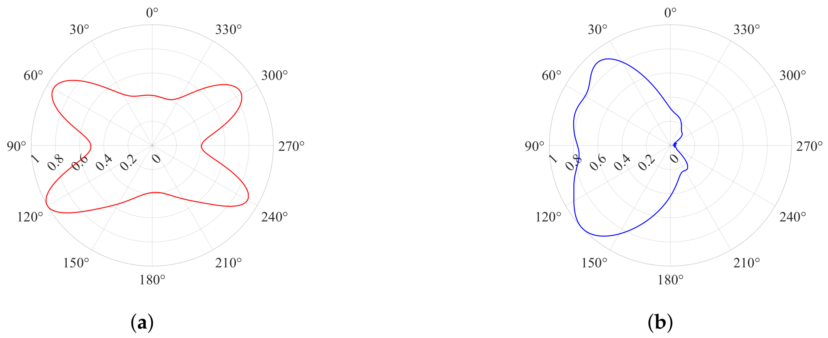Figure 14 depicts the simulated distorted normalized radiation patterns for both antennas, and Figure 15a presents the spreading first-order Bragg peaks under wind-sea condition 1, which differ from those in Figure 8a. The extracted significant wave heights are displayed in Figure 15b, which are entirely consistent with the undistorted case. Therefore, antenna distortion is not considered to be a factor affecting the accuracy of significant wave height extraction. These findings confirm that distortions in antenna patterns due to the shipborne structure do not impact the extraction process, highlighting a key advantage of the proposed method.

3.2.5. The Influence of Comprehensive Factors

Based on the current in Figure 10a, the influence of the minimum and maximum non-ideal nondimensional fetches, ${\tilde{L}}_1\approx 1.37\times {10}^4$ and ${\tilde{L}}_2\approx 3.05\times {10}^4$ (within a relative error limit of 20%), as well as the ideal nondimensional fetch ${\tilde{L}}_i=2\times {10}^4$, and external noise, are analyzed for their effects on extraction results under developing wind seas. For each SNR in Figure 13, 100 Monte Carlo simulations are performed, with other simulation parameters consistent with wind-sea condition 5. The relative errors of extracted significant wave heights are shown in Figure 16. Relative errors remain below 30% under ${\tilde{L}}_1$, and, for ${\tilde{L}}_2$ at low SNR, errors are greatly higher than in the other two cases, with noise being the dominant factor. As SNR increases, the influence of noise diminishes, and the error curves for ${\tilde{L}}_1$ and ${\tilde{L}}_2$ converge to around 20%, while the error approaches 0 for ${\tilde{L}}_i$, aligning with the theoretical analysis. Figure 16 also indicates that acceptable results are achieved when SNR exceeds 24 dB for developing wind seas that satisfy $\tilde{L}\approx \left(1.37\sim 3.05\right)\times {10}^4$.

4. Experimental Results and Analysis

Data from two shipborne HFSWR field experiments are used to verify the feasibility of the proposed extraction method, with radar system parameters for each experiment provided in

Table 2. Radar system parameters.

Parameter	Experiment 1	Experiment 2
Operating frequency (MHz)	6.45	5.6
Bandwidth (kHz)	50	30
Pulse repetition period (s)	0.252	0.252
Azimuth range (degree)	42.4–140.4	43.7–137.3
Detection range (km)	30–120	30–120
Range resolution (km)	3	5
Pulse integration number	512	512

. Both experiments were conducted in the West Taiwan Strait, and the shipborne real-time location was recorded by the Global Positioning System (GPS).

4.1. Data Description

4.1.1. Experiment 1

The experiment was conducted from 8:51:02 to 8:55:41 Beijing time on 26 September 2016 as the shipborne sailed southwest along the coastline, starting at (118°10′48″E, 24°13′06″N) and ending at (118°10′39″E, 24°12′24″N), with an average speed of 4.7 m/s. Sliding window processing with a step of 128 pulses is applied to obtain more real-time data, producing five datasets from two sets of raw data. Given the randomness of the sea echoes [39], a data averaging process is proposed for shipborne HFSWR: First, all first-order Bragg peaks are identified from the sliding window data. Then, considering the motion characteristics and range/angle resolutions of the shipborne HFSWR, the detection area is divided into grids with a 5° angle resolution and a 3 km range resolution. Finally, the averages of all the first-order Bragg peaks within each grid are calculated. During the experiment, the sea state was relatively stable. Specifically, the wind in the detection area blew from the north-northeast offshore for at least 72 h, fully developing the wind sea, and the wind speed changed slowly and exceeded the threshold $U_1^{*}$ = 7.25 m/s, as calculated by Equation (11).

4.1.2. Experiment 2

The experiment took place from 20:40:15 to 21:29:43 Beijing time on 3 December 2016, with the starting and ending positions at (118°55′19″E, 24°38′25″N) and (119°01′27″E, 24°43′54″N), respectively, and an average speed of 4.9 m/s. The 18 raw datasets are divided into four stages according to course and measurement time, as shown in

Table 3. Course and measurement time details in Experiment 2.

Stage	Starting Time	End Time	Course (North-Northeast)	Data
1	20:40:15	20:59:50	50.48°	Data 1–Data 8
2	21:00:10	21:14:47	40.15°	Data 9–Data 14
3	21:15:07	21:17:16	43.13°	Data 15
4	21:22:36	21:29:43	44.56°	Data 16–Data 18

. A sliding window with a step of 128 pulses is applied within each stage, resulting in a final total of 60 datasets. Given the extended duration of the experiment, data are grouped at 10 min intervals (20:35–20:45, …, 21:25–21:35), and the averaging process described above is performed with a range resolution of 5 km and an angle resolution of 5°. Additionally, a wave buoy was deployed at (119°17′24″E, 24°28′48″N) to measure significant wave heights in real time at 10 min intervals (20:50, …, 21:30 on 3 December 2016), and the accuracy of the extracted results can be verified by comparing the buoy with the nearest HFSWR measurements. Throughout the experiment, the buoy remained within the detection area, and the sea state was relatively stable. Specifically, the wind from the north-northeast blew offshore for at least 72 h, ensuring full development of the wind sea. The wind speed in the detection area changed slowly and exceeded the threshold $U_2^{*}$ = 6.83 m/s.

4.2. Experimental Results

To verify the performance of the proposed method, the significant wave height data from the fifth-generation European Centre for Medium-Range Weather Forecasts reanalysis (ERA5) hourly dataset is cited as a reference [48]. The ERA5 data combine forecasts from numerical weather prediction centers with newly available observations to optimally produce high-quality data, providing atmospheric data at a resolution of 0.25° × 0.25° in latitude and longitude and wave data at a resolution of 0.5° × 0.5°. The inverse distance weighting interpolation method [49] is used to obtain ERA5 significant wave height at the specific longitude and latitude position for comparison with the extracted significant wave height. The inverse distance weighting interpolation process is as follows:

Step 1: Calculate the distance from the position of interpolated data to every position of ERA5 data:

$$d_i=\sqrt{{(a-a_i)}^2+{(b-b_i)}^2}$$

where $(a,b)$ is the rectangular coordinate of the position of interpolated data, and $(a_i,b_i)$ is the rectangular coordinate of the position of ERA5 data.

Step 2: Calculate the weight value of every position of ERA5 data:

$$w_i={\displaystyle \frac{1/d_i}{{\displaystyle \sum _{i=1}^m}(1/d_i)}}$$

where m is the number of ERA5 data points.

Step 3: Calculate the value of the interpolated data:

$$Z_0=\sum _{i=1}^m{w}_i\ast Z(a_i,b_i)$$

where $Z(a_i,b_i)$ is the value of the ERA5 data.

The extraction results are objectively evaluated by calculating the mean relative error (MRE) and root mean square error (RMSE), with the statistical parameters calculated as follows

$$MRE={\displaystyle \frac{1}{n}}\sum _{i=1}^n\left|{\displaystyle \frac{x_i-X_i}{X_i}}\right|$$

(29)

$$RMSE={\left({\displaystyle \frac{1}{n}}\sum _{i=1}^n(x_i-X_i)\right)}^{1/2}$$

(30)

where n is the number of samples, $x_i$ and $X_i$ are the extracted and real significant wave height.

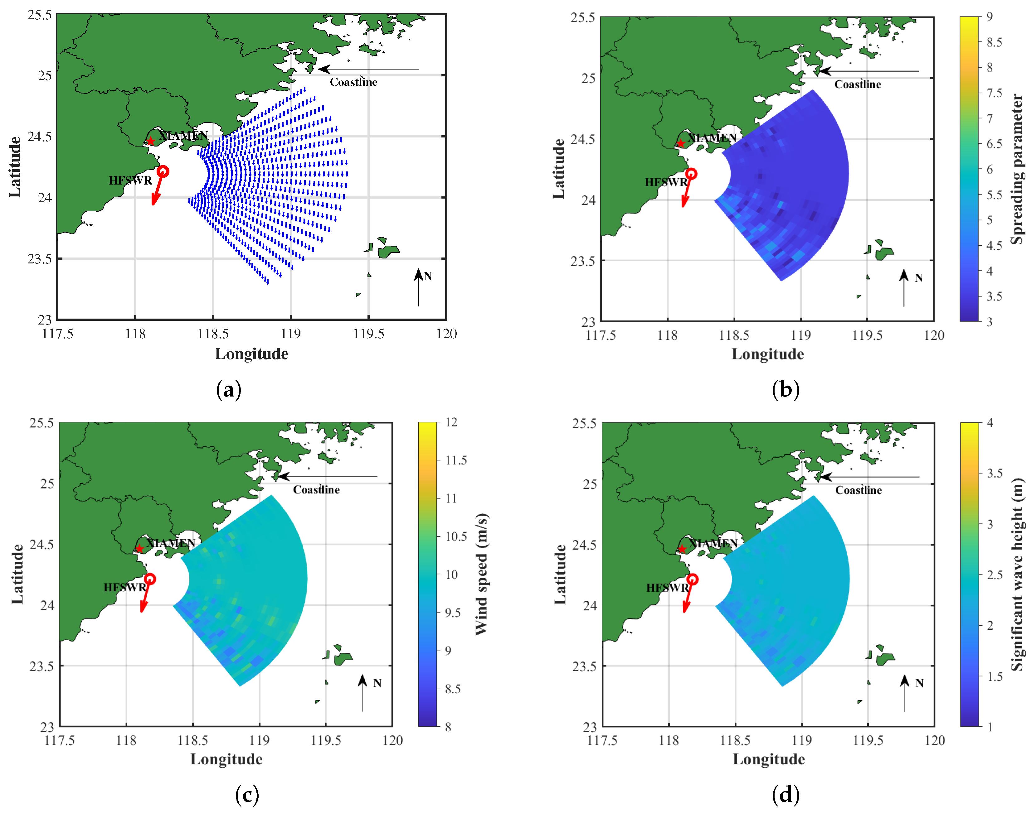
4.2.1. Experiment 1

Figure 17 presents the distribution of the extracted wind and wave field data, where the red arrow indicates the traveling direction of the shipborne HFSWR, and the red circle marks its initial position (the same applies to Figures 18, 20 and 21). The wind directions are predominantly north-northeast, consistent with the observed data. After preprocessing, the spreading parameters range from 3 to 5, with the majority centered around 3.5. The wind speeds vary between 9 and 11 m/s, with a central tendency near 10 m/s, while the significant wave heights range from 1.9 to 2.6 m, centered around 2.3 m.

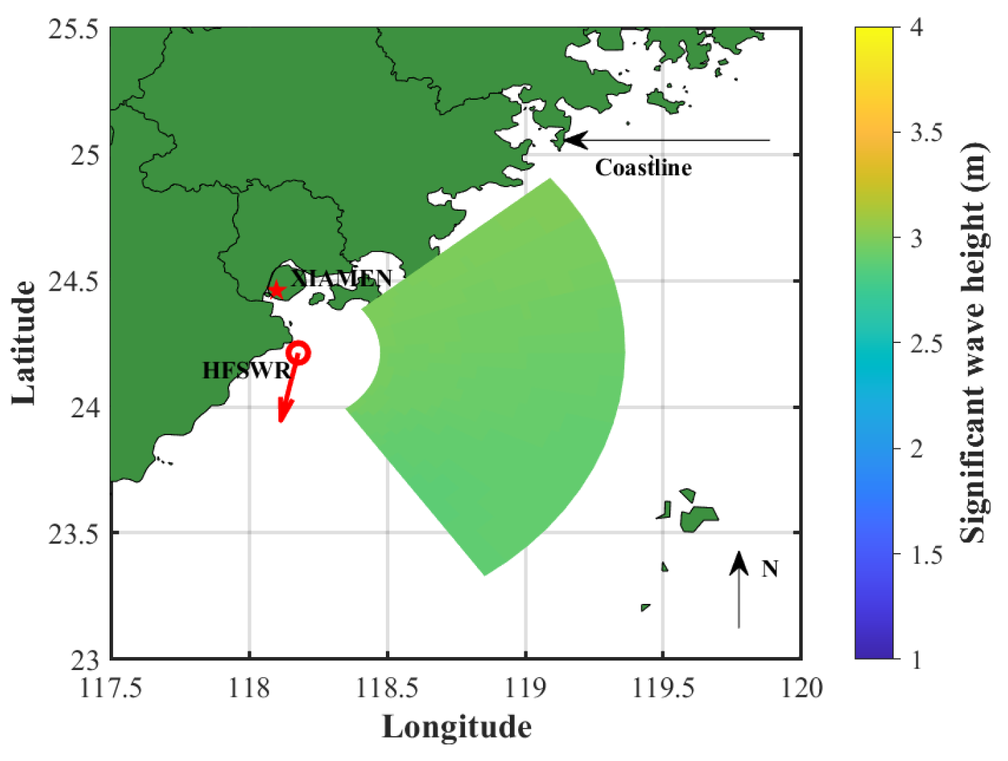
Considering the time of the experiment, the interpolated ERA5 significant wave heights at 9:00, as shown in Figure 18, are used to verify the extraction results. Figure 19 presents the comparison scatterplots. There are 620 significant wave height data samples, indicating that the extracted results are generally lower and more dispersed than the ERA5 reference data, with an MRE and RMSE of 22.62% and 0.6711 m, respectively. Given the performance of HFSWR in significant wave height extraction, this result is considered to be acceptable.

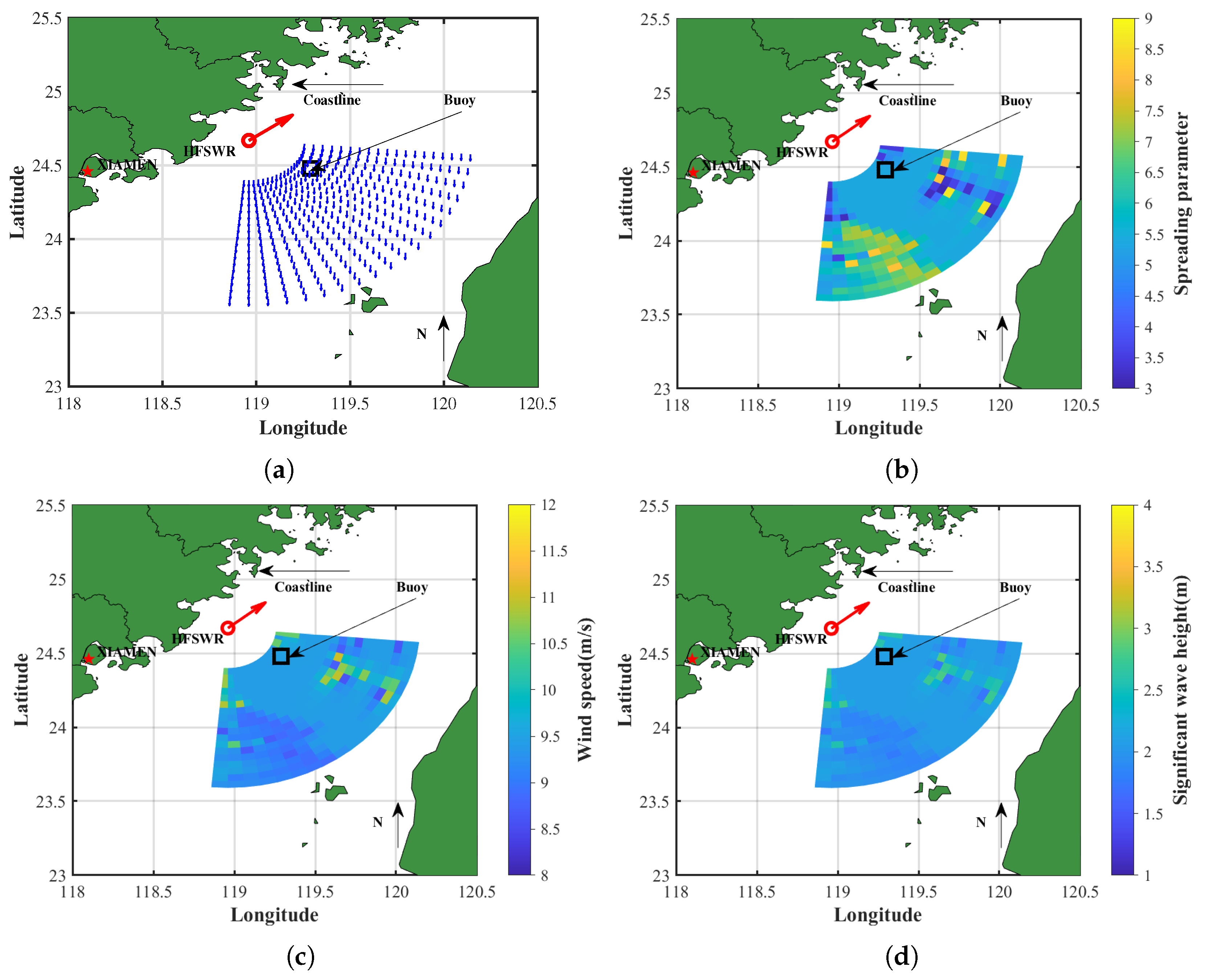
4.2.2. Experiment 2

Using the third averaged data group, Figure 20 illustrates the distributions of the extracted wind and wave field information. All the wind directions are north-northeast, consistent with the observations. The spreading parameters range from 3 to 9, with most values centered around 5.3. The wind speeds vary between 8 and 11 m/s, centered around 9.5 m/s, while the extracted significant wave heights range from 1.8 to 2.6 m, centered near 2.1 m. Figure 21 shows the distribution of interpolated ERA5 significant wave heights within the detection area of this data group at 21:00, with MRE and RMSE at 10.94% and 0.2777 m, respectively.

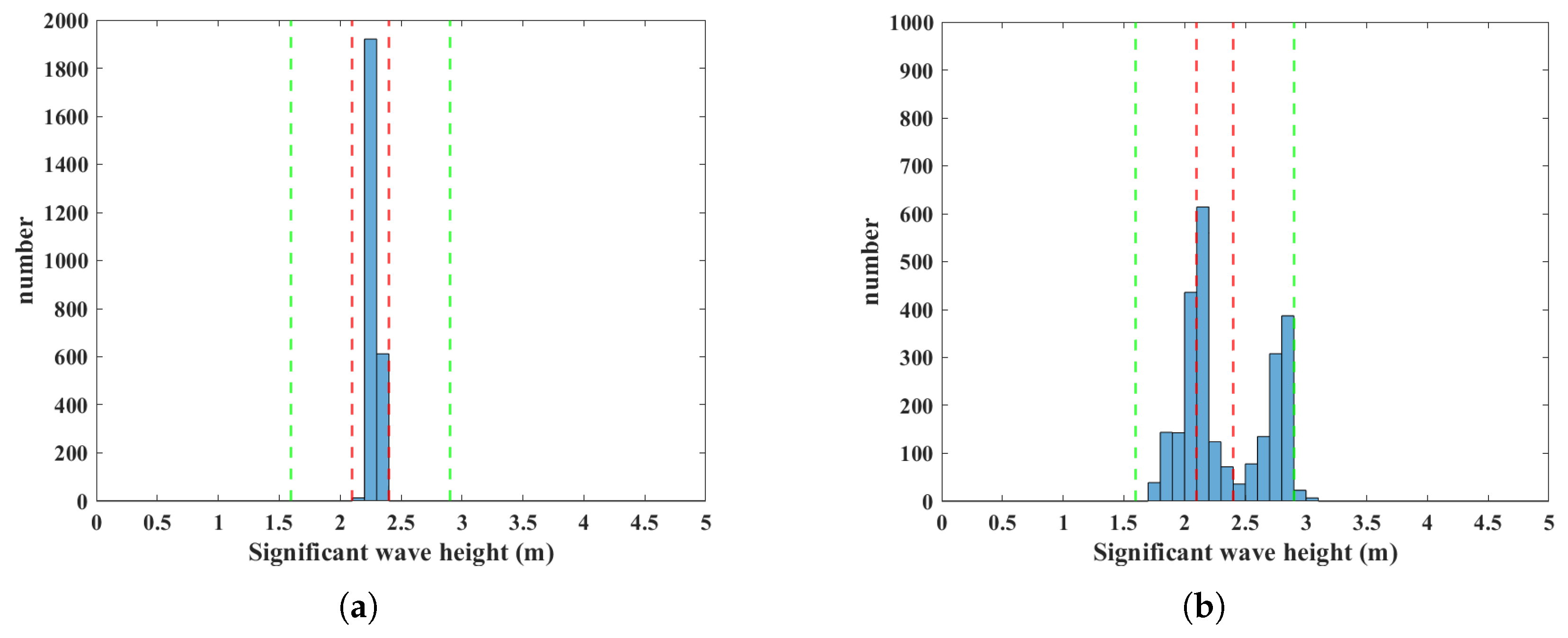
In Experiment 2, all the data groups yield a total of 2546 significant wave height samples. Figure 22 presents the histograms of the interpolated ERA5 and extracted significant wave heights. All the ERA5 reference data fall within the range of 2.1 to 2.4 m, represented by the red dashed lines in Figure 22, while the extracted significant wave heights are more dispersed, with approximately 31.81% within this range. 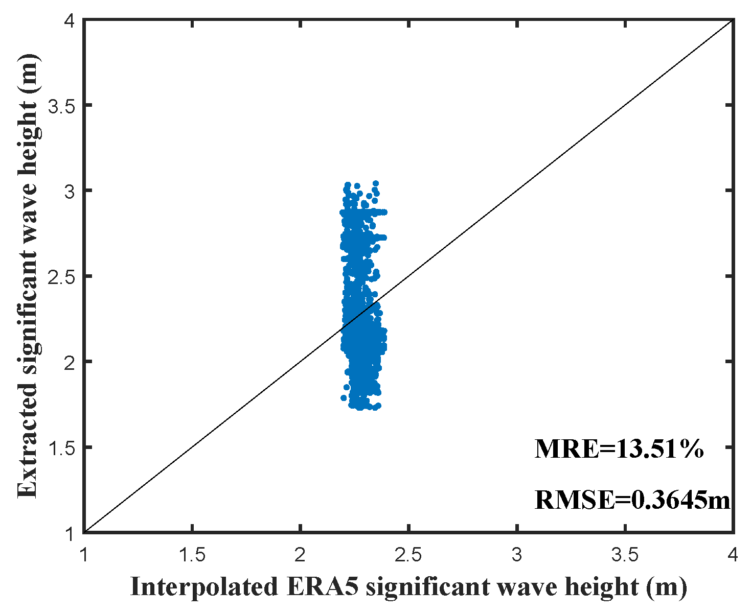The range of significant wave heights within a 20% error limit spans from about 1.6 to 2.9 m, as indicated by the green dashed lines in Figure 22, with approximately 98.82% of the extracted significant wave heights lying within this range, indicating that most of the results are close to the actual values. The scatterplots in Figure 23 further illustrate this dispersion, with the MRE and RMSE between the ERA5 and extracted values being 13.51% and 0.3645 m, respectively. Notably, the scatter points in Figure 19 and Figure 23 exhibit an approximately vertical distribution. This phenomenon is attributed to the fact that, over a short period, the actual significant wave heights within the detection area remain relatively stable and concentrated, whereas the extraction results exhibit a certain degree of fluctuation.

In addition, the significant wave heights extracted from shipborne HFSWR data after averaging represent the values at the midpoint of each interval. For example, the significant wave heights extracted from the first data group (20:35–20:45) are assigned to 20:40. Figure 24 compares the extracted significant wave heights at the buoy’s nearest location with buoy measurements during the experiment, yielding an MRE of 11.81% and an RMSE of 0.3244 m. Through interpolation, the ERA5 significant wave height at the buoy’s location at 21:00 is 2.2307 m, indicating strong agreement between the two datasets. This demonstrates the accuracy of the model-driven ERA5 data, which can thus accurately reflect real-time conditions.

4.3. Feasibility Analysis of the Method Under Different Sea Conditions

The two experiments were conducted under varying sea conditions with fully developed wind seas. The accuracy of the extracted significant wave heights is considered to be acceptable, indicating the initial feasibility of the proposed method for extracting significant wave heights from the first-order Bragg peaks of shipborne HFSWR with a single antenna. However, shipborne HFSWR currently lacks measured data under developing wind seas. Further verification is required to assess how variations in the nondimensional fetch under developing wind seas affect practical applications to confirm the feasibility of the proposed method under such conditions.

5. Discussion

The analysis of field experimental data is promising for the extraction method, although some scatter is observed in the extracted values relative to the reference data. The observed scatter can be attributed to several factors and assumptions. These factors and assumptions, as well as the comparison of the extraction method with other shipborne wave height measurement techniques, will be discussed as follows:

During navigation, six oscillatory motions introduce modulations to the Doppler spectrum, leading to additional peaks superimposed on the first-order Bragg peaks [50,51]. Although least-squares fitting is used to mitigate this effect, its influence persists in the extraction of spreading parameters and reduces the accuracy of wind speed and significant wave height estimations.

The integrated compensation relies on the assumption of a uniform radial current, which may have limited applicability in complex ocean environments. More accurate current data could enhance the accuracy of the extracted significant wave height.

Section 2.1 states that the ideal receiving antenna should be a directional sensor with a single-side-looking system, whereas the omnidirectional antenna used in the experiments results in left–right ambiguity. Fortunately, coastal navigation helps to mitigate the impact of this ambiguity on the collected data. In the future, designing a suitable antenna could facilitate single-side reception.

Wind direction inversion is performed under usual wind conditions, assuming gradual variations in sea cells at adjacent azimuths and the same range. In the presence of extreme wind variations, the inversion process may fail, leading to incorrect values for the inverted wind direction and spreading parameter. Due to the indirect nature of the extraction method, such errors could result in significant deviations between the extracted significant wave heights and the true values. Therefore, the extraction method is not recommended under extreme wind variations.

Waves include locally generated wind waves and swells propagating over long distances [52]. Short wind waves generate first-order Bragg peaks at mid- and upper-range high frequencies, aligning with the wind direction. However, at lower radar frequencies and specific sea states, swells can also induce first-order Bragg peaks, introducing errors in wind and wave field extraction. Increasing the radar frequency can mitigate this issue. However, for shipborne HFSWR, wind and wave field extraction can only be performed when the positive and negative first-order Bragg peaks do not overlap. Therefore, according to Equation (4), the radar frequency can be expressed as

$$f_0\le {\displaystyle \frac{cg}{4\pi v^2}}$$

(31)

Future work should investigate how to balance selecting the frequency of shipborne HFSWR to reduce the influence of swells in the extraction of wind wave field information. Furthermore, Equation (16) describes the relationship between significant wave height and wind speed under the wind-generated sea. Therefore, the method is mainly applicable when wind waves are the dominant component. In the future, detailed analysis and modelling of swells will be conducted to refine the significant wave height extraction method and expand its applicability.

The extraction method we propose offers a wider measurement range than shipborne wave recorders [53], requires no additional hardware or software support, and has lower maintenance costs. While it has lower accuracy compared to shipborne X-band radar [54], it provides a broader detection range and is unaffected by weather conditions. In contrast to a shipborne Global Navigation Satellite System (GNSS) [55,56], it has a smaller detection range but offers higher accuracy and avoids satellite coverage limitations. Compared to convolutional neural networks using shipborne radar data [57,58], it has lower accuracy but eliminates the need for prior data training. Therefore, this method presents several advantages over the existing shipborne measurement technologies.

6. Conclusions

This paper presents a method for extracting significant wave height from the spreading first-order Bragg peaks of shipborne HFSWR using a single antenna, addressing a critical gap in wave field extraction technology for shipborne systems. The proposed method is theoretically applicable not only to fully developed wind seas but also to developing wind seas under specific nondimensional fetch conditions. It is not affected by antenna pattern distortions caused by the shipborne structure. Furthermore, the method fundamentally differs from onshore extraction techniques as significant wave heights are indirectly derived through the progressive inversion of wind directions, spreading parameters, and wind speeds, thereby enabling the simultaneous extraction of large-scale wind and wave field information.

Wind field inversion relies on a modified cardioid directional factor model, the adjacent azimuths’ positive and negative first-order Bragg peaks, and the relationship between the spreading parameter and wind speed. Significant wave height is extracted by reversing the wind speed inversion method of onshore systems to serve wind speed as the input and replacing the spectral peak frequency in the SMB relationship to link significant wave height only with wind speed. In addition, due to the indirect nature of the extraction method, a preprocessing step is introduced before wind speed inversion. This step mitigates the influence of outliers in the spreading parameters caused by external noise and discretization errors, thereby improving accuracy.

Simulations investigate the effects of current, nondimensional fetch, noise, and shipborne structure on extraction accuracy. Integrated compensation addresses the frequency shift induced by the current, and the results confirm that antenna pattern distortions do not influence extraction accuracy. The proposed method successfully extracts significant wave heights from field experiment data collected under fully developed wind seas, with the results aligning well with ERA5 data and buoy measurements. The MRE and RMSE values are consistent with the expectations, thus validating the feasibility of the method. However, the feasibility of the method under developing wind seas requires further validation through additional experimental data collection under such conditions.

Finally, the effects of six oscillatory motions, current compensation, antenna directionality, and swells on the accuracy of significant wave height extraction are discussed. In conclusion, the proposed method demonstrates considerable potential for extracting significant wave height using shipborne HFSWR.

Future research will focus on the following aspects: (1) collecting shipborne HFSWR data under developing wind seas to assess the impact of variations in nondimensional fetch on practical applications, thereby validating the effectiveness of the extraction method; (2) long-term collection of shipborne HFSWR data under various sea conditions to further evaluate the broader applicability and robustness of the extraction method; (3) conducting detailed analyses and modeling of swells to refine the extraction method and expand its applicability; and (4) improving real-time processing or integrating AI-based methods to enhance the performance of the extraction method.

References

- Barrick, D. Accuracy of parameter extraction from sample-averaged sea-echo Doppler spectra. IEEE Trans. Antennas Propag. 1980, 28, 1–11. [Google Scholar] [CrossRef]
- Wyatt, L.R.; Ledgard, L.J.; Anderson, C.W. Maximum-Likelihood Estimation of the Directional Distribution of 0.53-Hz Ocean Waves. J. Atmos. Ocean. Technol. 1997, 14, 591–603. [Google Scholar] [CrossRef]
- Heron, M.; Rose, R. On the application of HF ocean radar to the observation of temporal and spatial changes in wind direction. IEEE J. Ocean. Eng. 1986, 11, 210–218. [Google Scholar] [CrossRef]
- Yanni, J.; Zezong, C.; Chen, Z. Research on key issues of extracting wind direction from HF surface wave radar oceanic backscatter. In Proceedings of the 2016 CIE International Conference on Radar (RADAR), Guangzhou, China, 10–13 October 2016; pp. 1–6. [Google Scholar]
- Huang, W.; Wu, S.; Gill, E.; Wen, B.; Hou, J. HF radar wave and wind measurement over the Eastern China Sea. IEEE Trans. Geosci. Remote Sens. 2002, 40, 1950–1955. [Google Scholar] [CrossRef]
- Huang, W.; Gill, E.; Wu, X.; Li, L. Measurement of Sea Surface Wind Direction Using Bistatic High-Frequency Radar. IEEE Trans. Geosci. Remote Sens. 2012, 50, 4117–4122. [Google Scholar] [CrossRef]
- Zeng, Y.; Zhou, H.; Lai, Y.; Wen, B. Wind-Direction Mapping with a Modified Wind Spreading Function by Broad-Beam High-Frequency Radar. IEEE Geosci. Remote Sens. Lett. 2018, 15, 679–683. [Google Scholar] [CrossRef]
- Stewart, R.H.; Joy, J.W. HF radio measurements of surface currents. Deep Sea Res. Oceanogr. Abstr. 1974, 21, 1039–1049. [Google Scholar] [CrossRef]
- Lipa, B.; Barrick, D. Least-squares methods for the extraction of surface currents from CODAR crossed-loop data: Application at ARSLOE. IEEE J. Ocean. Eng. 1983, 8, 226–253. [Google Scholar] [CrossRef]
- Li, L.; Wu, X. Multiple sites HFSWR ocean shallow water depth and current inversion. Acta Phys. Sin. 2014, 63, 118404. [Google Scholar]
- Lipa, B.; Nyden, B. Directional wave information from the SeaSonde. IEEE J. Ocean. Eng. 2005, 30, 221–231. [Google Scholar] [CrossRef]
- Gurgel, K.W.; Essen, H.H.; Schlick, T. An Empirical Method to Derive Ocean Waves from Second-Order Bragg Scattering: Prospects and Limitations. IEEE J. Ocean. Eng. 2006, 31, 804–811. [Google Scholar] [CrossRef]
- Roarty, H.; Evans, C.; Glenn, S.; Zhou, H. Evaluation of algorithms for wave height measurements with high frequency radar. In Proceedings of the 2015 IEEE/OES Eleveth Current, Waves and Turbulence Measurement (CWTM), St. Petersburg, FL, USA, 2–6 March 2015; pp. 1–4. [Google Scholar]
- Li, L.; Wu, X.; Long, C.; Liu, B. Regularization inversion method for extracting ocean wave spectra from HFSWR sea echo. Chin. J. Geophys. 2013, 56, 219–229. (In Chinese) [Google Scholar]
- Barrick, D. First-order theory and analysis of MF/HF/VHF scatter from the sea. IEEE Trans. Antennas Propag. 1972, 20, 2–10. [Google Scholar] [CrossRef]
- Barrick, D. Remote sensing of sea state by radar. In Proceedings of the Ocean 72—IEEE International Conference on Engineering in the Ocean Environment, Newport, RI, USA, 13–15 September 1972; pp. 186–192. [Google Scholar]
- Gill, E.W.; Walsh, J. High-frequency bistatic cross sections of the ocean surface. Radio Sci. 2001, 36, 1459–1475. [Google Scholar] [CrossRef]
- Walsh, J.; Gill, E. An analysis of the scattering of high-frequency electromagnetic radiation from rough surfaces with application to pulse radar operating in backscatter mode. Radio Sci. 2000, 35, 1337–1359. [Google Scholar] [CrossRef]
- Xie, J.; Sun, M.; Ji, Z. First-order ocean surface cross-section for shipborne HFSWR. Electron. Lett. 2013, 49, 1025–1026. [Google Scholar] [CrossRef]
- Sun, M.; Xie, J.; Ji, Z.; Cai, W. Second-Order Ocean Surface Cross Section for Shipborne HFSWR. IEEE Antennas Wirel. Propag. Lett. 2015, 14, 823–826. [Google Scholar] [CrossRef]
- Wang, Z.; Xie, J.; Ji, Z.; Quan, T. Remote sensing of surface currents with single shipborne high-frequency surface wave radar. Ocean Dyn. 2015, 66, 27–39. [Google Scholar] [CrossRef]
- Chang, G.; Li, M.; Xie, J.; Zhang, L.; Yu, C.; Ji, Y. Ocean Surface Current Measurement Using Shipborne HF Radar: Model and Analysis. IEEE J. Ocean. Eng. 2016, 41, 970–981. [Google Scholar] [CrossRef]
- Xie, J.; Yao, G.; Sun, M.; Ji, Z. Measuring Ocean Surface Wind Field Using Shipborne High-Frequency Surface Wave Radar. IEEE Trans. Geosci. Remote Sens. 2018, 56, 3383–3397. [Google Scholar] [CrossRef]
- Zhang, Y.; Wang, Y.; Ji, Y.; Li, M. Unambiguous Wind Direction Estimation Method for Shipborne HFSWR Based on Wind Direction Interval Limitation. Remote Sens. 2023, 15, 2952. [Google Scholar] [CrossRef]
- Barrick, D.E. Extraction of wave parameters from measured HF radar sea-echo Doppler spectra. Radio Sci. 1977, 12, 415–424. [Google Scholar] [CrossRef]
- Georges, T. Progress toward a practical skywave sea-state radar. IEEE Trans. Antennas Propag. 1980, 28, 751–761. [Google Scholar] [CrossRef]
- Heron, M.L.; Dexter, P.; McGann, B. Parameters of the air-sea interface by high-frequency ground-wave Doppler radar. Mar. Freshw. Res. 1985, 36, 655–670. [Google Scholar] [CrossRef]
- Wyatt, L.R. Limits to the Inversion of HF Radar Backscatter for Ocean Wave Measurement. J. Atmos. Ocean. Technol. 2000, 17, 1651–1666. [Google Scholar] [CrossRef]
- Deng, M.; Zhao, C.; Chen, Z.; Ding, F.; Wang, T. Wave Height and Wave Period Measurements Using Small-Aperture HF Radar. IEEE Trans. Geosci. Remote Sens. 2022, 60, 1–12. [Google Scholar] [CrossRef]
- Barrick, D.; Headrick, J.; Bogle, R.; Crombie, D. Sea backscatter at HF: Interpretation and utilization of the echo. Proc. IEEE 1974, 62, 673–680. [Google Scholar] [CrossRef]
- Zhou, H.; Wen, B. Wave Height Extraction from the First-Order Bragg Peaks in High-Frequency Radars. IEEE Geosci. Remote Sens. Lett. 2015, 12, 2296–2300. [Google Scholar] [CrossRef]
- Jin, L.; Wen, B.; Zhou, H. A New Method of Wave Mapping with HF Radar. Int. J. Antennas Propag. 2016, 2016, 4135404. [Google Scholar] [CrossRef]
- Tian, Y.; Tian, Z.; Zhao, J.; Wen, B.; Huang, W. Wave Height Field Extraction from First-Order Doppler Spectra of a Dual-Frequency Wide-Beam High-Frequency Surface Wave Radar. IEEE Trans. Geosci. Remote Sens. 2020, 58, 1017–1029. [Google Scholar] [CrossRef]
- Tian, Z.; Tian, Y.; Wen, B.; Wang, S.; Zhao, J.; Huang, W.; Gill, E.W. Wave-Height Mapping from Second-Order Harmonic Peaks of Wide-Beam HF Radar Backscatter Spectra. IEEE Trans. Geosci. Remote Sens. 2020, 58, 925–937. [Google Scholar] [CrossRef]
- Tian, Z.; Tian, Y.; Wen, B.; Zhao, J. Wave-Height Map Extraction from Compact HF Surface-Wave Radar Network. IEEE Geosci. Remote Sens. Lett. 2021, 18, 77–81. [Google Scholar] [CrossRef]
- Tyler, G.L.; Teague, C.C.; Stewart, R.H.; Peterson, A.; Joy, J.W. Wave directional spectra from synthetic aperture observations of radio scatter. Deep Sea Res. Oceanogr. Abstr. 1974, 21, 989–1016. [Google Scholar] [CrossRef]
- Barton, D.K. Modern Radar System Analysis; Artech House Publishers: Norwood, MA, USA, 1988; 607p. [Google Scholar]
- Long, A.; Trizna, D. Mapping of North Atlantic winds by HF radar sea backscatter interpretation. IEEE Trans. Antennas Propag. 1973, 21, 680–685. [Google Scholar] [CrossRef]
- Barrick, D.; Snider, J. The statistics of HF sea-echo Doppler spectra. IEEE Trans. Antennas Propag. 1977, 25, 19–28. [Google Scholar] [CrossRef]
- Barrick, D.E.; Lipa, B.J. A Compact Transportable HF Radar System for Directional Coastal Wave Field Measurements. In Ocean Wave Climate; Earle, M.D., Malahoff, A., Eds.; Springer: Boston, MA, USA, 1979; pp. 153–201. [Google Scholar]
- Wu, J. Wind-stress coefficients over sea surface from breeze to hurricane. J. Geophys. Res. 1982, 87, 9704–9706. [Google Scholar] [CrossRef]
- Dexter, P.E.; Theodoridis, S. Surface wind speed extraction from HF sky wave radar Doppler spectra. Radio Sci. 1982, 17, 643–652. [Google Scholar] [CrossRef]
- Bretschneider, C.L. REVISED WAVE FORECASTING RELATIONSHIPS. Coast. Eng. Proc. 1951, 1, 1. [Google Scholar] [CrossRef]
- Pierson, W.J.; Moskowitz, L. A proposed spectral form for fully developed wind seas based on the similarity theory of S. A. Kitaigorodskii. J. Geophys. Res. Atmos. 1964, 69, 5181–5190. [Google Scholar] [CrossRef]
- Pierson, W.J. The interpretation of wave spectrums in terms of the wind profile instead of the wind measured at a constant height. J. Geophys. Res. Atmos. 1964, 69, 5191–5203. [Google Scholar] [CrossRef]
- Howell, R.; Walsh, J. Measurement of ocean wave spectra using narrow-beam HE radar. IEEE J. Ocean. Eng. 1993, 18, 296–305. [Google Scholar] [CrossRef]
- Hasselmann, K.; Barnett, T.; Bouws, E.; Carlson, H.; Cartwright, D.; Enke, K.; Ewing, J.; Gienapp, H.; Hasselmann, D.; Kruseman, P.; et al. Measurements of wind-wave growth and swell decay during the Joint North Sea Wave Project (JONSWAP). Deut. Hydrogr. Z. 1973, 8, 1–95. [Google Scholar]
- Hersbach, H.; Bell, B.; Berrisford, P.; Biavati, G.; Horányi, A.; Muñoz Sabater, J.; Nicolas, J.; Peubey, C.; Radu, R.; Rozum, I.; et al. ERA5 Hourly Data on Single Levels from 1940 to Present. 2023. Available online: https://cds.climate.copernicus.eu/datasets/reanalysis-era5-single-levels?tab=overview (accessed on 6 September 2024).
- Bartier, P.M.; Keller, C. Multivariate interpolation to incorporate thematic surface data using inverse distance weighting (IDW). Comput. Geosci. 1996, 22, 795–799. [Google Scholar] [CrossRef]
- Yao, G.; Xie, J.; Huang, W. First-order ocean surface cross-section for shipborne HFSWR incorporating a horizontal oscillation motion model. IET Radar Sonar Navig. 2018, 12, 973–978. [Google Scholar] [CrossRef]
- Yao, G.; Xie, J.; Ji, Z.; Sun, M. The first-order ocean surface cross section for shipborne HFSWR with rotation motion. In Proceedings of the 2017 IEEE Radar Conference (RadarConf), Seattle, WA, USA, 8–12 May 2017; pp. 0447–0450. [Google Scholar]
- Lipa, B.; Barrick, D. Methods for the extraction of long-period ocean wave parameters from narrow beam HF radar sea echo. Radio Sci. 2016, 15, 843–853. [Google Scholar] [CrossRef]
- Clayson, C.H. Digital signal processing in a new shipborne wave recorder. In Proceedings of the Seventh International Conference on Electronic Engineering in Oceanography, 1997 ‘Technology Transfer from Research to Industry’, Southampton, UK, 23–25 June 1997. [Google Scholar]
- Liu, X.; Huang, W.; Gill, E.W. Wave Height Estimation from Shipborne X-Band Nautical Radar Images. J. Sens. 2016, 2016, 1078053. [Google Scholar] [CrossRef]
- Wang, F.; Yang, D.; Wang, J.; Xing, J.; Yu, Y. Shipborne GNSS reflectometry for monitoring along-track significant wave height and wind speed. Ocean Eng. 2023, 281, 114935. [Google Scholar] [CrossRef]
- Bai, Z.; Li, Y.; He, Q.; Yuan, J. Retrieval of significant wave height based on multi-channel fusion using shipborne GPS/BDS reflectometry. Measurement 2025, 243, 116416. [Google Scholar] [CrossRef]
- Wang, F.; Chu, X.; Zhang, B. Significant wave height estimation from shipborne marine radar data using convolutional and self-attention network. Ocean Dyn. 2024, 74, 97–112. [Google Scholar] [CrossRef]
- Chen, X.; Huang, W. Spatial–Temporal Convolutional Gated Recurrent Unit Network for Significant Wave Height Estimation from Shipborne Marine Radar Data. IEEE Trans. Geosci. Remote Sens. 2022, 60, 4201711. [Google Scholar] [CrossRef]
Figure 1.
First-order Bragg frequencies of shipborne HFSWR with a single receiving antenna.
Figure 2.
Shipborne HFSWR with a single receiving antenna.
Figure 3.
Comparison of significant wave height results under fully developed wind seas.
Figure 4.
Comparison of significant wave height results under developing wind seas.
Figure 5.
The relative error ratio curve of the significant wave height extraction.
Figure 6.
Sea cell legend: green indicates boundary sea cells and blue indicates internal sea cells.
Figure 7.
The complete process of extracting the significant wave height from the spreading first-order Bragg peaks of shipborne HFSWR with a single antenna.
Figure 8.
Simulation results of spreading first-order Bragg peaks for shipborne HFSWR with a single antenna: (a) Condition 1. (b) Condition 2. (c) Condition 3. (d) Condition 4. (e) Condition 5. (f) Condition 6. (g) Condition 7. (h) Condition 8.
Figure 9.
Wind and wave field extraction results: (a–e) Condition 1. (f–j) Condition 3. (k–o) Condition 5. (p–t) Condition 7.
Figure 10.
Spreading first-order Bragg peaks of shipborne HFSWR with a single antenna before and after compensation: (a) before; (b) after.
Figure 11.
Relative errors of the significant wave heights caused by nondimensional fetch .
Figure 12.
The spreading first-order Bragg peaks of shipborne HFSWR with a single antenna (with and without noise).
Figure 13.
Relative errors of significant wave heights caused by external noise.
Figure 14.
Transmitting and receiving antenna patterns affected by shipborne structure: (a) transmitting; (b) receiving.
Figure 15.
Spreading first-order Bragg peaks and significant wave height extraction: (a) the spreading first-order Bragg peaks; (b) the significant wave height extraction results.
Figure 16.
Relative errors of significant wave heights caused by current, nondimensional fetch, and external noise.
Figure 17.
The extracted wind and wave field information maps of Experiment 1: (a) wind direction; (b) spreading parameter; (c) wind speed; (d) significant wave height.
Figure 18.
The interpolated ERA5 significant wave height map of Experiment 1.
Figure 19.
Scatterplots comparing the extracted significant wave heights and the interpolated ERA5 significant wave heights of Experiment 1.
Figure 20.
The extracted wind and wave field information maps of Experiment 2: (a) wind direction; (b) spreading parameter; (c) wind speed; (d) significant wave height.
Figure 21.
The interpolated ERA5 significant wave height map of Experiment 2.
Figure 22.
The histograms of the interpolated ERA5 and extracted significant wave heights of Experiment 2: (a) the interpolated ERA5; (b) the shipborne HFSWR extraction.
Figure 23.
Scatterplots comparing the extracted significant wave heights and the interpolated ERA5 significant wave heights of Experiment 2.
Figure 24.
Extracted significant wave heights and buoy measurements of Experiment 2.