Estimating Aboveground Biomass and Carbon Sequestration in Afforestation Areas Using Optical/SAR Data Fusion and Machine Learning

Abstract

The growing population and the impacts of climate change present a major challenge to forests, which play a crucial role in regulating the carbon cycle. Pakistan, as a Kyoto Protocol signatory, has implemented afforestation initiatives such as the Khyber Pakhtunkhwa (KP) government’s Billion Tree Afforestation Project (BTAP). Quantifying the environmental impacts of such initiatives is very important; however, carbon pool data for BTAP plantation regions remain unavailable and are underexplored. This study aims to quantify aboveground biomass (AGB) and carbon sequestration potential (CSP) in the BTAP plantation regions using remote sensing and field data. Random sampling of 310 circular plots (17.84 m radius) provided measurements for tree height and diameter, from which AGB was calculated using allometric equations. Remote sensing data from Sentinel-1 and Sentinel-2, combined with polarization rasters and vegetation indices, were used to train and evaluate multiple regression models including multiple linear regression (MLR), support vector regression (SVR), and random forest regression (RFR). The RFR model outperformed the others (R² = 0.766) when using combined optical and radar data, yielding a mean AGB of 4.77 t/ha, carbon stock of 2.24 t/ha, and CO₂ equivalent of 10.36 t/ha. For BTAP plantations, the total biomass reached 1.19 million tons, with 2.06 million tons of CO₂ equivalent sequestered, corresponding to an annual sequestration of 0.47 tC/ha/yr and a potential of 99.18 ± 15 tC/ha. This research introduces innovative predictive models and a comprehensive carbon assessment framework for afforestation projects, providing critical insights for policymakers and climate change mitigation efforts.

1. Introduction

Climate change mitigation requires swift action, and forests play a vital role by sequestering CO₂ and storing carbon as biomass. However, burning forests releases stored carbon, undermining climate mitigation. Deforestation and land-use changes are significant drivers of greenhouse gas emissions, as deforested areas lose their ability to absorb and store CO₂, increasing the effects of global warming [1]. Forests act as global carbon sinks, protect soil and water resources, and can store large amounts of carbon [2,3,4]. Trees are primary sources of carbon storage, with coniferous wood comprising 50.8% of carbon [5]. Forests remove atmospheric carbon, storing it in wood, leaves, and soil, and is also critical to the carbon cycle and ecological balance [6,7]. They hold 70% of organic soil carbon, 80% of aboveground terrestrial carbon, and over twice the atmospheric carbon [8,9]. Global forests store approximately 650 Gt of carbon across biomass, soil, and litter [10]. Forest ecosystems account for 90% of the annual carbon exchange between the Earth’s surface and the atmosphere [11]. Additionally, forest biomass plays a key role in examining carbon cycles over large regions [12] and understanding the spatiotemporal trends in aboveground carbon (AGC) storage is essential for studying terrestrial carbon exchange mechanisms [13]. For example, the Southeast Asian forests absorb 3 Gt of CO₂ annually and store approximately 500 Mg of carbon per hectare. This demonstrates their importance in the global carbon cycle [14,15].

Pakistan joined the UNFCCC and Kyoto Protocol in 2005, committing to quantify forest carbon stocks [16]. While provincial forest departments conducted inventories, carbon stock assessments began in earnest after 2015. The FAO’s 2005 Global Forest Resources Assessment included Pakistan’s carbon stock but relied on potentially imprecise measurements derived using remote sensing data only [17]. More accurate data was produced in the 21st century, such as the stratified cluster sampling in Khyber Pakhtunkhwa (KP), which estimated a total carbon stock of 144.71 million tons, averaging 127.66 tons per hectare. The dry temperate forests held relatively high carbon content (99.41 tons per hectare) as compared to the moist temperate forests (85.04 tons per hectare) [18]. These data support the REDD+ program, with annual sequestration estimated at 6 million tons, aiding climate mitigation [19]. In Khyber Pakhtunkhwa (KP), Pakistan, the Billion Tree Afforestation Project (BTAP) has established around 198,993 hectares of young and middle-aged forests since 2014, with significant carbon sequestration potential. However, no research has evaluated its carbon stock or sequestration, leaving a critical knowledge gap.

Early assessments are essential to examine survival rates, growth performance, and natural regeneration, as external factors like fire, grazing, and grass cutting impact success. Given its climate change mitigation goal, evaluating BTAP’s carbon stock and its role in the global carbon market is crucial [20,21,22]. According to earlier research, in Buner district, Chir pine and Eucalyptus plantations were analyzed for carbon stock and biomass, with Eucalyptus primarily grown for economic purposes and harvested every 4–5 years, helping reduce pressure on natural forests [23]. This involves evaluating biophysical factors like tree count, volume, species composition, age, and growth potential [24], with forest stand age being particularly critical [25]. Carbon stocks are estimated using multiple methods including destructive methods, non-destructive methods, and remote sensing. Non-destructive techniques, such as measuring DBH and height, are widely used, while destructive methods, though accurate for developing allometric equations, are labor-intensive and limited to smaller regions [26,27]. Rapid developments in the field of remote sensing have resulted in a large volume of data which has decent spatial and temporal resolution. These data can be used for many studies, including forest AGB mapping. Remote sensing, combined with field data, provides precise and timely regional AGB estimation [28,29]. Combining optical, radar, and LiDAR data has proven effective for monitoring and measuring aboveground biomass (AGB) of forests [30,31]. It facilitates forest mapping and inventories, especially in countries where the amount of available data is very limited [32]. It enables the correlations of forest characteristics with other variables, aiding in species-level distribution mapping [33]. The use of Sentinel-1 and Sentinel-2 data has proven effective in estimating forest AGB across various biomes [34,35]. Integrating multi-source remote sensing data with statistical models, such as linear regression and machine learning, enhances AGB estimation across diverse tropical and subtropical regions [36,37].

Machine learning models can be trained using remote sensing data to provide high resolution estimation of AGB very efficiently. Previous research has explored the use of machine learning regression models, such as multiple linear regression (MLR), support vector regression (SVR), partial least square regression (PLSR), and RFR to estimate AGB in different study regions. MLR has been used to estimate forest AGB by establishing a relationship between biomass and remote sensing data. For example, Li [38] estimated forest AGB using remote sensing data and the MLR model. The study compared the results of the MLR model with other machine learning models, such as RFR and geographically weighted regression (GWR). The study concluded that the MLR and GWR models comparable results and outperformed the GWR model. The study also observed that integrating data from multiple sources produces better results as compared to using a single source of data. The PLSR model is another machine learning regression model that has been widely used to estimate AGB due to its ability to handle multicollinearity and extract useful information from high-dimensional remote sensing data. Ma et al. [39] used the PLSR model to estimate variable importance in LiDAR features which were later used to estimate biomass. The simplicity of MLR and PLSR models makes it suitable to predict AGB in different forest ecosystems; however, it assumes the relationship between the dependent variable and independent variables as linear particularly when high dimensional data are involved [40]. This can lead to poor performance in estimating the AGB. The SVR model can address this issue. The SVR model has the ability to handle the relatively complex and nonlinear relationships and can be used to estimate the AGB using remote sensing. Wang et al. [41] used Sentinel-2 imagery combined with field data and an SVR model to estimate forest AGB, achieving promising results. This demonstrates that the SVR model can better capture the nonlinear patterns in the data, which linear models may not effectively handle. The RFR model also has the ability to work with nonlinear and high dimensional data. A recent review conducted on the use of machine learning and remote sensing for forest carbon stock identified RFR as the most frequent method for forest carbon estimation. The study also mentioned that integrating data from multiple sources enhances the accuracy of biomass predictions [42]. The methods and models discussed above provide an overview of some regression models; however, there are limited studies on forest AGB biomass estimation using machine learning models utilizing remote sensing data particularly utilizing optical and SAR data together. Estimating carbon stock is vital for reforestation success and can be performed using remote sensing data leveraging machine learning regression models. In this study we aim to address the research gaps and estimate AGB utilizing remote sensing datasets. To our knowledge, there are no prior studies that assess BTAP plantations carbon stock in KP and finding the best vegetation index for mapping AGBs of plantation forests. Additionally, this study offers critical insights for resource managers and policymakers in ecosystem restoration.

The main objectives of the study were as follows: (1) to calculate the AGB/carbon stock of the study sites; (2) to quantify the carbon sequestration potential of BTAP plantations; (3) to identify the most suitable vegetation index for AGB calculation in afforestation sites; and (4) to determine the best model for mapping AGB using optical/SAR data fusion and machine learning.

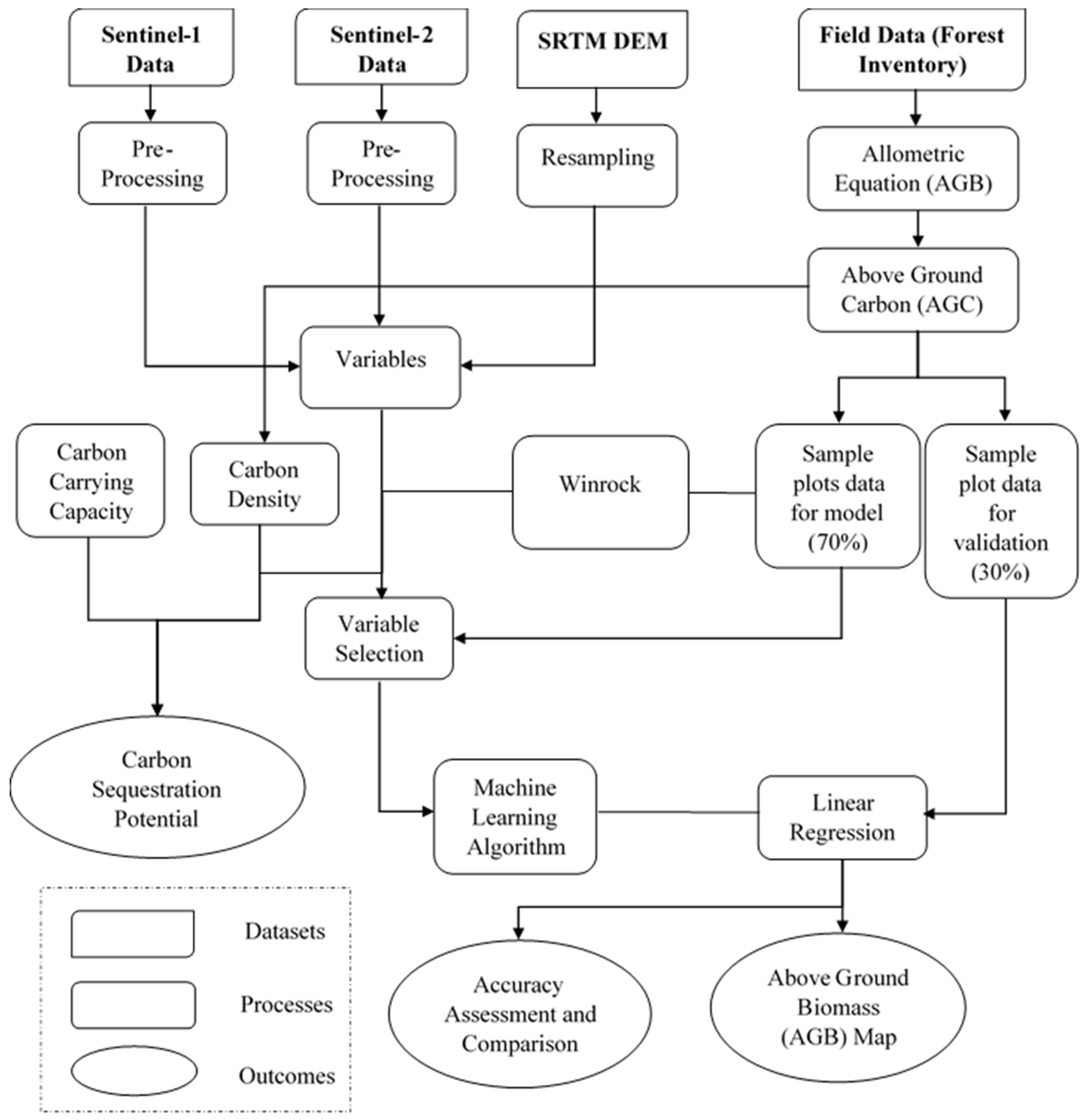
2. Materials and Methods

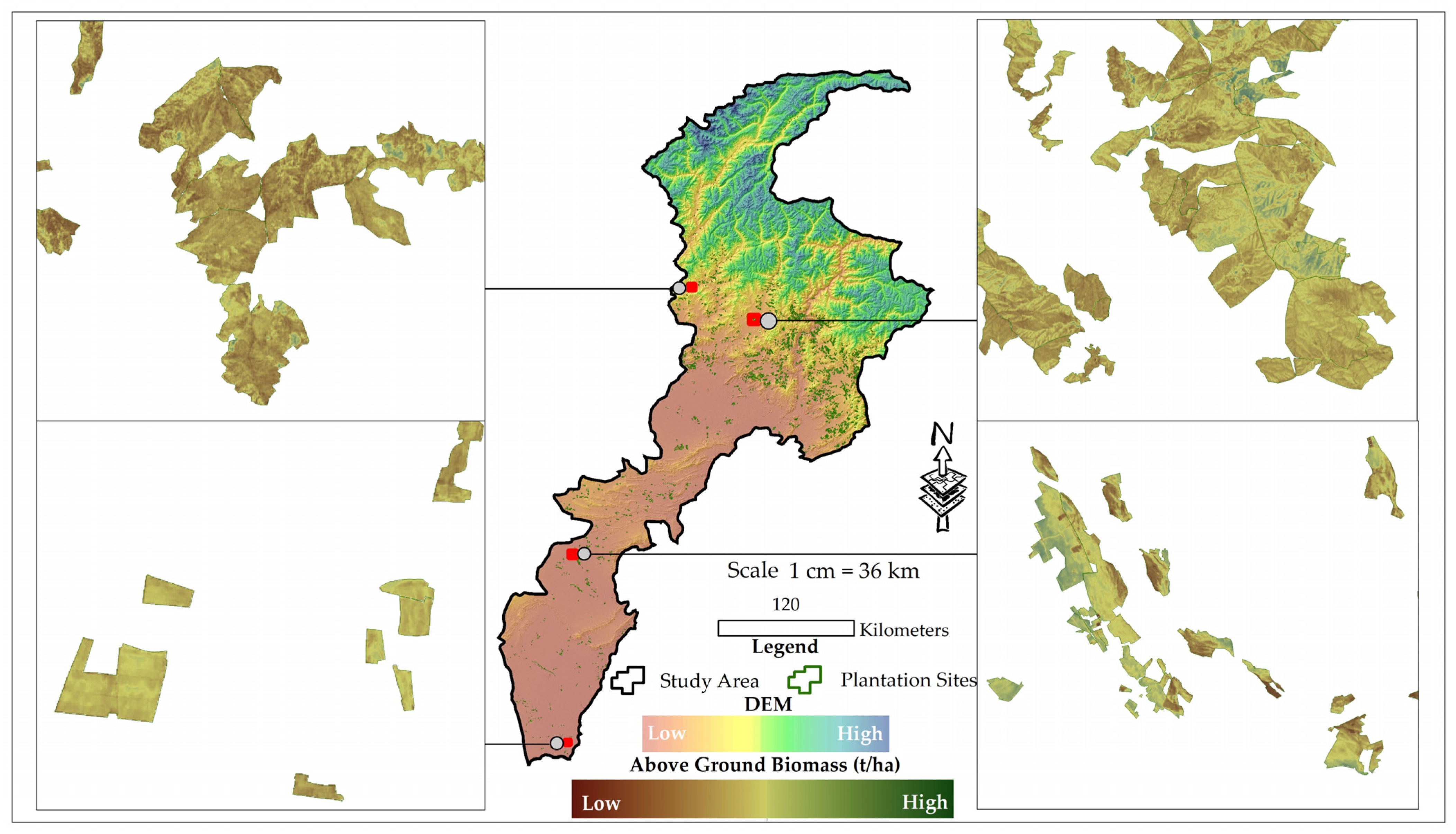
2.1. Study Area

The study sites for this study are located in the Khyber Pakhtunkhwa (KP) province, Pakistan. The study area has a total area of 7.45 million hectares, with 28 watershed and forest divisions (Figure 1). It is divided into three forest regions: Central Southern Region I (Southern Forest Circle), Northern Region II (Watershed and Hazara Forest Circle), and Northern Region III (Malakand East and West Forest Circles). KP, Pakistan’s most densely forested and smallest province by land, covers 9.36% of the country’s area. Its primary land uses are rangelands (26%), forestry (20%), and agriculture (30%). Bordered by Azad Kashmir, Punjab, Baluchistan, Gilgit Baltistan, Afghanistan, and FATA, which is presently a part of KP, KP’s elevation ranges from 200 to 6000 m. Annual precipitation averages 130–3200 mm, with temperatures ranging from −14 °C to 51 °C. Major tree species include Cedrus deodara, Abies pindrow, Pinus wallichiana, Juglans regia, and Quercus incana. Key species planted under BTAP include Eucalyptus, Robinia pseudoacacia, Acacia modesta, and Pinus roxburghii. The main crops are wheat, maize, rice, tobacco, and sugarcane. The study area’s varied climate supports diverse forest types and rich biodiversity.

2.2. Datasets

2.2.1. Field Measurements and Collection Procedure

The study focused on plantation areas in KP Province, using species and site data from KP Forest Department. Most plantations were on bare lands with minimal vegetation. Of 2511 BTAP plantation sites, 115 were sampled for comprehensive coverage. Dominant species included Eucalyptus camaldulensis, Robinia pesudoacacia, Acacia modesta, Acacia nilotica, and Pinus roxburghii. Data collection involved laying out 3–5 circular sample plots (1000 m² area, 17.84 m radius) per site, varying with plantation size, using GPS for plot coordinates and random sampling techniques. Tree diameter was measured using a diameter tape, while height measurements were taken with a Haga Altimeter and tape. Field data for the study were collected in 2019–2020 using random sampling across 310 circular plots (17.84 m radius). Measurement errors were corrected to ensure inventory accuracy [43]. Data for the plantation included GPS coordinates, species type, diameter, and height. The diameter and height were measured through a diameter tape and Haga Altimeter following field standards. A Sunnto compass was used for plot navigation, and measuring tapes were used for intra-plot and inter-plot distances [16]. The data from the field were noted using manual forms and the transferred to Excel files. The Excel data was further used to estimate biomass and carbon stock. Total carbon reserves were estimated by multiplying the average carbon stock per hectare by the plantation area.

2.2.2. Remote Sensing Data

The study used Sentinel-1 (radar) and Sentinel-2 (optical) data for analysis, leveraging their complementarity through image fusion [44]. Sentinel-1 weather independent radar capability ensured imagery during cloud cover, while Sentinel-2 spectral resolution facilitated vegetation studies. Combined, these sensors provided year-round image coverage for biomass mapping and carbon stock assessment, with SAR data demonstrating strong potential due to its correlation with AGB. Two Ground Range Detected (GRD) images, which are Sentinel-1A level 1 products with two polarization images, were used in this study. In July 2020, Sentinel-1A GRD images were obtained. Sentinel-1A provided C-band SAR data (5.405 GHz) with VV and VH polarizations, processed using SNAP 10.0.0 [45]. For despeckling, a speckle filter was used [46]. ALOS-PALSAR DEM (12.5 m) was resampled to 10 m for slope, aspect extraction and terrain correction using the relationship between the sun azimuth and elevation parameters from DEM [47]. Geographical variables, including slope and aspect, were derived from DEM data and resampled to 10 m resolution in ArcGIS Pro 3.1 Cloud-free Sentinel-2 imagery (≤10%, July 2020) of the study area was downloaded from United States Geological Survey (USGS) Earth explorer https://earthexplorer.usgs.gov (accessed on 7 September 2023). The high spatial resolution (10 m) and spectral coverage of Sentinel-2 data makes it ideal for vegetation studies, particularly with the inclusion of three red-edge bands specifically designed for vegetation monitoring. The pre-processing of Sentinel-2 data was performed using SNAP 10.0.0 and was corrected for radiometric, atmospheric, and topographic issues [48]. ArcGIS Pro 3.1 was used to resample the shortwave infrared (SWIR) and red-edge bands (20 m) to 10 m. Vegetation indices were calculated from spectral bands.

We used three vegetation indices to estimate AGB: Normalized Different Vegetation Index (NDVI), Soil Adjusted Vegetation Index (SAVI), and Red Edge Normalized Difference Vegetation Index (RENDVI) (

Table 1. Description and formula of vegetation indices and SAR data used in the study.

Sensor	Vegetation Index/SAR Bands	Formula/Parameters	Sentinel-2/Sentinel-1 Bands	Reference
	Broadband Vegetation Indices
Sentinel-2 (July–August 2020)	NDVI	$NDVI={\displaystyle \frac{NIR-RED}{NIR+RED}}$	NIR = spectral band 8 and Red = spectral band 4	[49]
Sentinel-2 (July–August 2020)	SAVI	$SAVI={\displaystyle \frac{NIR-RED}{NIR+RED+L}}\times \left(1+L\right)$	NIR = spectral band 8 and Red = spectral band 4	[50]
	Narrow Red Edge Bands VI
Sentinel-2 (July–August 2020)	RENDVI	$RENDVI={\displaystyle \frac{NIR-REDEDGE}{NIR+REDEDGE}}$	NIR = spectral band 8 and REDEDGE = spectral band 6	[51]
	Synthetic Aperture Radar (SAR) Data
Sentinel-1 (July 2020)	VV	Polarization	Vertical transmit-vertical channel	[45]
Sentinel-1 (July 2020)	VH	Polarization	Vertical transmit-horizontal channel	[45]

). NDVI and SAVI, as broadband indices, are highly sensitive to the canopy leaf area. RENDVI, a narrowband index, utilizes the red-edge spectral band (690–740 nm) instead of the red band, along with the NIR band, enhancing its applicability in vegetation studies.

2.3. Methods

In this study, we estimated the AGB using the allometric equations and field data. Additionally, we utilized vegetation indices and derived from remote sensing data and machine learning to estimate AGB. Furthermore, we estimated belowground biomass (BGB) and total biomass. These parameters were used to calculate carbon stock. We also calculated the carbon sequestration potential using the following two methods: (1) carbon carrying capacity (CCC) method, and (2) Winrock database method. The following subsection provides the methods we used for estimating these parameters. The study’s methodological framework is shown in Figure 2.

2.3.1. Allometric Equations

Diameter (D) and tree height (H) were used to calculate aboveground biomass (AGB) through allometric equations, which are regression models relating forest attributes to estimate growth parameters [52,53]. Tree diameter reflects secondary growth, while height represents primary growth. This study employed species-specific and general allometric equations developed by Ali et al., 2015 [54] and Chave et al., 2003 [55] as these equations vary by species and can be applied across forest types and bioclimates (

Table 2. List of allometric equations used in the study.

Species	Allometric Equation	Reference
General	$AGB=0.0224\left(D^2\times H\right)0.9767$	[56]
General	$AGB=0.0509\times$$\rho \left(D^2\times H\right)$	[55]
General (Coniferous)	$AGB=0.1645\left({\rho \times D}^2\times H\right)0.8586$	[56]
Pinus roxburghii (Chir)	$AGB=0.0224\left(D^2\times H\right)0.9767$	[56]
Eucalyptus camaldulensis (Eucalyptus)	$AGB=0.023\left(D^2\times H\right)0.9985$	[18]
Robinea pseudoacacia (Robinia)	$AGB=0.2586\left(D^2\times H\right)0.7786$	[54]
Cedrus deodara (Deodar)	$AGB=0.1779\left(D^2\times H\right)0.8103$	[57]
Populus deltoides (Poplar)	$AGB=0.0194\left(D^2\times H\right)0.9654$	[54]
Acacia nilotica (Kikar)	$AGB=0.0493\left(D^2\times H\right)0.9728$	[54]
Acacia modesta (Phulai)	$AGB=0.2267\left(D^2\times H\right)0.8226$	[54]
Olea ferruginea (Olea)	$AGB=7.8863+0.0556\left(D^2\times H\right)$	[54]
Dodonea viscosa (Sanatha)	$AGB=0.928{\left(D\right)}^{2.018}$	[54]

AGB = aboveground biomass, D = diameter in centimeters. H = height in meters.

).

$$BGB=AGB\times CF$$

(1)

whereas BGB is Belowground Biomass, AGB is Aboveground Biomass and CF is Conversion Factor (0.26).

AGB per plot was converted to tons/hectare by multiplying by 10 and dividing by 1000. The AGB was then multiplied by 0.47, an IPCC conversion factor, to calculate aboveground carbon (AGC), as carbon comprises about half of the total dry biomass (Equation (2)) [58]. BGB and belowground carbon (BGC) were calculated by applying a 0.26 conversion factor to AGB and AGC (Equation (1)) [59]. To calculate the total biomass AGB, and BGB, while total carbon stock (CS) was calculated as AGC and BGC. To estimate the plantation’s climate mitigation potential, CS was multiplied by 3.67, the molecular weight ratio of CO₂ to O₂, yielding CO₂ equivalents [60].

$$C=AGB\times CF$$

(2)

whereas C is carbon stock, AGB is aboveground biomass, and CF is the conversion factor (0.47).

Statistical analysis was performed using MS Excel, with outliers defined as values exceeding the mean ± 3 (standard deviation) subsequently removed. AGB was measured in tons/hectare. Carbon stock values were used to calculate carbon credits, where one credit equals one metric ton of carbon dioxide.

2.3.2. Machine Learning Models

Multiple Linear Regression Model (MLR)

MLR in machine learning is a technique that is used to establish the relationship between the dependent variable and two or more independent variables. It does so by estimating a linear equation between dependent and independent variables. It minimizes the residual sum of square (RSS) which measures the difference between observed and estimated values. MLR is one of the simplest and most interpretable regression algorithms (Equation (3)).

$$Y={\beta }_0+{\beta }_1{x}_1+{\beta }_2{x}_2+\dots +{\beta }_n{x}_n+\epsilon$$

(3)

whereas Y = Dependent variable (target), ${\beta }_0$ = Intercept (constant), $\beta ,{\beta }_2,\dots {\beta }_n$ = Coefficient for the independent variables, $x_1,x_2,\dots x_n$ = Independent variables (features) and $\epsilon$ = Error term (residual).

Support Vector Regression Model (SVR)

SVR is a classical machine learning model that is used to establish the relationship between input data and a target variable. SVR does this by determining a function that forecasts the desired values; the function is represented by a hyperplane in a higher dimensional space [61]. To minimize differences between the expected and actual values within a given tolerance margin, SVR seeks to fit this hyperplane [62]. Estimating a function, f(x), that deviates from the target, y, by no more than (epsilon) while remaining as flat as possible is the aim of SVR (Equation (4)).

$$f\left(x\right)=\left(w,x\right)+b$$

(4)

whereas w = Weight vector, x = Input features and b = Bias term. To accomplish this, the optimization issue is described in Equation (5):

$$Minimize:\left({\displaystyle \frac{1}{2}}\right){‖w‖}^2$$

(5)

$$ST:\left|{y\_}_i-f\left({x\_}_i\right)\right|\le \epsilon +{\xi }_i,{\xi }_{i^{*}}\ge 0$$

(6)

where ST in Equation (6) means subject to and ${\xi }_i$ and ${\xi }_{i^{*}}$ are slack variables to handle the data points outside the (epsilon)-tube, confirming that the optimization issue can be resolved.

Random Forest Regression (RFR)

RFR is a classical machine learning model that is based on decision trees and offers higher accuracy and robustness compared to individual trees. It provides variable importance, resists data reduction, and estimates generalization error during forest building [63]. The RFR model works by creating an ensemble of decision trees. During training, each decision tree is trained using a subset of features. This splitting is called bootstrap aggregation or bagging. The final output is calculated by averaging the output of all the individual trees. Due to this, the RFR model is sometimes highly accurate compared to other classical machine learning models and can handle the non-linearity in the input data very efficiently. Due to the bagging mechanism, the RFR model is not dependent on a specific number of features or samples which makes it very robust and less prone to overfitting.

2.4. Data Preprocessing and Model Training and Evaluation

To generate the input data for machine learning models, data collected from the field and features derived from remote sensing imagery were combined with unique plot identification. The derived features included variables such as NDVI, RENDVI, SAVI and SAR variables. The samples were split into training and testing datasets with 70% of data used for training the models while 30% of the data were utilized to independently evaluate the accuracy of the models. Figure 3 illustrates the distribution and frequency of AGB data used for model testing and training. To train the machine learning models, python library Scikit-learn was used in Jupyter Notebook Version 7.3 which is an open-source system to use python libraries. To compare the accuracy of the models, we used R², RMSE and RRMSE (%). The mathematical equations of R², RMSE, and RRMSE (%) are provided as follows:

$$R^2=1-{\displaystyle \frac{\sum _{i=1}^n{{\widehat{(y}}_i-y_i)}^2}{\sum _{i=1}^n{{\widehat{(y}}_i-{\overline{y}}_i)}^2}}$$

(7)

$$RMSE=\sqrt{{\displaystyle \frac{\sum _{i=1}^n{{\widehat{(y}}_i-y_i)}^2}{n}}}$$

(8)

$$RRMSE\%={\displaystyle \frac{RMSE}{\overline{y}}}\times 100$$

(9)

where $n$ is the number of samples, ${\widehat{y}}_i$ is the estimated AGB, and $y_i$ is AGB measured from field data. $\overline{y}$ is the average of all observed values of AGB.

2.5. Carbon Sequestration Potential Calculation

To estimate the carbon sequestration potential (CSP) the following two methods were used: (1) carbon carrying capacity (CCC), and (2) the Winrock database methods. These methods are very effective in estimating CSP. As forests grow, their carbon storage potential increases rapidly, making them effective carbon sinks. In old-growth forests, carbon storage stabilizes as carbon exchange with the atmosphere approaches equilibrium, leading to a carbon-neutral stage [64]. These forests can serve as benchmarks for carbon carrying capacity (CCC) in similar climatic conditions. However, assessing carbon sequestration potential (CSP) is challenging due to limited data on old-growth forests [65]. CSP can be estimated using Equation (10) by comparing the carbon densities of old-growth and current forests [66].

$$CSP=CCC-CD$$

(10)

whereas CCC is carbon carrying capacity while CD is carbon density.

The potential of fast-growing species to sequester carbon was assessed using the Winrock database [67], developed by Winrock International and IUCN to analyze emissions from deforestation, forest degradation, and carbon removal in Forest Landscape Restoration (FLR) projects. Required inputs included species per hectare and year of plantation. Species per hectare data were collected from the field, while plantation year data came from the KP Forest Department. Proportions of species in sample plots (radius 17.84 m) were calculated in Excel and converted into species per hectare.

3. Results

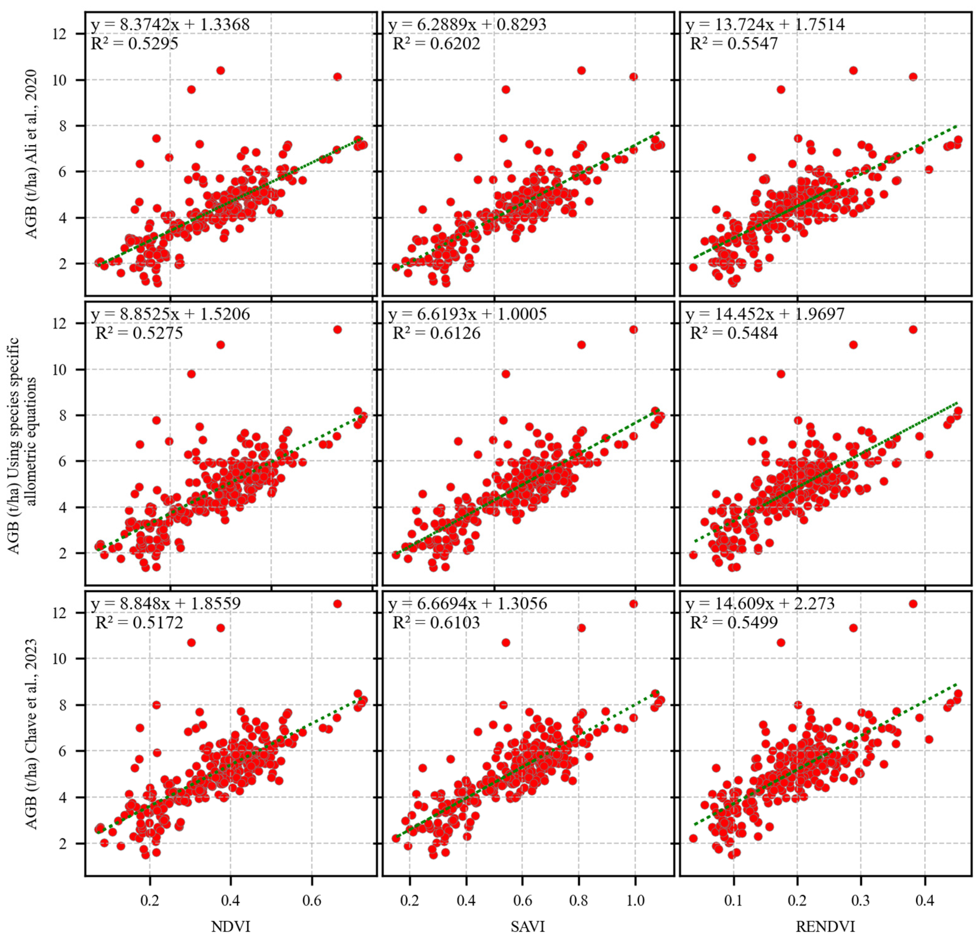
3.1. The Results of Aboveground Biomass and Carbon Stock Using Allometric Equations

In the study area, forest area has increased over the past decade due to the BTAP plantation, as indicated by land use land cover classification [68]. The AGB/AGC also increased from 2014 to 2020 due to the BTAP plantation. Major planted species included Eucalyptus, Robinia pseudoacacia, and Pinus roxburghii. Field data from 310 plots showed that AGB ranged from 12.38 t/ha to 1.15 t/ha (mean: 4.77 t/ha, 4.41 t/ha, 5.10 t/ha), while AGC ranged from 5.82 t/ha to 0.54 t/ha (mean: 2.24 t/ha, 2.07 t/ha, 2.40 t/ha) as shown in

Table 3. Descriptive summary statistics of biomass, carbon stock and CO₂ e using each type of allometric equations.

Statistics	AGB (t/ha)			BGB (t/ha)			Total Biomass (t/ha)			AGC (t/ha)			BGC (t/ha)			Total Carbon (t/ha)			CO2 e (t/ha)
	Using Species Wise	Using [54]	Using [55]	Using Species Wise	Using [54]	Using [55]	Using Species Wise	Using [54]	Using [55]	Using Species Wise	Using [54]	Using [55]	Using Species Wise	Using [54]	Using [55]	Using Species Wise	Using [54]	Using [55]	Using Species Wise	Using [54]	Using [55]
Sum	1448.51	1339.34	1549.93	376.61	348.23	402.98	1825.12	1687.57	1952.91	680.79	629.49	728.47	177.01	163.67	189.40	857.80	793.16	917.87	3139.57	2902.96	3359.40
Mean	4.77	4.41	5.10	1.24	1.15	1.33	6.00	5.55	6.42	2.24	2.07	2.40	0.58	0.54	0.62	2.82	2.61	3.02	10.33	9.55	11.05
St. Dev	1.48	1.39	1.49	0.38	0.36	0.39	1.86	1.76	1.88	0.69	0.65	0.70	0.18	0.17	0.18	0.87	0.82	0.88	3.19	3.02	3.23
Min	1.35	1.15	1.49	0.35	0.30	0.39	1.70	1.45	1.87	0.64	0.54	0.70	0.17	0.14	0.18	0.80	0.68	0.88	2.93	2.49	3.22
Max	11.73	10.39	12.38	3.05	2.70	3.22	14.78	13.09	15.60	5.52	4.88	5.82	1.43	1.27	1.51	6.95	6.15	7.33	25.43	22.52	26.84
Range	10.38	9.24	10.9	2.698	2.40	2.83	13.079	11.64	13.73	4.88	4.34	5.12	1.27	1.13	1.33	6.15	5.47	6.45	22.49	20.03	23.62
Skewness	0.52	0.46	0.56	0.52	0.46	0.56	0.52	0.46	0.56	0.52	0.46	0.56	0.52	0.46	0.56	0.52	0.46	0.56	0.52	0.46	0.56

CO₂ e = Carbon dioxide equivalent.

. Total BTAP plantation AGB and AGC were 0.949–1.015 Mt and 0.412–0.478 Mt, respectively. CO₂ e values varied from 2.49 t/ha to 26.84 t/ha, with a mean of 9.55–11.05 t/ha. The annual mean carbon sequestration from 2015 to 2020 was 0.47 t/ha/yr, with a total CO₂ e of 1.9–2.2 Mt. The carbon sequestration potential was 99.18 ± 15 t/ha, yielding 2.06 million carbon credits by 2020. Biomass estimates varied across equations, with Chave, Condit, Lao, Caspersen, Foster and Hubbell [55] giving the highest values, and Ali et al. [56] the lowest (2.61–3.02 t/ha).

3.2. Belowground Biomass, Total Biomass, Total Carbon Stock and Anuual Sequestrations

BGB ranged from 3.22 t/ha to 0.30 t/ha (mean: 1.24 t/ha, 1.15 t/ha, 1.33 t/ha), while BGC ranged from 1.51 t/ha to 0.14 t/ha (mean: 0.58 t/ha, 0.54 t/ha, 0.62 t/ha). Total BGB was 0.229–0.265 Mt, and total BGC was 0.108–0.123 Mt (Table 3). Biomass ranged from 15.60 t/ha to 1.45 t/ha (mean: 6.00 t/ha, 5.55 t/ha, 6.42 t/ha), while carbon ranged from 7.33 t/ha to 0.68 t/ha (mean: 2.82 t/ha, 2.61 t/ha, 3.02 t/ha) across equations. Total biomass (AGB + BGB) was 1.104–1.278 Mt, and total carbon (AGC + BGC) was 0.519–0.6 Mt. From 2015 to 2020, plantation forests covering 198,993 hectares showed an annual carbon stock increase of 0.47 t/ha.

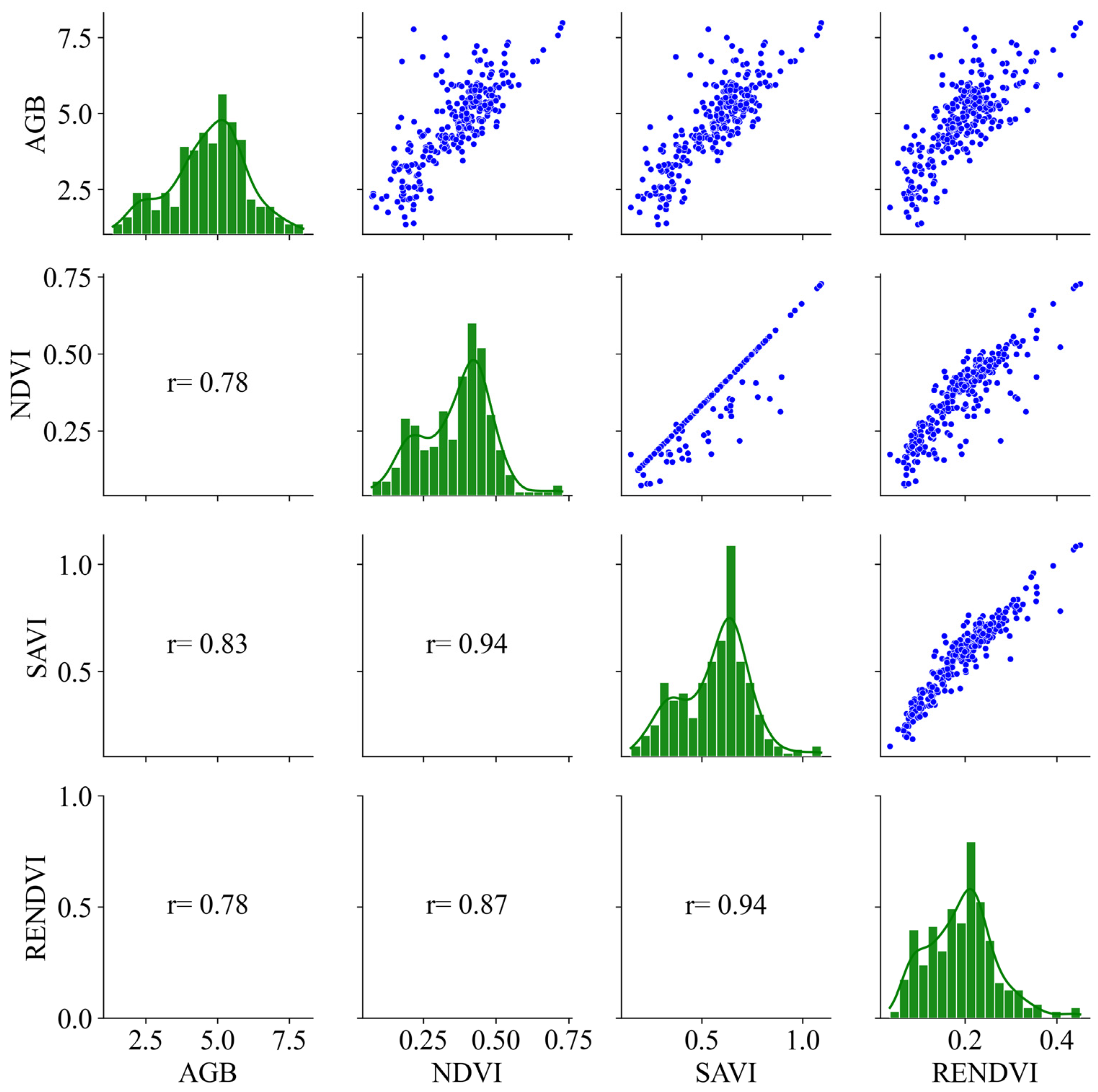
3.3. Correlation Analysis of AGB and Remote Sensing Vegetation Indices

Vegetation indices vary in sensitivity to biomass and groundcover due to factors like topography, soil reflectance, and internal canopy signal scattering [50]. Three vegetation indices were analyzed for their correlation with biomass estimates. Among them, the SAVI showed the stronger correlation (R = 0.83, p ≤ 0.01). Similarly, RENDVI and NDVI demonstrated a correlation value (R = 0.78) with AGB demonstrating a similar relation with AGB for this study (Figure 4). Vegetation indices rely on NIR and RED bands of the electromagnetic spectrum; hence, a dense and healthy vegetation will lead to higher reflectance in NIR band [69]. Vegetation indices using the red-edge band (λ = 740 nm) reduce saturation effects compared to the red band (λ = 665 nm), which has higher absorptivity and sensitivity. Since red-edge band is not very sensitive to the chlorophyll content, it minimizes the saturation effects [70].

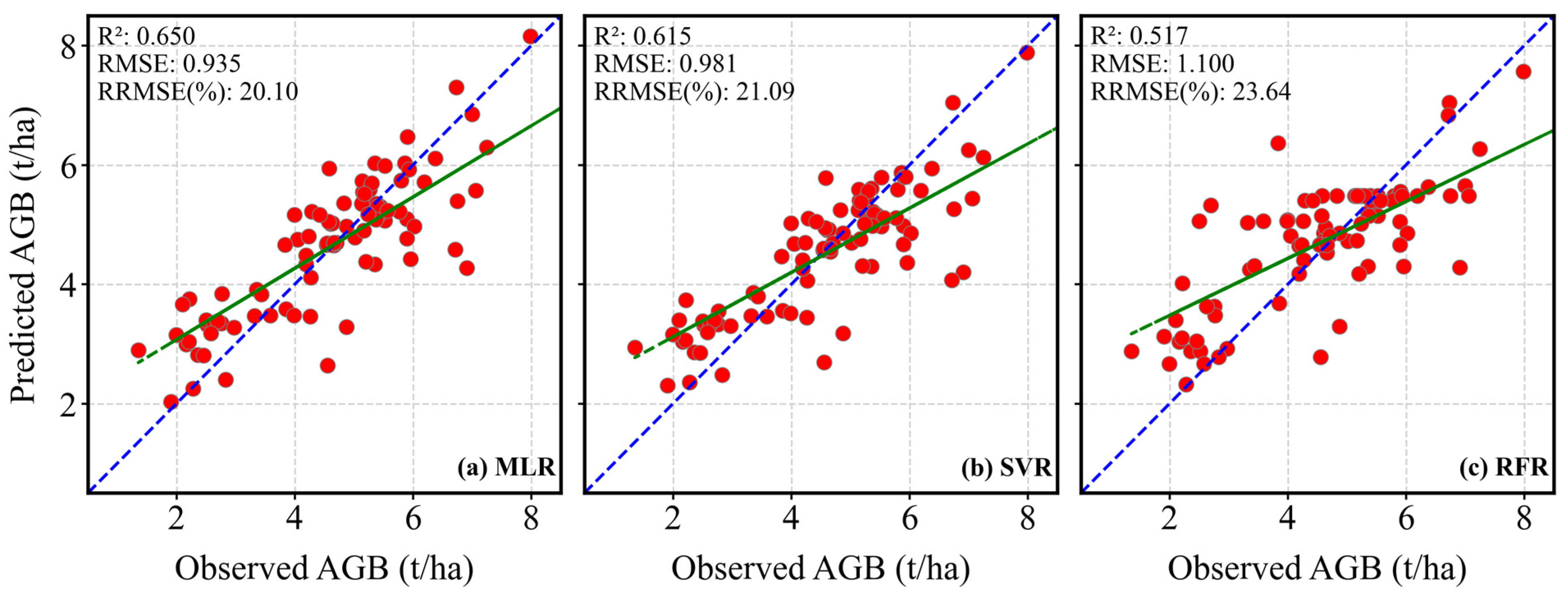
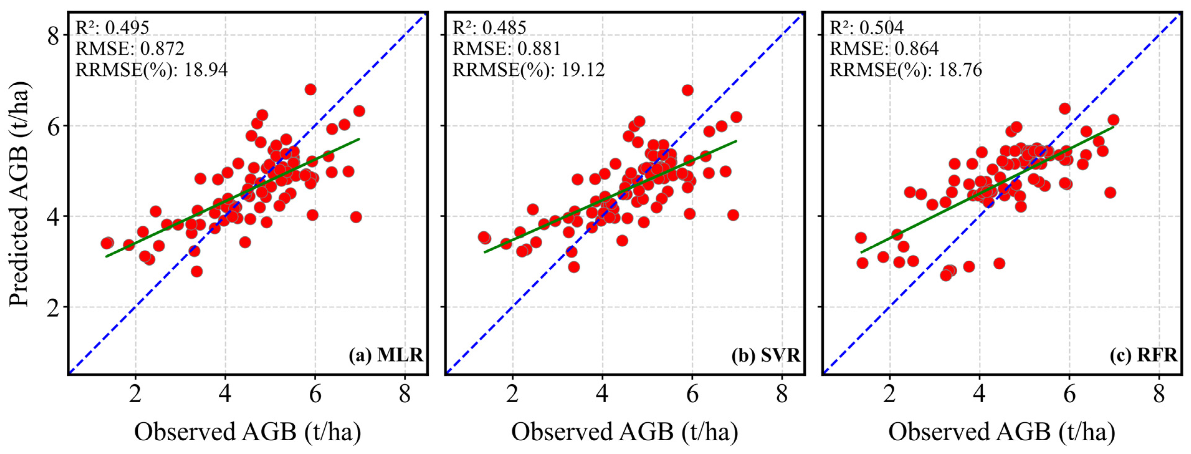
3.4. Evaluation of Simple Linear Regression and Machine Learning for AGB Estimation

Our results demonstrate that Sentinel-2 vegetation indices significantly correlate with AGB, with SAVI performing best (R² = 0.62, RMSE = 1.09 t/ha) in a simple linear regression (SLR) model using field biomass data (Figure 5). Figure 6 illustrates the scatterplot between vegetation indices and AGB values. The effectiveness of SAVI is due to its soil-adjustment capability, making it ideal in plantation forests for sparse vegetation and semi-arid regions, where soil exposure is prominent thus allowing it to capture biomass more accurately, thereby making it the most suitable vegetation index in such conditions. RENDVI provides a balance between vegetation density sensitivity and soil adjustment, performing well in sparse plantations; however, it is less effective compared SAVI in low-density areas. NDVI, with a lower R², struggles in sparse conditions due to soil interference, reducing its biomass estimation accuracy. Based on the highest correlation value SAVI was used to fit the SLR model. The predicted AGB values of the SLR model using SAVI ranged from 2.05–8.51 t/ha.

In machine learning models, the RFR model achieved the highest accuracy for AGB estimation with an R² value of 0.766, outperforming linear regression (0.62), MLR (0.756), and SVR (0.755) (

Table 4. Accuracy of linear regression model and random forest model.

Model	R2	RMSE (t/ha)	RRMSE%	p-Value
LR	0.62	1.09	23.29	p ≤ 0.01
SVR	0.755	0.618	13.22	p ≤ 0.01
MLR	0.756	0.617	13.18	p ≤ 0.01
RF	0.766	0.604	12.91	p ≤ 0.01

). The RFR model achieved the lowest RMSE and RRMSE% of 0.604 t/ha and 12.91 compared to 1.09 t/ha in the linear regression model (Figure 7). Although the RFR model performed better than the other two machine learning models, the difference in results was not significant. This suggests that MLR can perform equally well compared to SVR and RFR in estimating AGB in forests. While the performance of the machine learning models was comparable, their results were superior to those of simple linear regression, as ML models utilize multiple variables for training. The variables derived from combined optical and radar data provided greater accuracy than those from a single source. The results of this study align with other studies conducted on AGB estimation using remote sensing and machine learning. For example, Shen et al., 2016 [31] also found RF effective when using time series Landsat data images for AGB estimation, with an R² of 0.51 and RMSE of 39.49 t/ha.

Additionally, the machine learning models in this study were trained separately using optical and SAR data to evaluate their individual performance in AGB estimation. Figure 8 presents the AGB estimation results obtained using only optical data, where the R² ranged from 0.517 to 0.650. Similarly, Figure 9 illustrates the results when only SAR data was used, yielding R² values between 0.485 and 0.504. Among the models trained with optical data, the MLR model demonstrated superior performance compared to the other two models. However, when SAR data were used for training, the RFR model outperformed both MLR and SVR. Despite these variations in model performance when trained separately on optical and SAR data, the predictive accuracy improved substantially when both data sources were combined. This improvement highlights the complementary nature of SAR and optical data, particularly in high-biomass regions where optical data often suffers from saturation issues, while SAR data can provide additional information to enhance biomass estimation.

Figure 10 illustrates the distribution of observed and estimated AGB using MLR, SVR, and RFR models for training and testing data. Figure 11 shows the spatial variability of estimated biomass for selected plots based on 217 field-surveyed plots, with 93 plots reserved for validation. Based on the model accuracy metrics, the best model was identified and used to create the final biomass map for the plantation sites in the study area.

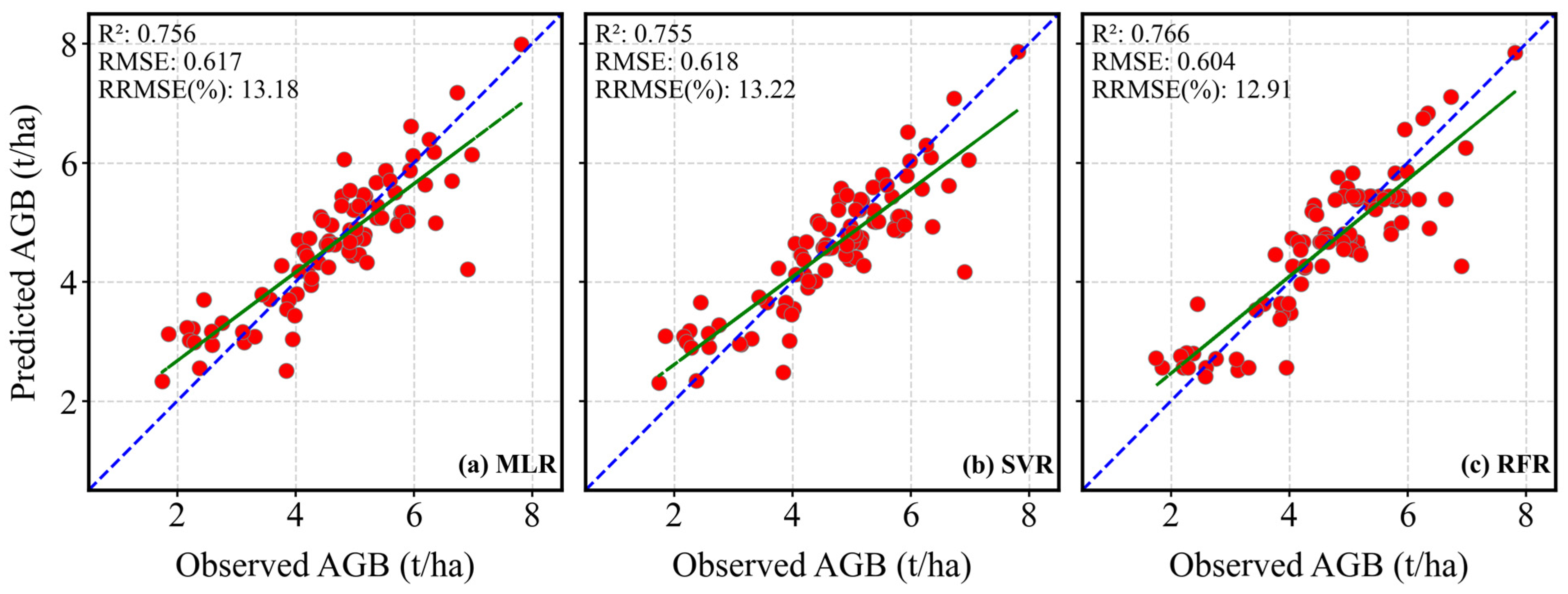
3.5. The Results of Aboveground Biomass and Carbon Stock Using Machine Learning Models

Different machine learning models produced varying results for AGB and carbon estimates. The resulting AGB ranged from 2.30 to 7.99 t/ha (mean: 5.16 t/ha), while AGC ranged from 1.08 to 3.76 t/ha (mean: 2.43 t/ha). The resulting BGB ranged from 0.60 to 2.08 t/ha (mean: 1.34 t/ha), while BGC ranged from 0.16 to 0.54 t/ha (mean: 0.35 t/ha). Total biomass ranged from 2.90 to 10.07 t/ha (mean: 6.49 t/ha), while total carbon ranged from 1.24 to 4.30 t/ha (mean: 2.77 t/ha).

Since multiple tree species were planted during the BTAP program, the distribution of living tree biomass varies for different sites. Non-plantation areas were masked in the biomass map, which showed lower biomass in the north and northeast due to fewer plantations and higher elevations. Biomass depends on tree age, with mature trees having higher biomass, and denser vegetation yielding higher biomass [71]. AGB values ranged from 1.15–12.38 t/ha, with 78% of plantation sites having high biomass (4–8 t/ha) and 22% having low biomass (1–4 t/ha). Across the study area, 60.67% had AGB values of 1–6 t/ha, while 39.33% ranged from 6–8 t/ha. Southern and central regions showed a high amount of biomass since more plantation activities occurred in these regions. On the other hand, the north regions showed lower biomass. The predicted AGB using the random forest model ranged from 2.42–7.90 t/ha.

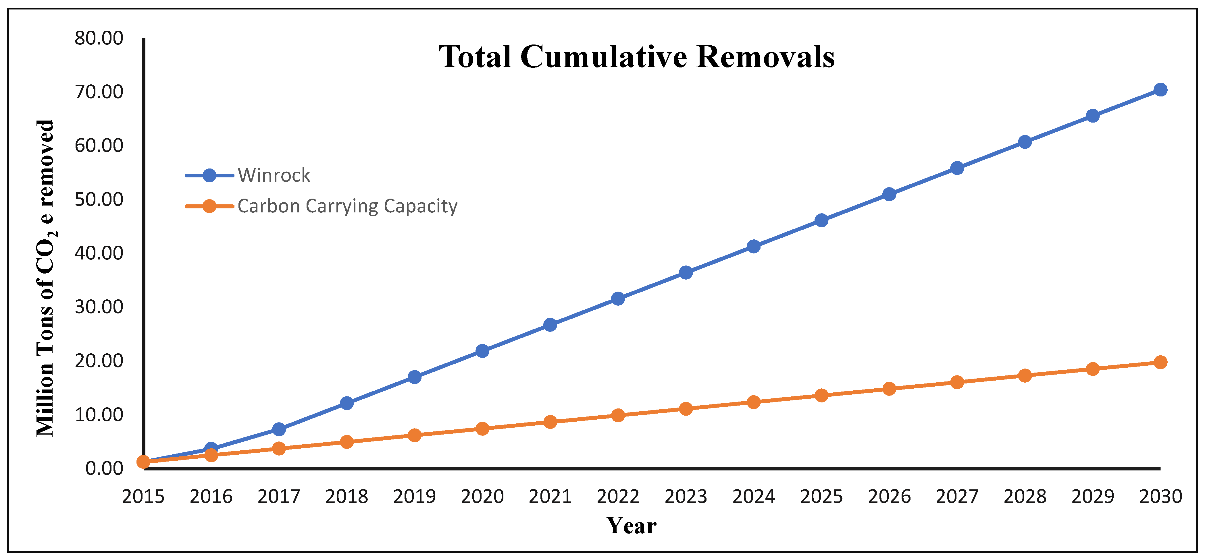
3.6. The Results of Carbon Sequestration Potential in the Study Area

The BTAP implementation in KP Province and forest recovery are expected to enhance carbon sequestration potential over time, provided proper management practices are adopted, and human disturbances are minimized. CSP was calculated using the following equation:

CSP = (102 ± 15) × − (2.82) = 99.18 ± 15 t/ha
(Divide this value by forest age)
CSP = 99.18 ± 15 t/ha ÷ 15 years = 6.61 t/ha/yr
(When forest age is assumed to be 15 years at maturity)

This is a generic value of carbon carrying capacity (CCC) for the plantation forests having Eucalyptus and Robinia as major species [72,73]. The carbon sequestration potential (CSP) for plantation forests dominated by Eucalyptus and Robinia is estimated at 99.18 ± 15 t/ha. Assuming a 15-year rotation age, the annual carbon sequestration potential is 6.61 t/ha/yr under ideal conditions, including suitable temperature, precipitation, site quality, soil type, reduced human disturbance, and proper management. According to carbon carrying capacity the plantation site can store 19.74 million tons of carbon up to 2030 (Figure 12).

Carbon stock refers to the total carbon that is present at the time of inventory. Carbon sequestration is the process of carbon removal from the atmosphere and storing it in reservoirs [74]. Effective CO₂ mitigation requires measuring carbon sequestration potential across all reservoirs, including forests. Young forests act as significant carbon sinks, whereas older forests store carbon at a slower rate. Achieving CCC and reducing human activities in forests are critical for lowering carbon emissions.

Winrock International has developed tools to estimate the carbon sequestration potential of Forest Landscape Restoration (FLR) activities using generalized data on growth rates and carbon accumulation. However, these tools often overlook site-specific factors like plantation failure rates, species selection, site conditions, management practices, and unforeseen events like pest infestation or extreme weather which affect accuracy. Incorporating local data on survival rates and specific species growth performance in that particular region is crucial for reliable estimates. Using Winrock’s database, it was projected that plantation sites could sequester approximately 70.4 million tons of carbon by 2030, based on inputs like plantation year and species per hectare (Figure 12). However, these estimates are likely inflated as they do not account for site-specific challenges (failure rate). Approximately 90% of plantation sites in the study area consist of broadleaved species.

4. Discussion

4.1. Stand Structure

The plantation sites mainly consisted of broadleaved species with Chir pine (Pinus roxburghii) being the only conifer. Eucalyptus was the most planted species, followed by Robinia pseudoacacia, alongside others like Ailanthus altissima, Melia azedarach, Acacia modesta, and Olea ferruginea. The plantation elevations ranged from 109 m to 3013 m, with a mean of 719 m. Trees were spaced 10 by 10 feet, resulting in 1076 trees per hectare. Most plantations are young with faster growth rates, offering high potential for carbon sequestration and trading. However, 90% of the study area at each site is monoculture, which is less resilient compared to mixed-species plantations that are more robust against pests, diseases, and climate extremes [75]. Studies [76,77] highlight the dominance of Eucalyptus in KP’s BTAP plantations, primarily due to community preference for this species on their land. However, researchers recommend prioritizing mixed species plantations to address climate challenges and biodiversity loss effectively [78,79]. Diverse forests are more resilient and adaptable to climate change [80] and support better biodiversity than monocultures [81]. The plantation of mixed species plantations are typically more productive, economically beneficial, and healthier [78]. They also enhance soil carbon stock and drought resilience in arid regions [82]. Monocultures, on the other hand, can displace native biodiversity, promote invasive species [83], reduce aboveground carbon stock [84], and decrease in soil organic carbon [85].

4.2. Major Drivers for Forest AGB Dynamics

The provincial government launched BTAP afforestation project in 2014, resulting in increasing biomass in KP. Fast growing species like Eucalyptus camaldulensis and Robinia pseudoacacia were planted for land reclamation and to reduce reliance on natural forests by providing fuelwood and other resources, boosting AGB storage in the study area. According to yield tables for even-aged plantations, stand productivity declines significantly in mature forests [86]. Young forests exhibit rapid growth and absorb CO₂ more efficiently than most ecosystems, with forest biomass accounting for about 90% of all terrestrial living biomass [87]. However, as forests age, the proportion of aboveground biomass decreases. In this study, carbon stock values ranged from 0.68 t/ha to 7.33 t/ha.

The BTAP afforestation initiative has significantly increased forest cover, enhancing the terrestrial ecosystem’s carbon sequestration potential while reducing local dependence on natural forests for fuelwood and timber. The current data are crucial for calculating carbon credits from BTAP, which totaled 2.06 million credits by 2020. Carbon credit contributes significantly to the country’s greenhouse gas (GHG) reduction efforts. Furthermore, the potential revenue from carbon credits can be estimated based on their market price. The findings indicate that KP BTAP plantations have significant potential to mitigate climate change. Protecting these plantations from felling can further reduce carbon emissions and enhance atmospheric carbon sequestration.

4.3. Role of Remote Sensing in Estimating AGB

For estimating AGB, remote sensing data plays a crucial role due to its extensive spatial coverage, better revisit time, availability of multimodal data (optical, SAR, and LiDAR), cost-effectiveness, and integration with advance methods. Recent advancements in remote sensing have significantly enhanced the estimation of AGB during afforestation activities. Remote sensing has a critical role in providing accurate and efficient estimations of forest AGB, which is essential for sustainable forest management, understanding the global carbon cycle. Selecting appropriate remote sensing variables is essential for accurate AGB estimation [88]. Vegetation indices such as NDVI, SAVI, and RENDVI, along with Sentinel-1 VV and VH polarization data, were used. While vegetation indices minimize background effects, more ground data is needed for multi-source sensors. VH polarization is sensitive to biomass and volume scattering, whereas VV polarization detects moisture beneath the canopy [89]. Combining optical and SAR data enhances AGB estimation accuracy.

4.4. Importance of Data Fusion and Machine Learning for AGB

Optical data demonstrated efficient performance for AGB estimation; however, the optical data for regions with dense vegetation and high biomass face saturation issues [90]. Additionally, optical data have poor penetrability which limits their capabilities to capture the forest’s horizontal structure, missing key components like stem and branch biomass [91]. SAR signals, especially long-wave bands like L-band and P-band, can penetrate the canopy and record vertical structure. However, SAR signals are prone to saturation in high biomass or dense canopies and are sensitive to terrain, reducing accuracy [92,93]. Optical/SAR data fusion can provide a useful and efficient alternative for estimating AGB.

Recent studies have demonstrated the effectiveness of fusing multimodal data for improving AGB estimation accuracy. In Guangdong Province, China, Shen et al., 2018 combined optical and SAR images to map subtropical forest AGB, showing strong correlations [94]. Similarly, Cutler et al., 2012 used Landsat TM and JERS-1 L-band SAR to quantify the AGB in tropical forest at three distinct sites, achieving improved accuracy [95]. While Sentinel-1A has limited penetration capacity, combining Sentinel-1 and Sentinel-2 data has proven more effective than using single datasets. These free, globally available remote sensing systems enable reliable, long-term forest AGB monitoring.

Machine learning techniques combined with remote sensing are effective for precisely monitoring forest resources over large spatial scales. However, challenges remain, such as estimation errors due to temporal mismatches between the field observation and remote sensing imagery. This particularly occurs due to non-availability of cloud-free data during the times when field data were collected. Research suggests that data from multiple remote sensing sources can be used to efficiently derived AGB and AGC for forests [96]. Previous studies that estimated biomass primarily relied on classical statistical techniques like linear regression, which are linear in nature [97]. However, the linear methods are sometimes not adequate to capture the nonlinear interactions between forest AGB and remote sensing data. The use of machine learning models such as RFR addresses this limitation by modelling nonlinear relationships and integrating data from multiple sources to improve prediction accuracy [98,99].

4.5. Implications of This Study

This study directly addresses the global climate change challenge by quantifying carbon sequestration. It emphasizes the role of afforestation in mitigating climate change impacts, specifically in a developing country such as Pakistan, which is vulnerable to climate-related risks. By providing accurate estimates of AGB, and carbon sequestration potential, this research supports national carbon accounting and reporting obligations under the Kyoto Protocol. This is crucial for international commitments like the Bonn Challenge. Additionally, utilizing multimodal data and machine learning models improves the accuracy and scalability of biomass and carbon stock estimation. These methodological improvements demonstrate the potential of remote sensing and machine learning in forest management. The finding provides a scientific foundation for policymaking, particularly in guiding afforestation projects like BTAP. Additionally, it aligns with sustainable development goals (SDGs). This evidence can justify investments in afforestation programs and inspire similar initiatives globally. The estimation of carbon credits from the BTAP plantation underscores the economic potential of afforestation projects in international carbon markets. This can be a significant incentive for developing countries to expand their green initiatives. Focused on Pakistan’s KP region the study methodology and findings have implications for other regions with similar environmental conditions. It sets a precedent for leveraging technology to monitor and evaluate large-scale afforestation projects globally. In short, this study bridges science and policy by providing actionable insights into climate change mitigation, natural resource management, and sustainable development.

Kumar et al., 2021 [100] estimated aboveground and belowground carbon stock at 59.62 t/ha and 18.61 t/ha, respectively, while Mishra [101] reported 55.44 t/ha, 12.54 t/ha, and 67.98 t/ha for aboveground, belowground, and total carbon stock. These higher carbon stocks are attributed to older trees with mean DBH of 17.4 ± 1.5 cm and height of 9.6 ± 1.8 m, compared to the current study mean DBH of 4.54 cm and height of 3.9 m. Tree age, diameter, site quality, soil type, and stand density significantly influence biomass [102,103]. Labata et al., 2012 [104] highlighted the high carbon storage potential of Eucalyptus plantations due to high-density planting, favorable growth patterns, and suitable soil conditions.

Reforestation programs have increased carbon stock, as evident from the results. According to Ali et al., [18] the carbon stock in KP province was 144.71 million tons (127.66 t/ha on average) and rose to 145.27 million tons by 2020 due to BTAP plantations. Additionally, 0.287 million hectares, including plantations and enclosures, were restored during the six years of the BTAP project [68]. However, carbon stock in the BTAP enclosure site was not assessed in this study.

This study assumed no harvesting of BTAP planted trees in KP Province for carbon sequestration estimates. Future studies should account for potential harvesting scenarios to evaluate the program’s long term carbon sequestration potential.

4.6. Limitations of Current Study and Future Work

In this study, the AGB of forest sites was successfully estimated; however, certain limitations remain that can be addressed in future research. A total of 310 sampling plots were used across the BTAP plantation, which produced decent results with machine learning models. However, given the large-scale nature of BTAP, expanding field data coverage in future studies could enhance the representativeness of samples and improve the overall accuracy of AGB estimations in the study area. This study utilized Sentinel-1 and Sentinel-2 data for AGB estimation. Future research could incorporate data from additional sensors to provide complementary spectral and structural information, further improving the accuracy of estimations. The field of machine learning is advancing rapidly, with increasingly sophisticated methods being developed. While the models used in this study performed well, future studies could explore the application of advanced deep learning models to further improve AGB estimation in forest ecosystems. Finally, the importance of high-resolution satellite and UAV data cannot be overstated. High spatial, spectral, and temporal resolution data can significantly enhance biomass estimation, supporting global sustainability initiatives such as the Sustainable Development Goals (SDGs) and REDD+ objectives.

5. Conclusions

This study’s main contribution lies in the application of a fusion approach combining Sentinel-1 and Sentinel-2 data with machine learning models to estimate AGB and CSP in forest restoration areas. The key findings were as follows:

• Using machine learning models such as MLR, SVR, and RFR, AGB estimation was successfully conducted, with RFR demonstrating superior performance (R² = 0.766) compared to the other models.
• The total estimated biomass ranged from 1.104 to 1.278 million tons, with an average of 5.55 t/ha to 6.42 t/ha. Correspondingly, carbon stock ranged from 0.519 to 0.6 million tons, with an average of 2.61 t/ha to 3.02 t/ha, sequestering 2.06 million tons of CO₂ equivalent by 2020, with a mean of 10.33 t/ha. Additionally, the CSP for the study area was estimated at 99.18 ± 15 t/ha.
• The integration of multimodal remote sensing data with machine learning models can not only produce reliable results for biomass mapping but also reduce labor intensity and improve accuracy under varied environmental conditions. Furthermore, the ability of SAR data to operate in all-weather conditions minimized the impact of clouds, shadows, and rain, enhancing the robustness of the method.

This study underscores the importance of protecting existing plantations, increasing the plantation of indigenous species, and integrating remote sensing technologies for sustainable forest management and carbon sequestration. The results demonstrate that a fusion mechanism of optical and SAR data is a valuable, efficient, and cost-effective approach for creating reliable spatial mapping of AGB, offering a critical tool for forest management, carbon sequestration assessment, and forest protection efforts. Nonetheless, there is a need to use these methods across different forest types and environmental conditions to further validate their applicability and scalability.

References

1. Raihan, A.; Begum, R.; Said, M.; Abdullah, S.M.S. Climate change mitigation options in the forestry sector of Malaysia. J. Kejuruter. 2018, 1, 89–98. [Google Scholar] [CrossRef]
2. Volkova, L.; Roxburgh, S.H.; Weston, C.J.; Benyon, R.G.; Sullivan, A.L.; Polglase, P.J. Importance of disturbance history on net primary productivity in the world’s most productive forests and implications for the global carbon cycle. Glob. Change Biol. 2018, 24, 4293–4303. [Google Scholar] [CrossRef] [PubMed]
3. Miura, S.; Amacher, M.; Hofer, T.; San-Miguel-Ayanz, J.; Thackway, R. Protective functions and ecosystem services of global forests in the past quarter-century. For. Ecol. Manag. 2015, 352, 35–46. [Google Scholar] [CrossRef]
4. Lorenz, K. Carbon Sequestration in Forest Ecosystems; Springer: Berlin/Heidelberg, Germany, 2010. [Google Scholar]
5. Thomas, S.C.; Martin, A.R. Carbon content of tree tissues: A synthesis. Forests 2012, 3, 332–352. [Google Scholar] [CrossRef]
6. Chave, J.; Réjou-Méchain, M.; Búrquez, A.; Chidumayo, E.; Colgan, M.S.; Delitti, W.B.; Duque, A.; Eid, T.; Fearnside, P.M.; Goodman, R.C. Improved allometric models to estimate the aboveground biomass of tropical trees. Glob. Change Biol. 2014, 20, 3177–3190. [Google Scholar] [CrossRef]
7. Houghton, R.; Hall, F.; Goetz, S.J. Importance of biomass in the global carbon cycle. J. Geophys. Res. Biogeosci. 2009, 114, G00E03. [Google Scholar] [CrossRef]
8. Santini, N.S.; Adame, M.F.; Nolan, R.H.; Miquelajauregui, Y.; Piñero, D.; Mastretta-Yanes, A.; Cuervo-Robayo, Á.P.; Eamus, D. Storage of organic carbon in the soils of Mexican temperate forests. For. Ecol. Manag. 2019, 446, 115–125. [Google Scholar] [CrossRef]
9. Pan, Y.; Birdsey, R.A.; Fang, J.; Houghton, R.; Kauppi, P.E.; Kurz, W.A.; Phillips, O.L.; Shvidenko, A.; Lewis, S.L.; Canadell, J.G. A large and persistent carbon sink in the world’s forests. Science 2011, 333, 988–993. [Google Scholar] [CrossRef]
10. FAO. Global Forest Resources Assessment; FAO: Rome, Italy, 2010. [Google Scholar]
11. Streck, C.; Scholz, S.M. The role of forests in global climate change: Whence we come and where we go. Int. Aff. 2006, 82, 861–879. [Google Scholar] [CrossRef]
12. Li, W.; Chen, E.; Li, Z.; Ke, Y.; Zhan, W. Forest aboveground biomass estimation using polarization coherence tomography and PolSAR segmentation. Int. J. Remote Sens. 2015, 36, 530–550. [Google Scholar] [CrossRef]
13. Chen, L.-C.; Guan, X.; Li, H.-M.; Wang, Q.-K.; Zhang, W.-D.; Yang, Q.-P.; Wang, S.-L. Spatiotemporal patterns of carbon storage in forest ecosystems in Hunan Province, China. For. Ecol. Manag. 2019, 432, 656–666. [Google Scholar] [CrossRef]
14. Shaharuddin, M.I. Forest management systems in Southeast Asia. In Managing the Future of Southeast Asia’s Valuable Tropical Rainforests: A Practitioner’s Guide to Forest Genetics; Springer: Berlin/Heidelberg, Germany, 2011; pp. 1–20. [Google Scholar]
15. Liu, T.Y.; Mao, F.J.; Li, X.J.; Xing, L.Q.; Dong, L.F.; Zheng, J.L.; Zhang, M.; HQ, D. Spatiotemporal dynamic simulation on aboveground carbon storage of bamboo forest and its influence factors in Zhejiang Province, China. Ying Yong Sheng Tai Xue Bao = J. Appl. Ecol. 2019, 30, 1743–1753. [Google Scholar]
16. Nizami, S.M. The inventory of the carbon stocks in sub tropical forests of Pakistan for reporting under Kyoto Protocol. J. For. Res. 2012, 23, 377–384. [Google Scholar] [CrossRef]
17. Nizami, S.M. Estimation of Carbon Stocks in Subtropical Managed and Unmanaged Forests of Pakistan. Ph.D. Thesis, Department of Forestry and Range Management, Faculty of Forestry, Range Management and Wildlife, Pir Mehr Ali Shah Arid Agricultural University, Rawalpindi, Pakistan, 2010. [Google Scholar]
18. Ali, A.; Ashraf, M.I.; Gulzar, S.; Akmal, M. Estimation of forest carbon stocks in temperate and subtropical mountain systems of Pakistan: Implications for REDD+ and climate change mitigation. Environ. Monit. Assess. 2020, 192, 198. [Google Scholar] [CrossRef] [PubMed]
19. Ali, A. Forest Reference Emission Level of Khyber Pakhtunkhwa; Pakistan Forest Institute: Peshawar, Pakistan, 2017.
20. Schneider, L.; La Hoz Theuer, S. Environmental integrity of international carbon market mechanisms under the Paris Agreement. Clim. Policy 2019, 19, 386–400. [Google Scholar] [CrossRef]
21. Khan, K.; Khokar, M.F.; Khan, S.N.; Khan, J.A. Characterizing Forest Cover Dynamics in the Khyber Pakhtunkhwa Region Using Remote Sensing. In Proceedings of the 2024 International Conference on Frontiers of Information Technology (FIT), Islamabad, Pakistan, 9–10 December 2024; pp. 1–6. [Google Scholar]
22. Khan, K.; Iqbal, J.; Ali, A.; Khan, S. Assessment of Sentinel-2-derived vegetation indices for the estimation of above-ground biomass/carbon stock, temporal deforestation and carbon emissions estimation in the moist temperate forests of Pakistan. Appl. Ecol. Environ. Res. 2020, 18, 783–815. [Google Scholar] [CrossRef]
23. Khan, I.A.; Ali, A.; Hussain, M.; Ullah, H.; Urrehman, A.; Ali, N.; Khattak, M. Tree biomass and carbon estimation of Pinus roxburghii and Eucalyptus camaldulensis. J. Biodivers. Environ. Sci. 2018, 13, 8–16. [Google Scholar]
24. Avtar, R.; Suzuki, R.; Sawada, H. Natural forest biomass estimation based on plantation information using PALSAR data. PLoS ONE 2014, 9, e86121. [Google Scholar] [CrossRef]
25. Zhang, Y.; Yao, Y.; Wang, X.; Liu, Y.; Piao, S. Mapping spatial distribution of forest age in China. Earth Space Sci. 2017, 4, 108–116. [Google Scholar] [CrossRef]
26. Ali, A.; Xu, M.-S.; Zhao, Y.-T.; Zhang, Q.-Q.; Zhou, L.-L.; Yang, X.-D.; Yan, E.-R. Allometric biomass equations for shrub and small tree species in subtropical China. Silva Fenn. 2015, 49, 1275. [Google Scholar] [CrossRef]
27. Kumar, L.; Mutanga, O. Remote sensing of above-ground biomass. Remote Sens. 2017, 9, 935. [Google Scholar] [CrossRef]
28. Lu, D. The potential and challenge of remote sensing-based biomass estimation. Int. J. Remote Sens. 2006, 27, 1297–1328. [Google Scholar] [CrossRef]
29. West, P.W.; West, P.W. Tree and Forest Measurement; Springer: Berlin/Heidelberg, Germany, 2009; Volume 20. [Google Scholar]
30. Cao, L.; Coops, N.C.; Innes, J.L.; Sheppard, S.R.; Fu, L.; Ruan, H.; She, G. Estimation of forest biomass dynamics in subtropical forests using multi-temporal airborne LiDAR data. Remote Sens. Environ. 2016, 178, 158–171. [Google Scholar] [CrossRef]
31. Shen, W.; Li, M.; Huang, C.; Wei, A. Quantifying live aboveground biomass and forest disturbance of mountainous natural and plantation forests in Northern Guangdong, China, based on multi-temporal Landsat, PALSAR and field plot data. Remote Sens. 2016, 8, 595. [Google Scholar] [CrossRef]
32. Yin, H.; Khamzina, A.; Pflugmacher, D.; Martius, C. Forest cover mapping in post-Soviet Central Asia using multi-resolution remote sensing imagery. Sci. Rep. 2017, 7, 1375. [Google Scholar] [CrossRef]
33. Valjarević, A.; Djekić, T.; Stevanović, V.; Ivanović, R.; Jandziković, B. GIS numerical and remote sensing analyses of forest changes in the Toplica region for the period of 1953–2013. Appl. Geogr. 2018, 92, 131–139. [Google Scholar] [CrossRef]
34. Chen, Y.; Li, L.; Lu, D.; Li, D. Exploring bamboo forest aboveground biomass estimation using Sentinel-2 data. Remote Sens. 2018, 11, 7. [Google Scholar] [CrossRef]
35. Haywood, A.; Stone, C.; Jones, S. The potential of sentinel satellites for large area aboveground forest biomass mapping. In Proceedings of the IGARSS 2018—2018 IEEE International Geoscience and Remote Sensing Symposium, Valencia, Spain, 22–27 July 2018; pp. 9030–9033. [Google Scholar]
36. Kellndorfer, J.; Walker, W.; LaPoint, E.; Kirsch, K.; Bishop, J.; Fiske, G. Statistical fusion of Lidar, InSAR, and optical remote sensing data for forest stand height characterization: A regional-scale method based on LVIS, SRTM, Landsat ETM+, and ancillary data sets. J. Geophys. Res. Biogeosci. 2010, 115, G00E08. [Google Scholar] [CrossRef]
37. Chang, J.; Shoshany, M. Mediterranean shrublands biomass estimation using Sentinel-1 and Sentinel-2. In Proceedings of the 2016 IEEE International Geoscience and Remote Sensing Symposium (IGARSS), Beijing, China, 10–15 July 2016; pp. 5300–5303. [Google Scholar]
38. Li, S. Forest Aboveground Biomass Estimation Using Multi-Source Remote Sensing Data in Temperate Forests. Ph.D. Thesis, State University of New York College of Environmental Science and Forestry, Syracuse, NY, USA, 2019. [Google Scholar]
39. Ma, J.; Zhang, W.; Ji, Y.; Huang, J.; Huang, G.; Wang, L. Total and component forest aboveground biomass inversion via LiDAR-derived features and machine learning algorithms. Front. Plant Sci. 2023, 14, 1258521. [Google Scholar] [CrossRef]
40. Khan, S.N.; Li, D.; Maimaitijiang, M. A geographically weighted random forest approach to predict corn yield in the US corn belt. Remote Sens. 2022, 14, 2843. [Google Scholar] [CrossRef]
41. Wang, P.; Tan, S.; Zhang, G.; Wang, S.; Wu, X. Remote sensing estimation of forest aboveground biomass based on Lasso-SVR. Forests 2022, 13, 1597. [Google Scholar] [CrossRef]
42. Nguyen, A.; Saha, S. Machine Learning and Multi-source Remote Sensing in Forest Carbon Stock Estimation: A Review. arXiv 2024, arXiv:2411.17624. [Google Scholar]
43. Molto, Q.; Rossi, V.; Blanc, L. Error propagation in biomass estimation in tropical forests. Methods Ecol. Evol. 2013, 4, 175–183. [Google Scholar] [CrossRef]
44. Malenovský, Z.; Rott, H.; Cihlar, J.; Schaepman, M.E.; García-Santos, G.; Fernandes, R.; Berger, M. Sentinels for science: Potential of Sentinel-1,-2, and-3 missions for scientific observations of ocean, cryosphere, and land. Remote Sens. Environ. 2012, 120, 91–101. [Google Scholar] [CrossRef]
45. Torres, R.; Snoeij, P.; Geudtner, D.; Bibby, D.; Davidson, M.; Attema, E.; Potin, P.; Rommen, B.; Floury, N.; Brown, M. GMES Sentinel-1 mission. Remote Sens. Environ. 2012, 120, 9–24. [Google Scholar] [CrossRef]
46. Lee, J.-S.; Wen, J.-H.; Ainsworth, T.L.; Chen, K.-S.; Chen, A.J. Improved sigma filter for speckle filtering of SAR imagery. IEEE Trans. Geosci. Remote Sens. 2008, 47, 202–213. [Google Scholar]
47. ASF. Alaska Satellite Facility Alos-Palsar Digital Elevation Model (DEM); ASF: Fairbanks, AK, USA, 2012.
48. Baillarin, S.; Meygret, A.; Dechoz, C.; Petrucci, B.; Lacherade, S.; Trémas, T.; Isola, C.; Martimort, P.; Spoto, F. Sentinel-2 level 1 products and image processing performances. In Proceedings of the 2012 IEEE International Geoscience and Remote Sensing Symposium, Munich, Germany, 22–27 July 2012; pp. 7003–7006. [Google Scholar]
49. Rouse, J.W.; Haas, R.H.; Schell, J.A.; Deering, D.W. Monitoring vegetation systems in the great plains with ERTS. In Proceedings of the Third ERTS-1 Symposium NASA, NASA SP-351, Washington, DC, USA, 10–14 December 1974; Volume 351, p. 309. [Google Scholar]
50. Huete, A.R. A soil vegetation adjusted index (SAVI). Remote Sens. Environ. 1988, 25, 295–309. [Google Scholar] [CrossRef]
51. Chen, J.-C.; Yang, C.-M.; Wu, S.-T.; Chung, Y.-L.; Charles, A.L.; Chen, C.-T. Leaf chlorophyll content and surface spectral reflectance of tree species along a terrain gradient in Taiwan’s Kenting National Park. Bot. Stud. 2007, 48, 71–77. [Google Scholar]
52. Shi, L.; Liu, S. Methods of estimating forest biomass: A review. Biomass Vol. Estim. Valorization Energy 2017, 10, 65733. [Google Scholar]
53. Gao, X.; Jiang, Z.; Guo, Q.; Zhang, Y.; Yin, H.; He, F.; Qi, L.; Shi, L. Allometry and Biomass Production of Phyllostachys Edulis Across the Whole Lifespan. Pol. J. Environ. Stud. 2015, 24, 511. [Google Scholar]
54. Ali, A.; Forest Mensuration Officer. Biomass and Carbon Tables for Major Tree Species of Gilgit Baltistan, Pakistan; Gilgit-Baltistan Forests, Wildlife and Environment Department: Gilgit, Pakistan, 2015.
55. Chave, J.; Condit, R.; Lao, S.; Caspersen, J.P.; Foster, R.B.; Hubbell, S.P. Spatial and temporal variation of biomass in a tropical forest: Results from a large census plot in Panama. J. Ecol. 2003, 91, 240–252. [Google Scholar] [CrossRef]
56. Ali, A.; Ashraf, M.I.; Gulzar, S.; Akmal, M. Development of an allometric model for biomass estimation of Pinus roxburghii, growing in subtropical pine forests of Khyber Pakhtunkhwa, Pakistan. Sarhad J. Agric. 2020, 36, 236–244. [Google Scholar] [CrossRef]
57. Ali, A.; Iftikhar, M.; Ahmad, S.; Muhammad, S.; Khan, A. Development of allometric equation for biomass estimation of Cedrus deodara in dry temperate forests of Northern Pakistan. J. Biodivers. Environ. Sci. 2016, 9, 43–50. [Google Scholar]
58. IPCC. Climate Change 2007: Impacts, Adaptation and Vulnerability; IPCC: Geneva, Switzerland, 2001. [Google Scholar]
59. Ali, A.; Ullah, S.; Bushra, S.; Ahmad, N.; Ali, A.; Khan, M.A. Quantifying forest carbon stocks by integrating satellite images and forest inventory data. Austrian J. For. Sci./Cent. Gesamte Forstwes. 2018, 135, 93. [Google Scholar]
60. Pearson, T.R. Measurement Guidelines for the Sequestration of Forest Carbon; US Department of Agriculture, Forest Service, Northern Research Station: Washington, DC, USA, 2007; Volume 18.
61. Smola, A.J.; Schölkopf, B. A tutorial on support vector regression. Stat. Comput. 2004, 14, 199–222. [Google Scholar] [CrossRef]
62. Awad, M.; Khanna, R.; Awad, M.; Khanna, R. Support vector regression. In Efficient Learning Machines: Theories, Concepts, and Applications for Engineers and System Designers; Springer Nature: Berlin/Heidelberg, Germany, 2015; pp. 67–80. [Google Scholar]
63. Hastie, T.; Tibshirani, R.; Friedman, J.H.; Friedman, J.H. The Elements of Statistical Learning: Data Mining, Inference, and Prediction; Springer: Berlin/Heidelberg, Germany, 2009; Volume 2. [Google Scholar]
64. Zhou, G.; Wang, Y.; Jiang, Y.; Yang, Z. Estimating biomass and net primary production from forest inventory data: A case study of China’s Larix forests. For. Ecol. Manag. 2002, 169, 149–157. [Google Scholar] [CrossRef]
65. Cramer, W.; Bondeau, A.; Woodward, F.I.; Prentice, I.C.; Betts, R.A.; Brovkin, V.; Cox, P.M.; Fisher, V.; Foley, J.A.; Friend, A.D. Global response of terrestrial ecosystem structure and function to CO2 and climate change: Results from six dynamic global vegetation models. Glob. Change Biol. 2001, 7, 357–373. [Google Scholar] [CrossRef]
66. Liu, Y.; Wang, Q.; Yu, G.; Zhu, X.; Zhan, X.; Guo, Q.; Yang, H.; Li, S.; Hu, Z. Ecosystems carbon storage and carbon sequestration potential of two main tree species for the Grain for Green Project on China’s hilly Loess Plateau. Shengtai Xuebao/Acta Ecol. Sin. 2011, 31, 4277–4286. [Google Scholar]
67. Bernal, B.; Murray, L.T.; Pearson, T.R. Global carbon dioxide removal rates from forest landscape restoration activities. Carbon Balance Manag. 2018, 13, 22. [Google Scholar] [CrossRef]
68. Khan, K.; Khan, J.A.; Khokhar, M.F.; Khan, S.N.; Iqbal, J. Estimating afforestation related forest cover change using data fusion and machine learning. Environ. Res. Commun. 2024, 6, 115004. [Google Scholar] [CrossRef]
69. Wang, Z.; Du, X. Monitoring Natural World Heritage Sites: Optimization of the monitoring system in Bogda with GIS-based multi-criteria decision analysis. Environ. Monit. Assess. 2016, 188, 384. [Google Scholar] [CrossRef]
70. Gitelson, A.A.; Kaufman, Y.J.; Merzlyak, M.N. Use of a green channel in remote sensing of global vegetation from EOS-MODIS. Remote Sens. Environ. 1996, 58, 289–298. [Google Scholar] [CrossRef]
71. Du, L.; Zhou, T.; Zou, Z.; Zhao, X.; Huang, K.; Wu, H. Mapping forest biomass using remote sensing and national forest inventory in China. Forests 2014, 5, 1267–1283. [Google Scholar] [CrossRef]
72. Siraj, K.; Teshome, B. Potential difference of tree species on carbon sequestration performance and role of forest based industry to the environment (Case of Arsi Forest Enterprise Gambo District). Environ. Pollut. Clim. Change 2017, 1, 2–10. [Google Scholar] [CrossRef]
73. Xanthopoulos, G.; Radoglou, K.; Derrien, D.; Spyroglou, G.; Angeli, N.; Tsioni, G.; Fotelli, M.N. Carbon sequestration and soil nitrogen enrichment in Robinia pseudoacacia L. post-mining restoration plantations. Front. For. Glob. Change 2023, 6, 1190026. [Google Scholar] [CrossRef]
74. Takimoto, A.; Nair, V.D.; Nair, P. Contribution of trees to soil carbon sequestration under agroforestry systems in the West African Sahel. In Advances in Agroforestry; Springer: Berlin/Heidelberg, Germany, 2008; pp. 11–25. [Google Scholar]
75. Hutchison, C.; Gravel, D.; Guichard, F.; Potvin, C. Effect of diversity on growth, mortality, and loss of resilience to extreme climate events in a tropical planted forest experiment. Sci. Rep. 2018, 8, 15443. [Google Scholar] [CrossRef]
76. Ullah, I.; Saleem, A.; Ansari, L.; Ali, N.; Ahmad, N.; Dar, N.; Din, N. Growth and survival of multipurpose species; Assessing Billion Tree Afforestation Project (BTAP), the Bonn Challenge initiative. Appl. Ecol. Environ. Res. 2020, 18, 2057–2072. [Google Scholar] [CrossRef]
77. Nazir, N.; Farooq, A.; Ahmad Jan, S.; Ahmad, A. A system dynamics model for billion trees tsunami afforestation project of Khyber Pakhtunkhwa in Pakistan: Model application to afforestation activities. J. Mt. Sci. 2019, 16, 2640–2653. [Google Scholar] [CrossRef]
78. Liu, C.L.C.; Kuchma, O.; Krutovsky, K.V. Mixed-species versus monocultures in plantation forestry: Development, benefits, ecosystem services and perspectives for the future. Glob. Ecol. Conserv. 2018, 15, e00419. [Google Scholar] [CrossRef]
79. Brockerhoff, E.G.; Barbaro, L.; Castagneyrol, B.; Forrester, D.I.; Gardiner, B.; González-Olabarria, J.R.; Lyver, P.O.B.; Meurisse, N.; Oxbrough, A.; Taki, H. Forest biodiversity, ecosystem functioning and the provision of ecosystem services. Biodivers. Conserv. 2017, 26, 3005–3035. [Google Scholar] [CrossRef]
80. Pretzsch, H.; Forrester, D.I.; Bauhus, J. Mixed-Species Forests. Ecology and Management; Springer Nature: Chan, Switzerland, 2017; Volume 653. [Google Scholar]
81. Wang, X.; Hua, F.; Wang, L.; Wilcove, D.S.; Yu, D.W. The biodiversity benefit of native forests and mixed-species plantations over monoculture plantations. Divers. Distrib. 2019, 25, 1721–1735. [Google Scholar] [CrossRef]
82. Gong, C.; Tan, Q.; Xu, M.; Liu, G. Mixed-species plantations can alleviate water stress on the Loess Plateau. For. Ecol. Manag. 2020, 458, 117767. [Google Scholar] [CrossRef]
83. Kull, C.A.; Harimanana, S.L.; Andrianoro, A.R.; Rajoelison, L.G. Divergent perceptions of the ‘neo-Australian’ forests of lowland eastern Madagascar: Invasions, transitions, and livelihoods. J. Environ. Manag. 2019, 229, 48–56. [Google Scholar] [CrossRef]
84. Heilmayr, R.; Echeverría, C.; Lambin, E.F. Impacts of Chilean forest subsidies on forest cover, carbon and biodiversity. Nat. Sustain. 2020, 3, 701–709. [Google Scholar] [CrossRef]
85. Hong, S.; Yin, G.; Piao, S.; Dybzinski, R.; Cong, N.; Li, X.; Wang, K.; Peñuelas, J.; Zeng, H.; Chen, A. Divergent responses of soil organic carbon to afforestation. Nat. Sustain. 2020, 3, 694–700. [Google Scholar] [CrossRef]
86. Ryan, M.G.; Binkley, D.; Fownes, J.H. Age-related decline in forest productivity: Pattern and process. Adv. Ecol. Res. 1997, 27, 213–262. [Google Scholar]
87. Dixon, R.K.; Solomon, A.; Brown, S.; Houghton, R.; Trexier, M.; Wisniewski, J. Carbon pools and flux of global forest ecosystems. Science 1994, 263, 185–190. [Google Scholar] [CrossRef]
88. Lu, D.; Chen, Q.; Wang, G.; Liu, L.; Li, G.; Moran, E. A survey of remote sensing-based aboveground biomass estimation methods in forest ecosystems. Int. J. Digit. Earth 2016, 9, 63–105. [Google Scholar] [CrossRef]
89. Hess, L.L.; Melack, J.M.; Filoso, S.; Wang, Y. Delineation of inundated area and vegetation along the Amazon floodplain with the SIR-C synthetic aperture radar. IEEE Trans. Geosci. Remote Sens. 1995, 33, 896–904. [Google Scholar] [CrossRef]
90. Maimaitijiang, M.; Sagan, V.; Sidike, P.; Daloye, A.M.; Erkbol, H.; Fritschi, F.B. Crop monitoring using satellite/UAV data fusion and machine learning. Remote Sens. 2020, 12, 1357. [Google Scholar] [CrossRef]
91. Myneni, R.B.; Dong, J.; Tucker, C.J.; Kaufmann, R.K.; Kauppi, P.E.; Liski, J.; Zhou, L.; Alexeyev, V.; Hughes, M. A large carbon sink in the woody biomass of Northern forests. Proc. Natl. Acad. Sci. USA 2001, 98, 14784–14789. [Google Scholar] [CrossRef]
92. Le Toan, T.; Beaudoin, A.; Riom, J.; Guyon, D. Relating forest biomass to SAR data. IEEE Trans. Geosci. Remote Sens. 1992, 30, 403–411. [Google Scholar] [CrossRef]
93. Dobson, M.C.; Ulaby, F.T.; LeToan, T.; Beaudoin, A.; Kasischke, E.S.; Christensen, N. Dependence of radar backscatter on coniferous forest biomass. IEEE Trans. Geosci. Remote Sens. 1992, 30, 412–415. [Google Scholar] [CrossRef]
94. Shen, W.; Li, M.; Huang, C.; Tao, X.; Wei, A. Annual forest aboveground biomass changes mapped using ICESat/GLAS measurements, historical inventory data, and time-series optical and radar imagery for Guangdong province, China. Agric. For. Meteorol. 2018, 259, 23–38. [Google Scholar] [CrossRef]
95. Cutler, M.; Boyd, D.S.; Foody, G.M.; Vetrivel, A. Estimating tropical forest biomass with a combination of SAR image texture and Landsat TM data: An assessment of predictions between regions. ISPRS J. Photogramm. Remote Sens. 2012, 70, 66–77. [Google Scholar] [CrossRef]
96. Zhao, P.; Lu, D.; Wang, G.; Liu, L.; Li, D.; Zhu, J.; Yu, S. Forest aboveground biomass estimation in Zhejiang Province using the integration of Landsat TM and ALOS PALSAR data. Int. J. Appl. Earth Obs. Geoinf. 2016, 53, 1–15. [Google Scholar] [CrossRef]
97. Dong, J.; Kaufmann, R.K.; Myneni, R.B.; Tucker, C.J.; Kauppi, P.E.; Liski, J.; Buermann, W.; Alexeyev, V.; Hughes, M.K. Remote sensing estimates of boreal and temperate forest woody biomass: Carbon pools, sources, and sinks. Remote Sens. Environ. 2003, 84, 393–410. [Google Scholar] [CrossRef]
98. Ali, I.; Greifeneder, F.; Stamenkovic, J.; Neumann, M.; Notarnicola, C. Review of machine learning approaches for biomass and soil moisture retrievals from remote sensing data. Remote Sens. 2015, 7, 16398–16421. [Google Scholar] [CrossRef]
99. Baghdadi, N.; Le Maire, G.; Bailly, J.-S.; Osé, K.; Nouvellon, Y.; Zribi, M.; Lemos, C.; Hakamada, R. Evaluation of ALOS/PALSAR L-band data for the estimation of Eucalyptus plantations aboveground biomass in Brazil. IEEE J. Sel. Top. Appl. Earth Obs. Remote Sens. 2014, 8, 3802–3811. [Google Scholar] [CrossRef]
100. Kumar, M.; Kumar, A.; Kumar, R.; Konsam, B.; Pala, N.A.; Bhat, J.A. Carbon stock potential in Pinus roxburghii forests of Indian Himalayan regions. Environ. Dev. Sustain. 2021, 23, 12463–12478. [Google Scholar] [CrossRef]
101. Mishra, B. Assessment of the soil and tree carbon stocks of a Chir pine forest in Garhwal Himalaya India. Int. J. Geol. Earth Environ. Sci. 2017, 7, 19–24. [Google Scholar]
102. Li, C.; Zha, T.; Liu, J.; Jia, X. Carbon and nitrogen distribution across a chronosequence of secondary lacebark pine in China. For. Chron. 2013, 89, 192–198. [Google Scholar] [CrossRef]
103. Amir, M.; Liu, X.; Ahmad, A.; Saeed, S.; Mannan, A.; Muneer, M.A. Patterns of Biomass and Carbon Allocation across Chronosequence of Chir Pine (Pinus roxburghii) Forest in Pakistan: Inventory-Based Estimate. Adv. Meteorol. 2018, 2018, 3095891. [Google Scholar] [CrossRef]
104. Labata, M.M.; Aranico, E.C.; Tabaranza, A.C.E.; Patricio, J.H.P.; Amparad, R.F., Jr. Carbon stock assessment of three selected agroforestry systems in Bukidnon, Philippines. Adv. Environ. Sci. 2012, 4, 5–11. [Google Scholar]
Figure 1. Maps of study area (Khyber Pakhtunkhwa, Pakistan).
Remotesensing 17 00934 g001
Figure 2. Methodology flowchart of the study.
Remotesensing 17 00934 g002
Figure 3. Training and testing data distribution.
Remotesensing 17 00934 g003
Figure 4. Correlation between AGB and vegetation indices. The bottom triangle displays the correlation coefficients, the diagonal shows the distribution of each variable, and the top triangle presents their relationships in a scatterplot.
Remotesensing 17 00934 g004
Figure 5. Derived vegetation indices from Sentinel-2 imagery and VV and VH polarization bands of Sentinel-1.
Remotesensing 17 00934 g005
Figure 6. Scatterplot showing the relationship, regression equation and R-square value between broadband, narrow red-edge band vegetation indices and aboveground biomass estimated through each equation.
Remotesensing 17 00934 g006
Figure 7. Scatterplots of actual vs. predicted biomass using optical and SAR data with (a) MLR, (b) SVR, and (c) RFR.
Remotesensing 17 00934 g007
Figure 8. Scatterplots of actual vs. predicted biomass using optical data with (a) MLR, (b) SVR, and (c) RFR.
Remotesensing 17 00934 g008
Figure 9. Scatterplots of actual vs. predicted biomass using SAR data with (a) MLR, (b) SVR, and (c) RFR.
Remotesensing 17 00934 g009
Figure 10. Training and testing data aboveground biomass (AGB) distribution of actual data and those observed from machine learning models.
Remotesensing 17 00934 g010
Figure 11. Aboveground biomass map of the study area plantation forests predicted using random forest regression.
Remotesensing 17 00934 g011
Figure 12. Carbon sequestration potential of plantation sites using Winrock and carbon carrying capacity.
Remotesensing 17 00934 g012