Plastic Litter Detection in the Environment Using Hyperspectral Aerial Remote Sensing and Machine Learning

Abstract

Plastic waste has become a critical environmental issue, necessitating effective methods for detection and monitoring. This article presents a machine-learning-based methodology and embedded solution to detect plastic waste in the environment using an airborne hyperspectral sensor operating in the short-wave infrared (SWIR) band. Experimental data were obtained from drone flights in several case studies in natural and controlled environments. Data were preprocessed to simply equalize the spectra across the whole band and across different environmental conditions, and machine learning techniques were applied to detect plastics even in real-time. Several algorithms for spectrum calibration, feature selection, and classification were optimized and compared to obtain an optimal solution that has high-quality results under cross-validation. This way, deploying the system in different environments without requiring complicated manual adjustments or re-learning is possible. The results of this work prove the feasibility of the proposed plastic litter detection approach using high-definition aerial remote sensing, with high specificity to plastic polymers that are not obtained using visible and NIR data.

1. Introduction

Plastic pollution has recently become a significant global concern [1], threatening both terrestrial and marine ecosystems, and is the object of the United Nations Sustainable Development Goal (SDG) Target 14.1 [2]. The detection of plastic litter in the environment is necessary to prevent its scattering and eventual clustering in the oceans and on the coasts and to plan and execute clean-up action. To this purpose, remote sensing, at all scales, plays an essential role [3,4,5]. Satellite data may be used to detect large-scale clusters of plastic debris [6,7,8,9], but higher-detail data [10,11,12,13,14] are necessary to detect low-density litter in relatively small areas, e.g., on the coasts and in rivers, and to guide collection teams and vessels effectively to polluted areas.

Several sensing approaches have been considered recently; specifically, visible-spectrum and NIR multispectral imaging have attracted considerable interest. However, hyperspectral imaging, in particular in the SWIR (short-wave infrared) spectrum range (1000–2500 nm, often limited to 1000–1700 nm for technological reasons) is known to contain the most relevant information for plastic polymer detections because specific narrowband absorption peaks characterize the reflection pattern of each polymer in this band [15,16,17,18,19]. For this reason, SWIR sensors provide the best discrimination capability between plastic materials and any other natural or artificial material.

Very few sources of satellite hyperspectral data, especially in the SWIR region, exist to date. A very interesting mission is PRISMA [9], which has, however, relatively low ground resolution. For this reason, most studies employing satellite data rely on multispectral VIS/NIR data (reviews in refs. [3,5]), with the main limitation that some natural materials are difficult to discriminate from plastics in that spectral range. Few studies [16,17] have used SWIR sensors mounted on aircraft for plastic litter detection. Drones may be employed for low-altitude surveys, providing more detailed imaging with respect to satellites. To our best knowledge, no other group has collected SWIR data in flight yet, besides the interesting feasibility study of ref. [15] that was performed using a taut line.

Algorithms used for data processing include machine learning (ML) and spectral angle mapping (SAM) for pixel-wise spectrum analysis, as well as deep learning (DL). The latter technique is straightforwardly applied to visible or multispectral images, using consolidated techniques for image processing. For hyperspectral data, architectures based on multiscale 3D convolution appear to be the most appropriate to the task [20]. Applications of non-supervised learning are, for the moment, only at the level of a feasibility study [21]. While neural architectures normally obtain better accuracy than ML, they require larger datasets that are not easily available and higher computing power that is less capable of embedded implementation.

In a previous work [22], the authors presented the development and validation of a hyperspectral sensor system mounted on a drone for plastic detection in the environment and at sea, using ML for automatic detection at the pixel level, later upgraded for real-time geo-localized detection [23]. In this paper, after an extensive experimental campaign, we present the further development of the detection algorithms with the purpose of obtaining a reliable detecting algorithm, capable of generalizing data taken in different environmental conditions, without needing re-learning or calibration for real-time operation and simplified survey organization.

Using a drone for plastic litter detection is motivated by envisaging integrated detection and collection scenarios that might be enhanced by the possibility of directing automatic collection machines (especially in water basins) towards locations in their vicinity where a significant concentration of litter exists. Moreover, drone-based detection might be useful in supporting litter monitoring in sites that are not easily accessible (e.g., riverbanks). Aerial detection may also be scaled up, without substantial changes, to helicopter or airplane-based surveys, which could cover larger areas at lower resolution. Lastly, local surveys at low resolution may support satellite-based wide-area surveys by means of data fusion and spatialization techniques. Of course, regulatory issues for the flight of drones should also be taken into account, but these are normally more stringent in populated areas than in the natural environment and, most notably, at sea.

The main contributions of this work are the following:

• Consolidating a ML methodology for plastic detection in hyperspectral data that is capable of generalization in different environments and lighting conditions and capable of embedded and real-time implementation;
• Experimenting with plastic litter detection in a controlled but fully realistic environment, employing drone-based hyperspectral sensing;
• Demonstrating the feasibility of plastic detection in the environment (over ground and vegetation and floating on water) through a compact embedded airborne solution (appropriate for drone or airplane).

2. Materials and Methods

2.1. Sensor System

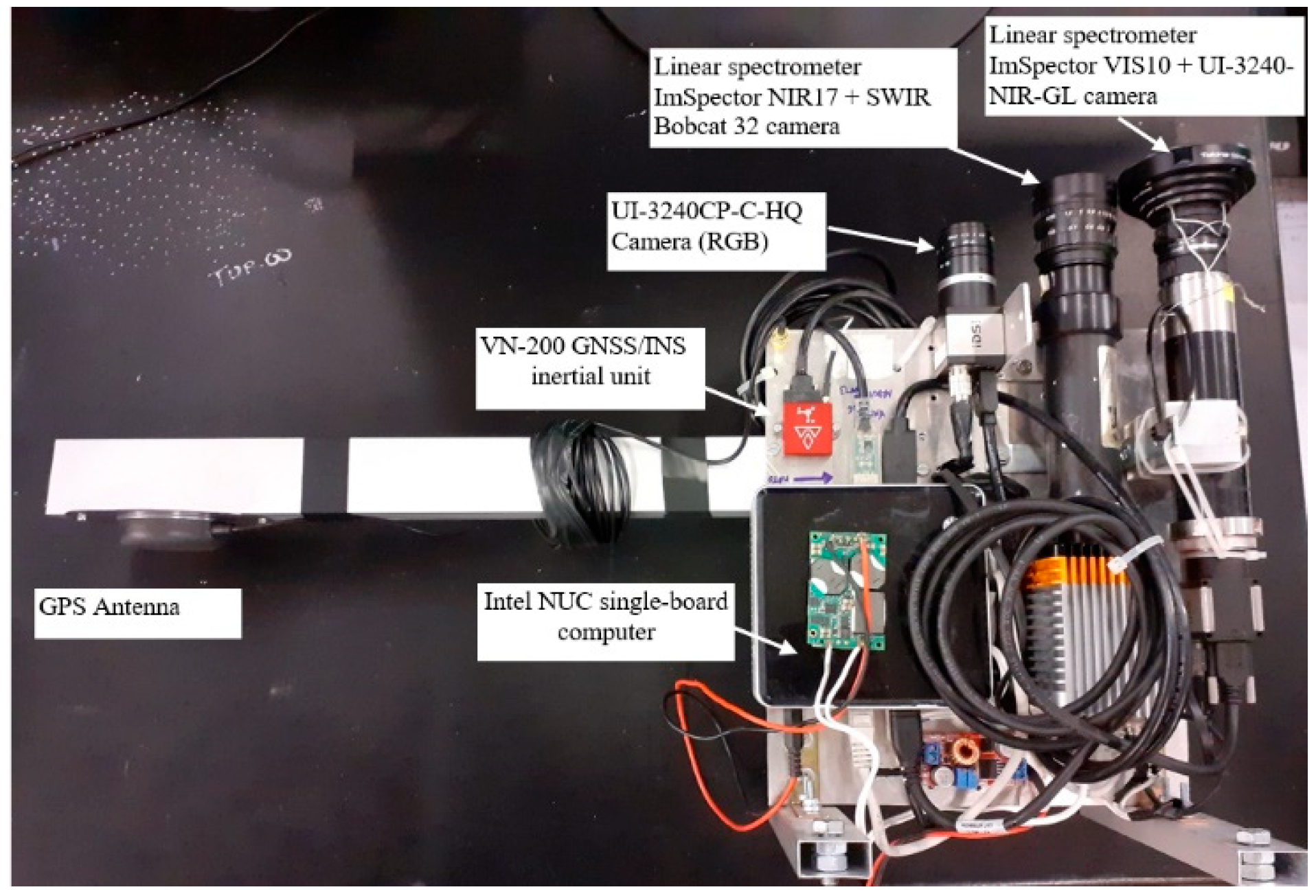
We assembled a stand-alone push-broom hyperspectral sensor system (Figure 1) based on two camera–spectrometer devices operating in the bands 400–1000 nm (VIS/NIR) and 900–1700 nm (SWIR), with the purpose of realizing a stand-alone payload for a relatively small drone covering a large wavelength range for high versatility. While the VIS/NIR sensor is especially useful, e.g., for vegetation monitoring, in this work, we did not use data in that band because we chose to concentrate on the SWIR band that contains narrowband absorption patterns that are specific to plastic polymers. The spectrometer captures a narrow line image of the target through a slit behind the lens and disperses the light from each line pixel into a spectrum, orthogonally, with respect to the line. An Intel-based board PC performed data acquisition and storage, as well as data processing for detection and communication with a ground station. A compact INS provided Global Navigation Satellite System (GNSS)-based geolocation and attitude sensing for hyperspectral cube generation and georeferentiation. An additional RGB camera equipped with a standard lens provided images with strong superposition, adding the option of mosaicking and real-time transmission to the ground of relevant scenes corresponding to alerts.

The SWIR sensor chosen for this project is a Xenics (Leuven, Belgium) Bobcat 320, featuring sensitivity between 900 and 1700 nm (SWIR) and 320 × 256 pixels (easily replaceable by a camera of the same family with 640 × 512 pixels), assembled with a linear spectrometer ImSpector NIR17 OEM by Specim (Oulu, Finland) for capturing light through a narrow slit aligned in the direction of the smaller side of the sensor so that a spectral image of 256 spatial positions × 320 wavelengths (individual bands about 2.5 nm wide) is obtained.

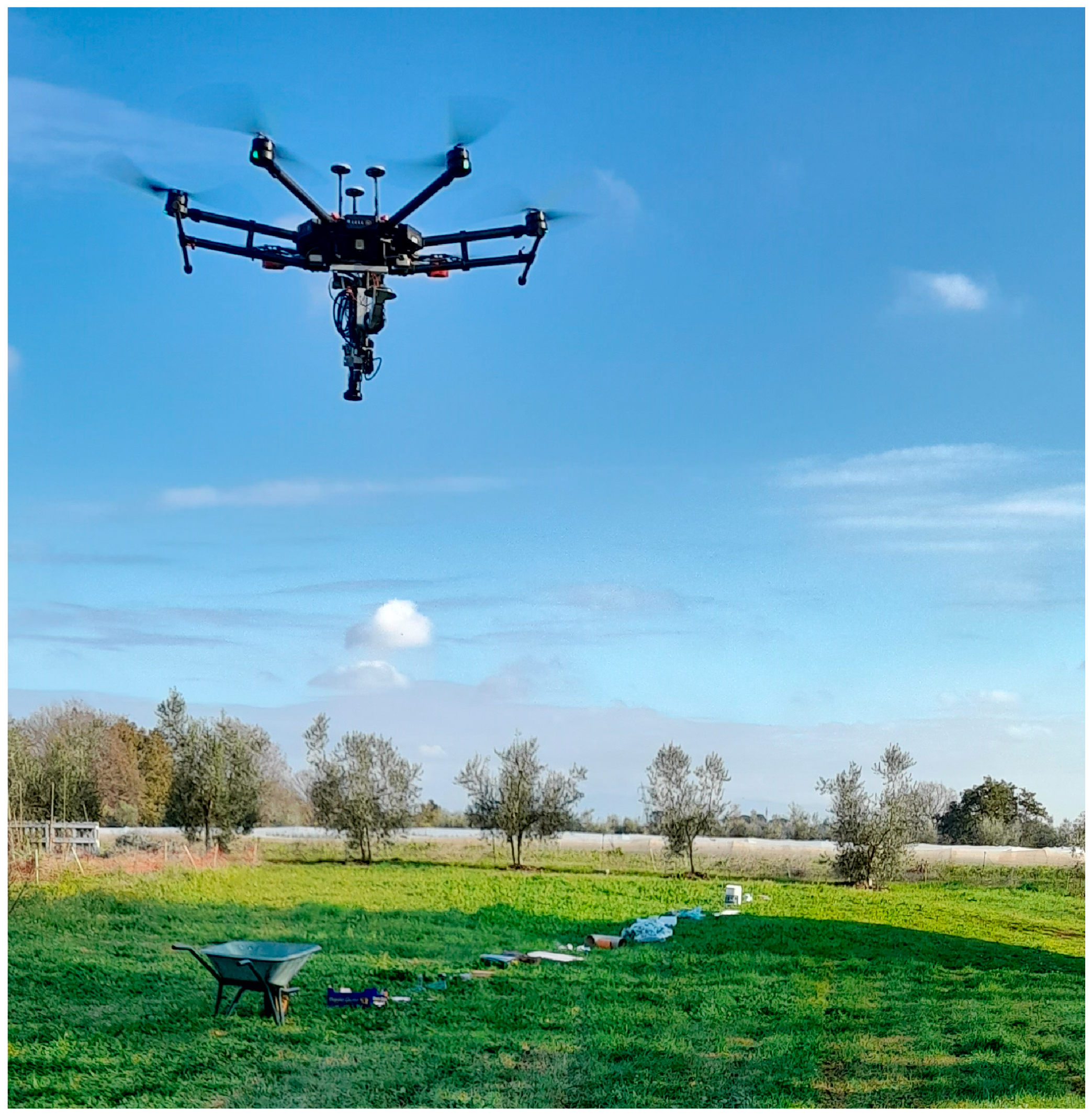
The payload was mounted on a DJI (Shenzen, China) Matrice 600 drone (Figure 2) operated by Oben srl, Sassari, Italy, which was normally flown at 7–15 m height and 0.5–2 m/s speed with an acquisition frequency of 12.5 Hz, obtaining a pixel size (sideways) of 1 to 2 cm.

In order to build the hyperspectral cube, we employ images obtained by a visible camera IDS (Obersulm, Germany) UI-3240-CP-C-HQ synchronized with the other cameras by hardware trigger. A mosaicking algorithm is used to stitch such images together, and the same roto-translation parameters obtained are applied to the spectral images. Such a method proved quite effective and avoided further complication (and cost) of the system, but it occasionally failed on poorly structured surfaces (in particular, over water), and does not allow for georeferentiation of the data. Therefore, in an upgrade of the system, we integrated a Vectornav VN-200 GNSS-aided Inertial Navigation System to provide synchronized position and attitude data for easy and accurate hyperspectral cube reconstruction, as well as to allow for real-time (during flight) georeferenced alerting.

2.2. Data Acquisition

Starting in 2020, we operated the sensor system described above in many diverse survey missions in natural environments, where we placed plastic litter in a controlled manner (partly grouping materials by polymer and holding objects by threads or by sticking them on hidden supports, such as a light fishing net), and/or observing litter already present in the environment, over bare ground or grass, on beaches or river banks, and floating on lake or seawater. The missions were performed in different seasons, in cloudy or sunny weather, and choosing different exposure settings, in order to obtain a diverse database and validate the generalization capability of our algorithms.

In this work, we selected a subset of our database and preferentially employed datasets obtained in controlled conditions for machine learning, where we carefully manually labeled the hyperspectral cubes with ground truth. In particular, the training set we used is extracted from surveys performed in January and March 2020, April 2022, and in two days of February 2024, about two weeks apart from each other. The first two sets were also used for our previous paper on this topic [22], and from the last two surveys mentioned, we selected two cubes each for this work. These cubes will be denoted, respectively, as Jan20, Mar20, Apr22, 7Feb24a, 7Feb24b, 21Feb24a, and 21Feb24b. All these flights, except for 21Feb24b, involved the acquisition of data over grassy or bare ground, where we placed small heaps of plastic objects from normal household waste sorted by polymer type, weathered plastic litter collected on a beach and not sorted, and objects made of other non-plastic materials, such as wood, metal, and glass, as well as some commercial white floor tiles. We observe that detecting plastics on such backgrounds as grassy or bare ground is a more difficult task than detecting objects floating on water because water appears very dark in the SWIR spectrum. Therefore, we assumed that the training set obtained in this way would be most appropriate to also generalize floating objects, provided that they are not fully covered by water. The 21Feb24b survey was taken over a row of tunnel greenhouses, realized with PP transparent foil.

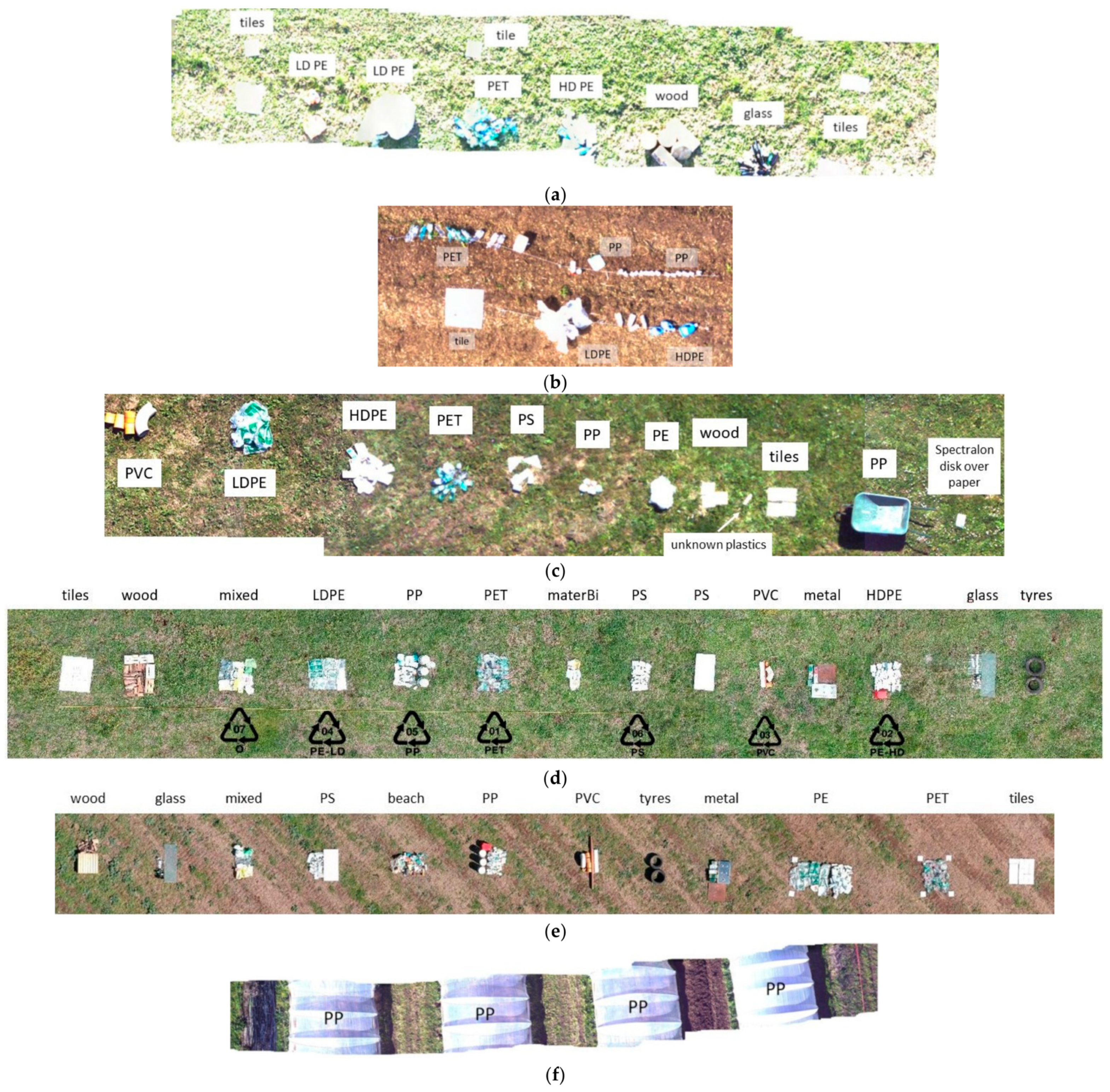
The experimental setup for all surveys is shown in Figure 3.

The single hyperspectral images acquired at the rate of 12.5 Hz have one spatial dimension (linear array of 240 pixels taken across the flight direction), and one wavelength dimension (300 raw bands, downsampled to 81, spaced 10 nm apart from each other). They are stitched together into a hyperspectral cube by appropriate roto-translation so that the so-called cube is, in fact, a parallelepiped with an elongated shape, corresponding to a roughly straight flight path surveying a stripe on the ground. As the single one-dimensional segments are pasted into a matrix that needs to be rectangular in space, along the edges, we fill the cube with blank pixels (the spectra are all set to 0 value). Such blank pixels will be generally represented in gray in the following figures, and are not included in the processing. Of the 81 bands, corresponding to wavelengths from 900 to 1700 nm, the first four (900–930 nm) are empty due to geometrical constraints of the assembly camera–spectrometer. Some bands at the edges and around 1400 nm (the strongest atmospheric water absorption band) were not used for further processing because the data they contain have too low of a level and are therefore strongly noisy. In the end, we used 60 wavelengths in two intervals: 980–1340 nm and 1460–1680 nm.

On the occasion of some of the surveys, we also acquired the spectra of the plastic objects and white tiles using a pointwise spectroradiometer FieldSpec 4 (A.S.D. Inc., Longmont, CO, USA), which measures light intensity in the range of 350–2500 nm. Such acquisitions are calibrated using a Spectralon tile, yielding reflectance across the spectrum rather than absolute sensed power.

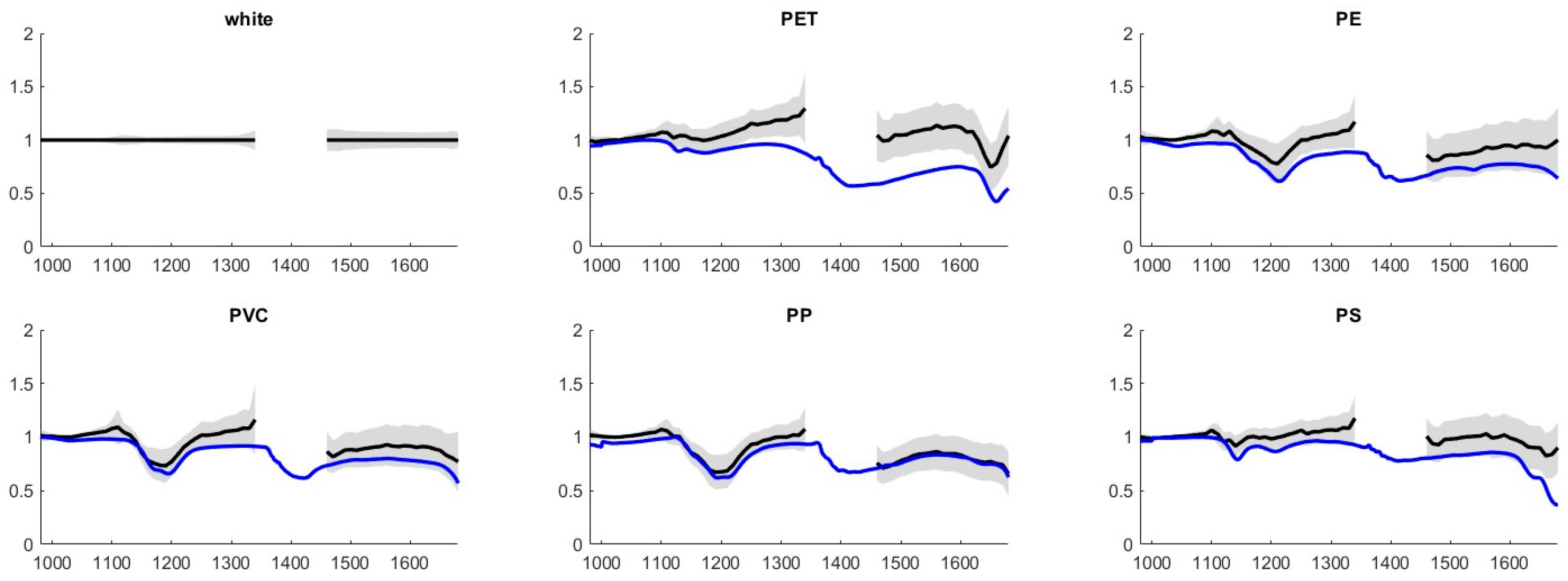
Spectra contained in the 21Feb24a cube used in this work are compared in Figure 4 to the spectra acquired with the spectroradiometer. In order to do this, we calibrated the spectra taken from the drone using the average spectra taken on the white tiles after having checked that the calibrated reflectance of such tiles is quite reasonably flat under the spectroradiometer. In this way, we obtained approximate reflectance for our field data. We also arbitrarily normalized the average spectra for visualization purposes because the purpose of the comparison is to check the agreement in the absorption patterns of the plastic polymers, regardless of absolute reflectance. It is apparent that the spectra acquired from the drone appear quite consistent with the ones acquired with the spectroradiometer, especially observing that the relevant absorption patterns are located at the same wavelengths. We also remark that the variability of the field spectra is reasonably limited so that we may observe that the shape of the spectra is quite consistent across different objects of the same material.

2.3. Methodology for Data Analysis

In this contribution, in continuity with previous work, we apply machine learning (ML). Even if we are also exploring deep learning, we think that the advantage of ML is that it works on a small dataset and that the recall phase requires little computational resources, so it is well suited for embedded implementation in real time.

Following our previous work, in this paper, we also used Linear Discriminant Analysis (LDA) [24] for the classification of individual pixel spectra, implemented with the MATLAB v.24.2 function in its basic form that uses no hyperparameters, and Support Vector Machines (SVM) [25] with RBF (Radial-Basis Function) kernels, optimizing hyperparameters (kernel size and box constraint, i.e., soft-margin width) with the automatic feature of MATLAB to test the possible advantage of nonlinear separating surfaces. In a previous work, we also considered the k-Nearest Neighbors (k-NN) algorithm as a potentially very effective non-parametric algorithm but we did not use it in this work because of its very large computational cost [26]. As we observed previously, it is beneficial to execute feature reduction before learning and applying a classifier because the information contained in the hyperspectral data is possibly redundant, and mainly because some bands contain no information that is useful for the discrimination of materials and contributes noise that may even make the detection more difficult. Also in this work, for this purpose, we used the minimum-redundancy/maximum-relevance criterion (mRMR [27]). We explored in previous work the option of using Principal Component Analysis for feature reduction, finding performance similar to what we obtain with mRMR. However, from a computational point of view, PCA realizes a transformation applied to all bands so that it has a slightly higher computational cost than the straightforward reduction of the number of bands used.

While our previous results [22] proved the efficacy of simple ML algorithms for plastic detection and even for single-polymer discrimination, in the experimental campaigns, we observed that classifiers learned on a given dataset were not always working properly for other datasets, mostly due to changes in exposure settings and shading but also to general environmental conditions (e.g., a sunny or cloudy sky), which caused detection algorithms to perform poorly or fail in some cases. Moreover, working on single cases may cause the algorithm to learn characteristics of the plastic object spectra present in that specific dataset (e.g., brightness) that are not actually significant for plastics with respect to other materials. Such malfunctions make the automation of plastic recognition unreliable and generally prevent the possibility of straightforward real-time operation. For this reason, it is important to use a training set that is representative of diverse environmental conditions and contains different (and, in particular, non-plastic) materials. It is also desirable, if possible, to avoid the necessity of calibration procedures to simplify the deployment of the sensor and the execution of the survey.

Training examples were automatically extracted from the cubes using manually drawn templates that identify the following:

• Six plastic classes: PET, PE (both LDPE and HDPE grouped together), PVC, PP, PS, and other plastics (those currently identified with code 7, including bio-based plastics and mixed materials, as well as groups of mixed objects that were not sorted by polymer);
• One class for white reference objects (white commercial floor tiles, which we verified with a point spectrometer as being satisfactorily white in the SWIR spectrum);
• One class for non-plastic objects;
• One class for background (generally grass, or occasionally bare earth).

In each hyperspectral cube, we extracted 100 samples per class, except 300 samples each for non-plastics and background. Taking into account that some polymers (and also non-plastic objects) are not present in all samples, we took a total of 7300 samples, reduced to 6350 after eliminating all the spectra that were too dark (average < 32 DN after dark current level removal, in a range of 256). Such samples were simply chosen by extracting evenly spaced samples from the arbitrarily ordered list of all samples belonging to each class in the cube (as indicated by manually drawn labeling templates). In the same way, we also extracted a test set, just displacing the new sequence of evenly spaced samples as much as possible from the one used for the training set.

We considered the following training cases:

• All plastics: namely, all six plastic classes combined into a positive class, and everything else in the negative class (600 positive, 700 negative samples from each cube that had all classes);
• One polymer vs. non-plastics: namely, one of the five identified polymers (excluding the mixed plastics class) in the positive class, the other plastic classes in a “don’t care” class (i.e., excluded from the training set altogether), and the non-plastics and background classes combined into the negative class (100 positive, 700 negative samples);
• One polymer “only”: namely, one of the five identified polymers in the positive class, and the other plastic classes (leaving the “mixed” one as “don’t care”) together with the non-plastic and background classes in the negative class (100 positive, 1100 negative samples).

The case “all plastics” is directly relevant to the detection of plastic litter in the environment, where it is not necessary to distinguish among different plastic polymers; the case of one polymer vs. non-plastics is also relevant to the same situation because binary classifiers for single polymers (whose results may be combined in logical OR to obtain all plastics) may be more effective than a single classifier generalizing all plastic polymers at once that have different absorption patterns. Leaving other polymers as “don’t care” relaxes the constraints for the classifiers so that they may give positive outcomes on other polymers without this being a problem when the various outcomes are then combined. The case of one polymer only (vs. other polymers, besides non-plastics) is definitely relevant to the application of polymer sorting in recycling facilities but is also interesting to consider in this context because, in some cases, it may perform better than the “don’t care” approach described above.

Since the training sets are generally unbalanced between positive and negative classes, as a performance parameter, we chose Cohen’s Kappa coefficient [28].

Indicating true-positive (negative) and false-positive (negative) outcomes as TP (TN) and FP (FN), respectively, and the number of examples as N, we compute

Accuracy = (TP + TN)/N

(1)

ExpectedAccuracy = ((TP + FP) × (TP + FN) + (TN + FP) × (TN + FN))/N²

(2)

Kappa = (Accuracy − ExpectedAccuracy)/(1 − ExpectedAccuracy)

(3)

Kappa essentially coincides with the Matthews Correlation Coefficient (MCC) for relatively high values (i.e., when performance is not bad) and seems more widely used in the literature than MCC. It gives a fair score of performance even with unbalanced classes by evaluating the improvement over expected accuracy, i.e., the accuracy that would be obtained by assigning outcomes totally by chance.

3. Results

We started with a series of experiments aimed at optimizing choices about the machine learning algorithm and the feature selection strategy. In our previous paper [20], we already discussed such issues, and here, for further validation, we repeated the analysis specifically on the selected hyperspectral cubes, initially executing training and testing (on different sets of examples) on the same cube for each one of them.

As an example, the results of such an experiment are reported for the 21Feb24a dataset. The Kappa scores are listed in

Table 1. Kappa score for LDA classification of 21Feb24a data.

# Features	All	PET	PET Only	PE	PE Only
10	0.54	0.94	0.83	0.84	0.23
15	0.58	0.94	0.83	0.88	0.54
20	0.64	0.95	0.84	0.9	0.51
25	0.83	0.96	0.84	0.9	0.54
30	0.87	0.96	0.87	0.91	0.59
35	0.89	0.95	0.91	0.93	0.56
40	0.89	0.95	0.91	0.91	0.60
50	0.90	0.95	0.91	0.92	0.62
60	0.90	0.96	0.9	0.92	0.62

and

Table 2. Kappa score for SVM classification of 21Feb24a data.

# Features	All	PET	PET Only	PE	PE Only
10	0.82	0.95	0.83	0.84	0.64
15	0.85	0.95	0.83	0.94	0.63
20	0.87	0.96	0.83	0.94	0.50
25	0.92	0.96	0.87	0.94	0.70
30	0.92	0.96	0.84	0.96	0.71
35	0.94	0.96	0.88	0.95	0.69
40	0.95	0.96	0.89	0.96	0.70
50	0.96	0.95	0.88	0.96	0.65
60	0.96	0.97	0.87	0.95	0.66

for LDA and SVM, respectively, for several numbers of features selected by mRMR. Classification is executed for all plastics (i.e., the union of the six plastic classes mentioned above) and for PET and PE (the polymers that were present in six out of seven cubes), with other polymers in the “don’t care” or in the negative classes (the latter denoted with “only”). The results for other polymer classes and other cubes are similar and not reported here for conciseness.

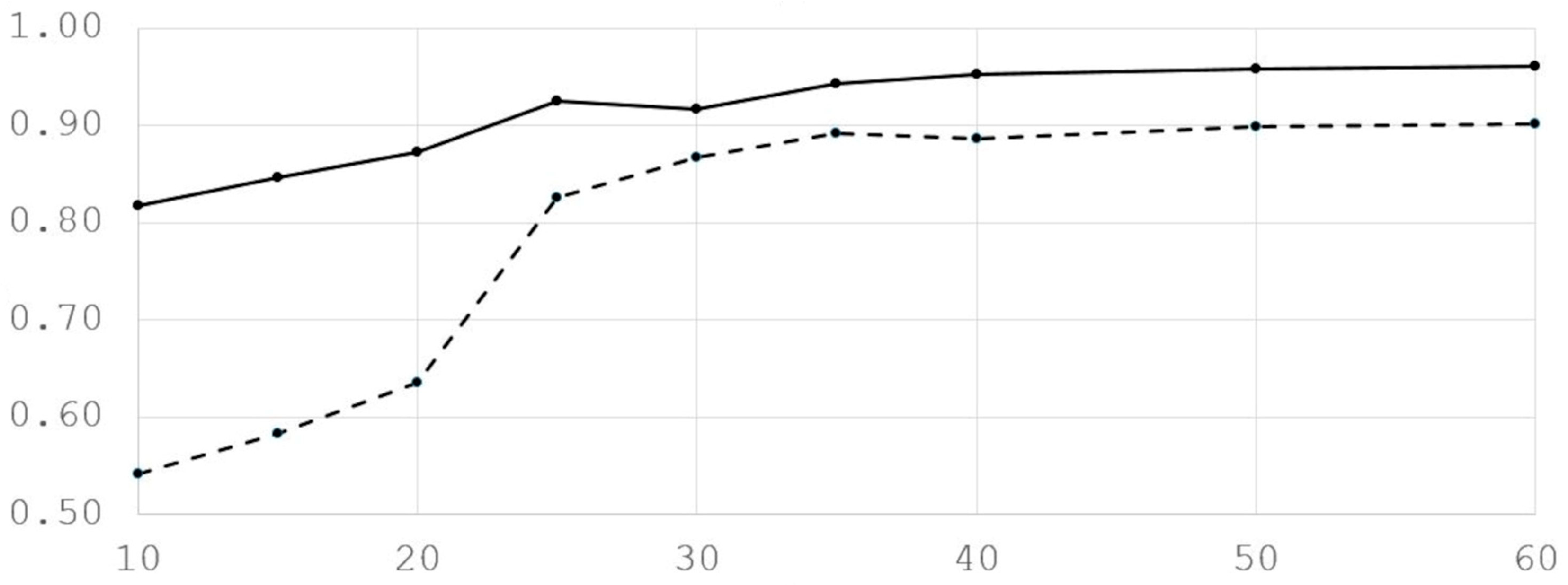
Figure 5 shows the Kappa score for the classifiers for all plastics. It is apparent that upon increasing the number of features selected, the Kappa score increases, saturates, and then possibly eventually slightly decreases. This is expected because the least significant features only add noise into the dataset, without providing additional information.

This example shows typical behavior as also observed in the other datasets and for the detection of the other polymers. SVM generally performs better than LDA; however, we continued using LDA, too, because it is computationally less expensive and because it generally does not perform significantly worse than SVM, sometimes even yielding better results. Indeed, the computation time of the SVM in MATLAB appeared to be almost quadratic in the number of support vectors in our experiments. Models with about 100 support vectors gave a computation time that was almost equal to LDA, but the largest model (1618 support vectors) requires about 80 times as much time compared to LDA. This means that a small kernel size should be avoided.

In the following, we will use the 30 best mRMR features because this is approximately the typical value where saturation of performance begins to appear.

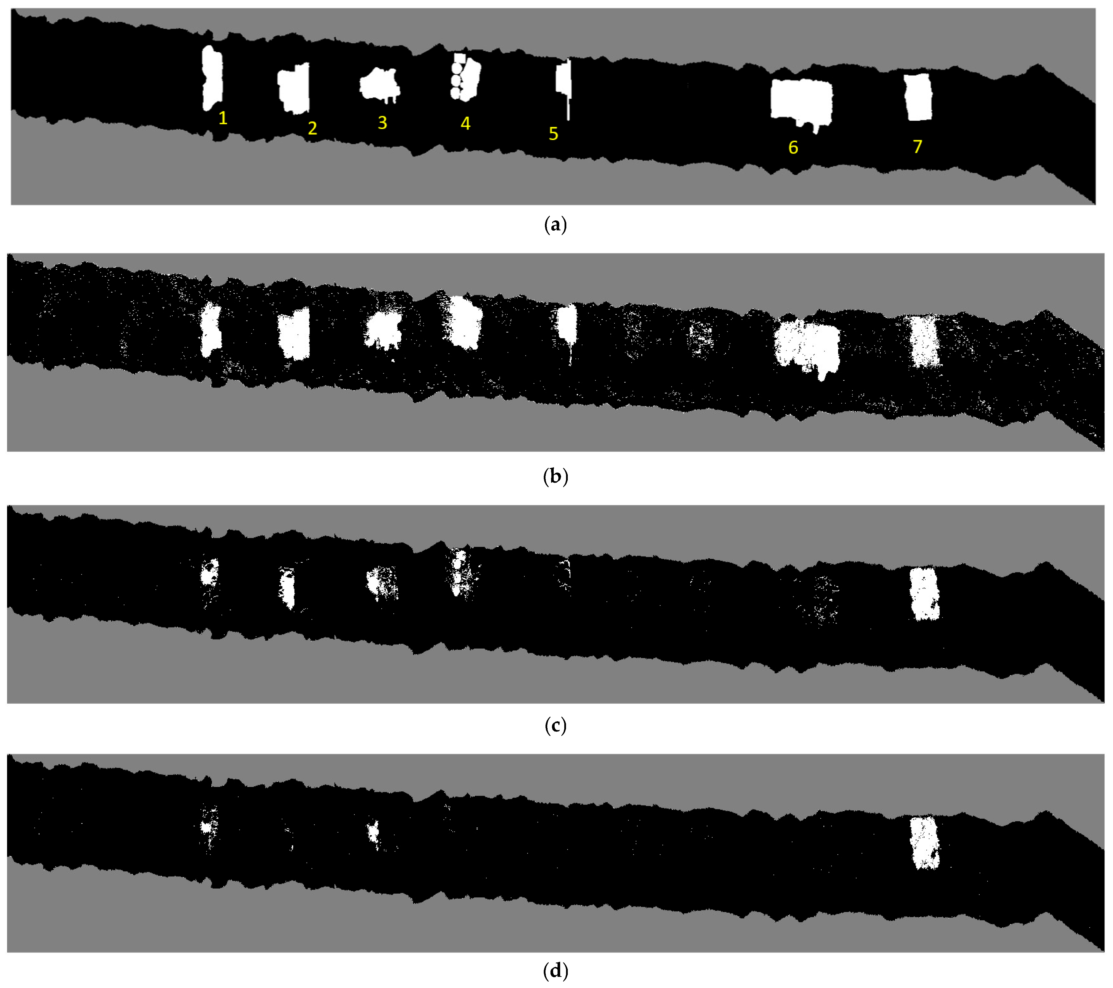
The materials distribution for the case considered is visible in Figure 3e. Please take into account that the footprint on the ground of the visible image is not equal to the one of the hyperspectral cube and that they are not co-registered. In fact, Figure 3 is obtained from a mosaic of a few high-resolution images, optimized for presentation only.

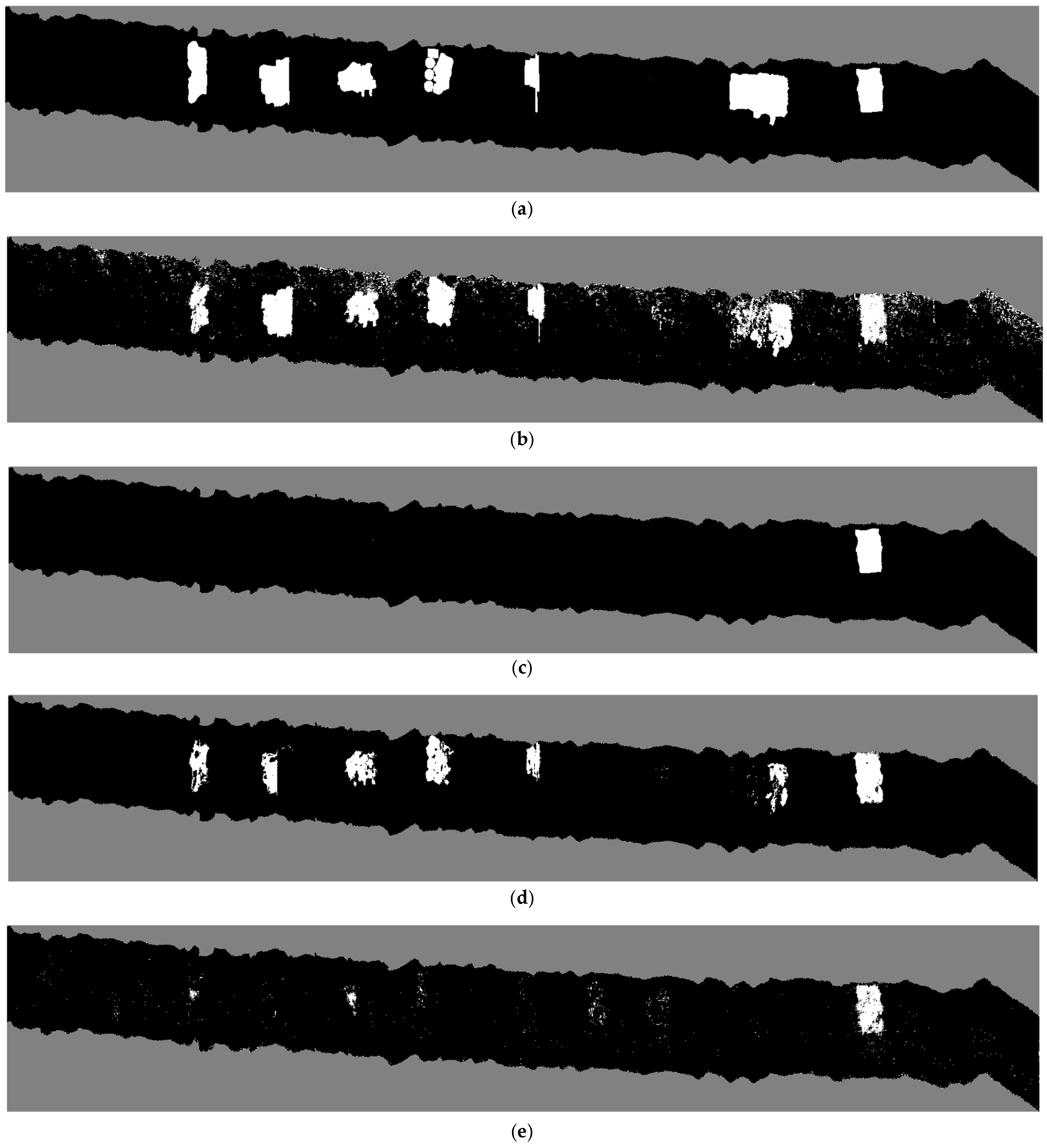
Figure 6 illustrates the application of the SVM classifier, trained on 30 features, to the classification of all plastics, PET (“don’t care”), and PET only for the 21Feb24a cube. Especially, observing the results for all plastics, we notice several isolated false alarms that should be filtered out by morphological operators or rank filters. The results obtained on single polymers show significantly fewer false positives. For this reason, applying classifiers for single polymers (or sub-groups of polymers that have similar absorption patterns) and then combining results in logic OR may yield better overall results for the detection of all plastics at once. Moreover, it is to be noted that isolated false positives could disappear by processing pixels in their local context, either feeding a small window around the current pixel into an ML classifier or using explicitly convolutional schemes, in a higher-rank LDA or SVM model or in deep learning. As expected, the classifier for PET trained with the “don’t care” option also gives positives on other polymers. The classifier trained for “PET only” also responds in some areas other than the one indicated in the desired output. This is not due to false positives and is, instead, correct. In fact, those areas are contained in the “mixed” classes (including weathered objects collected on a beach), where samples of PET objects are indeed present.

In order to choose the most appropriate adjustment of the spectra with the purpose of generalization across datasets, we tried the following options:

• Simple level adjustment: After observing that no features that are especially significant for plastic detection are present in the lowest part of the SWIR wavelength range, we chose to divide each spectrum by the value at 1030 nm to make the overall levels more similar. This is computationally the fastest option considered, and we further observed that using the mean across the spectrum, or only in the lower band, or even applying the z-score (centering and normalization by the standard deviation), does not change performance significantly (we do not report details of the latter alternatives here, for simplicity);
• Calibration using white reference: The mean spectrum of training examples taken on the white reference tiles is used as a divider, wavelength by wavelength, for all other spectra. Such an operation may amplify noise in bands where solar radiation at the ground level is weak. It is to be noted that using calibration implies a procedure to be executed on the field at each survey, which should be avoided if possible.
• Calibration and subsequent level adjustment;
• Continuum removal. Such a type of spectrum pre-processing is quite popular in hyperspectral data exploitation [29] and is meant to make the absorption peaks most evident. In our case, we adjusted the method by fixing a priori which wavelengths are fixed at 1, after checking the typical spectra of plastic and non-plastic material, avoiding constraining wavelengths that are close to where plastic polymer absorption typically happens [30]. This methodology is the most computationally intensive among those considered in this paper.

We tried training on three cubes (for the “all plastics” case), namely 7Feb24a, 21Feb24a, and Apr22a, and testing on each one separately using the above-mentioned normalization methods; thus, we obtained the scores listed in

Table 3. Average Kappa score for the SVM classifier trained on three datasets and tested on each one separately.

	Raw Spectra	Level Adj.	Calibration	Calib. + Level Adj.	Continuum
21Feb24a	0.64	0.88	0.87	0.87	0.87
7Feb24a	0.86	0.82	0.80	0.81	0.77
Apr22	0.88	0.85	0.88	0.83	0.84
average	0.79	0.85	0.85	0.84	0.83

. It is to be noted that calibration was only possible when we had a clearly readable white reference, realized by a large square of white tiles.

Indeed, applying normalization techniques clearly improves performance over results obtained on the raw cube. It is also apparent that simple level adjustment performs generally better, or at least not worse, than the other methods, and is definitely simpler in application, requiring just division by a single value of each spectrum.

In order to verify the potential of generalization across different datasets, we tried a leave-one-out (LOO) procedure by using composite training sets to collect six of the seven datasets—testing on the seventh—in all seven possible combinations (

Table 4. Average Kappa score for LDA classification. LOO procedure on seven datasets. Please notice that the 21Feb24b cube does not contain any PET or PE. Cube 21Feb24b does not contain any PET or PE, therefore corresponding cases are not applicable (N/A).

Tested on	All	PET	PET Only	PE	PE Only
Jan20	0.26	0.68	0.39	0.70	0.65
Mar20	0.29	0.00	0.01	0.54	0.63
Apr22	0.66	0.02	0.41	0.38	0.08
7Feb24a	0.39	0.65	0.60	0.72	0.67
7Feb24b	0.14	0.35	0.56	0.53	0.30
21Feb24a	0.47	0.91	0.81	0.77	0.61
21Feb24b	0.88	N/A	N/A	N/A	N/A

).

This experiment shows that in most cases, the classifier learned on different cubes also works reasonably well on a cube that was not included in the training. Even Kappa values of the order of 0.3 indicate a generally successful detection if considered on groups of pixels rather than single ones, as commented above. A few cases fail (e.g., PET for Mar20 and Apr22, “PET only” for Mar20) or have poor performance (all plastics for 7Feb24b). While this can be in part attributed to inaccurate ground truth reference (in particular, for the Mar20 and Apr22 cubes, which contained some scattered objects and were difficult to accurately identify manually while drawing the label masks), these shortcomings also indicate that the environmental conditions and sensor settings must be controlled carefully to obtain uniform and good-quality data.

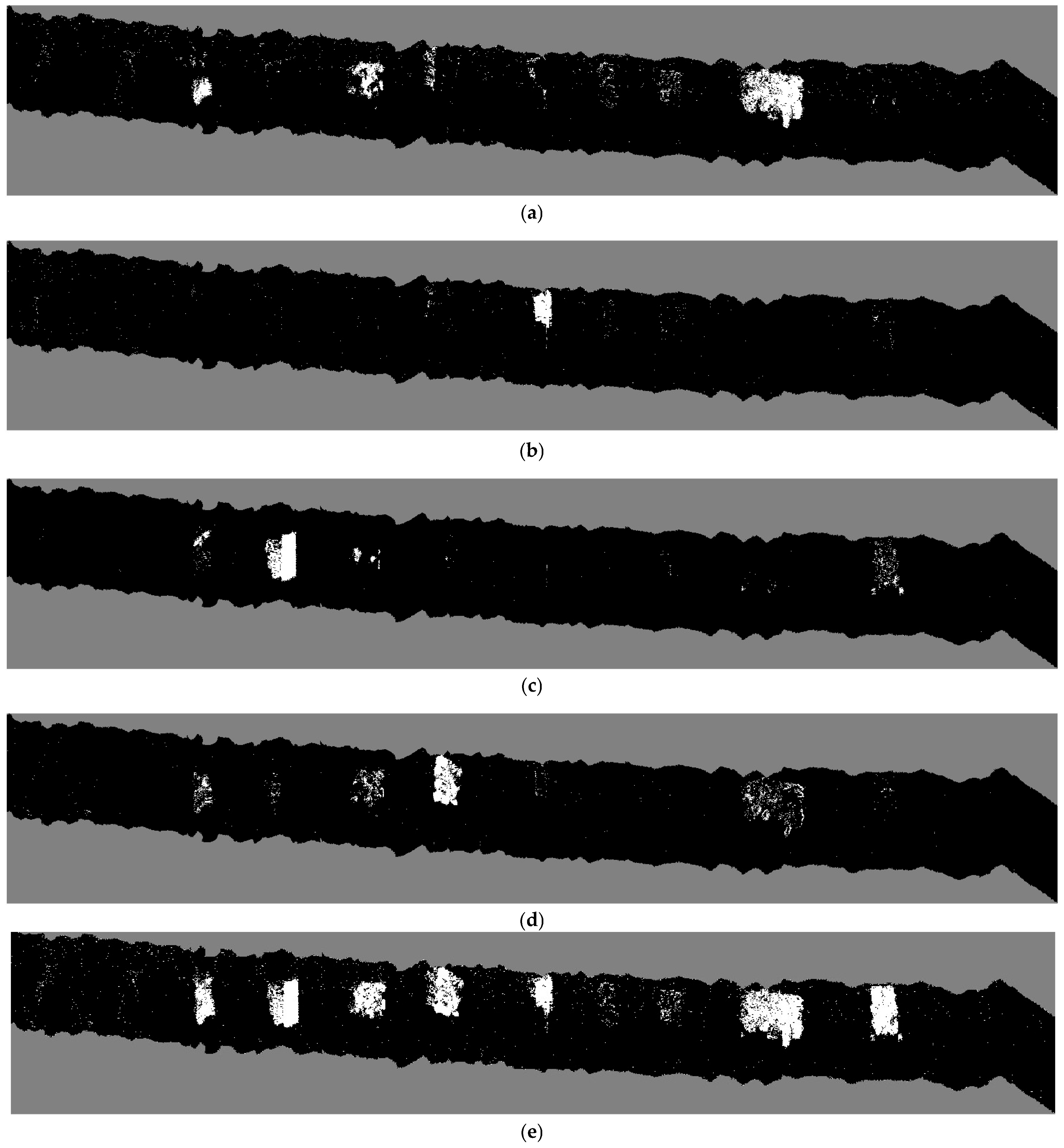
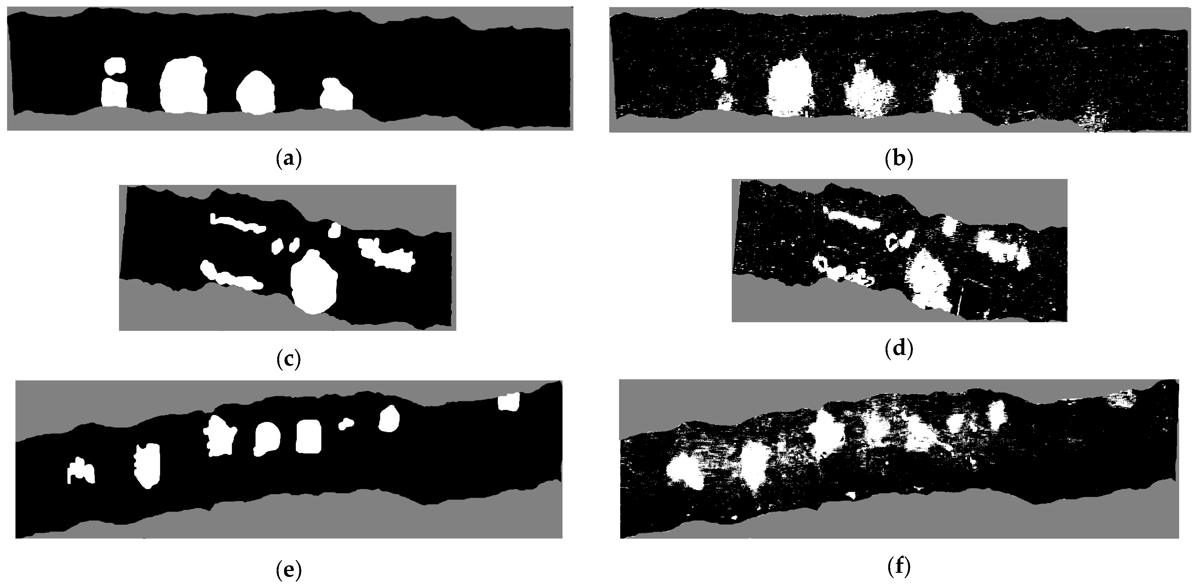
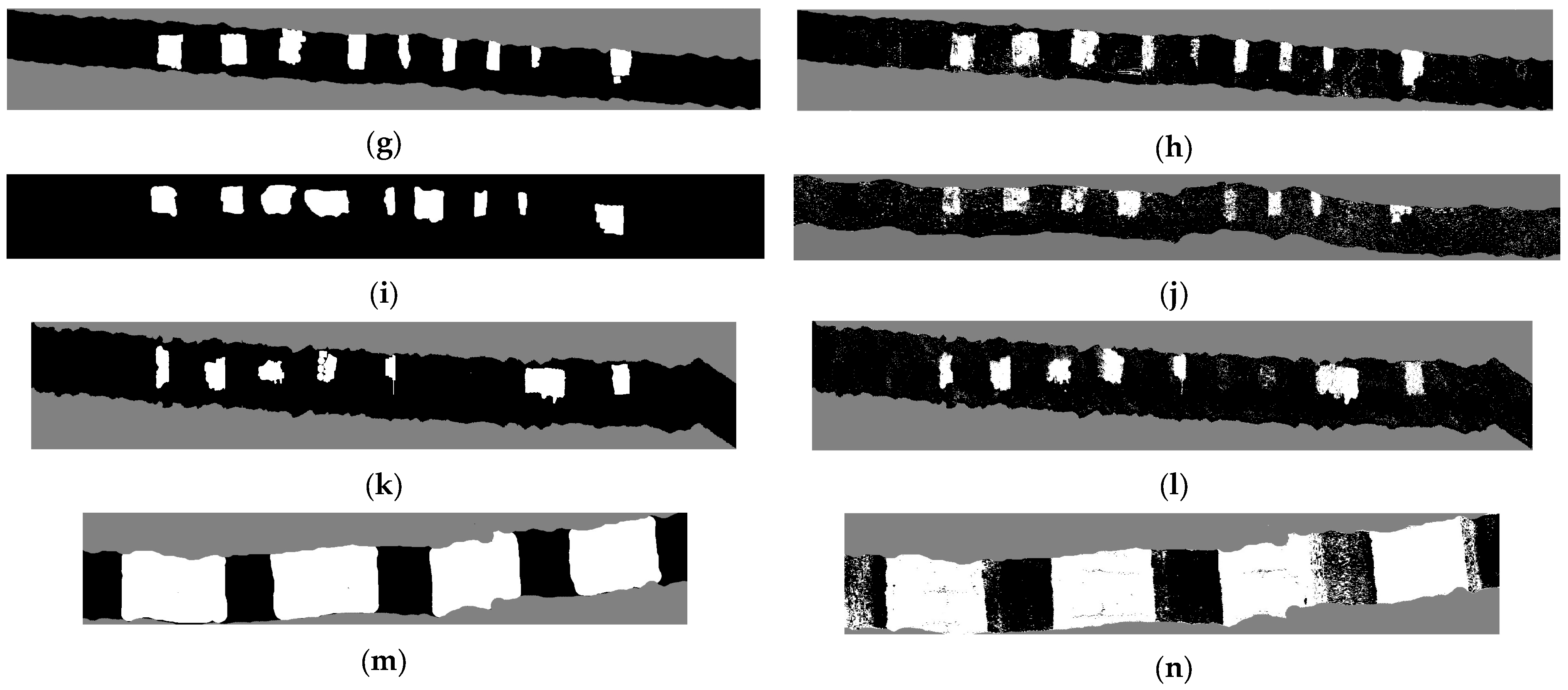
Examples of results using the SVM classifier obtained with simple normalization are shown in Figure 7 (for some polymers) and Figure 8 (for the others). Figure 8e, compared with Figure 7b, shows that combining the results for single polymers in logical OR yields cleaner results than using a single classifier for all plastics.

Table 5. Kappa score for SVM classification trained on seven cubes with simple level adjustment. Some cubes do not contain all polymers (cells indicated as N/A).

Tested on	ALL	PET	PETonly	PE	PEonly	PS	PSonly	PVC	PVConly	PP	PPonly
Jan20	0.85	0.93	0.88	0.80	0.77	N/A	N/A	N/A	N/A	N/A	N/A
Mar20	0.78	0.80	0.71	0.83	0.84	N/A	N/A	N/A	N/A	0.77	0.69
Apr22	0.86	0.83	0.84	0.91	0.92	0.79	0.46	0.95	0.95	0.81	0.77
7Feb24a	0.81	0.80	0.73	0.86	0.88	0.83	0.44	0.97	0.95	0.89	0.79
7Feb24b	0.61	0.63	0.64	0.61	0.46	0.67	0.36	0.99	0.98	0.44	0.33
21Feb24a	0.92	0.95	0.94	0.96	0.82	0.95	0.58	0.95	0.91	0.96	0.80
21Feb24b	0.90	N/A	N/A	N/A	N/A	N/A	N/A	N/A	N/A	0.94	0.90

shows Kappa scores (computed on the test sets) for the SVM classifiers trained on all seven cubes and applied to each of them for all plastic classes. It is apparent that the performance is quite satisfactory in all cases.

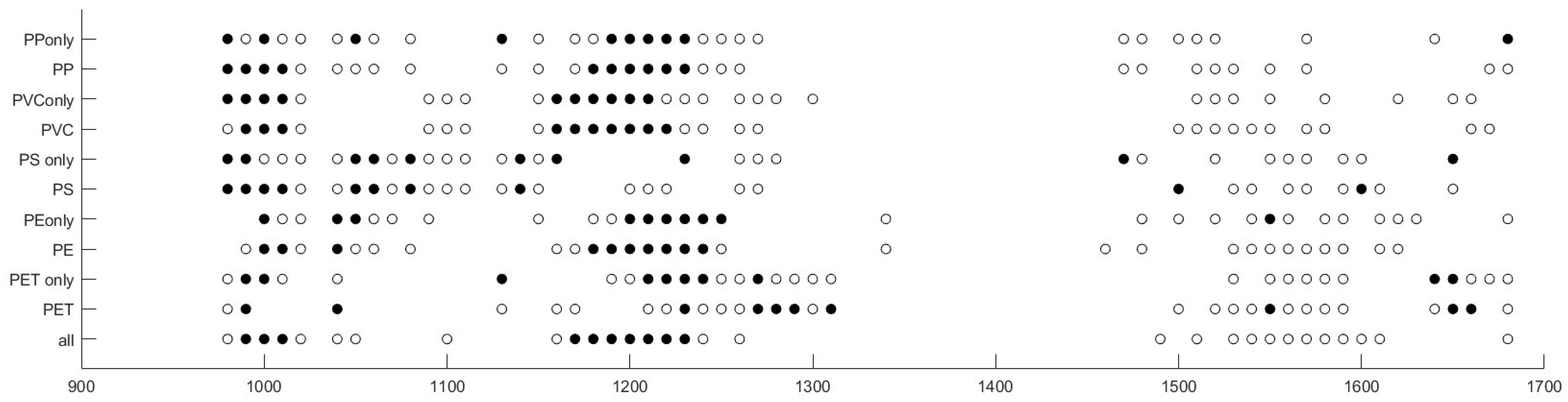
Figure 9 graphically indicates which wavelength features were selected by mRMR. Filled circles indicate the first 10 features ranked, and empty circles indicate the other 20. The wavelength distribution of the most significant features may be compared to the position of the specific absorption peaks observable in Figure 4, taking into account that from a mutual information point of view, the relative response at different wavelengths is also relevant [30], so that not only absorption peaks contribute to the result.

Figure 10 shows the results of the application of the SVM classifiers for “All plastics”, trained on seven cubes, for each one of them. Such results qualitatively prove the generally good performance of the methodology proposed.

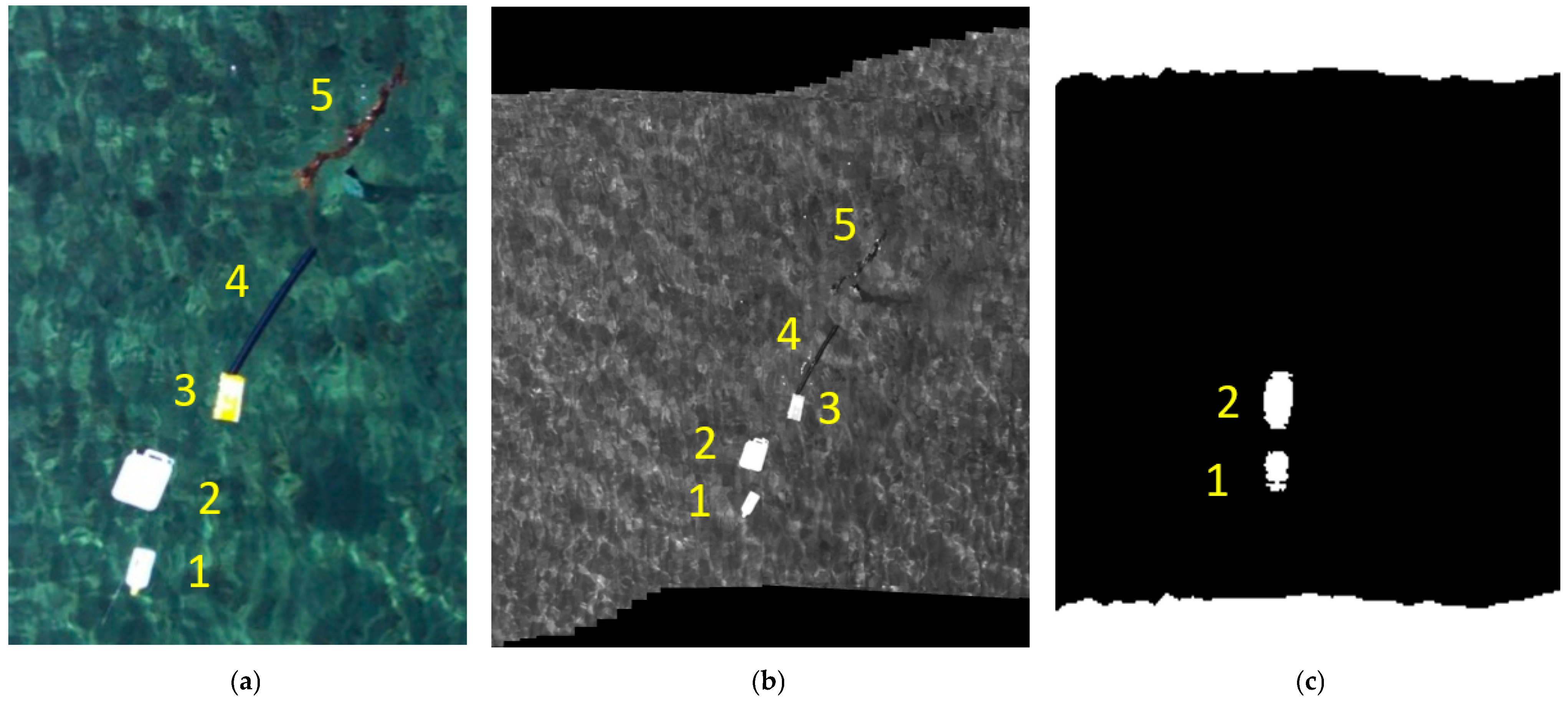
As a further confirmation of the generalization capabilities of the methods and algorithms optimized in this work, we report here the result on one case of objects floating in seawater near the beach, a dataset we already presented in our previous paper [22]. In Figure 11, we may observe that the classifier for all plastics correctly recognizes the plastic objects, distinguishing them from the others.

4. Discussion and Conclusions

In this study, we present an embedded, drone-based hyperspectral survey system enhanced by classical machine learning methods to detect plastic waste in diverse environments. The experiments show that this setup adapts well to changing environmental conditions without requiring calibration or retraining. Below, we summarize the key advances over our earlier studies, address the feasibility of real-time operations, and discuss potential future directions involving deep learning.

In prior work, we relied on single-site training and testing, which limited transferability. In contrast, this present study integrates data acquired in various flights and systematically evaluates the classifiers’ performance in unfamiliar environments. The results confirm that relatively simple normalization procedures, such as dividing each spectrum by the reflectance at 1030 nm, can mitigate exposure and lighting inconsistencies, without requiring site-specific calibration.

A notable strength of the proposed technique is its modest computational overhead at the inference stage. Although hyperspectral data can be high-dimensional, the use of feature-selection strategies (mRMR) combined with efficient classifiers (LDA or SVM) ensures that real-time execution on a drone platform is feasible. This becomes particularly relevant for aerial surveys where hardware and power constraints are stringent. Future work might focus on optimizing or parallelizing the algorithmic components—potentially with GPU-based processing—to achieve even faster detection in real-time scenarios.

In this work, we essentially assumed that plastics essentially occupy entire pixels, based on the fact that the pixels of our cubes are indeed very small, and also exploiting the fact that our scenarios mostly include patches of objects made of the same material. We plan to investigate the detection of plastics occupying pixels only in part (and possibly in low density) when we proceed to use satellite data and when considering scenarios where small objects are widely scattered. This is an important issue that we will deal with in future work.

While this study primarily employs classical ML, deep learning (DL) techniques offer possibilities for further refinement:

• Spectral–spatial convolution: convolutional neural networks (CNNs) could harness both the spectral signatures and spatial structure of hyperspectral cubes, potentially reducing false alarms and improving the localization of plastic debris;
• Automatic feature exploitation: DL models can learn discriminative features directly from raw data, reducing or eliminating the need for feature selection.

Nevertheless, several challenges arise when implementing deep learning:

• Data requirements: CNNs demand large training sets. Gathering sufficient labeled data may be difficult, and overfitting may occur without adequately diverse training data.
• Computational complexity: deep networks typically require considerable computational power, which might not be available in embedded solutions.

The continuation of this work will concentrate on executing surveys in a wider range of case studies, with specific attention to real situations where plastic litter is dispersed or accumulated in the environment, both on the ground and in the water. From an algorithmic point of view, context information will be integrated into the ML algorithm, and other learning systems capable of embedded implementation will be applied.

Data fusion with satellite surveys will also be considered in order to attempt spatialization of the small-area accurate detection obtained from a drone or airplane by employing large-area multispectral or hyperspectral satellite data in a synergic approach.