Abstract
Woody plants serve as crucial ecological barriers surrounding oases in arid and semi-arid regions, playing a vital role in maintaining the stability and supporting sustainable development of oases. However, their sparse distribution makes significant challenges in accurately mapping their spatial extent using medium-resolution remote sensing imagery. In this study, we utilized high-resolution Gaofen (GF-2) and Landsat 5/7/8 satellite images to quantify the relationship between vegetation growth and groundwater table depths (GTD) in a typical inland river basin from 1988 to 2021. Our findings are as follows: (1) Based on the D-LinkNet model, the distribution of woody plants was accurately extracted with an overall accuracy (OA) of 96.06%. (2) Approximately 95.33% of the desert areas had fractional woody plant coverage (FWC) values of less than 10%. (3) The difference between fractional woody plant coverage and fractional vegetation cover proved to be a fine indicator for delineating the range of desert-oasis ecotone. (4) The optimal GTD for Haloxylon ammodendron and Tamarix ramosissima was determined to be 5.51 m and 3.36 m, respectively. Understanding the relationship between woody plant growth and GTD is essential for effective ecological conservation and water resource management in arid and semi-arid regions.
1. Introduction
Arid and semiarid regions occupy 41% of the global land area and support more than 38% of the global population [1]. Over the past 60 years, these regions have continued to expand and caused widespread water scarcity [2,3]. Global warming, along with decreased precipitation and increased evaporation, may further reduce the availability of water resources in arid and semiarid regions [4]. Rapid population growth and socio-economic development, along with rising anthropogenic water demand, are exacerbating water scarcity in these regions [5]. Consequently, the contradiction between ecological water consumption and anthropogenic consumption is intensifying. In this context, natural deserts, which serve as important ecological barriers, continue to deteriorate in arid and semi-arid regions [6]. This degradation poses a potential ecological crisis, threatening local livelihoods, production and the stability of the internal oasis ecosystem. Therefore, monitoring the vegetation distribution in desert ecosystems and assessing its responses to climate change and human activities are essential for maintaining ecological security and improving ecological services in these regions.
Approximately 23% of the world’s deserts are temperate deserts, with 80% of these located in Central Asia [7]. These regions are also an important part of the global groundwater-dependent system (GDEs) and are of greatest concern in arid regions [8]. Generally, woody plants in temperate deserts consist of shrubs (e.g., xerophytic or ultraxerophytic shrubs, semi-shrubs) and small trees. These plants are important ecological barriers preventing desertification from invading the overall oasis systems. With limited precipitation and atmospheric condensation, woody plants in arid and semi-arid regions can flexibly utilize shallow, middle or deep soil water, as well as groundwater. However, the degradation of woody plants is often subtle and may exhibit a lag effect. Once damage occurs, natural recovery is slow or even irreversible, which threatens the stability and survival of oases [9]. Recently, the relationships between the growths of woody plants and groundwater table depths (GTD) have been reported in inland river basins (e.g., Heihe, Sangonghe River and Tarim River) [6,9,10,11]. Most vegetation information (e.g., coverage, density, height) has been obtained from ground sampling. Due to the uneven spatial distribution of woody plants, however, limited sampling data cannot accurately characterize the distribution and structure of vegetation across these regions.
Woody plants in arid and semiarid regions usually have low coverage and high heterogeneity [6]. Their vegetation growth can be obtained from a long-term series of medium- and low-resolution remote sensing images, but the accuracy of woody plant mapping is relatively low due to the interference of mixed pixels. In recent years, with the continuous increase in domestic Gaofen (GF) series remote sensing data sources, it has been widely used for vegetation mapping of forests, grasslands, wetlands, cropland, deserts and other ecosystems [12,13,14]. With the continuous development of deep learning technology, many models (e.g., D-LinkNet model, FCN8S model, DeepLab model) have been widely used in forest mapping [15], cropland mapping [16], land use and land cover mapping [17]. The D-LinkNet model was originally developed for road detection based on high-resolution images, especially for the extraction of discontinuous roads that were obscured by shadows from trees and buildings [18]. As it can avoid losing many details in the subsampling process, and is more suitable for the extraction of discontinuous, sparsely distributed or borderless objects. Therefore, combining high-precision GF satellite and multi-temporal Landsat satellite images can improve vegetation index products for woody plants in desert regions over a long time-series.
Firstly, based on machine learning methods, it utilizes Gaofen-2 remote sensing data to accurately extract the spatial distribution of woody plants, and combines it with Landsat data to construct a long time-series vegetation indices product. Secondly, it develops a fine indicator for delineating desert-oasis ecotone based on the difference between fractional woody plant coverage (FWC) and fractional vegetation cover (FVC). Finally, it analyzes the relationship between vegetation growth and groundwater table depth (GTD) across different ecohydrological zones and estimates the ecologically optimal water levels for two woody plants.
2. Materials and Methods
2.1. Study Area
The Sangong River Basin (SRB) is situated in the middle of the northern slope of the Tianshan Mountains, adjacent to the southern edge of the Gurbantunggut Desert (44°07′N-44°31′N, 87°41′E-88°13′E). It has a temperate continental climate, with an annual temperature of 6.6 °C, annual precipitation of 160 mm, and annual pan evaporation ranging from 1533 to 2240 mm [18]. This study focuses on the middle and lower reaches of the SRB, where the main landscape types are oases and deserts. The temperate deserts here have unique geographical and hydro-ecological characteristics, making them a typical example for studying the relationship between woody plants and groundwater. From south to north, it can be divided into four ecohydrological regions: the ADFO (alluvial-diluvial-fan oasis), APOU (alluvial-plain oasis, upper), APOL (alluvial-plain oasis, lower) and desert (the northern desert) regions (Figure 1a) [19]. The GTD reaches up to 70 m in the upper upstream regions near the mountains, but ranges between 5 and 10 m in the lower reaches near the deserts (Figure 1b). River runoff here is mainly supplied by snowmelt water, and almost all of it is retained in upstream reservoirs, resulting in no surface runoff into the northern desert region.
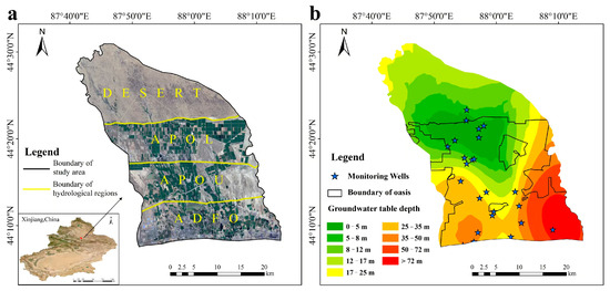
Figure 1.
(a) represents the location of the study area, (b) represents groundwater contour maps.
Haloxylon ammodendron (H. ammodendron) and Tamarix ramosissima (T. ramosissima) are two of the dominant woody plants here. Most of the T. ramosissima distributed in the periphery of the oasis have been reclaimed for cropland, while large quantities of H. ammodendron are still preserved in the northern deserts [20]. The snowmelt water, precipitation, soil water and groundwater are the main water sources of these two plants here. Crops and shelterbelts in the oasis mainly rely on channel-transported water and groundwater pumping.
2.2. Data Sources
2.2.1. Remote Sensing Images
In this study, we selected 4 scene GF-2 images acquired in July 2021 and 1 scene GF-2 image acquired in August 2021 from the China Centre for Resources Satellite Data and Application “https://www.cresda.com/” (accessed on 22 December 2022). We used ENVI software (v 5.3) to carry out radiometric correction, atmospheric correction, orthographic correction, image mosaicing and fusion on Gaofen-2 images and finally obtained four-band images with a spatial resolution of 1 m.
It used the USGS Earth Resources Observation and Science (EROS) Archive-Lansdsat Archived dataset (Collection 2 Level-1): Landsat-5 Thematic Mappers (TM), Landsat-7 Enhanced Thematic Mapper Plus (ETM+) and Landsat-8 Operational Land Imager (OLI) “https://www.usgs.gov/” (accessed on 10 December 2022). We screened images with less than 10% cloud cover in the growing season (April–September) from 1988 to 2021. A total of 205 Landsat scenes were employed in this study, including 70 scenes for Landsat-5 TM (acquired between 17 April 1988, and 4 September 2004), 80 scenes for Landsat-7 ETM+ (acquired between 17 September 2000, and 22 September 2019), and 55 scenes for Landsat-8 OLI (acquired between 8 April 2013 and 19 September 2021). The Collection 2 Level-1 product was initially distributed in the form of digital numbers (DNs) that needed to be converted into top of atmosphere (TOA) reflectance. We used ENVI software (v 5.3) for atmospheric correction. Landsat-7 ETM+ had data missing since June 2003 due to a failure of its Scan Line Corrector (SLC). Missing data was gap-filled using Landsat toolbox’s ‘gapfill’ plugin of ArcGIS software (v 10.8).
2.2.2. GTD Observation Data
The GTD data used in this study were obtained from 22 long-term (1980–2016) groundwater monitoring wells, which are located in SRB’s desert and oasis areas [19]. Two of these wells are located within the ecological monitoring samples of H. ammodendron and T. ramosissima and the remaining 25 monitoring wells were located in the oasis region.
2.2.3. Meteorological Data
Daily precipitation data from 1988 to 2021 were acquired from the China Meteorological Data Service Centre “http://data.cma.cn” (accessed on 15 December 2022).
2.3. Methods
Based on neural network models, the distributions of woody plants were accurately extracted by GF-2 satellite images. These distributions were then overlaid with the enhanced vegetation index (EVI) generated from Landsat images to generate an EVI time-series dataset for woody plants. Thirdly, the difference between fractional woody plant coverage (FWC) and fractional vegetation coverage (FVC) was used to represent the distance of the desert–oasis ecotone. Finally, the EVI of woody plants was combined with the groundwater data to establish an optimal groundwater level model for woody plants. For the overall technical workflow, see Figure 2.
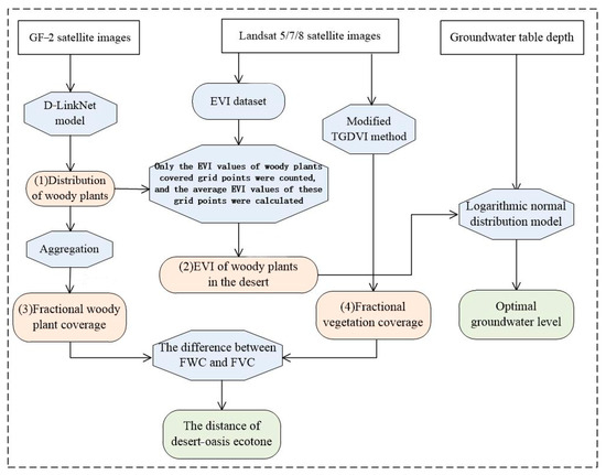
Figure 2.
Technical workflow chart.
Specifically, the map of woody plants with a resolution of 1 m was extracted from GF-2 images, and then it was aggregated to create a coverage map of woody plants with a 30-m resolution to match the resolution of Landsat images. After that, it was overlaid with EVI data derived from Landsat images to obtain EVI values for woody plants within each 30-m resolution grid. This method effectively eliminates interference from background factors such as bare soil, biological soil crusts and herbaceous vegetation. Therefore, it could more accurately reflect the growth trend of woody plants for a long time. For the schematic diagram, see Figure 3.
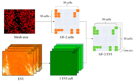
Figure 3.
Schematic diagram for calculating the time-series enhanced vegetation index (EVI) for woody plants combined GF-2 and Landsat satellite images.
2.3.1. Extraction of Woody Plant Distribution
GF-2 images, with their high resolution and rich textural features, provided a significant advantage for extracting detailed features using a neural network model. Preprocessed GF-2 images were cropped to 128 × 128 pixels after selection, and corresponding sample labels were generated through visual interpretation. For small-sample training, sample augmentation was required to enhance model robustness and generalizability. Standard methods of sample augmentation included geometric transformations (rotation and flipping), color transformations, image brightness and contrast transformations, cropping and adding noise. This study applied random cropping, rotation, and flipping to the original samples, increasing each sample 64 times. The final dataset included 1600 nonrepeating sample labels of 128 × 128 pixels, which were divided into training, validation and testing sets at a 6:2:2 ratio.
This paper selected three classical CNN-based semantic segmentation models (D-LinkNet, FCN8S, DeepLab), which were widely used in remote sensing semantic segmentation tasks [20]. Comparison results showed that the D-LinkNet model achieved the highest accuracy and was therefore chosen to extract the distribution of woody plants in this study area. Originally designed for road segmentation tasks [21], the D-LinkNet model employs encoder-decoder architecture, atrous convolutions and a pretrained encoder. Atrous convolutions enable the expansion of the model’s receptive field without reducing the resolution of the feature map.
The accuracy evaluation indicators include the producer’s accuracy (PA), user’s accuracy (UA), overall accuracy (OA), F1-score and mean intersection over union (MIoU). The PA is the proportion of correctly predicted pixels among the pixels in the predicted output. The UA is the proportion of correctly predicted pixels among the true-value pixels in the field survey. The OA is the proportion of correctly predicted pixels among all pixels. The F1-score is another metric used to gauge the performance of a classifier. The MIoU calculates the average ratio of the intersection to the union for all categories. The calculation formulas were as follows:
where TP, TN, FP and FN represent the number of pixels in the true positive class, the true negative class, the false positive class, and the false negative class, respectively.
2.3.2. Enhanced Vegetation Index
The enhanced vegetation index (EVI) has been proven to minimize canopy-soil variations and enhance vegetation signals. Therefore, EVI has been widely used for vegetation monitoring, ecological assessment, and climate change response in arid and semi-arid regions [22]. In this study, EVI was calculated based on Landsat images and the following formula:
where Rnir, Rred and Rblue represent the near-infrared (NIR), red and blue light reflectance values after atmospheric correction for Landsat images, respectively. G is the grain coefficient, L is the soil background adjustment parameter and C1 and C2 are coefficients for correcting the atmospheric influence on the red band via the blue band. Generally, L = 2, C1 = 6, C2 = 7.5 and G = 2.5.
2.3.3. The Modified Three-Band Maximum Gradient Difference (TGDVI) Method
The modified TGDVI method strengthens the spectral difference between sparsely vegetated areas and bare soil. Thus, it is suitable for estimating the fractional vegetation cover (FVC) in sparsely vegetated areas [23]. The formula is expressed as follows:
where FVC represents the fractional vegetation cover in the vegetation-covered area; Rred, Rnir and Rswir represent the red, NIR and shortwave infrared (SWIR) light reflectance values after atmospheric correction; λred, λnir and λswir represent the wavelengths of the red, NIR and SWIR bands, respectively; and dmax represents the d value estimated by the modified TGDVI for the area fully covered by vegetation. Combined with FVC observation data, we determine that the dmax values corresponding to areas with an NDVI ≥ 0.6 represent fully vegetated areas in the temperate deserts of northern Xinjiang.
2.3.4. Method of Calculating the Optimal Groundwater Level
A study in arid regions of Northwest China showed a skewed normal distribution of desert plant growth in relation to the groundwater table [24]. Therefore, this study employed a normal distribution model to establish the relationship between the EVI and GTD of two typical woody plants (H. ammodendron and T. ramosissima) in the lower reaches of SRB. The formula for the model was as follows:
where c represents the EVI, x represents the GTD, μ is the mean value of ln(x), and σ is the tolerance range of plants to the GTD. The formulas for calculating the maximum EVI value corresponding to the GTD (Xmax), the mean value of the GTD (E(x)) and the variances in the GTD (σ(x)) are as follows:
where E(x) represents the mean value of the GTD associated with woody plant growth and σ(x) indicates the tolerance of woody plants to the GTD.
3. Results
3.1. Extraction Results of the Woody Plant Distribution
3.1.1. Results of Accuracy Evaluation
All three models effectively extracted woody plants, and the accuracy assessment results for each model are presented in Table 1:

Table 1.
Comparison of accuracy for the three neural network models.
The comparison showed that the training results of the D-LinkNet model demonstrated good accuracy, with PA, UA and F1-scores all exceeding 0.67 and an OA of up to 96.06%. Considering the fragmentation characteristics of woody plants, there might be some errors near the boundaries in the model recognition results. However, we believe that the recognition results meet the accuracy criteria. Although the OA of the FCN8S and DeepLabV3 Plus models also exceeded 91%, other metrics, such as the F1-score and MIoU, performed poorly.
3.1.2. Results of Woody Plant Extraction
Figure 4 shows the GF-2 satellite images and the extraction results corresponding to the three neural network models. All three models successfully identified the distribution area of woody plants. The DeepLabV3 Plus model demonstrated inferior edge smoothness in its extraction results, with noticeable interconnectivity between patches. Compared to DeepLabV3 Plus, the FCN8S model produced isolated patches of individual woody plants, although these patches were significantly smaller than the actual canopy diameter. Both models exhibited notable under-segmentation, likely due to the loss of local detail during the upsampling process. In contrast, the D-LinkNet model yielded the best performance, achieving a balance between edge smoothness and extraction accuracy, while demonstrating strong robustness and generalization capabilities.
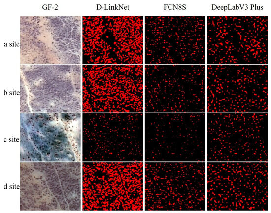
Figure 4.
Detailed comparison of woody plant mapping using three models at four sample sites. (a), (b), (c) and (d) represent the number of each sample site. Red represents extracted patches of woody plants.
3.2. Fractional Woody Plants Cover
The mapping of woody plants extracted by GF-2 images with a spatial resolution of 1 × 1 m was resampled onto the grid with a 30 × 30 m resolution of the corresponding Landsat images. Thus, the fractional woody plant coverage (FWC) with a resolution of 30 m was generated (Figure 5a). Figure 5b shows the FVC extracted by the modified TGDVI method based on Landsat images during the same period.
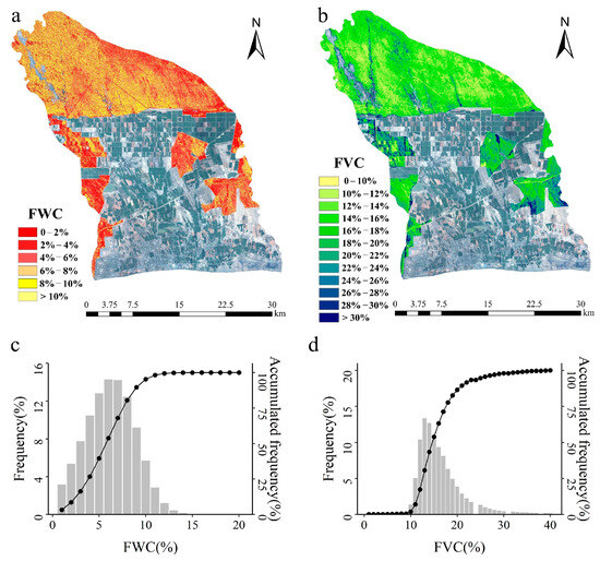
Figure 5.
(a) the maps of fractional woody plant cover (FWC) in the middle and lower reaches of the SRB; (b) the maps of fractional vegetation cover (FVC) in the middle and lower reaches of the SRB; (c) the statistical distribution of FWC (d) the statistical distribution of FVC.
The values of FWC extracted from GF-2 images using a deep learning method were relatively low in desert areas. Approximately 95.33% of the desert regions had an FWC of less than 10%, with more than half the area (53.49%) having an FWC of between 4% and 8% (Figure 5a). In contrast, the FVC extracted from Landsat images using the modified TGDVI method is relatively greater. Approximately 85.02% of the areas had FVC values in the range of 10–20%. Approximately 47.55% of the total area had FVC values ranging from 12% to 16%. The desert zone embedded within the oasis had a 16–20% higher FVC than the northern desert zone due to the positive influence of irrigation water from the surrounding agricultural land. However, most woody plants here were cleared for croplands, resulting in a low FWC (<3%). Lower values of FWC and FVC were located away from the desert-oasis ecotone, while higher values were located within the reach of drainage channels.
In order to quantify the spatial stability of vegetation distribution in the northern desert, 25 buffer zones with 100-m intervals were divided at equal distances from the oasis to the north, and the average FWC and FVC within the buffer zones were calculated (Figure 6a). Moreover, the difference between the FWC and FVC could be roughly considered the coverage of other ephemeral plants in the desert (Figure 6b). In the buffer zone 15 km from the oasis, the average FWC value increased from 4.78% to 6.54%, while the average FVC value decreased from 24.57% to 14.46% (Figure 6a). It indicated that many woody plants were cultivated on cropland near the oasis, resulting in a low FWC. In contrast, deserts far from oases had little land-clearing activity, so FVC remained stable. In the desert closer to the oasis, the FVC of newly reclaimed cropland was generally higher than that of natural vegetation, and irrigation also promoted the growth of herbaceous vegetation around cropland, resulting in higher FVC here. The Mann-Kendall test showed that the FWC was lower and the FVC was significantly greater in the desert area within 1.0 km of the oasis (Figure 6b). In contrast, in the desert area 1.0 km away from the oasis, the difference between the FWC and FVC remained approximately 8% with less human disturbance. Therefore, the desert–oasis ecotone in the lower reaches of the SRB was defined as the area approximately 1.0 km away from the oasis.
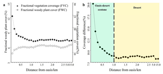
Figure 6.
(a) represents the change curves of FVC and FWC, and (b) represents the differences between FVC and FWC within 15 km from oasis.
3.3. The Spatio-Temporal Variation of EVI in the Middle and Lower Reaches of the SRB
Between 1988 and 2021, most of the vegetation-covered areas in the study area exhibited an increasing trend in the EVI, with only 2.04% of the vegetation-covered areas experiencing a decrease in the EVI. We divided the portions with EVI slopes greater than 0 into six types: I (0–0.94 × 10⁻³), II (9.41 × 10⁻⁴–5.30 × 10⁻³), III (5.30 × 10⁻³–6.68 × 10⁻³), IV (6.68 × 10⁻³–8.06 × 10⁻³), V (8.06 × 10⁻³–12.42 × 10⁻³) and VI (12.42 × 10⁻³–26.21 × 10⁻³) (Figure 7a). Approximately 73.62% of the vegetation-covered areas had EVI slopes of type I and II (Figure 7b). Areas with a rapid increase in EVI were concentrated in the newly created cropland in the eastern APOL, western APOU and eastern ADFO areas, with all of these areas categorized as level VI in terms of EVI change rates. The desert areas exhibited a slow increase in the EVI, with the EVI slope ranging from level I to level II. The average annual slope of the EVI in the desert areas was 9.44 × 10⁻⁴ (p < 0.001, R2 = 0.28), while in the oasis areas, it was 4.78 × 10⁻³ (p < 0.001, R2 = 0.61), which was 5.06 times greater than that in the desert areas (Figure 7c).
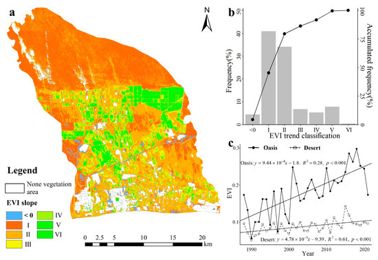
Figure 7.
Spatiotemporal variations (a), statistical distribution (b) and annual time series (c) of the EVI from 1988 to 2021 in the middle and lower reaches of the SRB.
3.4. The Relationship Between EVI and GTD in the Middle and Lower Reaches of the SRB
We selected 22 monitoring wells for each site with EVI within the site’s 100 × 100 m buffer zone. After that, we divided the three ecohydrological zones of the study area into subcategories according to the GTD and proportion of cropland area. The basis for the classification is shown in Table 2.
Table 2.
Classification of the subcategories in the middle and lower reaches of the SRB.
In APOL-1, when GTD ranged from 0.88 to 8.19 m and the proportion of cropland was less than 60%, EVI exhibited a strong quadratic relationship with GTD (p < 0.001, R2 = 0.17) (Figure 8a). EVI values initially increased and then decreased with increasing GTD, reaching a maximum value at a GTD of 5.1 m. In APOL-2, when GTD ranged from 1.97 to 3.42 m and the proportion of cropland was greater than 70%, EVI showed a significant negative linear relationship with GTD (p < 0.001, R2 = 0.25) (Figure 8b). In APOU-1, when GTD ranged from 1.48 to 7.07 m and the proportion of cropland was less than 40%, EVI exhibited a significant quadratic relationship with GTD (p < 0.05, R2 = 0.19) (Figure 8c). Consistent with the pattern of APOL-1, EVI values increased and then decreased with increasing GTD, reaching a peak at a GTD of 4.6 m. In APOU-2, EVI showed a significant logarithmic relationship with GTD (p < 0.001, R2 = 0.24) when GTD ranged from 0.31 to 26.17 m and the percentage of cropland was greater than 85% (Figure 8d). In ADFO-1, when GTD ranged from 62.81 to 73.07 m and the proportion of cropland was less than 45%, EVI exhibited an exponential relationship with GTD (p < 0.001, R2 = 0.26) (Figure 8e). In ADFO-2, when GTD ranged from 0.71 to 37.51 m and the proportion of cropland exceeded 65%, EVI also exhibited an exponential relationship with GTD (p < 0.001, R2 = 0.14) (Figure 8f).
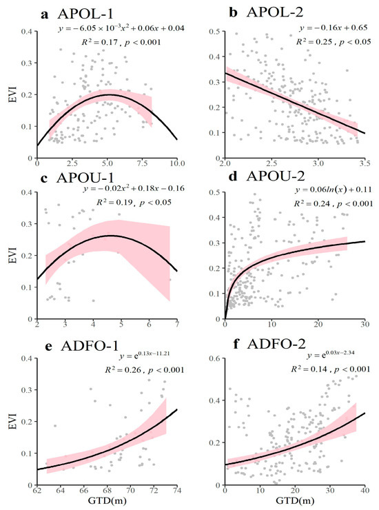
Figure 8.
Impact of GTD on EVI for (a,b) APOL, (c,d) APOU and (e,f) ADFO in the middle and lower reaches of the SRB. The pink-shaded region shows the 95% confidence interval of the regression.
Based on the different water utilization strategies of woody plants, we quantified the relationship of EVI with precipitation and GTD in T. ramosissima and H. ammodendron (Figure 9). In the buffer zone of H. ammodendron site, when GTD ranged from 7.44 to 8.02 m and PRE was less than 75 mm, EVI exhibited a quadratic relationship with GTD (p < 0.001, R2 = 0.24) (Figure 9a). EVI initially decreased and then increased with increasing GTD, and it reached a minimum value when GTD was 7.80 m. Furthermore, EVI also exhibited a positive relationship with PRE (p < 0.001, R2 = 0.14) (Figure 9b). In the buffer zone of T. ramosissima site, when GTD ranged from 1.88 to 7.69 m and PRE was less than 80 mm, EVI exhibited a quadratic relationship with GTD (p < 0.001, R2 = 0.21) (Figure 9c). EVI increased and then decreased with increasing GTD, peaking at a GTD of 6.18 m. However, there was no significant relationship between the PRE and EVI in this site (Figure 9d).
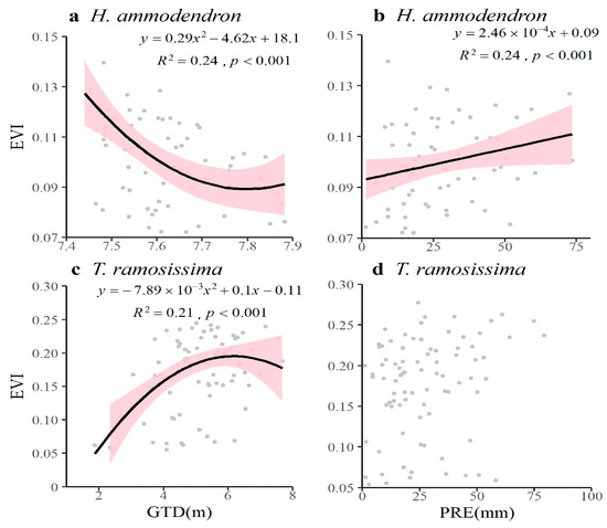
Figure 9.
Impact of GTD and precipitation (PRE) on EVI for (a,b) H. ammodendron and (c,d) T. ramosissima in the lower reaches of the SRB. The pink-shaded region shows the 95% confidence interval of the regression.
3.5. The Optimal GTD Values of Two Woody Plants
In the buffer zone of two woody plant sites, we established a logarithmic normal distribution fitting for the H. ammodendron and T. ramosissima sites using EVI and GTD data (Figure 10).
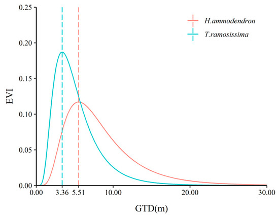
Figure 10.
Diagram of the lognormal distribution fit between EVI and GTD for H. amodendron (red) and T. ramosissima (green) in the lower reaches of the SRB.
The optimum GTD values (also known as the optimum groundwater table) for the H. ammodendron and T. ramosissima sites were calculated to be 5.51 m and 3.36 m, the average GTD values were 8.48 m and 5.26 m, and the GTD variances were 4.89 m and 3.10 m, respectively.
4. Discussion
4.1. The Influences of Climate Change and Human Activities on Woody Plants
Since the 1980s, Xinjiang Province has experienced significant warming and humidification, with increases in both extreme precipitation and extreme drought [25,26]. The combination of a warm, humid climate and intense evaporation has accelerated the local precipitation cycle. Under this warm-wet tendency, vegetation in the Junggar Basin, Tianshan Mountains, Altai Mountains of Northwest Xinjiang is likely to experience a significant greening trend [27]. Meanwhile, cropland expansion and desertification control efforts have been recognized as major anthropogenic factors in the improvement of vegetation [28]. The abrupt increase in cropland area mainly came from the reclamation of land surrounding or downstream of desert woody plants, which intensified agricultural water demand and reduced the ecological water supply in deserts [29]. This led to the over-pumping of rivers and over-exploitation of groundwater, causing rivers to dry up and GTD to decline in arid regions [30]. In additional, the widespread promotion of water-saving technologies (e.g., drip irrigation under film mulch) in arid regions has decreased field infiltration from lining canals future decreasing groundwater recharge [31]. Therefore, it poses a serious threat to the survival of woody plants in desert regions, which depend on shallow or deep soil water and groundwater.
More than half (53%) of the world’s GDEs exist within regions experiencing declining groundwater trends [8]. Based on GRACE data, groundwater storage in Northwest China showed a continuous decreasing trend over the past nearly 40 years, especially in the North Tianshan Rivers Basin (including the Gurbantunggut Desert) [32,33]. The overexploitation of groundwater due to human activities has been an important factor contributing to this decline. In the future, groundwater storage is likely to continue to decline due to rising agricultural irrigation demands in Northwest China [34]. Under future climate scenarios, the potential suitable distribution of plants in cold deserts is expected to increase, assuming no human influence [35]. It implies that, in the future, if the expansion of irrigated agriculture and agricultural water consumption is not scientifically managed, woody plants in arid regions will continue to face the risk of degradation, even under favorable climate change conditions.
4.2. The Responses of Woody Plants to the Decreased GTD
Woody plants in arid regions possess unique ecophysiological characteristics and have developed various drought resistance mechanisms to cope with both hydrological and climatic drought conditions [36,37,38]. As dominant vegetation in GDEs, these plants exhibit a wide range of groundwater use strategies and plasticity. They can adjust their water uptake depth and modify their water-use strategies in response to variations in groundwater depth [39]. Due to different groundwater dependencies, T. ramosissima and H. ammodendron exhibit distinct responses to declining groundwater depth in arid regions. H. ammodendron is a dominant deep-rooted species that primarily utilizes deep soil water and groundwater [40]. In this study, H. ammodendron primarily relies on shallow soil water recharged by plentiful snowmelt water and large precipitation events in the spring (April), while it shifts its water source to deep soil water and groundwater in summer and autumn (June to September). Meanwhile, T. ramosissima lies between deep-rooted and shallow-rooted plants and simultaneously utilizes shallow, middle and deep soil water [38]. When in a region or season with more precipitation, T. ramosissima predominantly relies on shallow soil water. When shallow soil moisture is insufficient, it gradually shifts to using its deeper roots to absorb water from deeper soil layers and groundwater [41].
Flexible water uses strategies in different plants to adapt to climatic or hydrological droughts have also been reported in other arid regions. In the Sahelian, trees restrict their reliance on soil moisture during the dry season, as their roots extend to access the water table [42]. The temporal relationship between NDVI and terrestrial water storage (TWS) was slightly stronger than that between NDVI and rainfall in the semi-arid Sahel [43]. During the dry season, groundwater serves as a significant water source for riparian forests’ transpiration, probably contributing to more than 50% of total transpiration in a tropical savanna riparian zone of Australia [44]. The woody plants in arid grasslands and deserts have been found to extract water from depths up to four times greater than trees in humid temperate forests [45]. It shows that woody plants in arid regions are more dependent on groundwater than forests in humid areas.
4.3. The Optimal GTD of Woody Plants in Northwest China
The optimal GTD for drought adaptation of H. ammodendron and T. ramosissima in inland river basins of Northwest China due to different hydrological conditions in each basin (Table 3). Generally, the optimal GTD for H. ammodendron is less than 5 m [46,47]. However, when the GTD exceeds 10 m, H. ammodendron faces water scarcity, leading to severe degradation [47]. T. ramosissima which is distributed across the Heihe River Basin, Shiyang River Basin, the Taklamakan Desert and the Tarim River Basin, exhibits significant variations of GTD. Its optimal GTD ranges from 3 to 6 m, but it cannot survive when the GTD exceeds 10 m. Our findings align with those of previous studies.
Table 3.
The GTD of H. ammodendron and T. ramosissima in the inland river basin of Northwest China.
4.4. Limitations and Future Work
Challenges remain in ensuring the quality of time series data generated from Gaofen satellite images [52]. In this study, the spatial distribution of woody plants extracted from Gaofen-2 satellite images in 2021 was used to delineate the area of surviving woody plants. However, using the single classification map of forest, shrub or grassland extracted by remote sensing as a mask may increase uncertainty [53]. Before 2000, large areas of woody plants were reclaimed for cropland in desert regions [54]. As a result, using the 2021 woody plant distribution as a mask could lead to an overestimation of vegetation index values in these reclaimed areas. In future research, we plan to extract the spatial distribution of woody plants since the 1990s using high-resolution foreign remote sensing data sources (e.g., SPOT5, IKONOS, Quickbird) to improve the accuracy of the woody plant’s vegetation index.
Due to the discontinuities and uneven distribution of Landsat images, ensuring the quality of time series generation remains challenging [52,55]. There were 2 years of Landsat images missing (1997 and 2016) and 4 years of Landsat images with a single usable image of the growing season (1988, 1992, 1995 and 1997) in this study. These gaps in Landsat coverage, along with fluctuations in seasonal image availability, introduce uncertainty in reconstructing time-series EVI data for woody plants. The fusion of remote sensing image data among different sensors and the time sequence reconstruction of high-density remote sensing data based on machine learning [56] may be considered to improve the spatial-temporal resolution of historical time-series images in the future.
When using Landsat 5/7/8 images to establish time-series EVI data for woody plants, inter-sensor inconsistencies caused by differences in sensor spectral response and residuals in atmospheric correction were inevitable [57]. These inconsistencies could subtly affect the response of vegetation to climate change [58]. The general linear regression transformation was usually used to make the surface reflectance of Landsat 5/7/8 images consistent. The terrain of the SRB is relatively flat, and the growing season is predominantly characterized by sunny and cloudless days, resulting in minimal differences from atmospheric radiation correction. As Landsat 7 images have contained 22% un-scanned gap pixels since 2003, three types of gap-filling methods (e.g., spatial-based, temporal-based and hybrid methods) have been developed. The ‘gapfill’ method in this study interpolated gaps using spatially neighboring scanned pixels. While this method is generally simple and computationally efficient, it may introduce uncertainty when applied to large gaps or heterogeneous landscapes [59]. The SRB is mainly covered by desert vegetation with a relatively uniform landscape, and ‘gapfill’ method was considered suitable for this study.
In addition, due to the limited number of GTD monitoring wells, it was difficult to accurately obtain the spatial-temporal variations of GTD in the SRB. Currently, this study did not quantify the spatial-temporal variations of EVI and GTD. In future research, a numerical groundwater model or downscaled GRACE products will be employed to simulate the spatial-temporal characteristics of GTD. Furthermore, the relationship between GTD and high-precision vegetation index products of woody plants, retrieved from remote sensing, will be extended to the regional scale.
5. Conclusions and Suggestion
Combining GF-2 and Landsat images, this study developed a long-series EVI dataset (1988–2021) based on woody plants mapping, accurately capturing the spatial-temporal variation of desert vegetation. Additionally, it quantitatively analyzed the relationship between EVI and GTD in the middle and lower reaches of the SRB. The key conclusions are as follows:
- (1)
- The D-LinkNet model effectively extracted the distribution of woody plants from GF-2 satellite images with an overall accuracy (OA) of 96.06%. Combining the actual distribution of woody plants and long time-series Landsat images, the vegetation growth in the middle and lower reaches of the SRB exhibited a significant increasing trend from 1988 to 2021. Furthermore, the growth rate in the oasis areas was much greater than that in the desert areas.
- (2)
- The difference between FWC and FVC served as a reliable indicator of the extent of the desert-oasis ecotone. The desert-oasis ecotone in the SRB of this study was within 1 km north of the oasis boundary.
- (3)
- The two desert woody plants exhibited distinct water-use strategies, resulting in different relationships between their growth and GTD and precipitation in the desert regions of the SRB. The optimal GTD for H. ammodendron and T. ramosissima were 5.51 m and 3.36 m, respectively.
In the arid and semi-arid region of Northwest China, we propose estimating the available water for agricultural irrigation based on the optimal ecological water level of woody plants. This approach will help determine the extent of the oasis area and optimize the planting structure accordingly. Simultaneously, it is essential to strictly control groundwater extraction and continue to implement ecological water release to replenish groundwater in the downstream tail area.
Author Contributions
Conceptualization, J.B.; methodology, H.W. and J.L.; software, H.W.; validation, H.W. and J.Z.; investigation, H.W.; resources, J.B. and R.L.; writing—original draft preparation, H.W.; writing—review and editing, J.B. and X.M.; visualization, H.W.; supervision, J.B. and J.L.; funding acquisition, J.B., J.L., R.L. and X.M. All authors have read and agreed to the published version of the manuscript.
Funding
This research was funded by National Natural Science Foundation of China (Grant No. 42071141), Xinjiang “Tianshan Talents” program project (Grant No. 2023TSYCCX0086), Tianshan Talent-Science and Technology Innovation Team (Grant No. 2022TSYCTD0006), Youth Foundation of Xinjiang Natural Science Foundation (Grant No. 2023D01E19), the Key Program of the Natural Science Foundation of Gansu Province, China (Grant No. 25JRRA646) and the Fengyun Application Pioneering Project (FY-APP-2024.0302).
Data Availability Statement
The data presented in this study are available on request from the corresponding author. The data are not publicly available due to their large size. Readers can also contact the corresponding author if they want data.
Acknowledgments
The authors are very grateful to the China Centre for Resources Satellite Data and Application (https://www.cresda.com/), the United States Geological Survey website (https://earthexplorer.usgs.gov), and the China Meteorological Data Service Centre (http://data.cma.cn).
Conflicts of Interest
The authors declare no conflict of interest.
References
- Zhang, Y.; Tariq, A.; Hughes, A.C.; Hong, D.; Wei, F.; Sun, H.; Sardans, J.; Peñuelas, J.; Perry, G.; Qiao, J.; et al. Challenges and Solutions to Biodiversity Conservation in Arid Lands. Sci. Total Environ. 2023, 857, 159695. [Google Scholar] [CrossRef] [PubMed]
- Huang, J.; Li, Y.; Fu, C.; Chen, F.; Fu, Q.; Dai, A.; Shinoda, M.; Ma, Z.; Guo, W.; Li, Z.; et al. Dryland Climate Change: Recent Progress and Challenges: Dryland Climate Change. Rev. Geophys. 2017, 55, 719–778. [Google Scholar] [CrossRef]
- Koppa, A.; Keune, J.; Schumacher, D.L.; Michaelides, K.; Singer, M.; Seneviratne, S.I.; Miralles, D.G. Dryland self-expansion enabled by land-atmosphere feedbacks. Science 2024, 385, 967–972. [Google Scholar] [CrossRef] [PubMed]
- Wang, C.H.; Li, J.M.; Zhang, F.M.; Yang, K. Changes in the moisture contribution over global arid regions. Clim. Dyn. 2023, 61, 543–557. [Google Scholar] [CrossRef]
- Lian, X.; Piao, S.L.; Chen, A.P.; Huntingford, C.; Fu, B.J.; Li, L.Z.X.; Huang, J.P.; Sheffield, J.; Berg, A.M.; Keenan, T.F.; et al. Multifaceted characteristics of dryland aridity changes in a warming world. Nat. Rev. Earth. Environ. 2021, 2, 232–250. [Google Scholar] [CrossRef]
- Luo, W.C.; Zhao, W.Z.; He, Z.B.; Sun, C.P. Spatial characteristics of two dominant shrub populations in the transition zone between oasis and desert in the Heihe River Basin, China. Catena 2018, 170, 356–364. [Google Scholar] [CrossRef]
- Zhang, C.; Lu, D.; Chen, X.; Zhang, Y.; Maisupova, B.; Tao, Y. The spatiotemporal patterns of vegetation coverage and biomass of the temperate deserts in Central Asia and their relationships with climate controls. Remote. Sens. Environ. 2016, 175, 271–281. [Google Scholar] [CrossRef]
- Rohde, M.M.; Albano, C.M.; Huggins, X.; Klausmeyer, K.R.; Morton, C.; Sharman, A.; Zaveri, E.; Saito, L.; Freed, Z.; Howard, J.K.; et al. Groundwater-dependent ecosystem map exposes global dryland protection needs. Nature 2024, 632, 101–107. [Google Scholar] [CrossRef]
- Li, X.; Song, Z.; Hu, Y.; Qiao, J.; Chen, Y.; Wang, S.; Yue, P.; Chen, M.; Ke, Y.; Xu, C.; et al. Drought Intensity and Post-Drought Precipitation Determine Vegetation Recovery in a Desert Steppe in Inner Mongolia, China. Sci. Total Environ. 2024, 906, 167449. [Google Scholar] [CrossRef]
- Li, E.G.; Tong, Y.Q.; Huang, Y.M.; Li, X.Y.; Wang, P.; Chen, H.Y.; Yang, C.Y. Responses of two desert riparian species to fluctuating groundwater depths in hyperarid areas of Northwest China. Ecohydrology. 2019, 12, e2078. [Google Scholar] [CrossRef]
- Wu, X.; Li, Y.; Xu, G.Q. Response of two dominant woody species to groundwater depth at the transition zone between desert and oasis. Ecol. Indic. 2024, 166, 112278. [Google Scholar]
- Sun, Q.; Zhang, P.; Sun, D.; Liu, A.; Dai, J. Desert Vegetation-Habitat Complexes Mapping Using Gaofen-1 WFV (Wide Field of View) Time Series Images in Minqin County, China. Int. J. Appl. Earth. Obs. 2018, 73, 522–534. [Google Scholar] [CrossRef]
- Liu, M.; Fu, B.; Xie, S.; He, H.; Lan, F.; Li, Y.; Lou, P.; Fan, D. Comparison of Multi-Source Satellite Images for Classifying Marsh Vegetation Using DeepLabV3 Plus Deep Learning Algorithm. Ecol. Indic. 2021, 125, 107562. [Google Scholar] [CrossRef]
- Wu, J.; Li, Y.; Zhong, B.; Liu, Q.; Wu, S.; Ji, C.; Zhao, J.; Li, L.; Shi, X.; Yang, A. Integrated Vegetation Cover of Typical Steppe in China Based on Mixed Decomposing Derived from High Resolution Remote Sensing Data. Sci. Total Environ. 2023, 904, 166738. [Google Scholar] [CrossRef]
- Guo, Y.; Li, Z.Y.; Chen, E.X.; Zhang, X.; Zhao, L.; Xu, E.E.; Hou, Y.A.; Liu, L.Z. A deep fusion unet for mapping forests at tree species levels with multi-temporal high spatial resolution satellite imagery. Remote Sens. 2021, 13, 18. [Google Scholar] [CrossRef]
- Chang, Z.; Li, H.; Chen, D.; Liu, Y.; Zou, C.; Chen, J.; Han, W.; Liu, S.; Zhang, N. Crop Type Identification Using High-Resolution Remote Sensing Images Based on an Improved DeepLabV3+ Network. Remote Sens. 2023, 15, 5088. [Google Scholar] [CrossRef]
- Yin, X.W.; Feng, Q.; Li, Y.; Deo, R.C.; Liu, W.; Zhu, M.; Zheng, X.J.; Liu, R. An interplay of Soil Salinization and Groundwater Degradation Threatening Coexistence of Oasis-Desert Ecosystems. Sci. Total Environ. 2022, 806, 150599. [Google Scholar] [CrossRef]
- Zhu, Q.Q.; Li, Z.; Zhang, Y.N.; Guan, Q.F. Building Extraction from High Spatial Resolution Remote Sensing Images via Multiscale-Aware and Segmentation-Prior Conditional Random Fields. Remote Sens. 2020, 12, 3983. [Google Scholar] [CrossRef]
- Liu, H.; Qi, S.; Liu, L.; Li, X. Analysis of Spatial Heterogeneity of Groundwater Depth in the Fukang Oasis of Xinjiang Based on the Geostatistics. Chin. J. Ecol. 2018, 37, 1484–1489. (In Chinese) [Google Scholar]
- Du, B.; Zhao, Z.R.; Hu, X.; Wu, G.H.; Han, L.Z.; Sun, L.L.; Gao, Q. Landslide susceptibility prediction based on image semantic segmentation. Comput Geosci. 2021, 155, 104860. [Google Scholar] [CrossRef]
- Huete, A.; Didan, K.; Miura, T.; Rodriguez, E.P.; Gao, X.; Ferreira, L.G. Overview of the Radiometric and Biophysical Performance of the MODIS Vegetation Indices. Remote. Sens. Environ. 2002, 83, 195–213. [Google Scholar] [CrossRef]
- Jiapaer, G.; Chen, X.; Bao, A.M. A Comparison of Methods for Estimating Fractional Vegetation Cover in Arid Regions. Agric. For. Meteorol. 2021, 151, 1698–1710. [Google Scholar] [CrossRef]
- Zhao, C.Y.; Li, S.B.; Jia, Y.H.; Jiang, Y.C. Dynamic changes of groundwater level and vegetation in water table fluctuant belt in lower reaches of Heihe River: Coupling simulation. Chin. J. Appl. Ecol. 2008, 19, 2687–2692. (In Chinese) [Google Scholar]
- Zhang, H.; Hu, Z.Y.; Zhang, Z.; Li, Y.M.; Song, S.R.; Chen, X. How does vegetation change under the warm-wet tendency across Xinjiang, China? Int. J. Appl. Earth. Obs. 2024, 127, 103664. [Google Scholar] [CrossRef]
- Jiapaer, G.; Liang, S.L.; Yi, Q.; Liu, J. Vegetation dynamics and responses to recent climate change in Xinjiang using leaf area index as an indicator. Ecol. Indic. 2015, 58, 64–76. [Google Scholar]
- Wang, Q.; Zhai, P.M.; Qin, D.H. New Perspectives on ‘Warming-Wetting’ Trend in Xinjiang, China. Adv. Atmos. Sci. 2020, 11, 252–260. [Google Scholar] [CrossRef]
- Yao, J.Q.; Mao, W.Y.; Chen, J.; Dilinuer, T. Recent signal and impact of wet-to-dry climatic shift in Xinjiang, China. J. Geogr. Sci. 2021, 31, 1283–1298. [Google Scholar] [CrossRef]
- He, P.; Sun, Z.; Han, Z.; Dong, Y.; Liu, H.; Meng, X.; Ma, J. Dynamic characteristics and driving factors of vegetation greenness under changing environments in Xinjiang, China. Environ. Sci. Pollut. Res. 2021, 28, 42516–42532. [Google Scholar] [CrossRef]
- Zheng, X.; Zhu, J.J.; Yan, Q.L.; Song, L.N. Effects of land use changes on the groundwater table and the decline of Pinus sylvestris var. mongolica plantations in southern Horqin Sandy Land, Northeast China. Agric. Water Manag. 2012, 109, 94–106. [Google Scholar]
- Wang, Y.; Xiao, D.; Li, Y.; Li, X. Soil Salinity Evolution and Its Relationship with Dynamics of Groundwater in the Oasis of Inland River Basins: Case Study from the Fubei Region of Xinjiang Province, China. Environ. Monit. Assess. 2008, 140, 291–302. [Google Scholar] [CrossRef]
- Zhang, Q.; Luo, G.; Li, L.; Zhang, M.; Lv, N.; Wang, X. An Analysis of Oasis Evolution Based on Land Use and Land Cover Change: A Case Study in the Sangong River Basin on the Northern Slope of the Tianshan Mountains. J. Geogr. Sci. 2017, 27, 223–239. [Google Scholar] [CrossRef]
- Cheng, W.J.; Feng, Q.; Xi, H.Y.; Sindikubwabo, C.; Chen, Y.Q.; Zhao, X.Y. Spatio-temporal dynamics of water storage across Northwest China over the past four decades. J. Hydrol. Reg. Stud. 2023, 49, 101488. [Google Scholar] [CrossRef]
- Duan, L.; Chen, X.; Bu, L.; Chen, C.; Song, S. Temporal and Spatial Variation Analysis of Groundwater Stocks in Xinjiang Based on GRACE Data. Remote Sens. 2024, 16, 813. [Google Scholar] [CrossRef]
- Cheng, W.; Feng, Q.; Xi, H.; Yin, X.; Cheng, L.; Sindikubwabo, C.; Zhang, B.; Chen, Y.; Zhao, X. Modeling and assessing the impacts of climate change on groundwater recharge in endorheic basins of Northwest China. Sci. Total Environ. 2024, 918, 170829. [Google Scholar] [CrossRef]
- Zhang, L.; Liu, H.L.; Zhang, H.X.; Chen, Y.F.; Zhang, L.W.; Kawushaer, K.; Dilxadam, T.; Zhang, Y.M. Potential distribution of three types of ephemeral plants under climate changes. Front. Plant Sci. 2022, 13, 1035684. [Google Scholar]
- Anderegg, L.D.L.; Anderegg, W.R.L.; Berry, J.A. Not all droughts are created equal: Translating meteorological drought into woody plant mortality. Tree Physiol. 2013, 33, 701–712. [Google Scholar] [CrossRef] [PubMed]
- Hirano, Y.; Todo, C.; Yamase, K.; Tanikawa, T.; Dannoura, M.; Ohashi, M.; Doi, R.; Wada, R.; Ikeno, H. 2018. Quantification of the contrasting root systems of Pinus thunbergii in soils with different groundwater levels in a coastal forest in Japan. Plant. Soil. 2018, 426, 327–337. [Google Scholar] [CrossRef]
- Xu, Y.; Zhao, H.; Zhou, B.; Dong, Z.; Li, G.; Li, S. Variations in water use strategies of Tamarix ramosissima at coppice dunes along a precipitation gradient in desert regions of northwest China. Front. Plant Sci. 2024, 15, 1408943. [Google Scholar] [CrossRef]
- Torres-Garcia, M.T.; Salinas-Bonillo, M.J.; Gazquez-Sanchez, F.; Fernandez-Cortes, A.; Querejeta, J.I.; Cabello, J. Squandering water in drylands: The water-use strategy of the phreatophyte Ziziphus lotus in a groundwater-dependent ecosystem. Am. J. Bot. 2021, 108, 236–248. [Google Scholar] [CrossRef]
- Wu, X.; Zheng, X.J.; Yin, X.W.; Yue, Y.M.; Liu, R.; Xu, G.Q.; Li, Y. Seasonal variation in the groundwater dependency of two dominant woody species in a desert region of Central Asia. Plant. Soil. 2019, 444, 39–55. [Google Scholar] [CrossRef]
- Kulmatiski, A.; Adler, P.; Foley, M. Hydrologic niches explain species coexistence and abundance in a shrub-steppe system. J. Ecol. 2020, 108, 998–1008. [Google Scholar] [CrossRef]
- Huber, S.; Fensholt, R.; Rasmussen, K. Water availability as the driver of vegetation dynamics in the African Sahel from 1982 to 2007. Glob. Planet. Change 2011, 76, 186–195. [Google Scholar] [CrossRef]
- Ndehedehe, C.E.; Ferreira, V.G.; Agutu, N.O. Hydrological controls on surface vegetation dynamics over West and Central Africa. Ecol. Indic. 2019, 103, 494–508. [Google Scholar] [CrossRef]
- Lamontagne, S.; Cook, P.G.; O’Grady, A.; Eamus, D. Groundwater use by vegetation in a tropical savanna riparian zone (Daly River, Australia). J. Hydrol. 2005, 310, 280–293. [Google Scholar] [CrossRef]
- Bachofen, C.; Tumber-Dávila, S.J.; Mackay, D.S.; McDowell, N.G.; Carminati, A.; Klein, T.; Stocker, B.D.; Mencuccini, M.; Grossiord, C. Tree water uptake patterns across the globe. New Phytol. 2024, 242, 1891–1910. [Google Scholar] [CrossRef]
- Jin, X.M. Quantitative Relationship between the Desert Vegetation and Groundwater Depth in Ejina Oasis, the Heihe River Basin. Earth Sci. Front. 2010, 17, 181–186. (In Chinese) [Google Scholar]
- Xu, H.; Li, Y. Water use Strategies and Corresponding Leaf Physiological Performance of Three Desert Shrubs. Acta Bot. Boreali-Occident. Sin. 2005, 25, 1309–1316. (In Chinese) [Google Scholar]
- Peng, H.; Fu, B.; Chen, L.; Yang, Z. Study on Features of Vegetation Succession and its Driving Force in Gansu Desert Areas. J. Desert Res. 2004, 24, 628–633. (In Chinese) [Google Scholar]
- Peng, L.; Wan, Y.B.; Li, H.; Du, M.D.; Shi, Q.D. Influence of surface water and groundwater gradient on spatial distribution of typical vegetation in the hinterland of Taklamakan desert. Sci. Total Environ. 2024, 953, 176060. [Google Scholar] [CrossRef]
- Guo, Z.R.; Liu, H.T. Eco-depth of Groundwater Depth for Natural Vegetation in Inland Basin, Northwest China. J. Arid. Land Resour. Environ. 2005, 19, 157–161. (In Chinese) [Google Scholar]
- Li, Z.; Yaning, C.; Weihong, L.; Xin, L. Responses of Tamarix ramosissima ABA Accumulation to Changes in Groundwater Levels and Soil Salinity in the Lower Reaches of Tarim River, China. Acta Ecol. Sinica. 2007, 27, 4247–4251. [Google Scholar] [CrossRef]
- Fu, Y.; Zhu, Z.; Liu, L.; Zhan, W.; He, T.; Shen, H.; Zhao, J.; Liu, Y.; Zhang, H.; Liu, Z.; et al. Remote Sensing Time Series Analysis: A Review of Data and Applications. J. Remote Sens. 2024, 4, 0285. [Google Scholar] [CrossRef]
- Cheng, K.; Yang, H.T.; Guan, H.C.; Ren, Y.; Chen, Y.L.; Chen, M.X.; Yang, Z.K.; Lin, D.Y.; Liu, W.Y.; Xu, J.C.; et al. Unveiling China’s natural and planted forest spatial–temporal dynamics from 1990 to 2020. ISPRS J. Photogramm. Remote Sens. 2024, 209, 37–50. [Google Scholar] [CrossRef]
- Yin, X.; Feng, Q.; Li, Y.L.; Zhu, W.; Zhang, M.; Yang, L.; Zhang, C.; Wu, X.; Zheng, X. Exaerbated drought accelerates catastrophic transitions of groundwater-dependent ecosystems in arid endorheic basins. J. Hydrol. 2022, 613, 128337. [Google Scholar] [CrossRef]
- Crawford, C.J.; Roy, D.P.; Arab, S.; Barnes, C.; Vermote, E.; Hulley, G.; Gerace, A.; Choate, M.; Engebretson, C.; Micijevic, E.; et al. The 50-year Landsat collection 2 archive. Sci. Remote Sens. 2023, 8, 100103. [Google Scholar] [CrossRef]
- Cao, R.; Xu, Z.; Chen, Y.; Chen, J.; Shen, M. Reconstructing High-Spatiotemporal-Resolution (30 m and 8-Days) NDVI Time-Series Data for the Qinghai-Tibetan Plateau from 2000-2020. Remote Sens. 2022, 14, 3648. [Google Scholar] [CrossRef]
- Vermote, E.; Justice, C.; Claverie, M.; Franch, B. Preliminary analysis of the performance of the Landsat 8/OLI land surface reflectance product. Remote Sens. Environ. 2016, 185, 46–56. [Google Scholar] [CrossRef] [PubMed]
- Chen, X.H.; Zhang, H.K.; Liu, J.P. Making Landsat 5, 7 and 8 reflectance consistent using MODIS nadir-BRDF adjusted reflectance as reference. Remote Sens. Environ. 2021, 262, 112517. [Google Scholar]
- Wang, Q.M.; Wang, L.X.; Wei, C.; Jin, Y.M.; Li, Z.B.; Tong, X.H. Filling gaps in Landsat ETM+ SLC-off images with Sentinel-2 MSI images. Int. J. Appl. Earth. Obs. 2021, 101, 102365. [Google Scholar] [CrossRef]
Disclaimer/Publisher’s Note: The statements, opinions and data contained in all publications are solely those of the individual author(s) and contributor(s) and not of MDPI and/or the editor(s). MDPI and/or the editor(s) disclaim responsibility for any injury to people or property resulting from any ideas, methods, instructions or products referred to in the content. |
© 2025 by the authors. Licensee MDPI, Basel, Switzerland. This article is an open access article distributed under the terms and conditions of the Creative Commons Attribution (CC BY) license (https://creativecommons.org/licenses/by/4.0/).