PhenoCam Guidelines for Phenological Measurement and Analysis in an Agricultural Cropping Environment: A Case Study of Soybean

Abstract

A PhenoCam is a near-surface remote sensing system traditionally used for monitoring phenological changes in diverse landscapes. Although initially developed for forest landscapes, these near-surface remote sensing systems are increasingly being adopted in agricultural settings, with deployment expanding from 106 sites in 2020 to 839 sites by February 2025. However, agricultural applications present unique challenges because of rapid crop development and the need for precise phenological monitoring. Despite the increasing number of PhenoCam sites, clear guidelines are missing on (i) the phenological analysis of images, (ii) the selection of a suitable color vegetation index (CVI), and (iii) the extraction of growth stages. This knowledge gap limits the full potential of PhenoCams in agricultural applications. Therefore, a study was conducted in two soybean (Glycine max L.) fields to formulate image analysis guidelines for PhenoCam images. Weekly visual assessments of soybean phenological stages were compared with PhenoCam images. A total of 15 CVIs were tested for their ability to reproduce the seasonal variation from RGB, HSB, and Lab color spaces. The effects of image acquisition time groups (10:00 $\mathrm{h}$–14:00 $\mathrm{h}$) and object position (ROI locations: far, middle, and near) on selected CVIs were statistically analyzed. Excess green minus excess red (EXGR), color index of vegetation (CIVE), green leaf index (GLI), and normalized green red difference index (NGRDI) were selected based on the least deviation from their loess-smoothed phenological curve at each image acquisition time. For the selected four CVIs, the time groups did not have a significant effect on CVI values, while the object position had significant effects at the reproductive phase. Among the selected CVIs, GLI and EXGR exhibited the least deviation within the image acquisition time and object position groups. Overall, we recommend employing a consistent image acquisition time to ensure sufficient light, capture the largest possible image ROI in the middle region of the field, and apply any of the selected CVIs in order of GLI, EXGR, NGRDI, and CIVE. These results provide a standardized methodology and serve as guidelines for PhenoCam image analysis in agricultural cropping environments. These guidelines can be incorporated into the standard protocol of the PhenoCam network.

1. Introduction

A “PhenoCam” is a near-surface remote sensing system for collecting time-lapse images automatically for phenological studies, but the term also refers to a network of sites (e.g., https://phenocam.nau.edu/webcam/, accessed on 8 February 2025) deploying cameras to track phenological change [1,2,3]. PhenoCam networks have evolved significantly over the past two decades. Recent advancements in PhenoCam networks have demonstrated their versatility in monitoring vegetation dynamics across diverse ecosystems, from agricultural landscapes to natural habitats [4,5,6]. As highlighted by Richardson [7], PhenoCam technology has generated over 200 publications, establishing itself as a fundamental tool in understanding ecosystem responses to climate change.

The increasing adoption of PhenoCams for agricultural monitoring has underscored their potential for providing cost-effective, high-temporal resolution data for crop phenology assessment [5,8]. These methodological advancements have enhanced the reliability of PhenoCam-based vegetation monitoring and expanded its applications through improved image processing techniques [9,10] and standardized protocols for data collection [11,12].Our study builds upon this foundation while extending its application to agricultural systems. The phenological growth stages in plants, such as the timing of emergence, peak greenness, flowering, seed production, and senescence, are crucial for making management decisions [13].

The phenological growth stages are typically displayed by changes in the greenness intensity of the canopy. Several studies have correlated the greenness intensity from PhenoCam images to phenological growth stage dates in forest ecosystems and rangelands [14,15,16]. As of May 2020, there were about 106 agricultural test sites with PhenoCams installed [17]; however, as of February 2025, the number of sites had increased to 839 of vegetation type I, 102 of type II, 39 of type III, 173 of agricultural test sites, (https://phenocam.nau.edu/webcam/gallery/, accessed on 8 February 2025), which suggests the growth and research interest in this field. However, it can be observed that agricultural applications have mapped the greenness intensity only to identify the start and end of the season [18,19]. Therefore, this study used PhenoCam images from two soybean (Glycine max L.) cultivation sites to analyze how the greenness intensity was related to various growth stages of field crops within an agricultural cropping environment along with other objectives.

The PhenoCam-based approach could provide an objective method to assess the crop phenological stages compared to the laborious and subjective manual crop scouting approach. Furthermore, it enables continuous assessment with increased image and temporal resolutions, thereby facilitating early detection of crop stresses by capturing subtle differences in canopy color, and storage of images for long-term assessment and analysis [1,2,15]. Insights into the phenological processes obtained through image analyses from PhenoCam systems, combined with the established agronomic practices, are expected to help improve management decisions [3,20].

However, PhenoCam applications in agricultural systems also face data acquisition and processing challenges, such as a lack of guidelines on suitable color vegetation indices (CVIs) to use for comparison, and appropriate image acquisition time and object position from the camera. Recent agricultural applications have shown promise in using PhenoCams for crop phenotyping [5,8], yield estimation [4,5], and stress detection [21,22], yet standardized protocols for agricultural implementations remain limited. Existing information in the PhenoCam network includes camera setup and installation protocols, archived data products, image analysis tools, and modeling packages, but lacks information on the above-mentioned aspects for agricultural systems. Therefore, it is desirable to use PhenoCam images from agricultural cropping environments and assess their suitability for the extraction of phenological growth stages compared to visual assessments to gain insight and develop guidelines for phenological image analysis.

Using the common red, blue, and green (RGB) channel values from images, CVIs are derived by mathematical expressions of pixel values from two or more color channels to describe canopy color [23,24]. PhenoCam networks have only widely used green chromatic coordinates (GCC) and excess green (EXG) CVIs for monitoring canopy greenness. Even though several other CVIs have been developed and used in different agricultural remote sensing applications [25,26], their applicability to phenological cameras has not been systematically evaluated. The selection of suitable CVIs for PhenoCam applications requires considering multiple factors, such as their existing usage in vegetation monitoring, demonstrated performance in agricultural applications, and mathematical combinations across diverse illumination conditions. RGB-based indices are particularly valuable for PhenoCam networks due to their compatibility with standard digital cameras and cost-effectiveness, while more complex indices incorporating multiple color space transformations may offer enhanced sensitivity to vegetation characteristics [3,7,27,28]. This study evaluates a comprehensive set of CVIs that represent both traditional and enhanced approaches to vegetation monitoring.

Image color intensity variation caused by illumination conditions in agricultural fields is the most common issue in phenological monitoring [29], and another source of variation is camera type [30]. Andresen et al. [31] reported that the GCC and EXG index values fluctuated due to changes in scene illuminations caused by weather and solar radiation. As the PhenoCam images are captured in open atmospheric conditions, abrupt fluctuations in the phenological curve are observed from the images. However, the actual phenological variation (curve) is expected to be smooth with only a slight variation as the crop transitions into different growth stages.

In most of the PhenoCam studies, using either an average or 90th percentile color value from a narrow time window around midday (10:00 $\mathrm{h}$–14:00 $\mathrm{h}$) is recommended to minimize fluctuations from different illumination conditions [32,33]. Koebsch et al. [34] used a broader time window (entire day—05:30 $\mathrm{h}$ to 18:30 $\mathrm{h}$) and minimized the GCC fluctuations by a clustering approach, which determined a common GCC value over a 3-day moving window and assigned to the current time. However, these studies did not quantify the noise produced, nor did they evaluate the suitability of other CVIs. Therefore, the other CVIs might produce a smaller deviation than the GCC and EXG with reference to a smoothed trend representing natural variation.

Richardson et al. [35] suggested plant color evaluated from the pixel intensity values inside a region of interest (ROI) might vary as a function of distance (object position) from the PhenoCam, but it has not been quantified, analyzed statistically, or reported. In general, an ROI is identified within the field of view of the PhenoCam image, and the color information from the ROI is extracted for analysis [15]. Traversing through the PhenoCam image pixels from the bottom to top, the image objects translate to moving away from the camera in the field. Positioning the image ROIs from the bottom to the top represents the object’s position from the PhenoCam. In recent years, PhenoCams have been applied in field phenotyping [5], where the color values from 88 experimental plots were employed in the study. However, the study did not account for the selection of ROIs for extracting color values, which may introduce a higher likelihood of error and potentially affect the accuracy of the inferences drawn. Therefore, analyzing the effect of object positions (through ROIs) on CVIs can be used to determine a suitable ROI position for PhenoCam studies. For this study, we hypothesize that (i) a smoother phenological variation (curve) than GCC will result from other CVIs if they are less prone to noise, and (ii) the image acquisition time and the object position (ROI selection or pixel location) will affect the CVIs describing the soybean phenology.

Given this background, this research aimed to determine a set of CVIs that best represents the natural smooth phenological curve and to evaluate the effects of image acquisition time and object position in the camera’s field of view (through ROI) on the selected CVIs. The results from this research can be incorporated into existing protocols for PhenoCam image analysis for a consistent analysis of crops. The recommendations (CVI, time, and ROI) can be applied in future crop-based studies throughout the PhenoCam network. Therefore, the specific objectives for this research were:

• Evaluate the variations in existing RGB-based CVIs and other novel combinations of alternative color space-based CVIs across image acquisition times (10:00 $\mathrm{h}$–14:00 $\mathrm{h}$ at 30 min intervals for ≈140 days; 2018 growing season).
• Determine a set of best CVIs with a lower variation than the GCC curve and validate the CVI curve against the visually assessed soybean phenological stages.
• Assess the effect of image acquisition time on the selected CVIs within the PhenoCam’s field of view.
• Assess the effect of object position on the selected CVIs within the PhenoCam’s field of view.

2. Materials and Methods

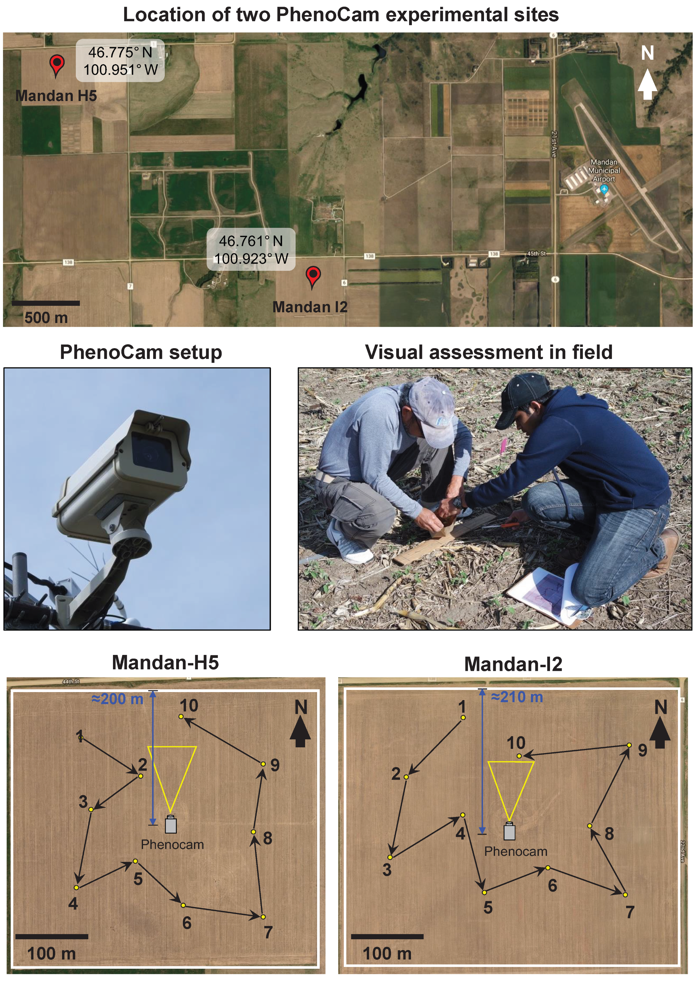
2.1. Site and Management Description

Two experiment fields were selected for the study, namely, Mandan-H5 (46.775°N, 100.951°W) and Mandan-I2 (46.761°N, 100.923°W) at an elevation of 593 $\mathrm{m}$ above sea level, located at the Area 4 Soil Conservation Districts’ Cooperative Research Farm, Mandan, North Dakota, USA (Figure 1). The area of these fields were 19.8 $\mathrm{h}\mathrm{a}$ and 22.1 $\mathrm{h}\mathrm{a}$, respectively. The site has an annual average temperature of 62 °C and receives annual average precipitation of 355–457 mm. During the growing season (April–October), the average temperature is 21–32 °C, with growing season precipitation averaging 190 mm. The soil is predominantly Temvik–Wilton silt loam in both fields. The experimental field had been under a corn–soybean rotation system for the past four years.

Soybean (Mycogen seeds 5B024, The Dow Chemical Company, Midland, MI, USA) was planted using a John Deere 1890 planter at 543,631 seeds/$\mathrm{h}\mathrm{a}$ (220,000 seeds/ac) in both fields on 29 May 2018 and 31 May 2018, respectively. Row and plant spacing were maintained as 0.19 $\mathrm{m}$ and 0.06 $\mathrm{m}$. The soybean crops were harvested on 18 October 2018 and 17 October 2018, respectively.

The dataset employed in this study covered one growing season with a single crop species. It included the PhenoCam imagery with corresponding ground-truth measurements for field validation. Our analysis focused on the geometric relationships between ROI placement and sun position during image acquisition, which are the factors that remain constant irrespective of growing season, climate conditions, or crop type. Therefore, this dataset effectively supported our objective of developing generalizable guidelines for PhenoCam image analysis in agricultural cropping environment.

2.2. PhenoCam Setup and Image Analysis for Crop Phenology

2.2.1. PhenoCam Images and Data File Collection

Both PhenoCam study sites were installed with a NetCam color digital camera (NetCam SC IR, StarDot Technologies, Buena Park, CA, USA). The camera was equipped with a 5-megapixel CMOS sensor. The camera provided a maximum spatial resolution of 2592 × 1944 pixels with frame transfer capability. The sensor featured RGB color channels with 8-bit radiometric resolution per channel (total 24-bit color depth). The camera’s light sensitivity was 0.3 $\mathrm{lx}$ in color mode, and it included automatic exposure control, color balance, and digital noise reduction capabilities for optimal image quality. The digital cameras were housed inside a weather-proof enclosure (Figure 1) for continuous monitoring and were configured based on the instructions provided by the PhenoCam network [36]. The images (30 min interval) were downloaded from the PhenoCam website (https://phenocam.nau.edu/webcam/gallery/, accessed on 8 February 2025) for each field separately (“mandanh5” for the site Mandan-H5 and “mandani2” for site Mandan-I2) by specifying the date range and time span.

The total number of growing days between planting and harvest dates were 143 d for Mandan-H5 and 139 d for Mandan-I2. The images were collected for a time span between 10:00 $\mathrm{h}$ and 14:00 $\mathrm{h}$ on each day as this time span is commonly used in PhenoCam studies [32,33]. The total number of images collected for the entire growing season in Mandan-H5 was 1287 images (143 × 9/d) and 1251 images (139 × 9/d) in Mandan-I2. The details about downloading the images from the PhenoCam network are provided in (Supplementary Materials Section S1; Figures S1–S6).

To assess uncertainties in our data processing and analysis pipeline, we evaluated multiple sources of variation. Image acquisition uncertainty was quantified by analyzing the coefficient of variation for each DAP in color values across different times (10:00 $\mathrm{h}$–14:00 $\mathrm{h}$). ROI selection uncertainty was evaluated by calculating the standard deviation of CVI values across different positions. We evaluated the variability in CVI across different image acquisition times and growth phases.

Along with PhenoCam images, data files (provisional data) that contained several parameters, such as daily mean RGB values, mean GCC, 5–95th percentile RGB values, 3-day mean RGB, etc., also accessible through the PhenoCam website [1,37], were downloaded for analysis. In the present study, the daily mean RGB values from these data files were used to compare different CVIs, as these values were readily available without image processing and represented a broader time span (07:00 $\mathrm{h}$–20:00 $\mathrm{h}$). The procedure for downloading the data files and calculating RGB-based CVIs from the files using an R program [38,39] is presented in (Supplementary Materials Section S2; Figure S7). The images and the data files used in this study belong to the PhenoCam dataset v2.0 [40].

2.2.2. Color Value Extraction from PhenoCam Images

Although a free web-based tool called xROI was available for processing PhenoCam images [41], its capabilities were limited to extracting color values only from RGB color space at a single ROI. But for our study, it was desirable to have a tool that could extract color values from other color space (HSB, Lab) along with RGB at multiple ROIs simultaneously. Therefore, a user-coded plugin was developed using Fiji software (Ver. 1.52p, Rasband [42], Schindelin et al. [43]). The details on the plugin development and its operation can be found in (Supplementary Materials Section S3; Figure S8). The images downloaded from the PhenoCam network resided in a single folder by default. This series of images could be opened by dragging and dropping the entire folder into ImageJ.

The images were opened as a stack, and the user drew a polygonal ROI on any of the images in the stack, which was applied to all the images, to extract color information. The plugin had two inputs (color space and ROI selection) and three color space (RGB, HSB, and Lab) options (Supplementary Materials Figure S8). The user could choose at least one color space and either “Single ROI” or “Multiple ROI” with the number of rows and columns specified. The plugin was developed in such a way that the color values were extracted for all the images in a single run, and the mean RGB, HSB, and Lab values of each sub-ROI (1–9) were generated as a comma-separated value (CSV) file for further analyses.

2.2.3. Color Value Extraction from Multiple ROIs

In this study, multiple ROIs with 3 rows and 3 columns (9 sub-ROIs) were used for color value extraction. Care was taken in specifying the whole ROI so it matched with the ROI specified by the PhenoCam network for Mandan-H5 and Mandan-I2 (Figure 2). To study the effect of time (10:00 $\mathrm{h}$ to 14:00 $\mathrm{h}$ at 30 min intervals) on the CVIs, three replications were considered by averaging the sub-ROIs along each column (replication#: sub-ROIs# ⇒ (1: 1, 4, 7); (2: 2, 5, 8); and (3: 3, 6, 9)).

If the image pixels of a PhenoCam image starting from the bottom to the top were mapped to an actual position in the field, it would correspond to the positions starting from near to far from the camera. Hence, changing the object position can be thought of as selecting the sub-ROI in the vegetation field of view along the image’s vertical direction. A set of three ROIs, which were horizontally at the same level, was assumed to be at the same distances from the vertical plane of the camera. However, as the camera was a point sensor, the horizontal sub-ROIs (as well as the vertical sub-ROIs) had different viewing angles, and this effect of the angle might contribute to the CVIs, which can be a potential parameter to analyze in the future but was not considered in this study. Therefore, to study the effect of object position from the camera on CVIs, the sub-ROIs within each row were considered as replications. The sub-ROIs 1, 2, and 3 served as a replication for testing “far”; similarly, the sub-ROIs 4, 5, and 6 for “middle”; and the sub-ROIs 7, 8, and 9 for “near” (Figure 2). The total distance between the PhenoCam’s position in the field and the field edge in the camera’s direction were ≈200 m and ≈210 m for Mandan H5 and I2, respectively (Figure 1). However, the distance covered in the field by the ROI between the bottom and the top of the whole ROI was ≈120 m, with some margin around the ROI.

2.3. Visual Assessment of Phenological Stages

The visual assessment was performed weekly on each field to record the phenological stages. Additional information on the soybean phenological visual assessment is given in Supplementary Materials Section S4, Figures S9 and S10, and Table S1. Ten random locations were identified in each field and marked with flags for consistently recording phenological stages throughout the growing season (Figure 1; Supplementary Materials Figure S9). At each location, the phenological observation was performed, and five samples were considered as replications (Supplementary Materials Table S1). Soybean phenological stages were identified according to Endres and Kandel [44]. The phenological observation was started after the emergence of seedlings, and all the locations in both fields were assessed on the same day. The vegetative and reproductive stages were indicated with the letters V and R, respectively. The following phenological stages in soybean were considered (Supplementary Materials Figure S10): VC (cotyledon stage), V1 (first trifoliate), V2 (second trifoliate), V3 (third trifoliate), R1 (first flowering), R2 (full bloom), R3 and R4 (pod development), R5 and R6 (seed development), and R7 and R8 (plant maturation). These soybean phenological stages from the visual assessment were distinct and used in the crop phenological assessment, which was then compared to the CVI curves to determine whether any prominent curve features matched with soybean phenological stages.

2.4. CVIs for Phenological Analysis

The selection of the 15 CVIs (12 from RGB space, and 3 from other color spaces) was based on a comprehensive literature review focusing on three key criteria: (i) historical significance in vegetation monitoring—GCC and EXG were included as established benchmarks in PhenoCam networks [18,32]; (ii) proven performance in agricultural applications—NGRDI, GLI, and CIVE were selected based on their successful application in crop monitoring and precision agriculture [25,26]; and (iii) mathematical combinations of different color spaces—CVIs were chosen based on various applications in quantifying vegetation characteristics [27,28,45]. A summary of all the CVIs and their implication is presented in

Table 1. Description and applications of color vegetation indices (CVIs) used in this study.

CVI	Physiological Meaning	References
GCC	Represents the relative proportion of green reflectance in total visible reflectance, directly correlating with chlorophyll content and photosynthetic activity. It is widely used in PhenoCam networks for its simplicity and robustness across illumination conditions.	[18,32]
NGRDI	Normalizes the difference between green and red reflectance, making it sensitive to chlorophyll content and leaf structure changes. It is particularly effective in detecting early-season growth and senescence phases in crops.	[25,26]
NGBDI	Captures the relationship between green pigments and structural components represented by blue reflectance. It is used to distinguish vegetation from soil background, especially in the early growth stages.	[27]
MGRVI	A modified index that uses squared values to enhance sensitivity to green vegetation changes while reducing atmospheric effects. It is more responsive to subtle changes in canopy greenness than simple ratios.	[46]
RGBVI	Combines all three color channels to enhance vegetation detection, particularly effective in discriminating between vegetation and non-vegetation features under varying light conditions.	[47]
NDI	A scaled version of NGRDI that maintains the same physiological sensitivity while providing values in a more intuitive range (0–255), facilitating comparison across different imaging conditions.	[26]
GLI	Emphasizes green vegetation by incorporating all three channels with double weighting for green reflectance. It is effective in detecting subtle changes in canopy greenness during key growth stages.	[48]
RGRI	Simple ratio highlighting the inverse relationship between red and green reflectance, sensitive to chlorophyll degradation during senescence.	[49]
EXG	Emphasizes excess green coloration by double weighting for the green component, making it particularly suitable for detecting healthy vegetation against soil backgrounds.	[50]
CIVE	A linear combination optimized for vegetation extraction, with coefficients derived from a statistical analysis of vegetation spectra. Effective in separating vegetation from the background under various illumination conditions.	[25,51]
VEG	A non-linear index developed to be less sensitive to illumination changes while maintaining sensitivity to vegetation changes. The parameter “a” helps optimize the index for specific vegetation types.	[52]
EXGR	Combines excess green and red information to improve vegetation detection, particularly useful in distinguishing vegetation during different phenological stages.	[26]
${\mathrm{HSB}}_{\mathrm{hue}}$	Represents pure color information independent of brightness and saturation, making it robust against illumination changes. Particularly useful for tracking seasonal color changes.	[53]
${\mathrm{Lab}}_{{\mathrm{a}}^{\prime }}$	Utilizes the green–red opponent color axis from the Lab color space, providing a perceptually uniform measure of vegetation greenness that correlates well with human visual assessment.	[54]
DGCI	Combines hue, saturation, and brightness information to provide a comprehensive measure of “greenness” that correlates well with nitrogen status and overall plant health.	[45]

Note: The expansions and the formulas for calculating these CVIs are given in Section 2.4.1 and Section 2.4.2.

. We excluded indices requiring near-infrared bands or specific calibration procedures, focusing instead on RGB-based indices suitable for standard PhenoCam deployments.

2.4.1. CVIs from RGB Color Space

Twelve CVIs from the RGB color space, which are common in agricultural applications using other imaging platforms (e.g., handheld cameras, unmanned aerial systems) for estimating the vegetation fraction [25], identifying plant biomass [26], and weed monitoring [52], were considered [Equations (1)–(12)].

$$\begin{array}{cc}\hfill \mathrm{GCC}& ={\displaystyle \frac{G}{R+G+B}}\hfill \end{array}$$

(1)

$$\begin{array}{cc}\hfill \mathrm{NGRDI}& ={\displaystyle \frac{G-R}{G+R}}\hfill \end{array}$$

(2)

$$\begin{array}{cc}\hfill \mathrm{NGBDI}& ={\displaystyle \frac{G-B}{G+B}}\hfill \end{array}$$

(3)

$$\begin{array}{cc}\hfill \mathrm{MGRVI}& ={\displaystyle \frac{G^2-R^2}{G^2+R^2}}\hfill \end{array}$$

(4)

$$\begin{array}{cc}\hfill \mathrm{RGBVI}& ={\displaystyle \frac{G^2-B\times R}{G^2+B\times R}}\hfill \end{array}$$

(5)

$$\begin{array}{cc}\hfill \mathrm{NDI}& =128\left({\displaystyle \frac{G-R}{G+R}}+1\right)\hfill \end{array}$$

(6)

$$\begin{array}{cc}\hfill \mathrm{GLI}& ={\displaystyle \frac{2G-R-B}{2G+R+B}}\hfill \end{array}$$

(7)

$$\begin{array}{cc}\hfill \mathrm{RGRI}& ={\displaystyle \frac{R}{G}}\hfill \end{array}$$

(8)

$$\begin{array}{cc}\hfill \mathrm{EXG}& =2g-r-b\hfill \end{array}$$

(9)

$$\begin{array}{cc}\hfill \mathrm{CIVE}& =0.441r-0.881g+0.385b+\mathrm{18.787,45}\hfill \end{array}$$

(10)

$$\begin{array}{cc}\hfill \mathrm{VEG}& ={\displaystyle \frac{g}{r^a{b}^{(1-a)}}}\hfill \end{array}$$

(11)

$$\begin{array}{cc}\hfill \mathrm{EXGR}& =\mathrm{EXG}-1.4r+g\hfill \end{array}$$

(12)

In these equations, GCC is the green chromatic coordinate; R, G, and B are the red, green, and blue color intensity values of image pixels, respectively; NGRDI is the normalized green red difference index; NGBDI is the normalized green blue difference index; MGRVI is the modified green red vegetation index; RGBVI is the red green blue vegetation index; NDI is the normalized difference index; GLI is the green leaf index; RGRI is the red green ratio index; EXG is the excess green; g, r, b are the green/red/blue proportion; CIVE is the color index for vegetation; VEG is the vegitativen; $a=0.667$ is a parameter in VEG [Equation (11)]; and EXGR is the excess green minus excess red.

2.4.2. CVIs from Other Color Spaces

Three CVIs from other color spaces, HSB (hue, saturation, and brightness) and Lab (Lightness, chroma1, chroma2), tested in the study were the HSB’s hue (${\mathrm{HSB}}_{\mathrm{hue}}$), the Lab’s inverted “a” (${\mathrm{Lab}}_{{\mathrm{a}}^{\prime }}$), and the dark green color index (DGCI) derived from HSB. Of the three CVIs, the dark green color index (DGCI) is a common index used in identifying turfgrass quality [55] and nitrogen status in cotton [56]. The expressions for these CVIs are as follows:

$$\begin{array}{cc}\hfill {\mathrm{HSB}}_{\mathrm{hue}}& =H\hfill \end{array}$$

(13)

$$\begin{array}{cc}\hfill {\mathrm{Lab}}_{{\mathrm{a}}^{\prime }}& =1/a\hfill \end{array}$$

(14)

$$\begin{array}{cc}\hfill \mathrm{DGCI}& ={\displaystyle \frac{(H-60)/60)+(1-S)+(1-B^{\prime })}{3}}\hfill \end{array}$$

(15)

where H, S, and $B^{\prime }$ are the hue, saturation, and brightness, respectively, of the HSB color space; and “a” is the chroma1 of the Lab color space.

Typically, the Lab “a” channel produced an inverted phenological trend; therefore, to follow the commonly associated phenological trend, the “a” channel value was inverted (as “$1/a$”) and used for comparison.

2.5. CVIs Analysis and Selection

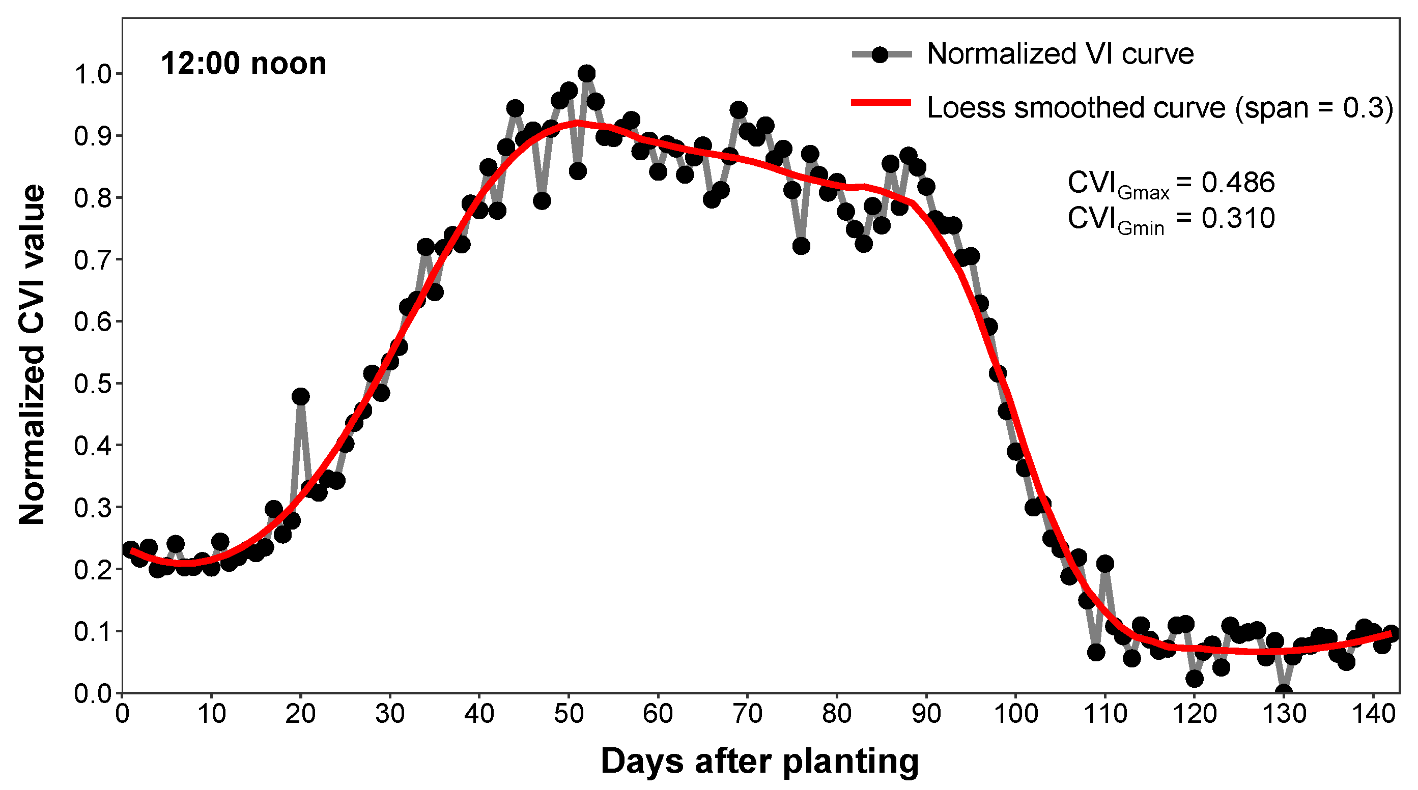
2.5.1. CVI Variation Comparison with Loess Smoothing

To evaluate the variations in a CVI observed trend, it is necessary to have a “reference curve” with which the variation can be compared. A smoothed curve from the respective PhenoCam data served as the reference curve in this study. The smoothed curve corresponding to the selected data was obtained using the loess() function [57], with a span value fixed at 0.3 [32]. This operation determined the smoothed curve parameters, and the R predict() function obtained the values of the smoothed curve.

It can be seen that the observed trend produced from normalized CVI values (raw points) was noisy (Figure 3) when compared to the loess-smoothed curve, and this variation may be due to the temporal variations in CVI values during the measurement period and not because of changes in the plant canopy among subsequent images. These patterns aligned with expected daily changes in solar position and intensity; the specific contribution of illumination conditions could not be quantified as direct light measurements were not collected. While the smoothed curve (red) had a gradual variation and was expected to reflect the actual crop phenological stages.

To determine the undulations in the trend, we used the ribbon or curve length. While other measures are also possible, this comprehensive curve length has physical meaning and is easy to interpret (Supplementary Materials Section S5; Figure S11). With the curve length, an observed trend with greater undulations is longer than a smooth trend [58]. The curve length was calculated as:

$$L_{\mathrm{curve}}=\sum _{i=1}^n\sqrt{1+{({\mathrm{CVI}}_{i+1}-{\mathrm{CVI}}_i)}^2}$$

(16)

where $L_{\mathrm{curve}}$ is the curve length, i is the day after planting, n is the total number of study days, and ${\mathrm{CVI}}_{i+1}$ and ${\mathrm{CVI}}_i$ are the normalized CVI values at a consistent time (e.g., 12:00 $\mathrm{h}$; Figure 4) on the $i+1$ and ith day.

It is practically challenging to minimize variations in the CVI trends caused by natural illumination in open atmospheric conditions. The deviation in length between the normalized raw CVI trend and the reference smooth curve provides a measure of variations caused by scene illuminations and other factors. Therefore, the deviation of the curve length is defined as:

$$L_{\mathrm{dev}}(\%)={\displaystyle \frac{(L_{\mathrm{raw}}-L_{\mathrm{smooth}})}{L_{\mathrm{smooth}}}}\times 100$$

(17)

where $L_{\mathrm{dev}}$ is the deviation of the raw CVI with the smoothed trend (percent), $L_{\mathrm{raw}}$ is the length of the normalized raw CVI trend, and $L_{\mathrm{smooth}}$ is the length of the loess-smoothed curve (pixel). It represents the additional path length a curve takes compared to its smoothed curve. A few advantages of this $L_{\mathrm{dev}}$ are as follows: (i) scale independent—after normalization, $L_{\mathrm{dev}}$ provides a fair comparison between CVIs with different value ranges of other CVIs; (ii) physical interpretability—it directly represents curve roughness as excess path length; and (iii) sensitive to variations—it captures both magnitude and frequency of deviations. We have compared its functionality with the RMSE in (Supplementary Materials Section S5 and Figure S11).

2.5.2. Selection of Best Set of CVIs

The best set of CVIs was categorized as those that had a smooth variation across different times of image capture. In this study, the variation in a phenological curve caused by the illumination changes (time effect) was measured using the developed $L_{\mathrm{dev}}$ [Equation (17)]. This measure provided an idea of the extent of noise produced by each CVI with respect to its smoothed curve and was easy to physically interpret.

The $L_{\mathrm{dev}}$ produced by different CVIs was ranked in ascending order at the specific image acquisition time. The individual ranks at a specific time were summed across the time span (10:00$\mathrm{h}$–14:00$\mathrm{h}$), and a cumulative rank was evaluated. Based on the cumulative rank, a set of best CVIs was selected for further analysis.

2.6. Statistical Analysis and Visualizations

Statistical mean separation was performed using Duncan’s multiple range test using the R package agricolae [59]. A mean comparison among $L_{\mathrm{dev}}$ values from different CVIs obtained from daily mean RGB value was performed to determine the CVIs that produced a similar variation. The daily mean RGB values are easily accessible, and they have been used to derive GCC and employed in various applications [60,61,62]. Therefore, it was desirable to compare among CVIs to determine those that produced a similar variation.

To study the effect of time and position (study variables) on the selected CVI’s pattern, each CVI curve was divided into three major growth phases, vegetative, reproductive, and maturity, and the mean comparison was performed with the normalized CVI values to evaluate the separation of the curves. Dividing into three phases has been previously used in the estimation of biomass and other crop growth parameters [19]. The time span of 10:00 $\mathrm{h}$–14:00 $\mathrm{h}$ at 30 min intervals, which produced nine variations, were grouped into three groups—start (10:00 $\mathrm{h}$–11:00 $\mathrm{h}$), midday (11:30 $\mathrm{h}$–12:30 $\mathrm{h}$), and end (13:00 $\mathrm{h}$–14:00 $\mathrm{h}$)—and mean comparisons among these groups were carried out. Similarly, the effect of position from the camera was statistically analyzed for three levels “far,” “middle,” and “near.” The R package ggplot2 [63] was used to visualize the results.

3. Results and Discussion

3.1. Phenology CVI Curves and Visual Assessment

3.1.1. Comparison of GCC Curve with Visual Assessment

The normalized GCC curve obtained from PhenoCam images of two fields, Mandan-H5 and Mandan-I2, followed a similar pattern (Figure 4). Even though the visual assessment was performed weekly, only the significant phenological stages are presented. In both fields, the GCC started to increase rapidly after the VC stage, which is ideally considered as the start of the growing season [44]. The VC stage in the field was characterized by the expansion of leaves, and this was precisely captured in the GCC trend with an increase in the GCC values. It was expected that the soybean would reach the VC stage within 10–15 days after planting (DAP), and this was consistent with our visual assessment and the GCC curve from PhenoCam images.

As the first vegetative stage (V1) was identified on $\approx 23$ DAP, there was no prominent feature observed in the GCC trend except a consistent inclination in the GCC slope. The other vegetative stages (V2 and V3) were short and passed within a week, which was also not captured prominently in the GCC curve. The GCC values further increased and attained their maximum as the soybeans entered into the reproductive stage (R1). This was the stage when soybean started flowering; however, it happened only in the nodes and could not be seen at the canopy level (above) by the PhenoCam. To capture such subtle phenological stages, a close-up camera setup would be desirable, as employed in the PhenoCam experimental site “willamettepoplar” in Oregon [64].

As the soybeans entered the R2 stage, which was identified as “full bloom,” the GCC curve attained the maximum peak on the 49th and 47th DAP in Mandan-H5 and Mandan-I2, respectively (Figure 4). This was a prominent phenological stage and was also characterized by canopy closure in the PhenoCam images. After R2, the GCC gradually decreased when the soybean “pod set” started. The decrease in GCC coincided with the end of flowering and the beginning of pod development that typically starts from the upper four nodes. Therefore, the canopy greenness declined as indicated by a downward slope after R2.

The gradual decrease continues up to 85– 90 DAP, probably reaching the R6 stage called “full seed set.” After R6, the seeds develop (R7) and turn from green to yellow. This phenomenon was observed by a sudden decrease in the GCC value at $\approx 95$ DAP (Figure 4). At that stage, the crop is safe from major stresses [44]. As the crop matures and enters the R8 stage, it starts to shed leaves and transitions from yellow to brown. This was characterized by a further drop in GCC value to almost the minimum value, which indicated the end of the growing season. The crop is usually left in the field for 10–15 days after R8 to reduce the seed moisture content.

These results indicated that the GCC curve followed the actual soybean phenology as observed visually. With such interpretations, the GCC values can be used to obtain the phenological stages, such as VC, R2, and R8, without visiting the fields. The R6 stage might also be noticed with the start of a sharp decline at 85–90 DAP (Figure 4), which was missed in the visual assessment interval; however, this has to be validated in future studies. This could be a tool for organizations such as the USDA’s National Agricultural Statistics Service and university research stations for preparing weekly crop progress reports during the growing season, which are now reported by manually visiting the fields. In future studies, the PhenoCam images can be potentially used to identify stress that causes discolorations in soybean leaves, such as iron deficiency chlorosis, as it has been proven successful with RGB images in aerial and ground sensing platforms [45,65,66,67].

3.1.2. Phenological Curve Pattern of Other CVIs

Soybean phenological curves for all CVIs showed a clear pattern highlighting different growth stages (Figure 5). Among the CVIs, RGRI and CIVE showed an inverse pattern because of their respective mathematical relationships. In the RGRI calculation [Equation (8)], the G value was considered inversely proportional to RGRI, whereas with CIVE [Equation (10)], it was a linear relationship. The increased weight and the negative sign assigned to g (0.881) produced the inverted pattern. Irrespective of the two different patterns (flipped and non-flipped), the phenological stages from visual assessment matched with the prominent features (e.g., peak or valley) of the CVI curve.

Ideally, the VC stage (Figure 5) is expected at 10–15 DAP in the CVI trend. In some of the CVIs, the VC stage was barely noticeable (e.g., NGBDI, RGRI, ${\mathrm{Lab}}_{{\mathrm{a}}^{\prime }}$), making it difficult to identify the start of the growing season, while others (e.g., GCC, NGRDI, GLI, EXG, CIVE, EXGR, ${\mathrm{HSB}}_{\mathrm{hue}}$) prominently exhibited the VC stage. In previous PhenoCam studies, different threshold values, such as 10%, 25%, and 50% of amplitude, were reported to identify the start of the growing season, which means the DAP at which the CVI value exceeds the threshold was identified as the VC stage [1,13]. In our study, since we normalized the CVI values, the threshold value could be directly seen with the graduations in the y-axis (Figure 5). Threshold values appeared to be specific to the CVI used. Based on the observations, a threshold value of 25% was good for many CVIs (e.g., GCC, RGBVI, EXG, VEG, ${\mathrm{HSB}}_{\mathrm{hue}}$) in representing the VC stage.

The peak bloom was identified in all the CVIs at 45–50 DAP, which matched the visual assessment. In a CVI curve, this was the point when it attained the maximum value except for RGRI and CIVE (minimum value). It was interesting to note that the crop growth was uniform in both fields until that point and displayed a minor separation afterward (Figure 5). This separation might be due to actual growth differences between fields or some of the agronomic factors such as field history, soil fertility, and nutrition.

The phenological transition into the maturity stage was faster in Mandan-I2, which matured faster than Mandan-H5 (Figure 5). This was observed with the separation in the CVI trend $>85$ DAP. However, this phenomenon was observed distinctly only with those CVIs in which the VC stage was not noticeable. Evaluating the precipitation data from both fields revealed that Mandan-H5 received comparatively more precipitation than Mandan-I2. This could be a possible reason for the delayed maturity in Mandan-H5, which caused a separation in the CVI curves. In addition, the inherent field conditions, such as topography and moisture availability, would have also produced some differences in crop growth between fields. Further investigations on the field history and other agronomic factors, such as soil type and quality and crop growth measures (e.g., biomass, leaf area index), may reveal the actual cause of separation at this phenological stage.

The end of the growing season was obvious in all CVI trends. This was characterized by the minimum value for all the CVIs, but the maximum value for RGRI and CIVE. After reaching the maturity stage, the CVIs attained a near-constant value without much variation. Some studies identified the end of the growing season using the same threshold value used to identify the start of season stage [13,68]. Similarly, in this study, the threshold value of 25% was useful in identifying the end of the season with most of the CVIs tested. Although the manual selection of CVIs based on “user judgment” to screen the CVIs that matched the phenological stages is an important criterion, it is a subjective approach. Therefore, the selection of CVIs evaluated based on curve smoothness, which indicates the robustness of the image acquisition time and provides better insight into the nature of CVIs trends, is an objective and repeatable approach.

3.2. Statistical Comparison of $L_{\mathrm{dev}}$ and Selection of the Best CVIs

A statistical comparison of $L_{\mathrm{dev}}$ among various CVIs ($\alpha =0.05$) helped in selecting a set of similar CVIs that produced the lowest $L_{\mathrm{dev}}$. The GLI produced the minimum and DGCI produced the maximum deviations (Supplementary Materials Section S6; Figure S12). For all the CVIs from the RGB color space, Mandan-I2 consistently produced significantly higher $L_{\mathrm{dev}}$ ($\alpha =0.05$) than Mandan-H5; while in HSB and Lab color spaces, Mandan-I2 produced lower deviations. This is an interesting observation and provides an insight that the mathematical relationships with the RGB color space and other color spaces are different. Also, the DGCI produced the minimum deviation between the two fields, but the phenological pattern was not as prominent as some of the CVIs, such as GCC, GLI, RGBVI, and VEG (Figure 5). Therefore, modifying the DGCI equation or deriving a new index similar to DGCI would possibly suit phenological applications, which could be an area for future research.

The selection of the best set of CVIs was based on the robustness of the curve at different times of image capture. The $L_{\mathrm{dev}}$ values of other CVIs between 10:00 $\mathrm{h}$ and 14:00 $\mathrm{h}$ at 30 min intervals are presented in

Table 2. Curve length deviations of 15 other CVIs from their respective loess-smoothed curve from the images captured between 10:00$\mathrm{h}$ and 14:00$\mathrm{h}$ during the 2018 growing season of soybean.

Vegetation Index	Curve Length Deviation from Smoothed Curve, ${\mathit{L}}_{\mathbf{dev}}$ ()									Cumulative Rank	Overall Rank
	10:00$\mathrm{h}$	10:30$\mathrm{h}$	11:00$\mathrm{h}$	11:30$\mathrm{h}$	12:00$\mathrm{h}$	12:30$\mathrm{h}$	13:00$\mathrm{h}$	13:30$\mathrm{h}$	14:00$\mathrm{h}$
Mandan-H5
EXGR	$0.119\pm 0.023$ (2)	$0.149\pm 0.014$ (3)	$0.127\pm 0.018$ (3)	$0.101\pm 0.014$ (1)	$0.124\pm 0.021$ (1)	$0.122\pm 0.014$ (1)	$0.094\pm 0.012$ (1)	$0.100\pm 0.015$ (1)	$0.098\pm 0.015$ (3)	16	1
CIVE	$0.115\pm 0.022$ (1)	$0.144\pm 0.013$ (1)	$0.142\pm 0.016$ (5)	$0.103\pm 0.017$ (4)	$0.132\pm 0.024$ (3)	$0.123\pm 0.019$ (2)	$0.113\pm 0.016$ (5)	$0.126\pm 0.024$ (7)	$0.143\pm 0.020$ (8)	36	2
GLI	$0.119\pm 0.021$ (2)	$0.144\pm 0.013$ (1)	$0.145\pm 0.015$ (6)	$0.102\pm 0.017$ (3)	$0.129\pm 0.023$ (2)	$0.125\pm 0.019$ (3)	$0.113\pm 0.015$ (5)	$0.129\pm 0.023$ (8)	$0.148\pm 0.019$ (9)	39	3
${\mathrm{NGRDI}/\mathrm{NDI} }^{†}$	$0.175\pm 0.025$ (7)	$0.177\pm 0.013$ (7)	$0.130\pm 0.019$ (4)	$0.123\pm 0.012$ (6)	$0.162\pm 0.021$ (8)	$0.172\pm 0.011$ (8)	$0.110\pm 0.009$ (4)	$0.113\pm 0.010$ (4)	$0.104\pm 0.014$ (4)	52	4
RGRI	$0.168\pm 0.027$ (6)	$0.211\pm 0.027$ (13)	$0.159\pm 0.032$ (8)	$0.130\pm 0.022$ (8)	$0.144\pm 0.027$ (6)	$0.166\pm 0.021$ (6)	$0.097\pm 0.015$ (2)	$0.113\pm 0.011$ (4)	$0.094\pm 0.013$ (2)	55	5
${\mathrm{GCC}/\mathrm{EXG} }^{†}$	$0.122\pm 0.022$ (4)	$0.150\pm 0.014$ (4)	$0.151\pm 0.017$ (7)	$0.109\pm 0.019$ (5)	$0.140\pm 0.026$ (5)	$0.132\pm 0.022$ (4)	$0.123\pm 0.017$ (9)	$0.139\pm 0.027$ (9)	$0.160\pm 0.023$ (10)	57	6
NGBDI	$0.189\pm 0.030$ (10)	$0.210\pm 0.033$ (12)	$0.171\pm 0.041$ (10)	$0.132\pm 0.028$ (10)	$0.135\pm 0.032$ (4)	$0.168\pm 0.031$ (7)	$0.098\pm 0.019$ (3)	$0.110\pm 0.015$ (3)	$0.090\pm 0.012$ (1)	60	7
MGRVI	$0.183\pm 0.025$ (9)	$0.172\pm 0.010$ (6)	$0.125\pm 0.016$ (2)	$0.125\pm 0.010$ (7)	$0.172\pm 0.020$ (9)	$0.178\pm 0.010$ (9)	$0.116\pm 0.009$ (7)	$0.117\pm 0.010$ (6)	$0.109\pm 0.015$ (5)	60	7
VEG	$0.140\pm 0.029$ (5)	$0.168\pm 0.020$ (5)	$0.171\pm 0.026$ (10)	$0.131\pm 0.028$ (9)	$0.185\pm 0.040$ (11)	$0.161\pm 0.035$ (5)	$0.165\pm 0.030$ (11)	$0.182\pm 0.047$ (11)	$0.215\pm 0.043$ (11)	78	10
RGBVI	$0.202\pm 0.029$ (11)	$0.186\pm 0.020$ (8)	$0.192\pm 0.026$ (12)	$0.159\pm 0.038$ (12)	$0.208\pm 0.041$ (12)	$0.225\pm 0.048$ (11)	$0.196\pm 0.029$ (12)	$0.229\pm 0.046$ (12)	$0.278\pm 0.042$ (13)	103	12
${\mathrm{HSB}}_{\mathrm{hue}}$	$0.244\pm 0.028$ (12)	$0.196\pm 0.002$ (9)	$0.095\pm 0.006$ (1)	$0.101\pm 0.006$ (1)	$0.172\pm 0.010$ (9)	$0.237\pm 0.014$ (12)	$0.141\pm 0.008$ (10)	$0.107\pm 0.007$ (2)	$0.116\pm 0.010$ (6)	62	9
${\mathrm{Lab}}_{{\mathrm{a}}^{\prime }}$	$0.178\pm 0.006$ (8)	$0.198\pm 0.014$ (10)	$0.165\pm 0.006$ (9)	$0.136\pm 0.009$ (11)	$0.160\pm 0.004$ (7)	$0.179\pm 0.010$ (10)	$0.119\pm 0.007$ (8)	$0.158\pm 0.009$ (10)	$0.138\pm 0.010$ (7)	80	11
DGCI	$0.403\pm 0.009$ (13)	$0.206\pm 0.019$ (11)	$0.199\pm 0.017$ (13)	$0.176\pm 0.015$ (13)	$0.277\pm 0.009$ (13)	$0.342\pm 0.020$ (13)	$0.199\pm 0.012$ (13)	$0.251\pm 0.011$ (13)	$0.219\pm 0.006$ (12)	114	13
Mandan-I2
EXGR	$0.113\pm 0.012$ (1)	$0.146\pm 0.007$ (4)	$0.106\pm 0.003$ (4)	$0.136\pm 0.009$ (2)	$0.116\pm 0.013$ (4)	$0.157\pm 0.006$ (3)	$0.136\pm 0.011$ (4)	$0.132\pm 0.011$ (3)	$0.173\pm 0.010$ (3)	28	2
CIVE	$0.119\pm 0.017$ (4)	$0.134\pm 0.014$ (2)	$0.115\pm 0.007$ (6)	$0.138\pm 0.006$ (4)	$0.143\pm 0.009$ (8)	$0.155\pm 0.015$ (2)	$0.162\pm 0.021$ (7)	$0.136\pm 0.022$ (4)	$0.169\pm 0.017$ (2)	39	3
GLI	$0.114\pm 0.016$ (2)	$0.133\pm 0.013$ (1)	$0.114\pm 0.007$ (5)	$0.136\pm 0.007$ (2)	$0.140\pm 0.008$ (7)	$0.146\pm 0.015$ (1)	$0.157\pm 0.020$ (6)	$0.13\pm 0.02$ (2)	$0.163\pm 0.016$ (1)	27	1
${\mathrm{NGRDI}/\mathrm{NDI} }^{†}$	$0.121\pm 0.010$ (5)	$0.166\pm 0.008$ (6)	$0.104\pm 0.011$ (2)	$0.145\pm 0.015$ (7)	$0.104\pm 0.018$ (3)	$0.172\pm 0.013$ (6)	$0.119\pm 0.010$ (2)	$0.137\pm 0.009$ (5)	$0.192\pm 0.014$ (5)	41	4
RGRI	$0.118\pm 0.012$ (3)	$0.178\pm 0.007$ (8)	$0.128\pm 0.018$ (8)	$0.153\pm 0.021$ (8)	$0.118\pm 0.024$ (5)	$0.176\pm 0.016$ (8)	$0.133\pm 0.017$ (3)	$0.146\pm 0.017$ (8)	$0.194\pm 0.022$ (6)	57	8
${\mathrm{GCC}/\mathrm{EXG} }^{†}$	$0.124\pm 0.019$ (6)	$0.138\pm 0.015$ (3)	$0.121\pm 0.008$ (7)	$0.144\pm 0.007$ (6)	$0.154\pm 0.008$ (9)	$0.160\pm 0.018$ (4)	$0.171\pm 0.023$ (8)	$0.141\pm 0.024$ (7)	$0.173\pm 0.019$ (3)	53	6
NGBDI	$0.133\pm 0.013$ (8)	$0.250\pm 0.008$ (12)	$0.174\pm 0.018$ (11)	$0.193\pm 0.020$ (9)	$0.159\pm 0.023$ (10)	$0.192\pm 0.014$ (10)	$0.149\pm 0.011$ (5)	$0.159\pm 0.012$ (9)	$0.208\pm 0.019$ (8)	82	10
MGRVI	$0.125\pm 0.010$ (7)	$0.158\pm 0.009$ (5)	$0.110\pm 0.010$ (4)	$0.143\pm 0.016$ (5)	$0.102\pm 0.018$ (2)	$0.173\pm 0.014$ (7)	$0.118\pm 0.010$ (1)	$0.138\pm 0.009$ (6)	$0.197\pm 0.014$ (7)	44	5
VEG	$0.180\pm 0.033$ (10)	$0.173\pm 0.028$ (7)	$0.164\pm 0.017$ (10)	$0.198\pm 0.016$ (10)	$0.238\pm 0.013$ (12)	$0.237\pm 0.038$ (11)	$0.258\pm 0.043$ (13)	$0.204\pm 0.049$ (11)	$0.234\pm 0.036$ (11)	95	11
RGBVI	$0.209\pm 0.034$ (11)	$0.236\pm 0.039$ (11)	$0.233\pm 0.015$ (13)	$0.246\pm 0.024$ (13)	$0.296\pm 0.020$ (13)	$0.269\pm 0.042$ (12)	$0.256\pm 0.032$ (12)	$0.224\pm 0.045$ (12)	$0.260\pm 0.049$ (12)	109	12
${\mathrm{HSB}}_{\mathrm{hue}}$	$0.234\pm 0.009$ (12)	$0.180\pm 0.005$ (9)	$0.073\pm 0.005$ (1)	$0.127\pm 0.008$ (1)	$0.072\pm 0.012$ (1)	$0.178\pm 0.014$ (9)	$0.191\pm 0.008$ (9)	$0.116\pm 0.003$ (1)	$0.224\pm 0.012$ (10)	53	6
${\mathrm{Lab}}_{{\mathrm{a}}^{\prime }}$	$0.168\pm 0.012$ (9)	$0.228\pm 0.007$ (10)	$0.141\pm 0.018$ (9)	$0.199\pm 0.021$ (11)	$0.139\pm 0.024$ (7)	$0.166\pm 0.018$ (5)	$0.193\pm 0.012$ (10)	$0.164\pm 0.017$ (10)	$0.216\pm 0.022$ (9)	80	9
DGCI	$0.239\pm 0.011$ (13)	$0.272\pm 0.034$ (13)	$0.174\pm 0.032$ (11)	$0.245\pm 0.032$ (12)	$0.217\pm 0.030$ (11)	$0.307\pm 0.036$ (13)	$0.222\pm 0.021$ (11)	$0.282\pm 0.024$ (13)	$0.412\pm 0.025$ (13)	110	13

Note: Values in parentheses indicate rank in ascending order of $L_{\mathrm{dev}}$ among CVIs at a specific time. ^† indicates both CVIs produced the same $L_{\mathrm{dev}}$ with the normalized CVI values (Supplementary Materials Section S5; Figure S11); hence, either of them can be used. EXGR—excess green minus excess red, CIVE—color index of vegetation, GLI—green leaf index, NGRDI—normalized green red difference index, NDI— normalized difference index, RGRI—red green ratio index, GCC—green chromatic coordinate, EXG—excess green, NGBDI—normalized green blue difference index, MGRVI—modified green red vegetation index, VEG—vegitativen, RGBVI—red green blue vegetation index, HSBhue—hue channel value from HSB color space, ${\mathrm{Lab}}_{{\mathrm{a}}^{\prime }}$—inverted “a” channel value from Lab color space, and DGCI—dark green color index. Equations (1) and (15) define the CVIs used.

. Among the CVIs, (i) GCC and EXG, and (ii) NGRDI and NDI, produced the same $L_{\mathrm{dev}}$. This was because these two sets produced the same phenological pattern but on a different scale due to the similarity of the CVI expressions [Equations (1) and (9) and Equations (2) and (6)]. The normalized CVI curves were completely overlapping with each other as demonstrated with an example of GCC and EXG in (Supplementary Materials Figure S11). Therefore, for phenological comparisons, any one of the CVIs can be used (GCC/EXG and NGRDI/NDI).

The $L_{\mathrm{dev}}$ values for both fields ranged between 0.072% and 0.412%, indicating a wide span of noise (Table 1). Some of the CVIs were sensitive to illumination changes and produced high $L_{\mathrm{dev}}$ with low ranks. The CVIs from RGB produced lesser $L_{\mathrm{dev}}$ values and ranked higher than the CVIs from other color spaces. Out of all the CVIs, the EXGR produced the minimum $L_{\mathrm{dev}}$, and DGCI produced the maximum $L_{\mathrm{dev}}$.

Among the CVIs from other color spaces (HSB and Lab), ${\mathrm{HSB}}_{\mathrm{hue}}$ ranked the best, followed by ${\mathrm{Lab}}_{{\mathrm{a}}^{\prime }}$ and DGCI (Table 2). The reason for the low ranking (high $L_{\mathrm{dev}}$) of DGCI was because the S and ${\mathrm{B}}^{\prime }$ channels were influenced by color intensity variation [Equation (15)]. The DGCI was primarily developed for quantifying fine variations in green color in turfgrass [55]; hence, any small change in the intensity value produced more fluctuation, indicating sensitivity to illumination. When only ${\mathrm{HSB}}_{\mathrm{hue}}$ [Equation (13)] was considered, ignoring S and $B^{\prime }$ channels, the $L_{\mathrm{dev}}$ was smaller compared to the DGCI (Table 1).

Based on the overall rank, the best four CVIs selected in the order of high to low ranking were EXGR, CIVE, GLI, and NGRDI/NDI. The $L_{\mathrm{dev}}$ from the daily mean RGB values of three of the selected CVIs, namely, EXGR, CIVE, and GLI, were statistically similar to those of GCC/EXG for both fields, while NGRDI/NDI was significantly different from GCC/EXG (Supplementary Materials S12). The $L_{\mathrm{dev}}$ produced by NGRDI/NDI was the highest among the selected CVIs, and this was evident from the cumulative rank as well (Table 2).

Overall, both fields produced similar ranks for the selected CVIs but in a different order based on $L_{\mathrm{dev}}$ values (Table 1). This difference may be due to the distance between the two fields ($\approx 3.2$ km apart) and possibly due to the difference in the cloud cover during image capture. Even though CIVE exhibited an inverted curve (Figure 5), it produced a low $L_{\mathrm{dev}}$ value among the tested CVIs and across different image acquisition times. This can also be corroborated by a previous study that reported CIVE was minimally affected by illumination conditions [69]. It is interesting to note that these CVIs produced lesser $L_{\mathrm{dev}}$ values and ranked higher than the commonly used GCC/EXG. These results support the hypothesis that some CVIs produce smaller variations than the existing CVIs in describing the soybean phenological stages.

Apart from the aforementioned CVIs, the GCC/EXG was also selected for further analysis and comparison as it has been widely used for phenological studies in the PhenoCam network [31,53]. The selected best four CVIs could be possibly considered in future PhenoCam related measurement and analysis. It will be also worthwhile to validate these CVIs with different crops and ecosystems (forest, rangeland, and agricultural).

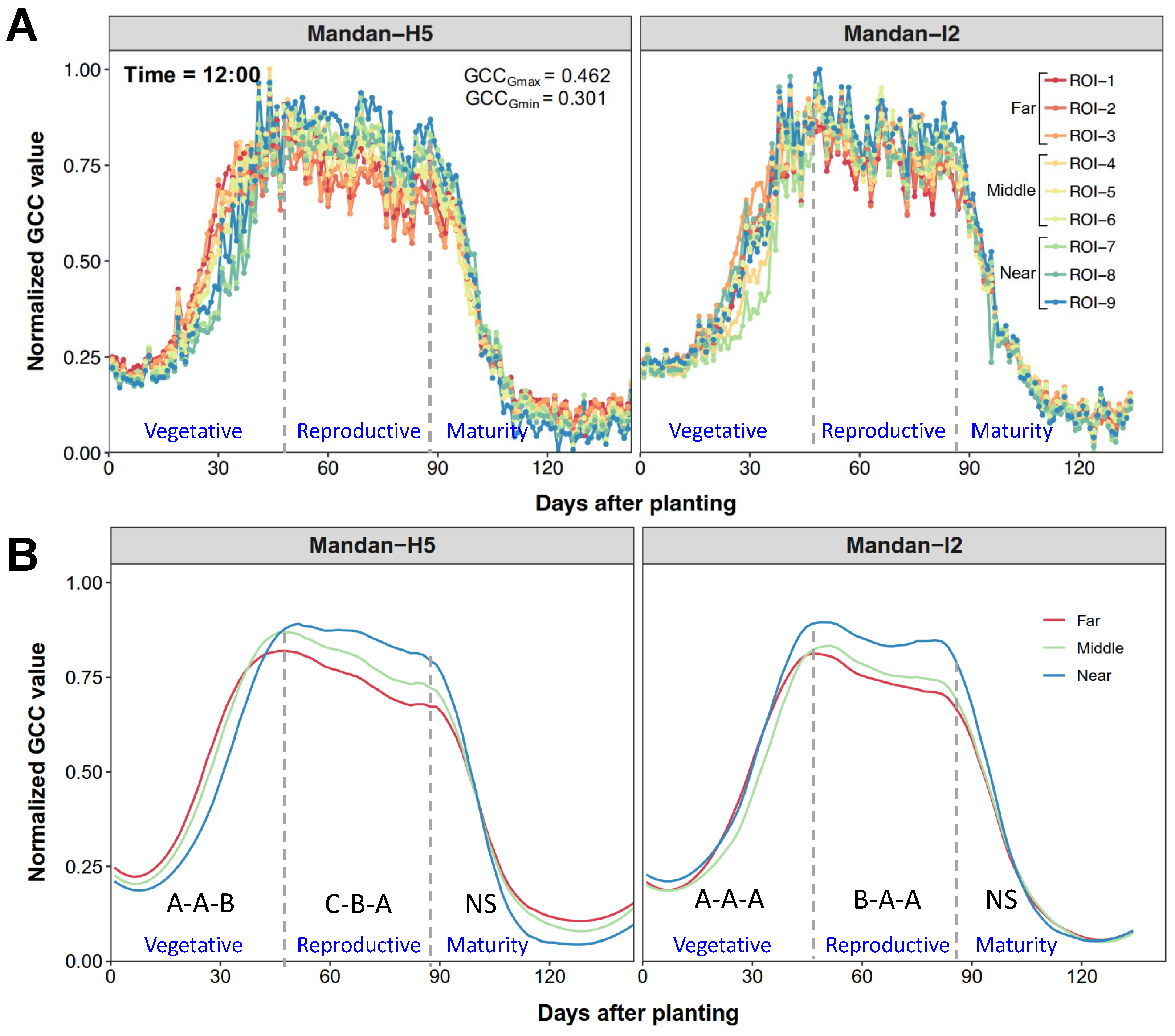
3.3. Effect of Variables and Comparison of Selected CVIs

3.3.1. Effect of Image Acquisition Time on Selected CVIs

The GCC curves at different image acquisition times (10:00 $\mathrm{h}$–14:00 $\mathrm{h}$; nine trends) for the whole ROI are illustrated as an example (Figure 6). Irrespective of the image acquisition time, all GCC curves followed a similar trend (Figure 6A) but produced random fluctuations. The loess-smoothed curves (span = 0.3) of the three time groups (start: 10:00 $\mathrm{h}$–11:00 $\mathrm{h}$, midday: 11:30 $\mathrm{h}$–12:30 $\mathrm{h}$, and end: 13:00 $\mathrm{h}$–14.00 $\mathrm{h}$) are illustrated to demonstrate the separation among curves (Figure 6B). The time groups showed no separation throughout the growing season; however, the observed small separation occurred only during the reproductive phase. This phase is when many phenological changes occur in quick succession, influencing overall color (e.g., flowering, pod set, leaf yellowing).

In the normalized GCC curve with raw data (Figure 6A), all the curves were overlapping and steadily increased until 45– 50 DAP (vegetative phase), beyond which more noise was observed until 40– 85 DAP (reproductive phase). After 85 DAP (maturity phase), all the trends merged again and produced less variation among DAP. The variations among DAP were random and entirely due to ambient conditions. Ideally, the trends are expected to be smooth, but the fluctuations caused by image color differences due to cloud interference with the incoming sun’s radiation are unavoidable. If desired, a color calibration procedure with a color calibration chart should be employed on captured images to minimize these variations [70].

Our uncertainty analysis revealed that temporal uncertainty was minimal during midday hours (11:30 $\mathrm{h}$–12:30 $\mathrm{h}$), with a coefficient of variation typically less than 9.6% for normalized GCC. However, the coefficient of variation during the start (10:00 $\mathrm{h}$–11:00 $\mathrm{h}$) was 11.6%, and it was 11.3% during the end hours (12:00 $\mathrm{h}$–14:00 $\mathrm{h}$). Spatial uncertainty varied by growth phase, with 6.3% during the vegetative phase as the canopy was developing, 5.2% during the reproductive phase as the canopy was fully grown, and 13.9% during the maturity phase as the leaves began to turn yellow and shed. The consistency of CVI calculations across both fields, combined with consistent image acquisition time and growth stages, supports the reliability of our methodology in minimizing measurement variability.

A statistical mean comparison analysis among image acquisition time groups (start, midday, and end) for the selected CVIs at each growth phase is presented in

Table 3. Effect of image acquisition time and object position on selected CVIs within three growing phases and results of statistical comparisons.

		Image Acquisition Time			Object Position
Vegetation Index	Growth Phases	Start	Midday	End	Far	Middle	Near
		(10:00$\mathrm{h}$–11:00$\mathrm{h}$)	(11:30$\mathrm{h}$–12:30$\mathrm{h}$)	(13:00$\mathrm{h}$–14:00$\mathrm{h}$)	(ROI-1–ROI-3)	(ROI-4–ROI-6)	(ROI-7–ROI-9)
Mandan-H5
EXGR	Vegetative	$0.575\pm 0.228$ a	$0.574\pm 0.241$ a	$0.564\pm 0.263$ a	$0.565\pm 0.191$ A	$0.582\pm 0.195$ A	$0.544\pm 0.188$ B
	Reproductive	$0.887\pm 0.055$ a	$0.887\pm 0.061$ a	$0.898\pm 0.060$ a	$0.725\pm 0.085$ C	$0.789\pm 0.074$ B	$0.836\pm 0.054$ A
	Maturity	$0.390\pm 0.164$ a	$0.383\pm 0.161$ a	$0.374\pm 0.154$ a	$0.383\pm 0.139$ C	$0.427\pm 0.141$ B	$0.526\pm 0.139$ A
	Overall	$0.605\pm 0.264$ a	$0.602\pm 0.269$ a	$0.599\pm 0.281$ a	$0.549\pm 0.202$ C	$0.591\pm 0.208$ B	$0.631\pm 0.197$ A
CIVE	Vegetative	$0.494\pm 0.222$ a	$0.486\pm 0.224$ a	$0.486\pm 0.223$ a	$0.387\pm 0.176$ C	$0.428\pm 0.180$ B	$0.482\pm 0.152$ A
	Reproductive	$0.117\pm 0.059$ a	$0.109\pm 0.061$ a	$0.117\pm 0.059$ a	$0.146\pm 0.055$ A	$0.129\pm 0.053$ B	$0.142\pm 0.053$ A
	Maturity	$0.761\pm 0.258$ a	$0.759\pm 0.258$ a	$0.766\pm 0.245$ a	$0.590\pm 0.175$ C	$0.640\pm 0.195$ B	$0.685\pm 0.228$ A
	Overall	$0.474\pm 0.335$ a	$0.469\pm 0.337$ a	$0.474\pm 0.333$ a	$0.384\pm 0.236$ B	$0.410\pm 0.265$ B	$0.448\pm 0.280$ A
GLI	Vegetative	$0.459\pm 0.254$ a	$0.467\pm 0.260$ a	$0.469\pm 0.268$ a	$0.477\pm 0.221$ A	$0.457\pm 0.234$ A	$0.396\pm 0.208$ B
	Reproductive	$0.862\pm 0.057$ a	$0.871\pm 0.060$ a	$0.874\pm 0.057$ a	$0.737\pm 0.071$ C	$0.799\pm 0.063$ B	$0.830\pm 0.056$ A
	Maturity	$0.205\pm 0.240$ a	$0.206\pm 0.239$ a	$0.198\pm 0.232$ a	$0.24\pm 0.175$ A	$0.224\pm 0.193$ A	$0.232\pm 0.227$ A
	Overall	$0.492\pm 0.342$ a	$0.497\pm 0.345$ a	$0.496\pm 0.349$ a	$0.473\pm 0.266$ A	$0.481\pm 0.299$ A	$0.474\pm 0.312$ A
${\mathrm{NGRDI}/\mathrm{NDI} }^{†}$	Vegetative	$0.577\pm 0.188$ a	$0.581\pm 0.198$ a	$0.572\pm 0.194$ a	$0.593\pm 0.183$ A	$0.547\pm 0.187$ B	$0.498\pm 0.160$ C
	Reproductive	$0.906\pm 0.063$ a	$0.902\pm 0.066$ a	$0.893\pm 0.066$ a	$0.841\pm 0.066$ B	$0.831\pm 0.067$ A	$0.812\pm 0.059$ A
	Maturity	$0.286\pm 0.202$ a	$0.280\pm 0.201$ a	$0.268\pm 0.191$ a	$0.336\pm 0.159$ B	$0.270\pm 0.174$ B	$0.250\pm 0.202$ A
	Overall	$0.573\pm 0.305$ a	$0.570\pm 0.308$ a	$0.560\pm 0.306$ a	$0.578\pm 0.255$ B	$0.556\pm 0.279$ B	$0.607\pm 0.280$ A
${\mathrm{GCC}/\mathrm{EXG} }^{†}$	Vegetative	$0.441\pm 0.255$ a	$0.449\pm 0.262$ a	$0.452\pm 0.270$ a	$0.453\pm 0.222$ A	$0.434\pm 0.235$ A	$0.373\pm 0.208$ B
	Reproductive	$0.851\pm 0.061$ a	$0.860\pm 0.064$ a	$0.863\pm 0.062$ a	$0.714\pm 0.075$ C	$0.780\pm 0.067$ B	$0.813\pm 0.061$ A
	Maturity	$0.195\pm 0.233$ a	$0.196\pm 0.233$ a	$0.188\pm 0.226$ a	$0.222\pm 0.168$ A	$0.208\pm 0.186$ A	$0.217\pm 0.220$ A
	Overall	$0.479\pm 0.34$ a	$0.484\pm 0.344$ a	$0.484\pm 0.348$ a	$0.452\pm 0.263$ A	$0.462\pm 0.297$ A	$0.456\pm 0.311$ A
Mandan-I2
EXGR	Vegetative	$0.443\pm 0.281$ a	$0.438\pm 0.281$ a	$0.448\pm 0.310$ a	$0.498\pm 0.239$ A	$0.504\pm 0.228$ A	$0.478\pm 0.239$ B
	Reproductive	$0.797\pm 0.064$ a	$0.788\pm 0.087$ a	$0.796\pm 0.091$ a	$0.754\pm 0.092$ B	$0.757\pm 0.088$ B	$0.789\pm 0.086$ A
	Maturity	$0.307\pm 0.105$ a	$0.303\pm 0.107$ a	$0.312\pm 0.122$ a	$0.362\pm 0.142$ C	$0.406\pm 0.131$ B	$0.471\pm 0.133$ A
	Overall	$0.516\pm 0.272$ a	$0.510\pm 0.273$ a	$0.518\pm 0.284$ a	$0.536\pm 0.237$ B	$0.545\pm 0.227$ B	$0.591\pm 0.215$ A
CIVE	Vegetative	$0.443\pm 0.197$ a	$0.436\pm 0.201$ a	$0.438\pm 0.203$ a	$0.378\pm 0.157$ B	$0.399\pm 0.150$ AB	$0.421\pm 0.152$ A
	Reproductive	$0.112\pm 0.038$ a	$0.116\pm 0.051$ a	$0.120\pm 0.051$ a	$0.150\pm 0.048$ A	$0.133\pm 0.052$ B	$0.153\pm 0.051$ A
	Maturity	$0.763\pm 0.203$ a	$0.773\pm 0.195$ a	$0.768\pm 0.194$ a	$0.626\pm 0.146$ B	$0.654\pm 0.150$ AB	$0.687\pm 0.169$ A
	Overall	$0.439\pm 0.313$ a	$0.442\pm 0.315$ a	$0.442\pm 0.312$ a	$0.381\pm 0.233$ B	$0.391\pm 0.248$ B	$0.413\pm 0.260$ A
GLI	Vegetative	$0.459\pm 0.248$ a	$0.463\pm 0.251$ a	$0.469\pm 0.261$ a	$0.478\pm 0.222$ A	$0.455\pm 0.219$ A	$0.447\pm 0.219$ A
	Reproductive	$0.846\pm 0.043$ a	$0.842\pm 0.060$ a	$0.844\pm 0.064$ a	$0.790\pm 0.071$ B	$0.815\pm 0.070$ A	$0.829\pm 0.070$ A
	Maturity	$0.189\pm 0.175$ a	$0.172\pm 0.165$ a	$0.183\pm 0.171$ a	$0.223\pm 0.150$ A	$0.217\pm 0.153$ A	$0.213\pm 0.162$ A
	Overall	$0.495\pm 0.327$ a	$0.493\pm 0.328$ a	$0.498\pm 0.330$ a	$0.502\pm 0.283$ A	$0.501\pm 0.293$ A	$0.501\pm 0.302$ A
${\mathrm{NGRDI}/\mathrm{NDI} }^{†}$	Vegetative	$0.593\pm 0.184$ a	$0.595\pm 0.188$ a	$0.588\pm 0.195$ a	$0.645\pm 0.167$ A	$0.623\pm 0.158$ A	$0.617\pm 0.154$ A
	Reproductive	$0.854\pm 0.060$ a	$0.844\pm 0.077$ a	$0.838\pm 0.074$ a	$0.869\pm 0.064$ A	$0.851\pm 0.070$ B	$0.839\pm 0.068$ B
	Maturity	$0.205\pm 0.169$ a	$0.195\pm 0.157$ a	$0.202\pm 0.156$ a	$0.320\pm 0.131$ A	$0.292\pm 0.136$ AB	$0.278\pm 0.152$ B
	Overall	$0.551\pm 0.305$ a	$0.545\pm 0.306$ a	$0.543\pm 0.302$ a	$0.582\pm 0.266$ B	$0.593\pm 0.263$ B	$0.616\pm 0.260$ A
${\mathrm{GCC}/\mathrm{EXG} }^{†}$	Vegetative	$0.438\pm 0.249$ a	$0.443\pm 0.252$ a	$0.449\pm 0.263$ a	$0.453\pm 0.224$ A	$0.431\pm 0.220$ A	$0.422\pm 0.221$ A
	Reproductive	$0.831\pm 0.046$ a	$0.827\pm 0.065$ a	$0.829\pm 0.068$ a	$0.769\pm 0.075$ B	$0.795\pm 0.075$ A	$0.811\pm 0.076$ A
	Maturity	$0.167\pm 0.177$ a	$0.160\pm 0.167$ a	$0.167\pm 0.172$ a	$0.205\pm 0.143$ A	$0.199\pm 0.143$ A	$0.195\pm 0.154$ A
	Overall	$0.478\pm 0.326$ a	$0.476\pm 0.327$ a	$0.482\pm 0.329$ a	$0.481\pm 0.282$ A	$0.480\pm 0.293$ A	$0.481\pm 0.302$ A

Note: ^†—Both CVIs produced the same mean and standard deviation values after normalization, therefore either of them can be used. EXGR—excess green minus excess red [Equation (12)], CIVE—color index of vegetation [Equation (10)], GLI—green leaf index [Equation (7)], NGRDI—normalized green red difference index [Equation (2)], NDI—normalized difference index [Equation (6)], GCC—green chromatic coordinate [Equation (1)], and EXG—excess green [Equation (9)]. Dissimilar letter groups denote significant differences (α = 0.05) in the CVI values among the image acquisition time groups (a) and object position groups (A–C).

. The statistical analysis also revealed that the time groups did not have significant differences ($\alpha =0.05$) in the CVI values for all three phases. The mean values at the reproductive phase were higher for all the CVIs except CIVE because of the inverted curve. The standard deviation (SD) values at the reproductive phase were less, as the distribution of CVI values was in a narrow range. More color changes occurred in the vegetative and maturity phases. The normalized CVI values among the selected CVIs for the overall CVI curve were significantly different within each time group (Supplementary Materials Section S7; Figure S13). Therefore, any time group can be used for comparing CVI curves with phenological stages. This result implies fewer images are required per day to build the phenological trend for a simple analysis, as any consistent time in the range from 10:00 $\mathrm{h}$ to 14:00 $\mathrm{h}$ can be suitable to capture the phenological stages.

3.3.2. Effect of Object Position on Selected CVIs

The daily GCC during the growing season for each sub-ROI of the images, representing the object position, captured at 12:00 $\mathrm{h}$ for Mandan-H5 and Mandan-I2 are presented in Figure 7. In the vegetative phase (up to 45– 50 DAP; Figure 7), the far region (sub-ROIs: 1–3) exhibited higher GCC values than the near region (sub-ROIs: 7–9). The GCC values from the middle region (sub-ROIs: 4–6) were between the observed far and near regions. The loess-smoothed curves are presented (Figure 7B) to observe the separation of the phenological curves from far, middle, and near positions. Even though the crop growth was uniform over the field, this phenomenon was observed because of the plants’ position with respect to the PhenoCam and its oblique viewing angle.

In the vegetative phase, the far region appeared greener than the near region. Since the canopy was not closed, some portions of soil and residue were captured in the near region until 50 DAP. Hence, the GCC values were lower than in the far region, which actually represented a larger area than the area represented by the near ROI. The increased plant density (plants per ROI) in the far ROI presented a greener color even though the field plant density was uniform. Furthermore, the far region appeared blurry, due to the image depth and viewing angle, which eliminated the details of soil and residue in the vegetative phase. This pattern was more prominently expressed in Mandan-H5 than in Mandan-I2.

In the reproductive phase (after 50 DAP), the nature of trends reversed compared to the vegetative phase. The ROIs that were far from the camera showed lower GCC values than the ones that were near because of the image depth (which appeared blurry), which caused a color fading effect, while the regions near the camera showed sharp leaf features. Similar patterns were observed in a forest ecosystem with pine trees at high, mid, and low elevations, which indirectly represented distances [71].

In the maturity phase (after 85 DAP), all the curves converged as the leaves turned yellow and leaf drop ensued. As the crops passed on to the mid-maturity phase, all the curves merged and there was no visible difference among the object positions. This may be due to the appearance of only brown stems matching the topsoil color. The loess-smoothed GCC curves also displayed a similar pattern as that of raw GCC curves, but the separation was visually evident (Figure 7B).

A statistical mean comparison analysis indicated that there were significant differences among object positions on the curve pattern of selected CVIs (Table 2). Most of the CVIs showed mean groups of significant differences among object positions in at least two growth phases. In the vegetative phase, all the selected CVIs were significantly different in Mandan-H5, but a few of the CVIs (GLI, NGRDI/NDI, and GCC/EXG) were not different in Mandan-I2. In the reproductive phase, all the CVIs showed at least two mean groups among the object positions in both fields (Table 2). Therefore, for studies comparing the CVI curve with biomass content, it is necessary to consider choosing an appropriate ROI location as these two phases are important for such applications.

The maturity phase consistently showed significant differences among object positions for EXGR, CIVE, and NGRDI/NDI in both fields. Among the selected CVIs, the normalized CVI values were significantly different from each other within object position groups (Supplementary Materials Figure S13). This shows that if the ROIs are selected randomly across a landscape, as reported in [72,73], there is a possibility of having significantly different values among positions. Therefore, it is essential to use a fixed ROI at the center of the camera’s field of view for an entire growing season for phenological comparisons.

As the object position significantly alters the CVI curves, these results are crucial to compare with crop growth parameters (e.g., biomass, leaf area index). It is therefore necessary to consider horizontally aligned smaller ROIs (consistent distance from the camera) or a larger ROI preferably in the middle (ROI #5) to address the variations. It can also be concluded that a smaller sub-ROI cannot be used to replace a larger ROI to capture good phenological variations based on the observed variations. Thus, the general conception that ROI placement in the image would have a negligible effect, in other words, the hypothesis of negligible variation among object positions, was rejected.

3.3.3. Comparison of $L_{\mathrm{dev}}$ Among Selected CVIs Within Time Groups and Position

A statistical comparison among the $L_{\mathrm{dev}}$ values of the four selected CVIs (EXGR, CIVE, GLI, and NGRDI/NDI) and GCC/EXG within time groups and object positions $(\alpha =0.05)$ offered insights on whether the CVIs were statistically similar (Supplementary Materials Section S8; Figure S14). Overall, within each time group and object position, the $L_{\mathrm{dev}}$ values followed a similar pattern, with the lowest from either GLI or EXGR and the highest from NGRDI/NDI.

Within each time group, the NGRDI/NDI was significantly different from other CVIs. The GCC/EXG produced a slightly higher $L_{\mathrm{dev}}$ compared to three of the selected CVIs (EXGR, CIVE, and GLI), but it was statistically similar (Supplementary Materials Figure S14). The selected CVIs produced less noise than the commonly used GCC/EXG even within each time group; therefore, the selected CVIs can be potentially employed in other phenological studies.

Within each object position, all the selected CVIs were statistically similar to each other. The GLI produced the minimum $L_{\mathrm{dev}}$, and NGRDI/NDI produced the maximum $L_{\mathrm{dev}}$ (Supplementary Materials Figure S14). The near ROI position produced the highest $L_{\mathrm{dev}}$, followed by the middle and far ROI positions. This can also be inferred from the phenological curve (Figure 7B) as the near ROI increased sharply and attained the maximum CVI value in the reproductive phase. In addition, the near ROI captured the sharp leaf features, thus producing more noise, while the middle and far ROI appeared blurry and produced lower noise. Therefore, while choosing an ROI for phenological analysis, the near region from the camera should be avoided, and the largest possible ROI in the middle region is recommended.

Our findings provide important advances in PhenoCam applications for agricultural environments. Recent studies have established quantitative relationships between developmental stages and phenotypic traits [5] but lack standardized protocols for image analysis. Our systematic evaluation of ROI position and its influence on color values provide insights for standardizing PhenoCam guidelines in agricultural environments, even though PhenoCam senses crop canopies homogeneously. The significant effects of object position on CVI values that we observed (Table 2) emphasize the importance of consistent ROI selection for reliable phenological comparisons.

Moreover, our temporal analysis demonstrates how image acquisition timing affects the detection accuracy of key phenological stages (green-up, peak greenness, and senescence), compared to manual field measurements. While previous studies used broad time windows [32,33], our finding shows that midday measurements (11:30 $\mathrm{h}$–12:30 $\mathrm{h}$) provide consistent results that help to optimize data collection protocols. This is particularly valuable for large-scale agricultural monitoring where resource use efficiency is important.

These methodological advances align with Richardson’s vision [7] of PhenoCam’s transformative potential, particularly in bridging the gap between high-frequency monitoring requirements and practical field applications in agricultural research. While our study focused on soybean, the geometric and optical principles underlying our guidelines for ROI position and image timing are applicable across different crops and seasons. Future work could validate these guidelines across diverse agricultural systems and multiple growing seasons to strengthen the standardization of PhenoCam protocols in agriculture.

4. Conclusions

This study generated valuable insights that can serve as guidelines in PhenoCam image processing for phenological measurement and analysis in an agricultural cropping environment. Specifically, applied to soybeans, the guidelines generated relate to reliable color vegetation indices (CVIs), suitable image acquisition time, and an appropriate object position through the image region of interest (ROI) for phenological analysis. Notably, certain features of the green chromatic coordinate (GCC) curve from PhenoCam images matched with the soybean phenological stages determined through visual assessment.

All the 15 CVIs tested followed a consistent pattern and captured the progression pattern of four significant growth stages: cotyledon (VC), peak bloom (R2), beginning maturity and seed development (R7), and end of maturity (R8). A developed measure, curve length deviation ($L_{\mathrm{dev}}$), was compared to a loess-smoothed trend and adequately captured the variations in the phenological curve across different times. The best four CVIs selected in the RGB color space were (i) green leaf index (GLI), (ii) excess green minus excess red (EXGR), (iii) normalized green red difference index (NGRDI), and (iv) color index of vegetation (CIVE), based on the minimum $L_{\mathrm{dev}}$ across different times (10:00 $\mathrm{h}$–14:00 $\mathrm{h}$). On the other hand, the CVIs from other color spaces, such as HSB and Lab, were found less suitable.

The effect of image acquisition time groups (start: 10:00 $\mathrm{h}$–11:00 $\mathrm{h}$, midday: 11:30 $\mathrm{h}$–12:30 $\mathrm{h}$, and end: 13:00 $\mathrm{h}$–14:00 $\mathrm{h}$) on CVI values revealed no significant difference, suggesting that any consistent time with good illumination is sufficient. Object position (image ROI: far, middle, and near) exhibited a significant effect on CVI values, emphasizing the importance of selecting an appropriate region of the image for phenological comparisons. The normalized values among the selected CVIs exhibited significant differences within time and position groups, while the $L_{\mathrm{dev}}$ was significantly different only within time groups.

Overall, it is recommended to adopt a consistent image acquisition time that ensures sufficient light incidence, a larger ROI in the middle region of the field, and the application of the best-performing CVIs (GLI, EXGR, NGRDI, and CIVE). The GLI could be possibly considered in future phenological studies in the PhenoCam network due to its smooth phenological pattern and consistent performance comparable to GCC. These results have the potential to be incorporated as image processing guidelines within the standard protocol for an agricultural cropping environment in the PhenoCam network.

References

1. Richardson, A.D.; Hufkens, K.; Milliman, T.; Aubrecht, D.M.; Chen, M.; Gray, J.M.; Johnston, M.R.; Keenan, T.F.; Klosterman, S.T.; Kosmala, M.; et al. Tracking vegetation phenology across diverse North American biomes using PhenoCam imagery. Sci. Data 2018, 5, 1–24. [Google Scholar] [CrossRef] [PubMed]
2. Richardson, A.D. Tracking seasonal rhythms of plants in diverse ecosystems with digital camera imagery. New Phytol. 2019, 222, 1742–1750. [Google Scholar] [CrossRef] [PubMed]
3. Brown, T.B.; Hultine, K.R.; Steltzer, H.; Denny, E.G.; Denslow, M.W.; Granados, J.; Henderson, S.; Moore, D.; Nagai, S.; SanClements, M.; et al. Using phenocams to monitor our changing Earth: Toward a global phenocam network. Front. Ecol. Environ. 2016, 14, 84–93. [Google Scholar] [CrossRef]
4. Liu, Y.; Bachofen, C.; Wittwer, R.; Duarte, G.S.; Sun, Q.; Klaus, V.H.; Buchmann, N. Using PhenoCams to track crop phenology and explain the effects of different cropping systems on yield. Agric. Syst. 2022, 195, 103306. [Google Scholar] [CrossRef]
5. Aasen, H.; Kirchgessner, N.; Walter, A.; Liebisch, F. PhenoCams for field phenotyping: Using very high temporal resolution digital repeated photography to investigate interactions of growth, phenology, and harvest traits. Front. Plant Sci. 2020, 11, 593. [Google Scholar] [CrossRef]
6. Hill, A.C.; Vázquez-Lule, A.; Vargas, R. Linking vegetation spectral reflectance with ecosystem carbon phenology in a temperate salt marsh. Agric. For. Meteorol. 2021, 307, 108481. [Google Scholar] [CrossRef]
7. Richardson, A.D. PhenoCam: An evolving, open-source tool to study the temporal and spatial variability of ecosystem-scale phenology. Agric. For. Meteorol. 2023, 342, 109751. [Google Scholar] [CrossRef]
8. Guo, Y.; Chen, S.; Fu, Y.H.; Xiao, Y.; Wu, W.; Wang, H.; Beurs, K.d. Comparison of multi-methods for identifying maize phenology using phenocams. Remote Sens. 2022, 14, 244. [Google Scholar] [CrossRef]
9. Perez, M. Utilizing Phenocam Imagery and Convolutional Neural Network for Plant Phenological State Prediction. Master’s Thesis, University of Twente, Enschede, The Netherlands, 2024. [Google Scholar]
10. Cao, M.; Sun, Y.; Jiang, X.; Li, Z.; Xin, Q. Identifying leaf phenology of deciduous broadleaf forests from phenocam images using a convolutional neural network regression method. Remote Sens. 2021, 13, 2331. [Google Scholar] [CrossRef]
11. Zhang, S.; Buttò, V.; Khare, S.; Deslauriers, A.; Morin, H.; Huang, J.G.; Ren, H.; Rossi, S. Calibrating PhenoCam data with phenological observations of a black spruce stand. Can. J. Remote Sens. 2020, 46, 154–165. [Google Scholar] [CrossRef]
12. Tran, K.H.; Zhang, X.; Ketchpaw, A.R.; Wang, J.; Ye, Y.; Shen, Y. A novel algorithm for the generation of gap-free time series by fusing harmonized Landsat 8 and Sentinel-2 observations with PhenoCam time series for detecting land surface phenology. Remote Sens. Environ. 2022, 282, 113275. [Google Scholar] [CrossRef]
13. Browning, D.; Karl, J.; Morin, D.; Richardson, A.; Tweedie, C. Phenocams bridge the gap between field and satellite observations in an arid grassland ecosystem. Remote Sens. 2017, 9, 1071. [Google Scholar] [CrossRef]
14. Watson, C.J.; Restrepo-Coupe, N.; Huete, A.R. Multi-scale phenology of temperate grasslands: Improving monitoring and management with near-surface phenocams. Front. Environ. Sci. 2019, 7, 14. [Google Scholar] [CrossRef]
15. Browning, D.M.; Snyder, K.A.; Herrick, J.E. Plant Phenology: Taking the Pulse of Rangelands. Rangelands 2019, 41, 129–134. [Google Scholar] [CrossRef]
16. Toda, M.; Richardson, A.D. Estimation of plant area index and phenological transition dates from digital repeat photography and radiometric approaches in a hardwood forest in the Northeastern United States. Agric. For. Meteorol. 2018, 249, 457–466. [Google Scholar] [CrossRef]
17. PhenoCam-Ag. PhenoCam Gallery—Agriculture Sites. 2024. Available online: https://phenocam.nau.edu/webcam/network/search/?sitename=&type=&primary_vegtype=AG&dominant_species=&active=unknown&fluxdata=unknown&group= (accessed on 8 February 2025).
18. Richardson, A.D.; Hufkens, K.; Milliman, T.; Frolking, S. Intercomparison of phenological transition dates derived from the PhenoCam Dataset V1. 0 and MODIS satellite remote sensing. Sci. Rep. 2018, 8, 5679. [Google Scholar] [CrossRef]
19. Zhang, X.; Jayavelu, S.; Liu, L.; Friedl, M.A.; Henebry, G.M.; Liu, Y.; Schaaf, C.B.; Richardson, A.D.; Gray, J. Evaluation of land surface phenology from VIIRS data using time series of PhenoCam imagery. Agric. For. Meteorol. 2018, 256, 137–149. [Google Scholar] [CrossRef]
20. Enquist, C.A.; Kellermann, J.L.; Gerst, K.L.; Miller-Rushing, A.J. Phenology research for natural resource management in the United States. Int. J. Biometeorol. 2014, 58, 579–589. [Google Scholar] [CrossRef]
21. Sun, Q. Plant Water Relations in Response to Drought and Different Cropping Systems. Ph.D. Thesis, ETH Zurich, Zurich, Switzerland, 2021. [Google Scholar]
22. Mendicino, R.; Tritini, S.; Mejia-Aguilar, A.; Monsorno, R. Development of a Smart Irrigation System for Apple Fields using a LoRaWAN Network. In Proceedings of the 9th International Conference on Sensors and Electronic Instrumentation Advances (SEIA’ 2023), Funchal, Portugal, 20–22 September 2023; pp. 70–73. [Google Scholar]
23. Richardson, A.D.; Jenkins, J.P.; Braswell, B.H.; Hollinger, D.Y.; Ollinger, S.V.; Smith, M.L. Use of digital webcam images to track spring green-up in a deciduous broadleaf forest. Oecologia 2007, 152, 323–334. [Google Scholar] [CrossRef]
24. Xue, J.; Su, B. Significant remote sensing vegetation indices: A review of developments and applications. J. Sens. 2017, 2017, 1353691. [Google Scholar] [CrossRef]
25. Torres-Sánchez, J.; Peña, J.M.; de Castro, A.I.; López-Granados, F. Multi-temporal mapping of the vegetation fraction in early-season wheat fields using images from UAV. Comput. Electron. Agric. 2014, 103, 104–113. [Google Scholar] [CrossRef]
26. Meyer, G.; Neto, J.C. Verification of color vegetation indices for automated crop imaging applications. Comput. Electron. Agric. 2008, 63, 282–293. [Google Scholar] [CrossRef]
27. Hatfield, J.L.; Prueger, J.H.; Sauer, T.J.; Dold, C.; O’brien, P.; Wacha, K. Applications of vegetative indices from remote sensing to agriculture: Past and future. Inventions 2019, 4, 71. [Google Scholar] [CrossRef]
28. Radočaj, D.; Šiljeg, A.; Marinović, R.; Jurišić, M. State of major vegetation indices in precision agriculture studies indexed in web of science: A review. Agriculture 2023, 13, 707. [Google Scholar] [CrossRef]
29. Barbedo, J.G.A. A review on the main challenges in automatic plant disease identification based on visible range images. Biosyst. Eng. 2016, 144, 52–60. [Google Scholar] [CrossRef]
30. Sunoj, S.; Igathinathane, C.; Hendrickson, J. Monitoring Plant Phenology using Phenocam: A Review; ASABE Paper No: 162461829; ASABE: St. Joseph, MI, USA, 2016. [Google Scholar] [CrossRef]
31. Andresen, C.G.; Tweedie, C.E.; Lougheed, V.L. Climate and nutrient effects on Arctic wetland plant phenology observed from phenocams. Remote Sens. Environ. 2018, 205, 46–55. [Google Scholar] [CrossRef]
32. Sonnentag, O.; Hufkens, K.; Teshera-Sterne, C.; Young, A.; Friedl, M.; Braswell, B.H.; Milliman, T.; O’Keefe, J.; Richardson, A.D. Digital repeat photography for phenological research in forest ecosystems. Agric. For. Meteorol. 2012, 152, 159–177. [Google Scholar] [CrossRef]
33. Linkosalmi, M.; Aurela, M.; Tuovinen, J.P.; Peltoniemi, M.; Tanis, C.M.; Arslan, A.N.; Kolari, P.; Böttcher, K.; Aalto, T.; Rainne, J.; et al. Digital photography for assessing the link between vegetation phenology and CO2 exchange in two contrasting northern ecosystems. Geosci. Instrum. Method. Data Syst. 2016, 5, 417–426. [Google Scholar] [CrossRef]
34. Koebsch, F.; Sonnentag, O.; Järveoja, J.; Peltoniemi, M.; Alekseychik, P.; Aurela, M.; Arslan, A.N.; Dinsmore, K.; Gianelle, D.; Helfter, C.; et al. Refining the role of phenology in regulating gross ecosystem productivity across European peatlands. Glob. Chang. Biol. 2020, 26, 876–887. [Google Scholar] [CrossRef]
35. Richardson, A.D.; Braswell, B.H.; Hollinger, D.Y.; Jenkins, J.P.; Ollinger, S.V. Near-surface remote sensing of spatial and temporal variation in canopy phenology. Ecol. Appl. 2009, 19, 1417–1428. [Google Scholar] [CrossRef]
36. Richardson, A.D.; Seyednasrollah, B.; Hufkens, K.; Milliman, T. PhenoCam Installation Instructions (Revised August 2022). 2022. Available online: https://phenocam.nau.edu/pdf/PhenoCam_Install_Instructions.pdf (accessed on 8 February 2025).
37. Seyednasrollah, B.; Young, A.M.; Hufkens, K.; Milliman, T.; Friedl, M.A.; Frolking, S.; Richardson, A.D. Tracking vegetation phenology across diverse biomes using Version 2.0 of the PhenoCam Dataset. Sci. Data 2019, 6, 222. [Google Scholar] [CrossRef] [PubMed]
38. R Core Team. R: A Language and Environment for Statistical Computing. 2019. Available online: http://www.R-project.org/ (accessed on 8 February 2025).
39. RStudio Team. RStudio: Integrated Development Environment for R. Ver. 1.2.1335; RStudio, Inc.: Boston, MA, USA, 2018. [Google Scholar]
40. Seyednasrollah, B.; Young, A.M.; Hufkens, K.; Milliman, T.; Friedl, M.A.; Frolking, S.; Richardson, A.D.; Abraha, M.; Allen, D.W.; Apple, M.; et al. PhenoCam Dataset v2.0: Vegetation Phenology from Digital Camera Imagery, 2000–2018. 2019. Available online: https://daac.ornl.gov/cgi-bin/dsviewer.pl?ds_id=1674 (accessed on 8 February 2025).
41. Seyednasrollah, B.; Milliman, T.; Richardson, A.D. Data extraction from digital repeat photography using xROI: An interactive framework to facilitate the process. ISPRS J. Photogramm. Remote Sens. 2019, 152, 132–144. [Google Scholar] [CrossRef]
42. Rasband, W. ImageJ. US National Institutes of Health: Bethesda, MD, USA, 2018. Available online: https://imagej.net/ij/ (accessed on 8 February 2025).
43. Schindelin, J.; Arganda-Carreras, I.; Frise, E.; Kaynig, V.; Longair, M.; Pietzsch, T.; Preibisch, S.; Rueden, C.; Saalfeld, S.; Schmid, B.; et al. Fiji: An open-source platform for biological-image analysis. Nat. Methods 2012, 9, 676–682. [Google Scholar] [CrossRef] [PubMed]
44. Endres, G.; Kandel, H. Soybean Growth and Management Quick Guide. 2021. Available online: https://www.ndsu.edu/agriculture/sites/default/files/2021-11/a1174.pdf (accessed on 8 February 2025).
45. Hassanijalilian, O.; Igathinathane, C.; Doetkott, C.; Bajwa, S.; Nowatzki, J.; Esmaeili, S.A.H. Chlorophyll estimation in soybean leaves infield with smartphone digital imaging and machine learning. Comput. Electron. Agric. 2020, 174, 105433. [Google Scholar] [CrossRef]
46. Evstatiev, B.; Mladenova, T.; Valov, N.; Zhelyazkova, T.; Gerdzhikova, M.; Todorova, M.; Grozeva, N.; Sevov, A.; Stanchev, G. Fast Pasture Classification Method using Ground-based Camera and the Modified Green Red Vegetation Index (MGRVI). Int. J. Adv. Comput. Sci. Appl. 2023, 14, 45–51. [Google Scholar] [CrossRef]
47. Roth, R.T.; Chen, K.; Scott, J.R.; Jung, J.; Yang, Y.; Camberato, J.J.; Armstrong, S.D. Prediction of Cereal Rye Cover Crop Biomass and Nutrient Accumulation Using Multi-Temporal Unmanned Aerial Vehicle Based Visible-Spectrum Vegetation Indices. Remote Sens. 2023, 15, 580. [Google Scholar] [CrossRef]
48. Ribeiro, A.L.A.; Maciel, G.M.; Siquieroli, A.C.S.; Luz, J.M.Q.; Gallis, R.B.d.A.; Assis, P.H.d.S.; Catão, H.C.R.M.; Yada, R.Y. Vegetation Indices for Predicting the Growth and Harvest Rate of Lettuce. Agriculture 2023, 13, 1091. [Google Scholar] [CrossRef]
49. Sarkar, S.; Ramsey, A.F.; Cazenave, A.B.; Balota, M. Peanut leaf wilting estimation from RGB color indices and logistic models. Front. Plant Sci. 2021, 12, 658621. [Google Scholar] [CrossRef]
50. Woebbecke, D.M.; Meyer, G.E.; Von Bargen, K.; Mortensen, D. Color indices for weed identification under various soil, residue, and lighting conditions. Trans. ASAE 1995, 38, 259–269. [Google Scholar] [CrossRef]
51. Kataoka, T.; Kaneko, T.; Okamoto, H.; Hata, S. Crop growth estimation system using machine vision. In Proceedings of the 2003 IEEE/ASME International Conference on Advanced Intelligent Mechatronics (AIM 2003), Kobe, Japan, 20–24 July 2003; IEEE: Piscataway, NJ, USA, 2003; Volume 2, pp. b1079–b1083. [Google Scholar]
52. Hague, T.; Tillett, N.D.; Wheeler, H. Automated crop and weed monitoring in widely spaced cereals. Precis. Agric. 2006, 7, 21–32. [Google Scholar] [CrossRef]
53. Crimmins, M.A.; Crimmins, T.M. Monitoring plant phenology using digital repeat photography. Environ. Manag. 2008, 41, 949–958. [Google Scholar] [CrossRef] [PubMed]
54. Shajahan, S. Agricultural Field Applications of Digital Image Processing Using an Open Source ImageJ Platform. Ph.D. Thesis, North Dakota State University, Fargo, ND, USA, 2019. [Google Scholar]
55. Karcher, D.E.; Richardson, M.D. Quantifying turfgrass color using digital image analysis. Crop Sci. 2003, 43, 943–951. [Google Scholar] [CrossRef]
56. Raper, T.B.; Oosterhuis, D.M.; Siddons, U.; Purcell, L.C.; Mozaffari, M. Effectiveness of the dark green color index in determining cotton nitrogen status from multiple camera angles. Int. J. Appl. Sci. Technol. 2012, 2, 71–74. [Google Scholar]
57. Cleveland, W.S. Robust locally weighted regression and smoothing scatterplots. J. Am. Stat. Assoc. 1979, 74, 829–836. [Google Scholar] [CrossRef]
58. Sunoj, S.; Igathinathane, C.; Jenicka, S. Cashews whole and splits classification using a novel machine vision approach. Postharvest Biol. Technol. 2018, 138, 19–30. [Google Scholar] [CrossRef]
59. de Mendiburu, F. Agricolae: Statistical Procedures for Agricultural Research (Version 1.3-1). 2019. Available online: http://CRAN.R-project.org/package=agricolae (accessed on 8 February 2025).
60. Hufkens, K.; Friedl, M.; Sonnentag, O.; Braswell, B.H.; Milliman, T.; Richardson, A.D. Linking near-surface and satellite remote sensing measurements of deciduous broadleaf forest phenology. Remote Sens. Environ. 2012, 117, 307–321. [Google Scholar] [CrossRef]
61. Toomey, M.; Friedl, M.A.; Frolking, S.; Hufkens, K.; Klosterman, S.; Sonnentag, O.; Baldocchi, D.D.; Bernacchi, C.J.; Biraud, S.C.; Bohrer, G.; et al. Greenness indices from digital cameras predict the timing and seasonal dynamics of canopy-scale photosynthesis. Ecol. Appl. 2015, 25, 99–115. [Google Scholar] [CrossRef]
62. Keenan, T.; Darby, B.; Felts, E.; Sonnentag, O.; Friedl, M.; Hufkens, K.; O’Keefe, J.; Klosterman, S.; Munger, J.W.; Toomey, M.; et al. Tracking forest phenology and seasonal physiology using digital repeat photography: A critical assessment. Ecol. Appl. 2014, 24, 1478–1489. [Google Scholar] [CrossRef]
63. Wickham, H. ggplot2: Elegant Graphics for Data Analysis; Springer: New York, NY, USA, 2016; Available online: https://ggplot2.tidyverse.org (accessed on 8 February 2025).
64. PhenoCam-Closeup. PhenoCam Close-Up Site—Willamettepoplar. 2019. Available online: https://phenocam.nau.edu/webcam/sites/willamettepoplar/ (accessed on 8 February 2025).
65. Kyaw, T.; Ferguson, R.B.; Adamchuk, V.I.; Marx, D.; Tarkalson, D.; McCallister, D. Delineating site-specific management zones for pH-induced iron chlorosis. Precis. Agric. 2008, 9, 71–84. [Google Scholar] [CrossRef]
66. Bai, G.; Jenkins, S.; Yuan, W.; Graef, G.L.; Ge, Y. Field-based scoring of soybean iron deficiency chlorosis using RGB imaging and statistical learning. Front. Plant Sci. 2018, 9, 1002. [Google Scholar] [CrossRef]
67. Dobbels, A.A.; Lorenz, A.J. Soybean iron deficiency chlorosis high throughput phenotyping using an unmanned aircraft system. Plant Methods 2019, 15, 97. [Google Scholar] [CrossRef] [PubMed]
68. Klosterman, S.; Hufkens, K.; Gray, J.; Melaas, E.; Sonnentag, O.; Lavine, I.; Mitchell, L.; Norman, R.; Friedl, M.; Richardson, A. Evaluating remote sensing of deciduous forest phenology at multiple spatial scales using PhenoCam imagery. Biogeosci. Discuss. 2014, 11, 4305–4320. [Google Scholar] [CrossRef]
69. Kazmi, W.; Garcia-Ruiz, F.J.; Nielsen, J.; Rasmussen, J.; Andersen, H.J. Detecting creeping thistle in sugar beet fields using vegetation indices. Comput. Electron. Agric. 2015, 112, 10–19. [Google Scholar] [CrossRef]
70. Sunoj, S.; Igathinathane, C.; Saliendra, N.; Hendrickson, J.; Archer, D. Color calibration of digital images for agriculture and other applications. ISPRS J. Photogramm. Remote Sens. 2018, 146, 221–234. [Google Scholar] [CrossRef]
71. Richardson, A.D.; Klosterman, S.; Toomey, M. Near-surface sensor-derived phenology. In Phenology: An Integrative Environmental Science; Springer: Berlin/Heidelberg, Germany, 2013; pp. 413–430. [Google Scholar] [CrossRef]
72. Yan, D.; Scott, R.L.; Moore, D.J.P.; Biederman, J.A.; Smith, W.K. Understanding the relationship between vegetation greenness and productivity across dryland ecosystems through the integration of PhenoCam, satellite, and eddy covariance data. Remote Sens. Environ. 2019, 223, 50–62. [Google Scholar] [CrossRef]
73. Snyder, K.A.; Huntington, J.L.; Wehan, B.L.; Morton, C.G.; Stringham, T.K. Comparison of Landsat and Land-Based Phenology Camera Normalized Difference Vegetation Index (NDVI) for Dominant Plant Communities in the Great Basin. Sensors 2019, 19, 1139. [Google Scholar] [CrossRef]
Figure 1. Location of PhenoCam study experiment sites in Area 4 Soil Conservation Districts’ Cooperative Research Farm, Mandan, ND, USA; PhenoCam setup used in this study, phenology visual measurements in the field, and an overview of the two PhenoCam fields: Mandan-H5 (46.775°N, 100.951°W; ≈19.8 ha) and Mandan-I2 (46.761°N, 100.923°W; ≈22.1 ha). Ten yellow points in each field indicate the locations for the visual assessment of phenological stages (ground truth), and the yellow triangle represents the approximate field of view area (≈0.27 ha) for each PhenoCam. Note: The top panel aerial image was obtained from Google Maps to show the study sites’ location and details.
Remotesensing 17 00724 g001
Figure 2. An example PhenoCam image of Mandan-H5 and Mandan-I2 soybean fields with ROI provided by the PhenoCam network (yellow solid line) and sub-ROIs (yellow dotted line) considered for analyzing the effect of image acquisition time and object position from the camera on various CVIs.
Remotesensing 17 00724 g002
Figure 3. An example normalized GCC trend at 12:00 h (noon) and its loess-smoothed curve using a span of 0.3. Similar normalized CVI trends can be generated based on different times and ROIs.
Remotesensing 17 00724 g003
Figure 4. An example of a phenological curve using normalized GCC (gray) and its loess-smoothed values (red). Dashed lines indicate phenological stages from visual assessment. VC—cotyledon stage, V1—first trifoliate, R1—first flowering, R2—full bloom, R4—pod development, R5—seed development, R7—beginning maturity, and R8—matured plants.
Remotesensing 17 00724 g004
Figure 5. Phenological curves of other CVIs for Mandan-H5 and -I2 fields showing the different soybean phenological stages (points: normalized GCC; curve: loess-smoothed). The G max and G min are the global maximum and minimum values used in the normalization that can be used to infer the actual CVI values. The gray dashed lines indicate VC, R2, R7, and R8 phenological stages in soybean from left to right.
Remotesensing 17 00724 g005
Figure 6. Effect of different image acquisition time (10:00 h –14:00 h at 30 min interval) on the commonly used GCC trend from the whole ROI. (A) Actual phenological curve of raw data showing random fluctuations obtained from images captured on each day; and (B) smoothed curves obtained after loess smoothing of the selected three time groups (start, midday, and end) that were statistically analyzed. Note: NS indicates no significant changes among the three time groups.
Remotesensing 17 00724 g006
Figure 7. Effect of object position on the commonly used GCC trend from each sub-ROI of the images captured at 12:00 h . (A) Actual GCC phenological curve with raw data showing fluctuations with various sub-ROIs; and (B) loess-smoothed trend showing separation among curves in vegetative and reproductive phase but not in the maturity phase. Note: Uppercase letters (A through C) with different group labels indicate a statistically significant difference, and NS indicates non-significance ( α = 0.05 ). The order of letters A–A–B corresponds to far–middle–near ROIs.
Remotesensing 17 00724 g007