
Fine Estimation of Water Quality in the Yangtze River Basin Based on a Geographically Weighted Random Forest Regression Model


Abstract
1. Introduction
2. Materials
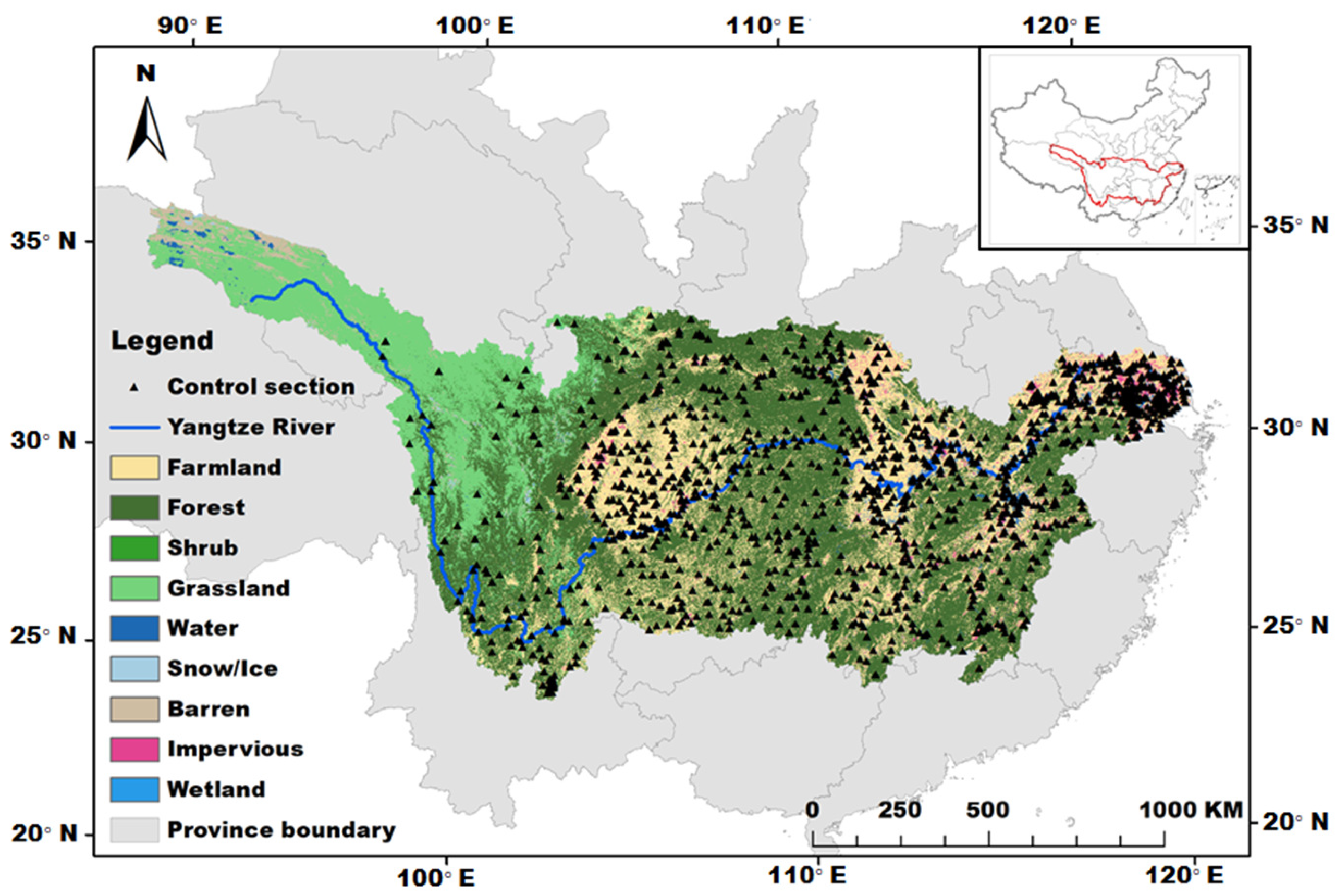
2.1. Study Area
2.2. Data
2.2.1. Water Quality Monitoring Data
2.2.2. Digital Elevation Model Data
2.2.3. China Land Cover Dataset
2.2.4. WorldPop Data
2.2.5. Point of Interest (POI) Data
2.2.6. Meteorological Data
3. Methods
3.1. Geographically Weighted Random Forest Model
3.2. The Variable Importance Measurement (VIM)
3.3. Model Evaluation
4. Results and Analysis
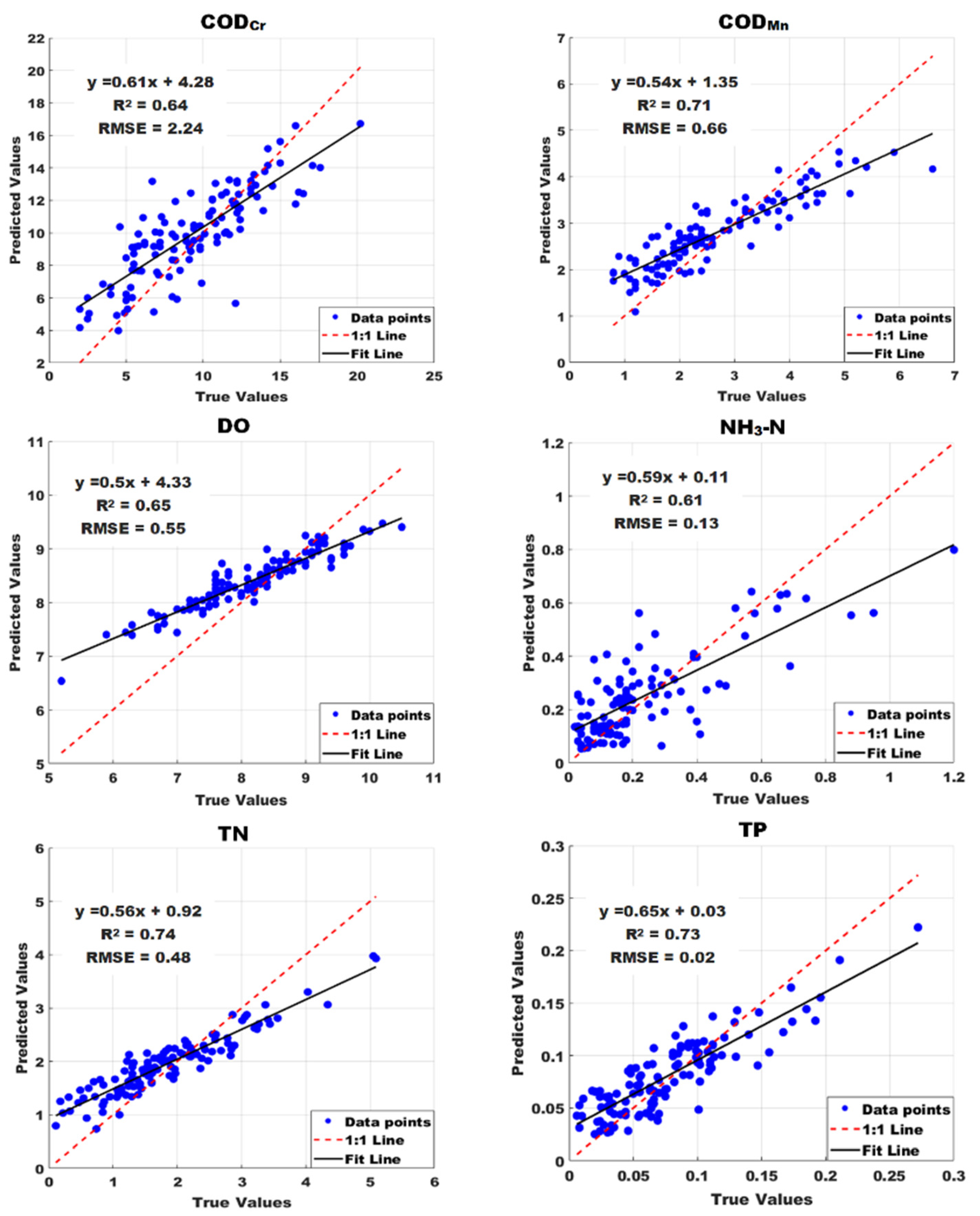
4.1. Water Quality Prediction Model Assessment
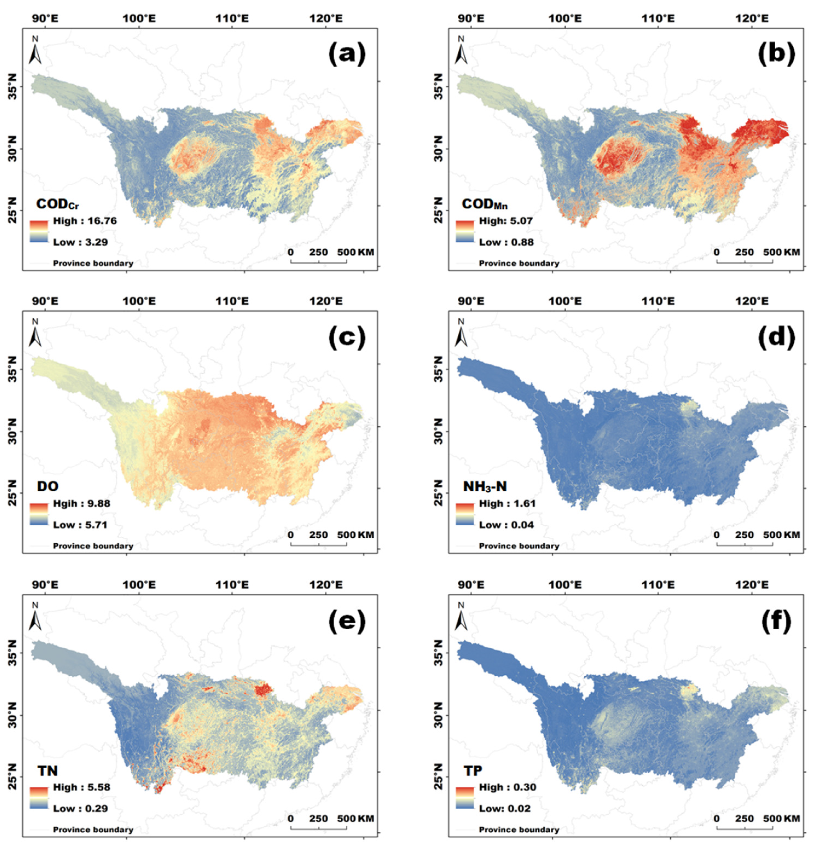
4.2. Mapping the Yangtze River Water Quality Indicators
4.3. An Analysis of Factors Influencing Water Quality
4.3.1. Importance Analysis
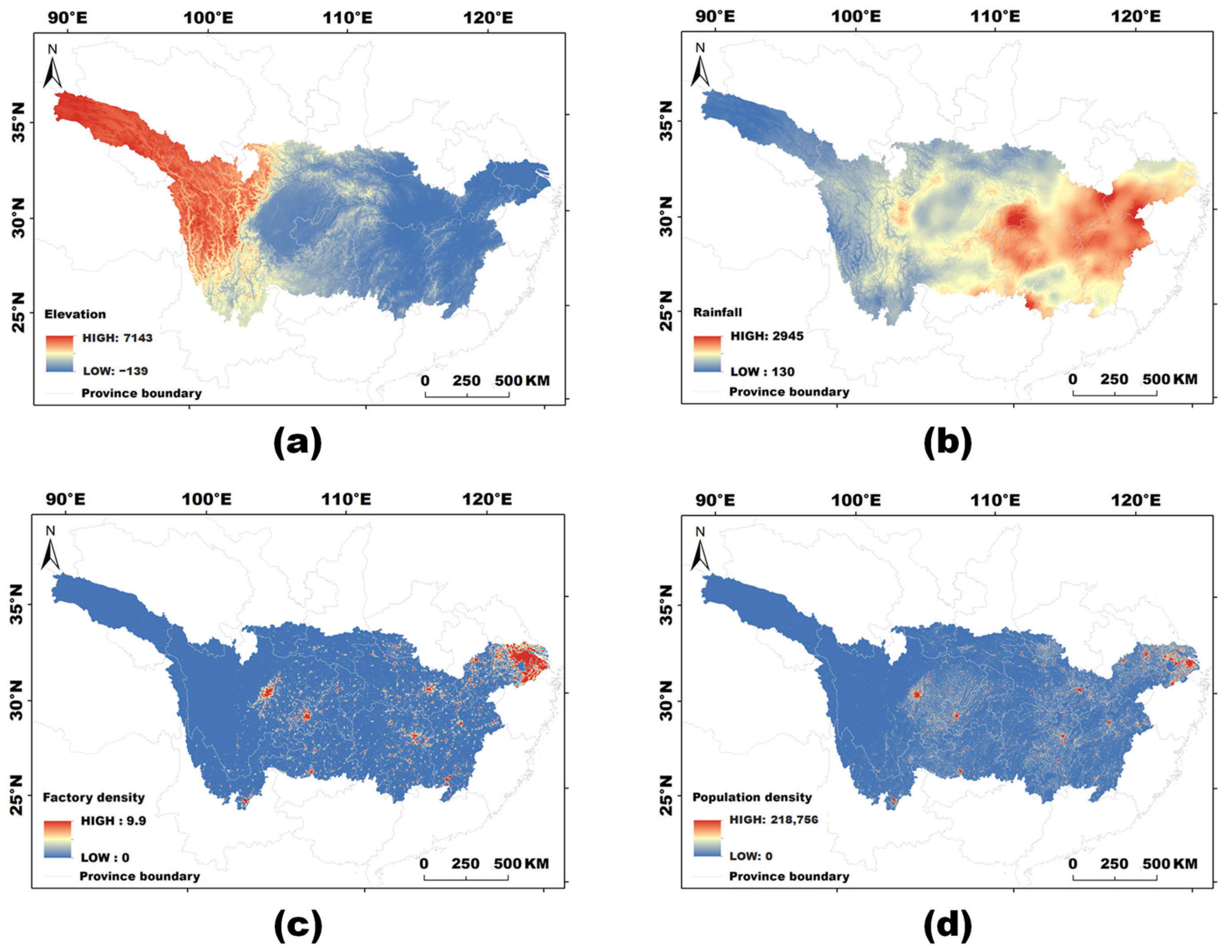
4.3.2. Spatial Distribution Analysis of Key Influencing Factors
5. Discussion
6. Conclusions
Author Contributions
Funding
Data Availability Statement
Conflicts of Interest
Appendix A

| Section Code | CODCr (mg/L) | CODMn (mg/L) | DO (mg/L) | NH3-N (mg/L) | TN (mg/L) | TP (mg/L) |
|---|---|---|---|---|---|---|
| 0001 | 13.3 | 5.4 | 7.4 | 0.16 | 1.77 | 0.115 |
| 0002 | 11.4 | 3.9 | 7.9 | 0.19 | 1.92 | 0.101 |
| 0003 | 11 | 2.2 | 7.6 | 0.14 | 1.78 | 0.092 |
| 0004 | 8.8 | 2.6 | 8.6 | 0.13 | 2.16 | 0.117 |
| 0005 | 13.5 | 3.2 | 6.5 | 0.5 | 3.01 | 0.116 |
| 0006 | 8.2 | 2.2 | 8.2 | 0.12 | 2.08 | 0.084 |
| 0007 | 13.4 | 4.2 | 8.6 | 0.18 | 2.51 | 0.068 |
| 0008 | 14.8 | 4.2 | 7.9 | 0.47 | 2.19 | 0.104 |
| 0009 | 8.4 | 2 | 7.8 | 0.07 | 2.35 | 0.088 |
| 0010 | 6.8 | 2.3 | 8.4 | 0.08 | 2.14 | 0.102 |
| 0011 | 12.8 | 4 | 6.3 | 0.15 | 1.84 | 0.102 |
| 0012 | 11 | 2.6 | 6.5 | 0.23 | 2.01 | 0.16 |
| 0013 | 13.6 | 4.6 | 7 | 0.26 | 2.39 | 0.157 |
| 0014 | 12.4 | 3 | 7.8 | 0.26 | 2.26 | 0.16 |
| 0015 | 11.3 | 3.4 | 7.4 | 0.45 | 2.24 | 0.168 |
| 0016 | 11.7 | 2.7 | 8.3 | 0.19 | 1.93 | 0.088 |
| 0017 | 18.3 | 4.9 | 7.8 | 0.69 | 2.48 | 0.156 |
| 0018 | 10.9 | 3 | 8.3 | 0.82 | 2.43 | 0.106 |
| 0019 | 17.7 | 4.8 | 7.6 | 0.34 | 1.88 | 0.073 |
| 0020 | 11.8 | 2.5 | 10.2 | 0.11 | 1.79 | 0.087 |
| 0021 | 9.1 | 2.4 | 7.5 | 0.16 | 1.84 | 0.101 |
| 0022 | 10 | 2.7 | 7 | 0.45 | 2.58 | 0.13 |
| 0023 | 8.2 | 2.5 | 7.2 | 0.24 | 2.33 | 0.111 |
| 0024 | 9.4 | 2.4 | 7.7 | 0.14 | 1.7 | 0.099 |
| 0025 | 18.9 | 5 | 7.8 | 0.2 | 1.24 | 0.044 |
| 0026 | 17.8 | 4.3 | 8.1 | 0.2 | 1.03 | 0.055 |
| 0027 | 7.8 | 2.1 | 8.1 | 0.34 | 1.98 | 0.074 |
| 0028 | 9.7 | 3.5 | 8.2 | 0.33 | 1.9 | 0.057 |
| 0029 | 10 | 2.7 | 8 | 0.43 | 2.43 | 0.08 |
| 0030 | 7.2 | 2.4 | 8.2 | 0.16 | 1.34 | 0.061 |
| 0031 | 5.8 | 2.2 | 9.4 | 0.15 | 1.52 | 0.038 |
| 0032 | 9.8 | 3.2 | 9 | 0.49 | 1.8 | 0.124 |
| 0033 | 11.4 | 4 | 7.3 | 0.57 | 2.66 | 0.099 |
| 0034 | 12.3 | 2.8 | 7.9 | 0.26 | 1.83 | 0.064 |
| 0035 | 8.6 | 2.6 | 7.8 | 0.14 | 2.02 | 0.061 |
| 0036 | 12.8 | 2.3 | 8.7 | 0.09 | 1.75 | 0.064 |
| 0037 | 13.3 | 3.7 | 8.2 | 0.09 | 0.9 | 0.045 |
| 0038 | 5.8 | 1.5 | 10 | 0.03 | 1.18 | 0.024 |
| 0039 | 8.4 | 2.5 | 8.5 | 0.04 | 0.95 | 0.037 |
| 0040 | 6.2 | 1.9 | 9.6 | 0.04 | 1.38 | 0.032 |
References
- Xiao, J.; Gao, D.; Zhang, H.; Shi, H.; Chen, Q.; Li, H.; Ren, X.; Chen, Q. Water quality assessment and pollution source apportionment using multivariate statistical techniques: A case study of the Laixi River Basin, China. Environ. Monit. Assess. 2023, 195, 287. [Google Scholar] [CrossRef] [PubMed]
- Chen, S.; Fang, M.; Zhuang, D. Spatial non-stationarity and heterogeneity of metropolitan housing prices: The case of Guangzhou, China. IOP Conf. Ser. Mater. Sci. Eng. 2019, 563, 42008. [Google Scholar] [CrossRef]
- Comber, A. Hyper-local geographically weighted regression: Extending GWR through local model selection and local bandwidth optimization. J. Spat. Int. Sci. 2018, 63–84. [Google Scholar] [CrossRef]
- Wang, F.; Wang, Y.; Zhang, K.; Hu, M.; Weng, Q.; Zhang, H. Spatial heterogeneity modeling of water quality based on random forest regression and model interpretation. Environ. Res. 2021, 202, 111660. [Google Scholar] [CrossRef]
- Masoumi, F.; Afshar, A.; Palatkaleh, S.T. Selective withdrawal optimization in river-reservoir systems; trade-offs between maximum allowable receiving waste load and water quality criteria enhancement. Environ. Monit. Assess. 2016, 188, 390. [Google Scholar] [CrossRef]
- Jeznach, L.C.; Jones, C.; Matthews, T.; Tobiason, J.E.; Ahlfeld, D.P. A framework for modeling contaminant impacts on reservoir water quality. J. Hydrol. 2016, 537, 322–333. [Google Scholar] [CrossRef]
- Sadeghian, A.; Chapra, S.C.; Hudson, J.; Wheater, H.; Lindenschmidt, K. Improving in-lake water quality modeling using variable chlorophyll a/algal biomass ratios. Environ. Modell. Softw. 2018, 101, 73–85. [Google Scholar] [CrossRef]
- Yazdi, J.; Moridi, A. Interactive Reservoir-Watershed Modeling Framework for Integrated Water Quality Management. Water Resour. Manag. 2017, 31, 2105–2125. [Google Scholar] [CrossRef]
- Costa, C.M.D.S.; Leite, I.R.; Almeida, A.K.; de Almeida, I.K. Choosing an appropriate water quality model—A review. Environ. Monit. Assess. 2021, 193, 38. [Google Scholar] [CrossRef]
- Ye, T.; Zhao, N.; Yang, X.; Ouyang, Z.; Liu, X.; Chen, Q.; Hu, K.; Yue, W.; Qi, J.; Li, Z.; et al. Improved population mapping for China using remotely sensed and points-of-interest data within a random forests model. Sci. Total Environ. 2019, 658, 936–946. [Google Scholar] [CrossRef]
- You, H.; Yang, J.; Xue, B.; Xiao, X.; Xia, J.; Jin, C.; Li, X. Spatial evolution of population change in Northeast China during 1992–2018. Sci. Total Environ. 2021, 776, 146023. [Google Scholar] [CrossRef]
- Chen, Y.; Wu, G.; Ge, Y.; Xu, Z. Mapping Gridded Gross Domestic Product Distribution of China Using Deep Learning with Multiple Geospatial Big Data. IEEE J. Sel. Top. Appl. Earth Observ. Remote Sens. 2022, 15, 1791–1802. [Google Scholar] [CrossRef]
- Zhong, L.; Liu, X.; Ao, J. Spatiotemporal dynamics evaluation of pixel-level gross domestic product, electric power consumption, and carbon emissions in countries along the belt and road. Energy 2022, 239, 121841. [Google Scholar] [CrossRef]
- Khan, S.N.; Li, D.; Maimaitijiang, M. A Geographically Weighted Random Forest Approach to Predict Corn Yield in the US Corn Belt. Remote Sens. 2022, 14, 2843. [Google Scholar] [CrossRef]
- Burigato Costa, C.M.D.S.; Da Silva Marques, L.; Almeida, A.K.; Leite, I.R.; de Almeida, I.K. Applicability of water quality models around the world—A review. Environ. Sci. Pollut. Res. 2019, 26, 36141–36162. [Google Scholar] [CrossRef]
- Rajaee, T.; Khani, S.; Ravansalar, M. Artificial intelligence-based single and hybrid models for prediction of water quality in rivers: A review. Chemom. Intell. Lab. Syst. 2020, 200, 103978. [Google Scholar] [CrossRef]
- Draidi Areed, W.; Price, A.; Arnett, K.; Mengersen, K. Spatial statistical machine learning models to assess the relationship between development vulnerabilities and educational factors in children in Queensland, Australia. Bmc Public Health. 2022, 22, 2232. [Google Scholar] [CrossRef]
- Lotfata, A.; Georganos, S.; Kalogirou, S.; Helbich, M. Ecological Associations between Obesity Prevalence and Neighborhood Determinants Using Spatial Machine Learning in Chicago, Illinois, USA. ISPRS Int. J. Geo-Inf. 2022, 11, 550. [Google Scholar] [CrossRef]
- Liao, H.; Sun, W. Forecasting and Evaluating Water Quality of Chao Lake based on an Improved Decision Tree Method. Procedia Environ. Sci. 2010, 2, 970–979. [Google Scholar] [CrossRef]
- Zare, A.H. Evaluation of multivariate linear regression and artificial neural networks in prediction of water quality parameters. J. Environ. Health Sci. Eng. 2014, 12, 40. [Google Scholar] [CrossRef]
- Liu, J.; Yu, C.; Hu, Z.; Zhao, Y.; Bai, Y.; Xie, M.; Luo, J. Accurate Prediction Scheme of Water Quality in Smart Mariculture with Deep Bi-S-SRU Learning Network. IEEE Access 2020, 8, 24784–24798. [Google Scholar] [CrossRef]
- Li, L.; Jiang, P.; Xu, H.; Lin, G.; Guo, D.; Wu, H. Water quality prediction based on recurrent neural network and improved evidence theory: A case study of Qiantang River, China. Environ. Sci. Pollut. Res. Int. 2019, 26, 19879–19896. [Google Scholar] [CrossRef] [PubMed]
- Liu, P.; Wang, J.; Sangaiah, A.; Xie, Y.; Yin, X. Analysis and Prediction of Water Quality Using LSTM Deep Neural Networks in IoT Environment. Sustainability 2019, 11, 2058. [Google Scholar] [CrossRef]
- Wang, X.; Qiao, M.; Li, Y.; Tavares, A.; Qiao, Q.; Liang, Y. Deep-Learning-Based Water Quality Monitoring and Early Warning Methods: A Case Study of Ammonia Nitrogen Prediction in Rivers. Electronics 2023, 12, 4645. [Google Scholar] [CrossRef]
- Georganos, S.; Grippa, T.; Niang Gadiaga, A.; Linard, C.; Lennert, M.; Vanhuysse, S.; Mboga, N.; Wolff, E.; Kalogirou, S. Geographical random forests: A spatial extension of the random forest algorithm to address spatial heterogeneity in remote sensing and population modelling. Geocarto Int. 2021, 36, 121–136. [Google Scholar] [CrossRef]
- Quiñones, S.; Goyal, A.; Ahmed, Z.U. Geographically weighted machine learning model for untangling spatial heterogeneity of type 2 diabetes mellitus (T2D) prevalence in the USA. Sci. Rep. 2021, 11, 6955. [Google Scholar]
- Ren, Y.; Yuan, W.; Zhang, B.; Wang, S. Does improvement of environmental efficiency matter in reducing carbon emission intensity? Fresh evidence from 283 prefecture-level cities in China. J. Clean. Prod. 2022, 373, 133878. [Google Scholar] [CrossRef]
- Huang, J.; Huang, Y.; Pontius Jr, R.G.; Zhang, Z. Geographically weighted regression to measure spatial variations in correlations between water pollution versus land use in a coastal watershed. Ocean. Coast. Manag. 2015, 103, 14–24. [Google Scholar] [CrossRef]
- Mainali, J.; Chang, H.; Parajuli, R. Stream distance-based geographically weighted regression for exploring watershed characteristics and water quality relationships. Ann. Am. Assoc. Geogr. 2023, 113, 390–408. [Google Scholar] [CrossRef]
- Grekousis, G.; Feng, Z.; Marakakis, I.; Lu, Y.; Wang, R. Ranking the importance of demographic, socioeconomic, and underlying health factors on US COVID-19 deaths: A geographical random forest approach. Health Place 2022, 74, 102744. [Google Scholar] [CrossRef]
- Chen, Y.; Zang, L.; Shen, G.; Liu, M.; Du, W.; Fei, J.; Yang, L.; Chen, L.; Wang, X.; Liu, W.; et al. Resolution of the Ongoing Challenge of Estimating Nonpoint Source Neonicotinoid Pollution in the Yangtze River Basin Using a Modified Mass Balance Approach. Environ. Sci. Technol. 2019, 53, 2539–2548. [Google Scholar] [CrossRef] [PubMed]
- Chen, T.; Wang, Y.; Gardner, C.; Wu, F. Threats and protection policies of the aquatic biodiversity in the Yangtze River. J. Nat. Conserv. 2020, 58, 125931. [Google Scholar] [CrossRef]
- Li, X.; Mander, Ü.; Ma, Z.; Jia, Y. Water Quality Problems and Potential for Wetlands as Treatment Systems in the Yangtze River Delta, China. Wetlands 2009, 29, 1125–1132. [Google Scholar] [CrossRef]
- Di, Z.; Chang, M.; Guo, P.; Li, Y.; Chang, Y. Using Real-Time Data and Unsupervised Machine Learning Techniques to Study Large-Scale Spatio–Temporal Characteristics of Wastewater Discharges and their Influence on Surface Water Quality in the Yangtze River Basin. Water 2019, 11, 1268. [Google Scholar] [CrossRef]
- Liu, S.; Fu, R.; Liu, Y.; Suo, C. Spatiotemporal variations of water quality and their driving forces in the Yangtze River Basin, China, from 2008 to 2020 based on multi-statistical analyses. Environ. Sci. Pollut. Res. 2022, 29, 69388–69401. [Google Scholar] [CrossRef]
- Huang, J.; Zhang, Y.; Bing, H.; Peng, J.; Dong, F.; Gao, J.; Arhonditsis, G.B. Characterizing the river water quality in China: Recent progress and on-going challenges. Water Res. 2021, 201, 117309. [Google Scholar] [CrossRef]
- Di, Z.; Chang, M.; Guo, P. Water Quality Evaluation of the Yangtze River in China Using Machine Learning Techniques and Data Monitoring on Different Time Scales. Water 2019, 11, 339. [Google Scholar] [CrossRef]
- Duan, W.; He, B.; Chen, Y.; Zou, S.; Wang, Y.; Nover, D.; Chen, W.; Yang, G. Identification of long-term trends and seasonality in high-frequency water quality data from the Yangtze River basin, China. PLoS ONE 2018, 13, e0188889. [Google Scholar] [CrossRef]
- Lu, J.; Gu, J.; Han, J.; Xu, J.; Liu, Y.; Jiang, G.; Zhang, Y. Evaluation of Spatiotemporal Patterns and Water Quality Conditions Using Multivariate Statistical Analysis in the Yangtze River, China. Water 2023, 15, 3242. [Google Scholar] [CrossRef]
- Yao, R.; Wang, L.; Gui, X.; Zheng, Y.; Zhang, H.; Huang, X. Urbanization Effects on Vegetation and Surface Urban Heat Islands in China’s Yangtze River Basin. Remote Sens. 2017, 9, 540. [Google Scholar] [CrossRef]
- Yang, X.; Meng, F.; Fu, P.; Zhang, Y.; Liu, Y. Spatiotemporal change and driving factors of the Eco-Environment quality in the Yangtze River Basin from 2001 to 2019. Ecol. Indic. 2021, 131, 108214. [Google Scholar] [CrossRef]
- Yang, P.; Xia, J.; Luo, X.; Meng, L.; Zhang, S.; Cai, W.; Wang, W. Impacts of climate change-related flood events in the Yangtze River Basin based on multi-source data. Atmos. Res. 2021, 263, 105819. [Google Scholar] [CrossRef]
- Li, Y.; Yan, D.; Peng, H.; Xiao, S. Evaluation of precipitation in CMIP6 over the Yangtze River Basin. Atmos. Res. 2021, 253, 105406. [Google Scholar] [CrossRef]
- Qu, S.; Wang, L.; Lin, A.; Yu, D.; Yuan, M.; Li, C. Distinguishing the impacts of climate change and anthropogenic factors on vegetation dynamics in the Yangtze River Basin, China. Ecol. Indic. 2020, 108, 105724. [Google Scholar] [CrossRef]
- Smith, B.; Sandwell, D. Accuracy and resolution of shuttle radar topography mission data. Geophys. Res. Lett. 2003, 30, 1467. [Google Scholar] [CrossRef]
- Yang, J.; Huang, X. The 30 m annual land cover dataset and its dynamics in China from 1990 to 2019. Earth Syst. Sci. Data 2021, 13, 3907–3925. [Google Scholar] [CrossRef]
- Calka, B.; Nowak Da Costa, J.; Bielecka, E. Fine scale population density data and its application in risk assessment. Geomat. Nat. Hazards Risk 2017, 8, 1440–1455. [Google Scholar] [CrossRef]
- Tatem, A.J. WorldPop, open data for spatial demography. Sci. Data 2017, 4, 170004. [Google Scholar] [CrossRef]
- Bai, Z.; Wang, J.; Wang, M.; Gao, M.; Sun, J. Accuracy Assessment of Multi-Source Gridded Population Distribution Datasets in China. Sustainability 2018, 10, 1363. [Google Scholar] [CrossRef]
- Stevens, F.R.; Gaughan, A.E.; Linard, C.; Tatem, A.J. Disaggregating census data for population mapping using random forests with remotely-sensed and ancillary data. PLoS ONE 2015, 10, e0107042. [Google Scholar] [CrossRef] [PubMed]
- Trigg, M.A.; Birch, C.E.; Neal, J.C.; Bates, P.D.; Smith, A.; Sampson, C.C.; Yamazaki, D.; Hirabayashi, Y.; Pappenberger, F.; Dutra, E.; et al. The credibility challenge for global fluvial flood risk analysis. Environ. Res. Lett. 2016, 11, 94014. [Google Scholar] [CrossRef]
- Mohanty, M.P.; Simonovic, S.P. Understanding dynamics of population flood exposure in Canada with multiple high-resolution population datasets. Sci. Total Environ. 2021, 759, 143559. [Google Scholar] [CrossRef] [PubMed]
- Wang, J.; Wei, J.; Zhang, W.; Liu, Z.; Du, X.; Liu, W.; Pan, K. High-resolution temporal and spatial evolution of carbon emissions from building operations in Beijing. J. Clean. Prod. 2022, 376, 134272. [Google Scholar] [CrossRef]
- Guo, B.; Zhang, J.; Meng, X.; Xu, T.; Song, Y. Long-term spatio-temporal precipitation variations in China with precipitation surface interpolated by ANUSPLIN. Sci. Rep. 2020, 10, 81. [Google Scholar] [CrossRef] [PubMed]
- Danladi Bello, A.; Hashim, N.; Mohd Haniffah, M. Predicting Impact of Climate Change on Water Temperature and Dissolved Oxygen in Tropical Rivers. Climate 2017, 5, 58. [Google Scholar] [CrossRef]
- Quevedo-Castro, A.; Bustos-Terrones, Y.A.; Bandala, E.R.; Loaiza, J.G.; Rangel-Peraza, J.G. Modeling the effect of climate change scenarios on water quality for tropical reservoirs. J. Environ. Manag. 2022, 322, 116137. [Google Scholar] [CrossRef]
- Jerves-Cobo, R.; Forio, M.A.E.; Lock, K.; Van Butsel, J.; Pauta, G.; Cisneros, F.; Nopens, I.; Goethals, P.L.M. Biological water quality in tropical rivers during dry and rainy seasons: A model-based analysis. Ecol. Indic. 2020, 108, 105769. [Google Scholar] [CrossRef]
- Luo, Y.; Yan, J.; McClure, S.C.; Li, F. Socioeconomic and environmental factors of poverty in China using geographically weighted random forest regression model. Environ. Sci. Pollut. Res. 2022, 29, 33205–33217. [Google Scholar] [CrossRef]
- Ishwaran, H. Variable importance in binary regression trees and forests. Electron. J. Stat. 2007, 1, 519–537. [Google Scholar] [CrossRef]
- Strobl, C.; Boulesteix, A.L.; Zeileis, A.; Hothorn, T. Bias in random forest variable importance measures: Illustrations, sources and a solution. BMC Bioinform. 2007, 8, 25. [Google Scholar] [CrossRef]
- Strobl, C.; Boulesteix, A.; Kneib, T.; Augustin, T.; Zeileis, A. Conditional variable importance for random forests. BMC Bioinform. 2008, 9, 307. [Google Scholar] [CrossRef] [PubMed]
- Cai, H.; Lam, N.S.N.; Qiang, Y.; Zou, L.; Correll, R.M.; Mihunov, V. A synthesis of disaster resilience measurement methods and indices. Int. J. Disaster Risk Reduct. 2018, 31, 844–855. [Google Scholar] [CrossRef]
- Sakaa, B.; Elbeltagi, A.; Boudibi, S.; Chaffai, H.; Islam, A.; Cimusa Kulimushi, L.; Choudhari, P.P.; HANI, A.; Brouziyne, Y.; Wong, Y.J. Water quality index modeling using random forest and improved SMO algorithm for support vector machine in Saf-Saf river basin. Environ. Sci. Pollut. Res. 2022, 29, 48491–48508. [Google Scholar] [CrossRef] [PubMed]
- Ren, L.; Huang, J.; Wang, B.; Wang, H.; Gong, R.; Hu, Z. Effects of temperature on the growth and competition between Microcystis aeruginosa and Chlorella pyrenoidosa with different phosphorus availabilities. Desalination Water Treat. 2021, 241, 87–111. [Google Scholar] [CrossRef]
- Koç, T. Bandwidth Selection in Geographically Weighted Regression Models via Information Complexity Criteria. J. Math. 2022, 2022, 1527407. [Google Scholar] [CrossRef]
- Xu, X.; Zhu, M.; Zhou, L.; Ma, M.; Heng, J.; Lu, L.; Qu, W.; Xu, Z. The impact of slope and rainfall on the contaminant transport from mountainous groundwater to the lowland surface water. Front. Environ. Sci. 2024, 12, 1343903. [Google Scholar] [CrossRef]
- Qin, B.; Xu, P.; Wu, Q.; Luo, L.; Zhang, Y. Environmental issues of Lake Taihu, China. Hydrobiologia 2007, 581, 3–14. [Google Scholar] [CrossRef]
- Li, S.; Peng, S.; Jin, B.; Zhou, J.; Li, Y. Multi-scale relationship between land use/land cover types and water quality in different pollution source areas in Fuxian Lake Basin. Peerj 2019, 7, e7283. [Google Scholar] [CrossRef]
- Shi, P.; Zhang, Y.; Song, J.; Li, P.; Wang, Y.; Zhang, X.; Li, Z.; Bi, Z.; Zhang, X.; Qin, Y.; et al. Response of nitrogen pollution in surface water to land use and social-economic factors in the Weihe River watershed, northwest China. Sustain. Cities Soc. 2019, 50, 101658. [Google Scholar] [CrossRef]


| Category | Data | Role in Model Training | Spatial Resolution |
|---|---|---|---|
| Water quality data | Control section unit data | Spatial range represented by water quality monitoring data | / |
| Water quality monitoring | Monitoring water quality | / | |
| Auxiliary data | Digital elevation model | Characterizing the influence of topography on the water quality | 30 m |
| China Land Cover Dataset | Filtering out specific land cover and characterizing the land cover impact on the water quality | 30 m | |
| WorldPop data | Characterizing the influence of population on the water quality | 100 m | |
| Point of interest data | Characterizing the influence of factory distribution on the water quality | 30 m | |
| Meteorological data | Characterizing the influence of temperature and rainfall on the water quality | 1 km |
| Water Quality Indicator | Unit | Description |
|---|---|---|
| Chemical oxygen demand (CODCr) | mg/L | The amount of oxygen needed to oxidize the organic matter in water. |
| Permanganate index (CODMn) | mg/L | Assesses the impact of organic pollutants on ecosystems and the concentration of organic pollutants in the water. |
| Dissolved oxygen (DO) | mg/L | The oxygen content in water, obtained by assessing the biological viability of water bodies. |
| Ammonia nitrogen (NH3-N) | mg/L | Ammonia nitrogen concentration in water, obtained by assessing the eutrophication of water bodies. |
| Total nitrogen (TN) | mg/L | Total nitrogen concentration in water, including ammonia nitrogen, nitrate nitrogen, organic nitrogen, etc. |
| Total phosphorus (TP) | mg/L | Total phosphorus concentration in water, including dissolved and non-dissolved phosphorus. |
Disclaimer/Publisher’s Note: The statements, opinions and data contained in all publications are solely those of the individual author(s) and contributor(s) and not of MDPI and/or the editor(s). MDPI and/or the editor(s) disclaim responsibility for any injury to people or property resulting from any ideas, methods, instructions or products referred to in the content. |
© 2025 by the authors. Licensee MDPI, Basel, Switzerland. This article is an open access article distributed under the terms and conditions of the Creative Commons Attribution (CC BY) license (https://creativecommons.org/licenses/by/4.0/).
Share and Cite
Deng, F.; Liu, W.; Sun, M.; Xu, Y.; Wang, B.; Liu, W.; Yuan, Y.; Cui, L. Fine Estimation of Water Quality in the Yangtze River Basin Based on a Geographically Weighted Random Forest Regression Model. Remote Sens. 2025, 17, 731. https://doi.org/10.3390/rs17040731
Deng F, Liu W, Sun M, Xu Y, Wang B, Liu W, Yuan Y, Cui L. Fine Estimation of Water Quality in the Yangtze River Basin Based on a Geographically Weighted Random Forest Regression Model. Remote Sensing. 2025; 17(4):731. https://doi.org/10.3390/rs17040731
Chicago/Turabian StyleDeng, Fuliang, Wenhui Liu, Mei Sun, Yanxue Xu, Bo Wang, Wei Liu, Ying Yuan, and Lei Cui. 2025. "Fine Estimation of Water Quality in the Yangtze River Basin Based on a Geographically Weighted Random Forest Regression Model" Remote Sensing 17, no. 4: 731. https://doi.org/10.3390/rs17040731
APA StyleDeng, F., Liu, W., Sun, M., Xu, Y., Wang, B., Liu, W., Yuan, Y., & Cui, L. (2025). Fine Estimation of Water Quality in the Yangtze River Basin Based on a Geographically Weighted Random Forest Regression Model. Remote Sensing, 17(4), 731. https://doi.org/10.3390/rs17040731