Identification and Analysis of Wind Shear Within the Transiting Frontal System at Xining International Airport Using Lidar

Abstract

The principal factor contributing to the restricted accuracy of wind shear detection resides in the rapid oscillations of the wind field and the intricate characteristics of wind shear. The abrupt alterations in wind speed and direction over a short span pose a formidable challenge for conventional detection techniques to precisely capture and expeditiously analyze this phenomenon. In this study, three algorithms were employed to analyze wind shear within the frontal system at Xining International Airport on 5 April 2023, and the same analytical approach was applied to three additional paradigmatic cases. Initially, the slope characteristics of the Lidar signal were utilized to ascertain the existence and intensity of wind shear by assessing the rate of variation of the wind field parameters along a specific trajectory. Secondly, the S-factor algorithm was applied to detect wind shear. This algorithm revolves around particular mathematical relationships and statistical measures within the wind field data. By taking into account multiple variables and their mutual interactions, an S-factor value was computed to signify the strength of wind shear. Furthermore, an enhanced F-factor algorithm was found upon scrutinizing the identical wind field data, as they all detected a substantial intensification in wind shear intensity prior to and after the issuance of the voice report. This evinces that despite the differences in sensitivity, all three algorithms are able to capture the general trend of wind shear fluctuations during the passage of the frontal system.

1. Introduction

Low-level wind shear, precisely defined as a rapid and substantial variation in wind direction or speed within an altitude range below 600 m, poses a notably significant threat to aircraft operations during the critical take-off and landing phases [1]. This is primarily attributable to its inherently short temporal span, highly heterogeneous and variable manifestations, and formidable and potentially catastrophic destructive potential [2]. When an aircraft encounters intense low-level wind shear, it tends to experience instantaneous and significant alterations in lift and altitude [3]. Such abrupt changes can exert a profound and adverse impact on flight mechanics, thereby substantially increasing the likelihood and risk of a catastrophic accident [4,5,6]. Consequently, this perilous meteorological phenomenon has been metaphorically referred to as the “invisible plane assassin” within the aviation field [7]. A multitude of meteorological elements and factors, including fronts that demarcate the boundaries between disparate air masses with distinct characteristics, downbursts representing powerful and concentrated downdrafts of air, low-level rapids denoting rapid and frequently turbulent wind currents at lower altitudes, and turbulence characterized by disordered and erratic air motions, all actively contribute to the occurrence of low-level wind shear [8,9,10].

Wind Lidar, a state-of-the-art wind measurement instrument, utilizes aerosol particles as tracers and employs the Doppler effect to retrieve the atmospheric wind field [11]. Compared with traditional weather radars and wind profilers, it demonstrates superior accuracy and higher resolution in wind field detection [12]. As Wind Lidar technology has been continuously evolving, its application in wind shear detection has been steadily advancing and approaching a stage of greater maturity. The prevalent scanning modalities of Lidar include the Plan Position Indicator (PPI), the Range Height Indicator (RHI), Doppler Beam Scanning (DBS), and Slide Path Scanning (SP) [13,14]. Each of these scanning modalities is accompanied by its own specific set of wind shear detection algorithms. For example, the slope detection, S-factor, F-factor, and modified F-factor algorithms are formulated based on the data acquired from the SP scanning mode [15,16,17]. Meanwhile, least-squares fitting and eight-neighbor algorithms are designed in line with the data obtained from the PPI scanning mode. Numerous factors contribute to the complexity and difficulty of accurately determining the actual intensity, location, and impact of wind shear on aircraft flights solely based on the local wind field [18]. The diversity of wind shear types, the significant differences and complex evolution processes among different wind shear phenomena, and the transient and dynamic characteristics of wind fields, all contribute to this complexity [19,20]. Consequently, it is of profound scientific significance for aviation safety to conduct a comprehensive evaluation and judgment of the influence of varying wind shear intensities on aircraft and to prudently select appropriate warning thresholds. This not only contributes to enhancing the safety and reliability of flight operations but also lays a critical foundation for the development and refinement of more effective wind shear prediction and mitigation strategies.

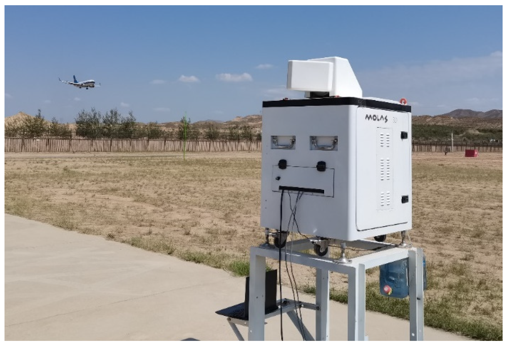
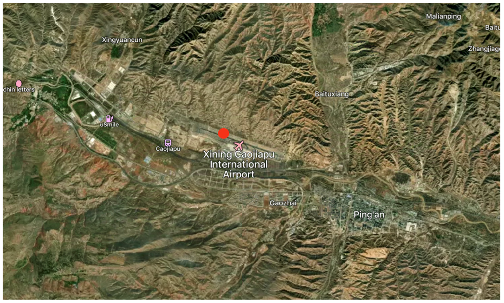
In several previous research studies, a limited number of scholars have utilized diverse algorithms and types of equipment to analyze the wind field data, resulting in disparate wind shear information [21,22,23]. This makes it difficult to compare information, such as the strength of wind shear, captured by different instruments. Given this situation, the current study centers on the process of low-level wind shear induced by a frontal system at Xining International Airport (located at 36°31′42′′N, 102°02′49′′E and with an altitude of 2184 m) in Qinghai Province, China. Based on the wind shear data obtained from Lidar observations in the Slide Path Scanning (SP) mode, a comprehensive analysis combined with three detection algorithms is carried out. Specifically, the slope detection algorithm, which takes advantage of the gradient characteristics of the wind field parameters, is employed to identify potential wind shear regions. The S-factor algorithm, which is based on specific mathematical relationships and statistical measures within the wind field data, is used to assess the likelihood of wind shear occurrence. Moreover, the modified F-factor algorithm, which is designed to improve the sensitivity and precision of wind shear detection, particularly in complex meteorological conditions, is applied. Furthermore, an in-depth exploration is conducted to clarify the characteristics of the wind field and the evolutionary process of wind shear under the influence of the frontal system. This entails a meticulous examination of the temporal and spatial variations of wind speed, direction, and other relevant parameters.

The paper is structured as follows. Section 2 is dedicated to the introduction of the utilized Lidar and its data processing method. Section 3 presents the weather background and aircraft voice reports during the passage of the frontal system at Xining International Airport. Section 4 is devoted to the analysis of wind fields and the results of wind shear detection using different algorithms. The final section (Section 5) offers the conclusions and discussions.

2. Equipment and Environment

2.1. Wind Lidar

The wind Lidar employed in this research utilizes aerosol particles as the detection target. A servo mechanism is implemented to govern the pitch and orientation of the emitted laser beam for the purpose of measuring the radial wind speed. Horizontally, the measurement range extends from 0 to 360°, and, vertically, it ranges from −10 to 90°, which allows it to detect the wind in all directions, as depicted in Figure 1. The high resolution in distance and wind speed enable Lidar to provide wind field data with enhanced precision. The pointing accuracy of 0.01° ensures that the Lidar can accurately point to the target measurement area and reduce the measurement error caused by pointing deviation. The maximum position update rate of 2 Hz means that the Lidar can update the measurement data every 0.5 s, and it can track dynamic changes of the wind field in time, which provides strong support for real-time wind field monitoring and early warning for fast-changing wind conditions, such as gusts, squall lines, etc. It has a good monitoring ability. The detailed technical parameters of the wind Lidar are presented in

Table 1. Parameters of the used 3D wind Lidar.

Technical Parameters	Technical Indicators
Wavelength	1550 nm ± 1 nm
Distance resolution	15 m/30 m
Blind spot width	140 m
Visual wind speed measurement range	−75 m/s~+75 m/s
Visual wind speed measurement accuracy	0.1 m/s
Number of distance gates	300
Horizontal scanning range (azimuth range)	360° × n
Vertical scanning range (pitch range)	−10°~90°
Angular resolution	0.002°
Pointing accuracy	0.01°
Maximum position update rate	2 Hz

.

2.2. Experimental Location

The Xining Airport is geographically located within the Huangshui River Basin, in the southeastern section of the Qilian Mountains and to the northeast of the Tibetan Plateau. Similarly to the situation where the water velocity escalates remarkably when flowing through a river canyon, the wind speed in the elongated and constricted terrain surrounding Xining Airport also witnesses an increase. According to statistical information from the airport, typically, the wind speed along the runway of Xining Airport is about 3–5 m per second greater than that in the upstream area of the Xining River and the downstream zone of the Ping’an District River. Concurrently, Xining Airport is encompassed by mountains, exhibiting a complex topographical configuration. To the north and south, it is bordered by mountains of diverse elevations. The mean altitude of the surrounding mountains surpasses 2500 m above sea level. As a result, the variations in wind direction and speed, the incidence of strong winds, and the manifestation of low-level wind shear are considerably affected by the distinctive geographical and natural environmental traits of this site (as depicted in Figure 2). The unique topography leads to complex wind direction patterns, thus increasing the probability of wind shear. The existence of lofty mountains in the proximity restricts the unobstructed movement of air masses, prompting them to accelerate and change direction suddenly, thus presenting potential perils to aviation activities. The specific topographical characteristics and their interaction with the prevailing meteorological circumstances necessitate an in-depth exploration to enhance the comprehension and mitigation of the associated risks.

The wind Lidar was installed on runway 11/29 of the airport, where runway 11 serves as the primary landing runway in the westward direction. The flight path of the aircraft during takeoff and landing is referred to as the glide path. The angle between the glide path and the runway is 6° during takeoff and 3° during landing. In view of the higher probability of wind shear hazard during landing, the aircraft’s glide path was scanned at an elevation angle of 3° in the direction of runway 11. To optimize the detection capability of the Lidar within the effective detection range, the Lidar was positioned near the landing point of runway 11 (with a bearing of 290°) along the main landing direction of the airport runway, as illustrated in Figure 3. Point O represents the landing point of the aircraft in the main landing direction, point L denotes the position of the radar, and the perpendicular distance of the radar from the runway centerline (OS) is 210 m. When the LAO angle is less than 30°, the radial velocity at point A in the direction L-A can be equated to the wind component at point A in the direction A-O, which is defined as the headwind velocity. The headwind velocity is designated as positive in the opposite direction of the aircraft velocity and negative in the same direction. During the execution of a glide path scan, the Lidar pitch and azimuth servos are manipulated such that the radar elevation and azimuth angles are adjusted concurrently to guarantee that the radar laser beam is constantly aligned with different locations on the glide path. For instance, by scanning along the direction from point A to point C, the headwind profile at different locations within the AC section can be acquired.

The wind Lidar regulates both the elevation and azimuth angles to conduct observations along the 3° elevation glide path; it takes about 60 rays to complete an SP scan. The rays that failed to satisfy the conditions (i.e., the angle between the laser beam and the glide path being less than 30°), those with a low signal-to-noise ratio, and those that exceeded the range were eliminated during data quality control, so the effective detection range is 1000–6000 m. Each SP scan encompassed approximately 28 valid rays. A complete SP scan could be accomplished in around 40 s, with an interval of approximately 6.5 min between two consecutive SP scans (about 320 s), resulting in approximately 220 sets of scans per day (where one complete SP scan constitutes one set).

3. Data Processing

3.1. Processing Flow

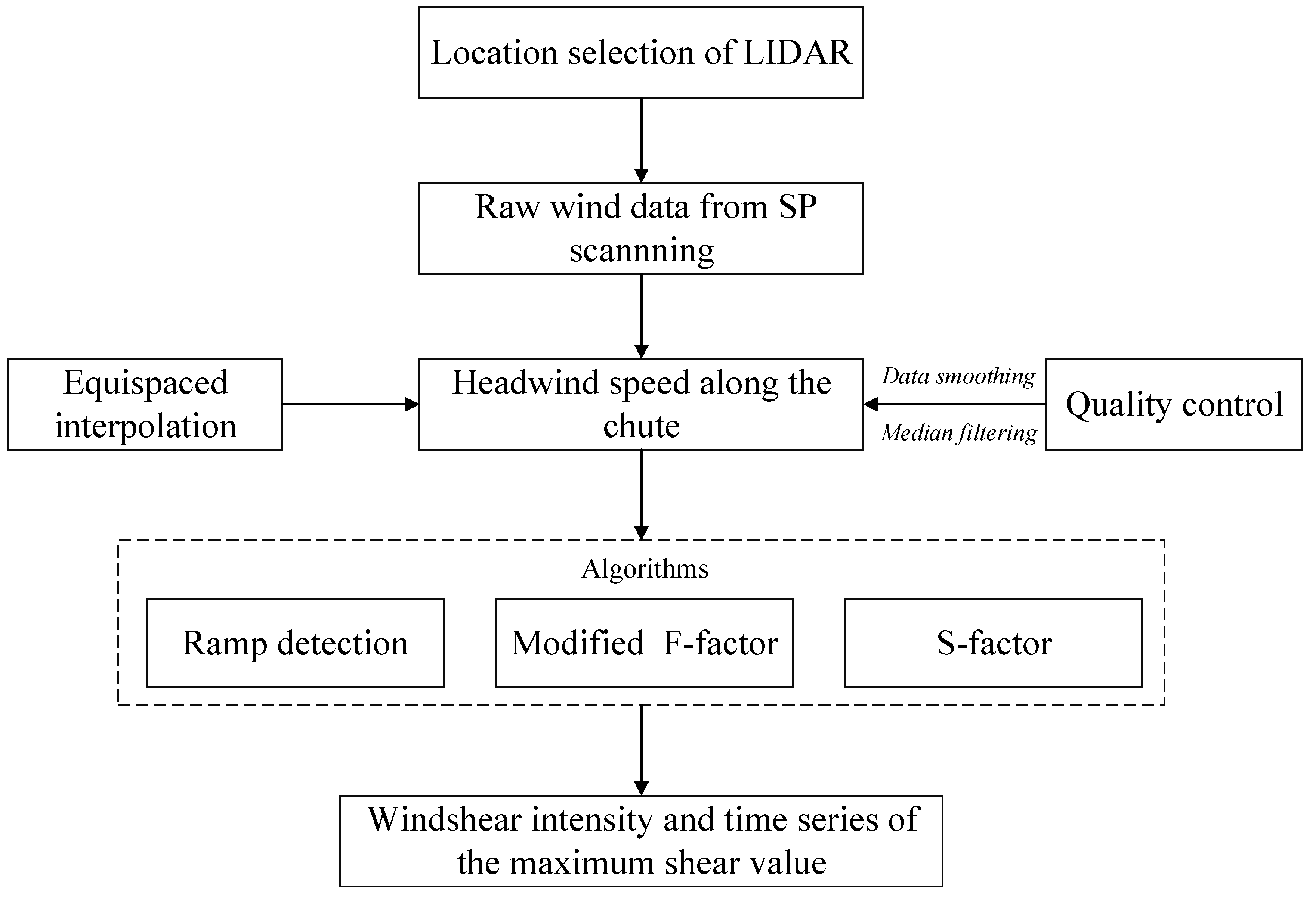
The headwind speed was extracted based on the data retrieved from SP scanning. Median filtering, data smoothing, and mean processing were all required to be implemented in order to obtain a high-quality headwind profile of the slope. Subsequently, the slope detection algorithm, the S-factor algorithm, and the modified F-factor algorithm were utilized to identify the wind shear intensity, and thereafter the maximum value was selected. The maximum value was extracted to construct a time series. The data processing flow is illustrated in Figure 4.

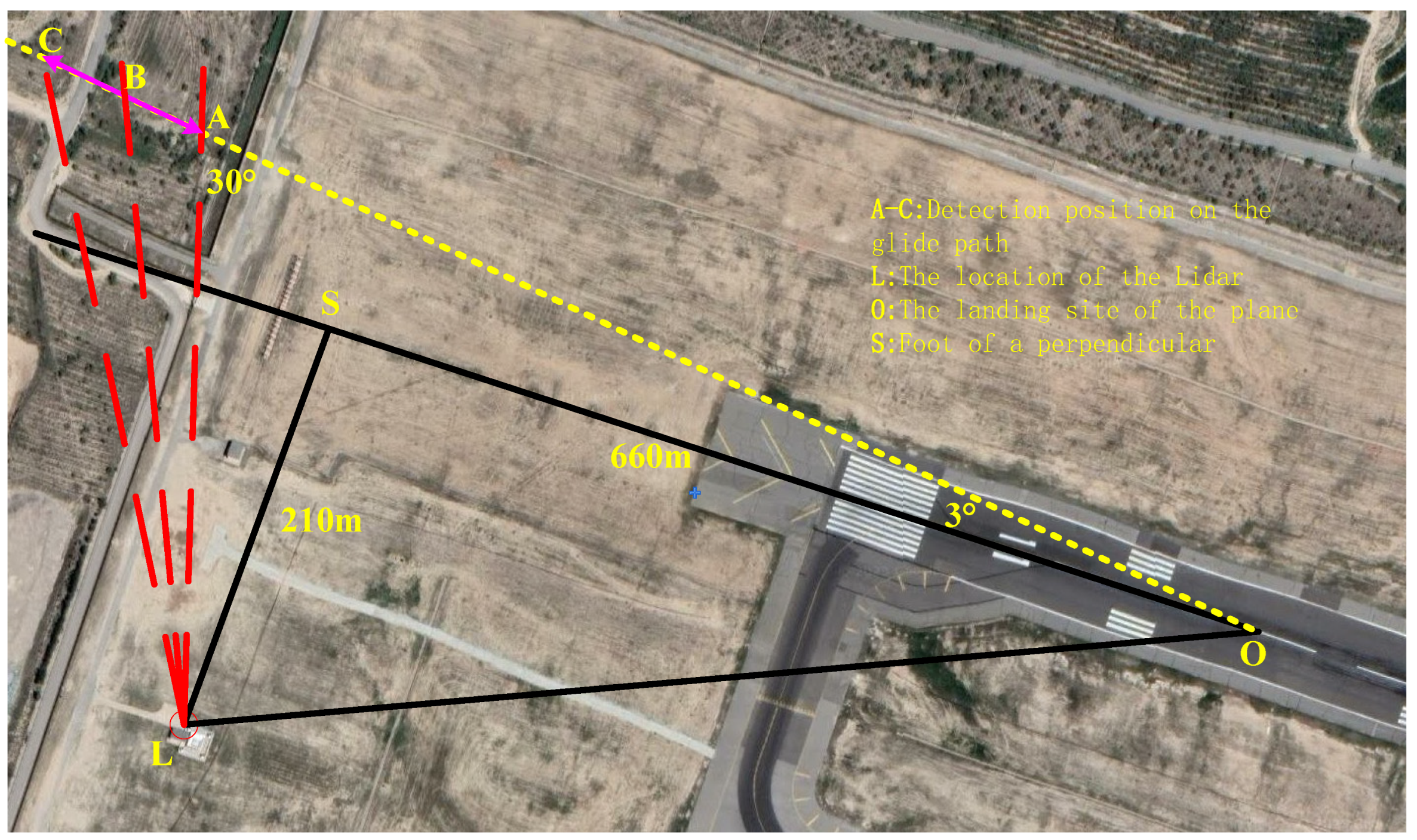
The specific data processing procedures are expounded as follows. At the outset, the headwind speed along the glide path was calculated. When the angle between the laser beam and the aircraft flight path was less than 30°, the radial wind speed nearest to the glide path position was ascertained as the glide path speed at that specific location. Moreover, individual isolated points at the distal end, which might be attributed to clouds, were excluded. Subsequently, the headwind speed of the glide path at diverse locations was obtained via interpolation at 100 m intervals (corresponding to an approximate height of 5 m at a 3° elevation) along the glide path direction, with the landing point designated as the origin. Subsequently, data quality control predicated on a 5-point median filter was carried out to smooth the interpolated data. Inasmuch as the wind field characteristically manifests pronounced gust features, and when an aircraft voice report is available, it is conventionally evaluated based on the deviation of the aircraft trajectory, which is temporally delayed. Thus, the time of the aircraft voice report was taken as the starting point, and the headwind profiles of the three previous consecutive SP scans were averaged (within a time interval of 13–20 min) to compute the current headwind wind profile.

Subsequently, the slope detection algorithm, the S-factor algorithm, and the modified F-factor algorithm were utilized to process the headwind profile and procure the wind shear intensity values at different locations and altitudes. Ultimately, the maximum values of the computed wind shear intensity were selected and employed as an alarm indicator. Moreover, all SP data from 09:00 to 19:00 on 5 April 2023 were processed to extract the maximum values for different algorithms, thereby facilitating the assessment of the validity and efficacy of these algorithms. This comprehensive data processing methodology is of utmost importance for guaranteeing the accuracy and reliability of the wind shear detection and analysis, as it takes into account diverse factors and uncertainties inherent in the wind field and data collection process. For example, the interpolation step contributes to generating a more continuous and representative headwind speed profile, while the median filter alleviates the influence of spurious data points. The averaging of the headwind profiles in accordance with the aircraft’s voice report time is designed to address the time-lagged nature of the aircraft’s trajectory-based wind shear detection and furnish a more accurate and timely evaluation of the wind shear conditions.

3.2. Wind Shear Identification Algorithm

3.2.1. The Slope Detection

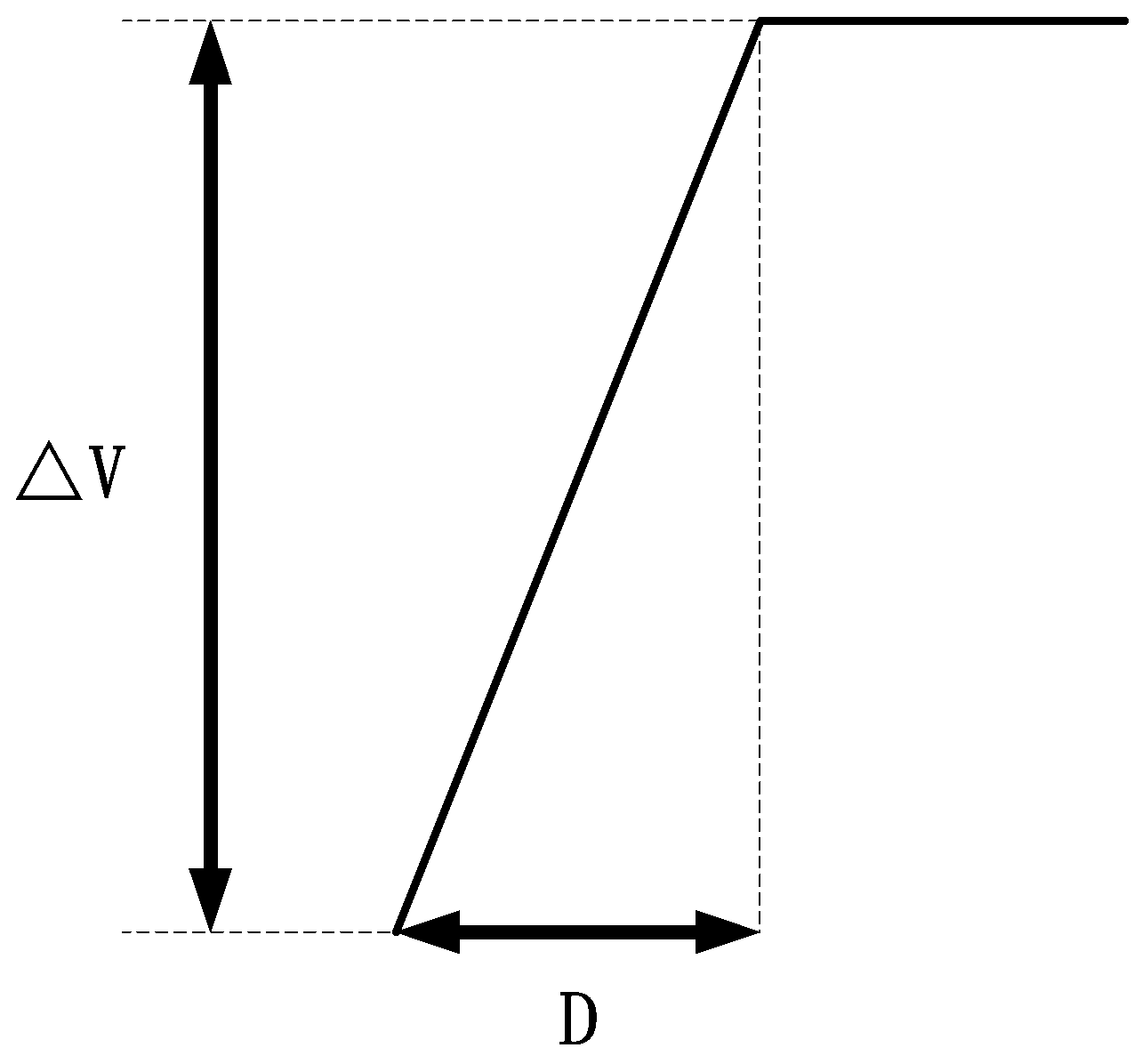
The principle of the slope detection algorithm is illustrated in Figure 5. The slope herein pertains to the aircraft’s glide path. In the figure, $D$ represents the length of the glide path over a specific distance, and V is the variation in wind speed within the length of the glide path. The slope detection algorithm is based on the definition of wind shear. The crux of this method lies in calculating the change value of wind speed on the wind profile over a certain distance and further differentiating the intensity in accordance with the change value.

Owing to the presence of certain noise data within the original wind profile data, which can exert an impact on the ultimate wind shear detection outcomes, it is essential to conduct filtering on the original wind profile prior to implementing the slope detection algorithm. A sliding average method is frequently employed. The original wind profile is denoted by $U$, and the wind profile processed via the smoothing formula is represented by $UI$. The smoothing formula is presented in Formula (1).

$$UI={\displaystyle \frac{1}{4}}U(d-\Delta d)+{\displaystyle \frac{1}{2}}U(d)+{\displaystyle \frac{1}{4}}U(d+\Delta d)$$

(1)

In Formula (1), the sampling distance is represented by $∆d$, and the Wind Data Point is represented by $d$. After smoothing the original wind profile, the slope can be detected, and the slope detection formula is shown in Formula (2).

$$UID(\tilde{d})=UI(d+D)-UI(d)$$

(2)

The $\tilde{d}$ in Formula (2), equal to $d+D/2$, represents the midpoint of the low-level wind shear, and $D$ represents the detection distance, that is, the length of the slope.

The intensity of low-level wind shear is expressed by the gradient of wind velocity change per unit distance. The International Civil Aviation Organization (ICAO) divides wind shear into four grades, mild, moderate, strong, and severe, as shown in

Table 2. Classification of wind shear by ICAO.

Grades	Effects on Flight	ICAO
		Wind Shear Within 30 m of the Atmosphere (m/s)	Intensity (1/s)
Mild	Slight change in aircraft trajectory and airspeed	<2.0	<0.067
Moderate	Greater difficulty in maneuvering the aircraft	2.0–4.0	0.068–0.138
Strong	May lead to loss of control of aircraft	4.0–6.0	0.139–0.206
Severe	Loss of maneuverability, causing serious harm	>6.0	>0.206

. In practical operation, it should be noted that the temporal and spatial resolution of the data needs to be considered, although this aspect is not directly related to the intensity grading. According to ICAO, the wind speeds corresponding to different levels of horizontal wind vertical shear are as follows. For the mild level, it is ≤2 m/s per 30 m vertical range; the moderate level ranges from 2.1 to 4.0 m/s per 30 m vertical range; the strong level is from 4.1 to 6.0 m/s per 30 m vertical range; and the severe level is greater than 6.0 m/s per 30 m vertical range. In this paper, the minimum severe wind shear strength of the ICAO standard is used as the warning threshold, because a level below it could lead to loss of control of the aircraft, and the aircraft must steer clear of them when the higher ones are encountered.

3.2.2. Shear Intensity Factor

The wind shear strength is determined by the total wind speed variation and the wind speed variation rate, so the wind shear strength factor formula is the product of these two terms, which is defined as

$$S=({\displaystyle \frac{dV}{dt}}){({\displaystyle \frac{\Delta V}{V_a}})}^2={\left({\displaystyle \frac{\Delta V}{R^{1/3}}}\right)}^3{V_a}^{-1}$$

(3)

where $dV/dt$ is the rate of change in wind speed, $∆V$ is the magnitude of the change in wind speed, R is the corresponding length of detection, and $V_a$ is the approach speed of the aircraft during landing. $∆V/V_a$ is the total change in wind speed, which usually affects the aircraft more than the rate of change in wind speed; this is also the reason why the traditional slope algorithm only detects the change of wind speed for wind shear warning, so the term is quadratic.

In this paper, the slope length is 600 m (30 m height; the 3° elevation corresponding to height is 573 m, according to 600 m), and the S-factor intensity partition range corresponding to different strength grades can be calculated, so the minimum severe wind shear strength, 0.711, is used as the warning threshold.

3.2.3. Modified F-Factor

The force of the airplane in the wind field mainly includes the thrust $T$ of the airplane engine, the resistance $D$ of the air to the airplane, and the gravity $W$ of the airplane itself. In a uniform wind field, the total energy of the aircraft per unit gravity can be expressed by Formula (4).

$$E=H+{\displaystyle \frac{V_a}{g}}{V}_a=V_a[{\displaystyle \frac{(T-D)}{W}}-F]$$

(4)

where $H$ is the altitude of the aircraft, $V_a$ is the airspeed of the aircraft, and g is the gravitational acceleration. Then, the F-factor can be expressed as

$$F={\displaystyle \frac{U_X}{g}}-{\displaystyle \frac{U_h}{V_a}}={\displaystyle \frac{V_a}{g}}{\displaystyle \frac{d{U}_x}{dR}}-{\displaystyle \frac{U_h}{V_a}}$$

(5)

The modified F-factor algorithm is proposed by the Civil Aviation University of China after discovering the relationship between the wind speed on the glide slope, $U_x$, and the vertical wind, $U_h$, through modeling, as shown in (6):

$$F_m={\displaystyle \frac{V_a}{g}}\left(1-{\displaystyle \frac{\lambda gH}{{V_a}^2}}\right){\displaystyle \frac{d{U}_x}{dR}}$$

(6)

where $R$ is the distance between two points on the glide slope. At present, there is no clear definition of the alarm threshold of the F-factor algorithm in the world. The F-factor warning threshold, ±0.105, proposed by Hinton in 1993 is used in this paper [24]. When the F-factor exceeds the threshold, it is considered a danger to the aircraft.

4. Weather Process

4.1. Weather Map

On 5 April 2023, Beijing time (it should be noted that all times in this paper refer to Beijing time), a wind shear event was triggered by a frontal system at Xining International Airport, China. This incident resulted in the grounding of multiple flights. The meteorological conditions were manifested as cloudy skies, with light snow evolving into thin clouds, accompanied by the transformation from high-blowing sand to low-blowing sand. Easterly winds prevailed, exhibiting an average speed in the range of 5 to 13 m per second. The 500 hpa weather map (illustrated in Figure 6) at 08:00 on the same day indicated that Xining Airport was under the influence of the southwest airflow in the pre-trough area. The location was positioned at the leading edge of a rapid flow zone. After a period of 12 h, the high-altitude trough underwent a transition, accompanied by a prominent rapid flow axis overhead. This area was converted into a frontal zone due to the movement of the high-altitude trough and was gradually affected by the rear part, which was situated within the cold and warm advection convergence area. Significantly, an obvious convergence area was observable under the domination of cold advection and with a temperature dew point difference of less than 5 °C, making the area humid. On the ground map, at 08:00, the airport was under the control of the rear part of a cold front, presenting dense, cold, high-pressure isobars. An apparent wind field convergence area was visible in the northern and frontal parts of the airport, which is favorable for changes in wind direction. Additionally, the cold air exhibited a backflow after the cold front, leading to a backflow of easterly winds and a partial invasion of cold air from the east. The synoptic-scale weather patterns and their evolutionary processes are of essential importance in comprehending the origin and development of wind shear events. The interaction between the upper-level trough and the surface cold front, in conjunction with the associated advection and convergence mechanisms, can result in substantial alterations in the wind field and the thermodynamic structure. The existence of cold advection and the convergence zone can trigger vertical motions and changes in wind speed and direction, thereby enhancing the probability of wind shear formation.

The ground weather map at 11:00 on that particular day (depicted in Figure 7) discloses a remarkable pattern of dense isobars and substantial pressure gradient forces in the western and northern sectors of Xining Airport. This implies the intrusion of cold air masses from the west and northwest directions into the domain of study. At 14:00, 17:00, and 20:00, the consecutive ground weather maps illustrated that Xining Airport was gradually being dominated by the cold air emanating from the west and northwest. By 20:00, the 500 hpa high-altitude map manifested the displacement of the high-altitude trough away from the airport. This temporal progression of weather systems, as illustrated by the ground and high-altitude weather maps, is of essential significance in comprehending the meteorological backdrop and its prospective ramifications for wind shear events. The movement and interaction of diverse air masses, as manifested by the alterations in isobar patterns and the position of the high-altitude trough, can exert a profound influence on the wind field attributes. The incursion of cold air from particular directions can precipitate rapid modifications in wind speed and direction, thereby augmenting the probability of wind shear formation. A comprehensive analysis of such weather map sequences can furnish valuable perspectives for the prediction and alleviation of wind shear hazards, especially within the domain of aviation safety.

4.2. Aircraft Voice Reports

Aircraft voice reports assume a critical function within the domain of civil aviation [25]. They are directly conveyed by pilots when civil aircraft experience hazardous meteorological conditions, including turbulence, ice accretion, or wind shear during flight. These reports constitute a valuable adjunct to the extant array of civil aviation weather observation instruments and are of cardinal significance in determining the actual occurrence of wind shear events. In circumstances where the accurate true values of wind shear are lacking, aircraft voice reports can ordinarily be utilized as reference true values, thus proffering essential data for further scrutiny and investigation.

On 5 April 2023, within the time interval from 15:18 to 17:05, the airport under consideration received a cumulative total of 8 aircraft voice reports. This instigated substantial operational modifications, wherein 3 flights recommenced their intended trajectories subsequent to suitable appraisals and 5 flights elected to land at substitute airports, as expounded in

Table 3. Aircraft voice reports at the airport on 5 April 2023.

Time	Causes	Results	Locations	Within Lidar Range or Not
15:11	Wind direction and speed excessive variation	Resumption of flight	Runway 11 at 2 km, height 200–300 m	Yes
15:29	Wind shear intensity unknown	Standby for landing	Height 4800 m	No
15:31	Wind shear intensity unknown	Resumption of flight	Before grounding on runway 11, height 12.19 m	Yes
15:32	Wind shear intensity unknown	Standby for landing	Height 4800 m	No
15:47	Wind shear intensity unknown	Standby for landing	Height 4800 m	No
16:05	Experiencing top wind	Resumption of flight	Runway 11 entrance, 5 km Height 15.24 m	Yes
16:06	Wind direction and speed sudden changes	Standby for landing	Height 4800 m; sudden change in wind direction and speed	No
16:40	Weather	Standby for landing	Height 6300 m	No

. Among these reports, in 7 instances, it was distinctly manifested that the alteration in flight plan was directly ascribable to the incidence of wind shear. The last report received was at 16:40. Based on the analysis of the weather map in Section 4.1, the airport wind field started from the east wind at 8:00 and then experienced the invasion of west and northwest winds, gradually being controlled by them. This indicates a strong correlation between wind shear occurring during the passage of cold air. It is worthy of note that the Lidar system installed at the airport exhibited a detection range of less than 10 km. This corresponded to a glide path scan altitude of below 500 m. In light of this constraint, the three voice reports that resided within the Lidar’s detection purview, namely those generated at 15:11, 15:31, and 16:05, were chosen as the principal focus of this research. The residual reports, notwithstanding their position outside of the Lidar’s range, still retained value and could be employed as valuable references, facilitating a more comprehensive understanding of the overall wind shear scenario and its effects on flight operations. The selection of these specific reports within the scope of Lidar is based on the principle of utilizing data directly related to Lidar measurements. By focusing on these reports, a more detailed analysis of wind shear characteristics within detectable areas can be conducted, which can help us understand the processes of wind shear occurrence, movement, etc. This is essential for improving aviation safety and simplifying flight operations under different meteorological conditions.

5. Results

The three algorithms were utilized to calculate the wind shear intensity by leveraging the Lidar data procured from the SP scanning mode. The headwind speed constituted the foundation for computing wind shear information, and the incidence of wind shear was determined in compliance with the pre-defined thresholds. As illustrated in

Table 4. Intensity levels and thresholds of different algorithms.

Grades	Effects on Flight	Slope Detection Thresholds (1/s)	S-Factor Threshold ( ${\mathbf{m}}^{2/3}{\mathbf{s}}^{-1}$)	Modified F-Factor Threshold
Mild	Slight change in aircraft trajectory and airspeed	≤0.067	0–0.237	−0.105–+0.105
Moderate	Greater difficulty in maneuvering the aircraft	0.068–0.138	0.237–0.474
Strong	May lead to loss of control of aircraft	0.139–0.206	0.474–0.711
Severe	Loss of maneuverability, causing serious harm	>0.206	>0.711	<−0.105 or >+0.105

, the threshold value for the slope detection and S-factor were ascertained by referring to the wind shear rating criteria stipulated by ICAO, which classifies the wind shear rating into four disparate groups. The minimum severe wind shear strength of the standard set by ICAO is used as the warning threshold, as described in Section 3.2.1. Regarding the F-factor, in light of the lack of an international standardized warning threshold, empirical thresholds are prevalently employed in practical applications. Chan et al. employed aircraft voice reports as the wind shear reference values and experimentally ascertained that the negative F-factor exhibits superior performance in wind shear warnings in contrast to the positive F-factor. Additionally, the warning threshold applicable to the flight operations at Hong Kong International Airport was −0.05. In this study, the F-factor warning threshold proposed by Hinton in 1993 was chosen. It is deemed that exceeding this F-factor value presents a hazard, notwithstanding the absence of further classification. The congruence of the results of different algorithms was appraised by comparing the severity levels of the slope detection and the S-factor with the warning outcomes of the modified F-factor. This comprehensive evaluation methodology is of primordial importance for validating the dependability and precision of the different algorithms in detecting and appraising wind shear, as it accommodates the variegated characteristics and limitations of each algorithm. The calibration of the S-factor threshold and the selection of the F-factor threshold were effected to optimize the performance of the algorithms and ensure more accurate identification and quantification of wind shear events, which is of cardinal significance for augmenting aviation safety and furnishing more precise meteorological support for flight operations.

5.1. General Analysis of Local Winds

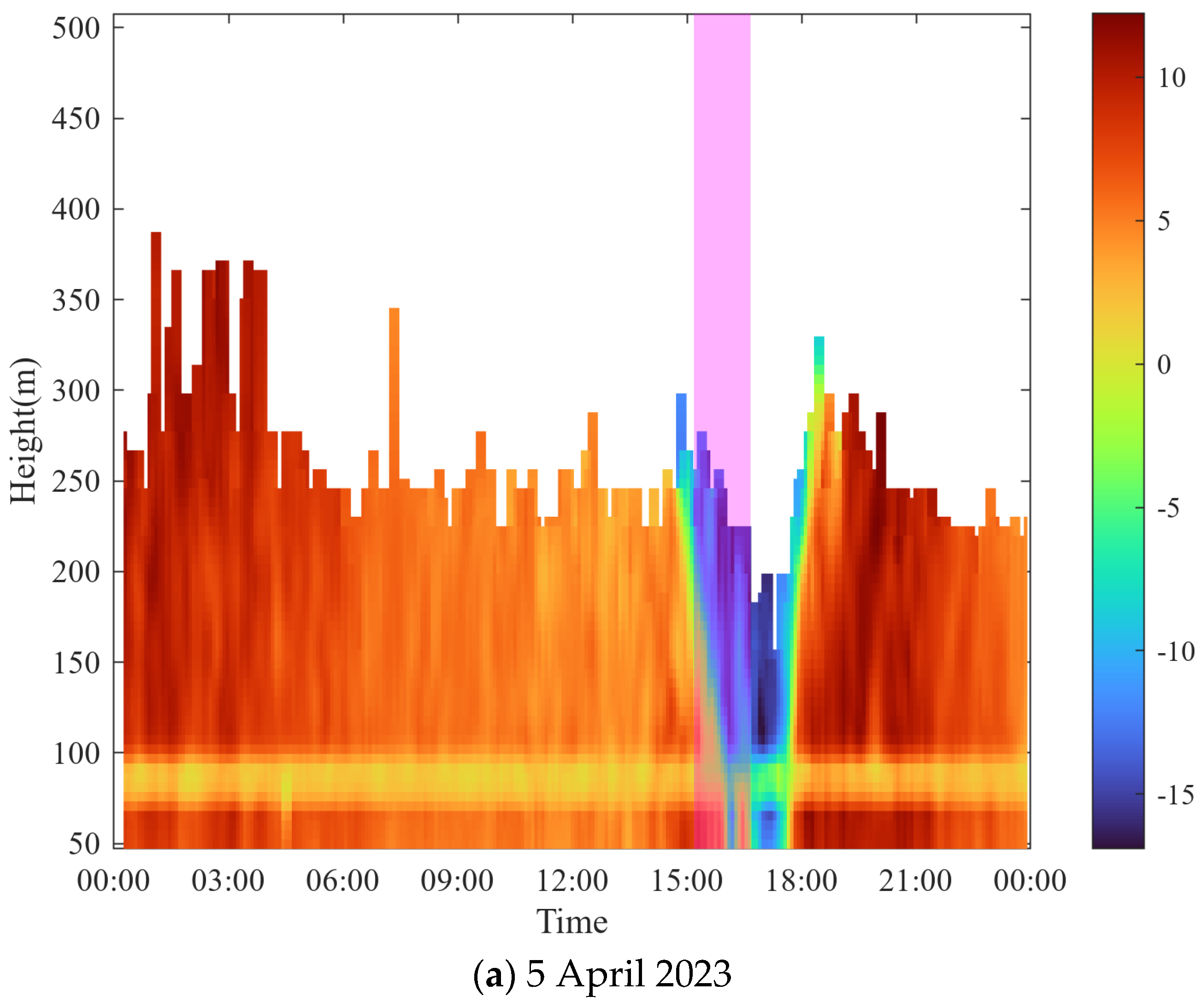
The flight arrival times during the day were within the range of 07:36 to 22:50, and all SP scans within the time interval from 09:00 to 19:00 were subjected to analysis. As illustrated in Figure 8a, a conspicuous wind speed discontinuity layer was detected at altitudes ranging from 70 to 100 m over an extended period. This was potentially attributable to the existence of an inversion temperature at this altitude. From high to low altitudes, there is a progression from a downwind condition to an upwind condition. After the wind shear has elapsed, it returns to an upwind state. The wind shear event transpired at an altitude of 250 m from 14:42 to 18:13, with a duration of approximately 3.5 h (211 min). The first half of the wind shear event substantially corresponded with the aircraft flight reports (light purple shaded area in the figures), whereas no aircraft flight reports were transmitted in the second half.

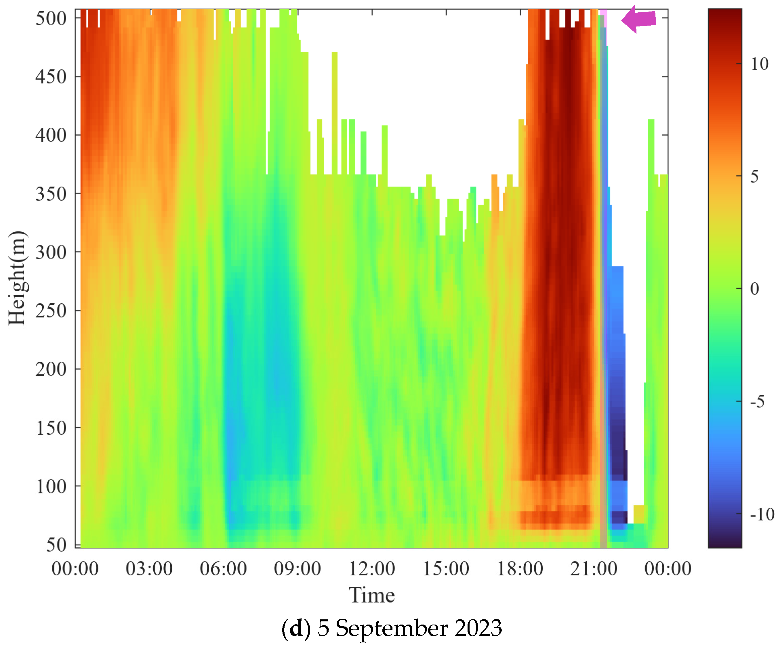
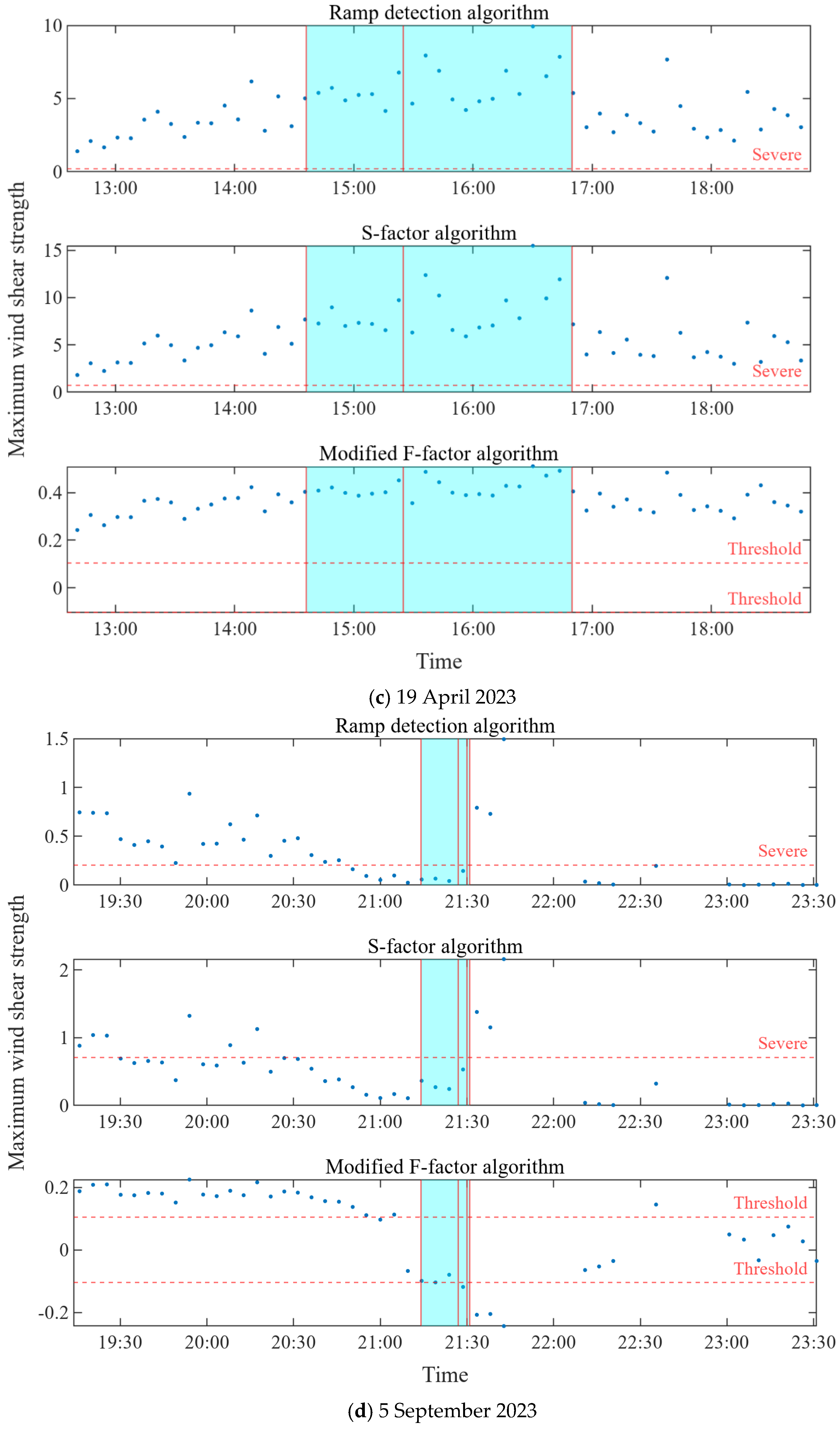
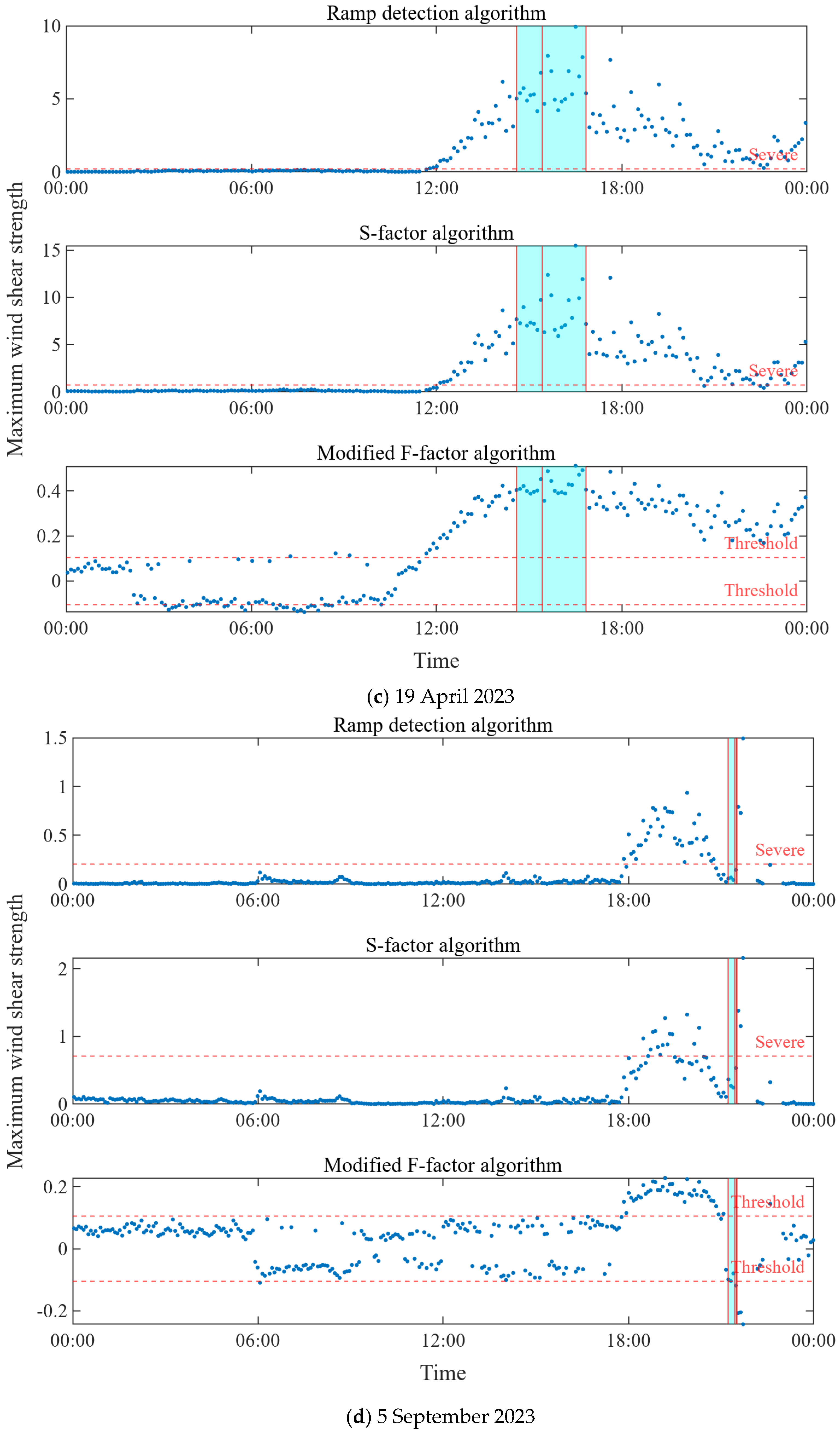
Similarly, this study processed headwind profile variations for three additional cases, as depicted in Figure 8. On 10 April 2023, the vocal reports occurred prior to a sudden change in wind direction, whereas on 19 April 2023, they happened after such a change. In the case of 5 September 2023, the reports coincided with the wind direction shift. Analysis of the vocal reports, combined with the findings, suggests two reasons for these occurrences. First, the wind field is mobile; wind shear can enter and exit the detection range (this point is preliminarily confirmed in Figure 8). Second, the location of the vocal reports does not necessarily fall within the detection range or even in the vicinity of the airport.

5.2. Headwinds from Different Algorithms

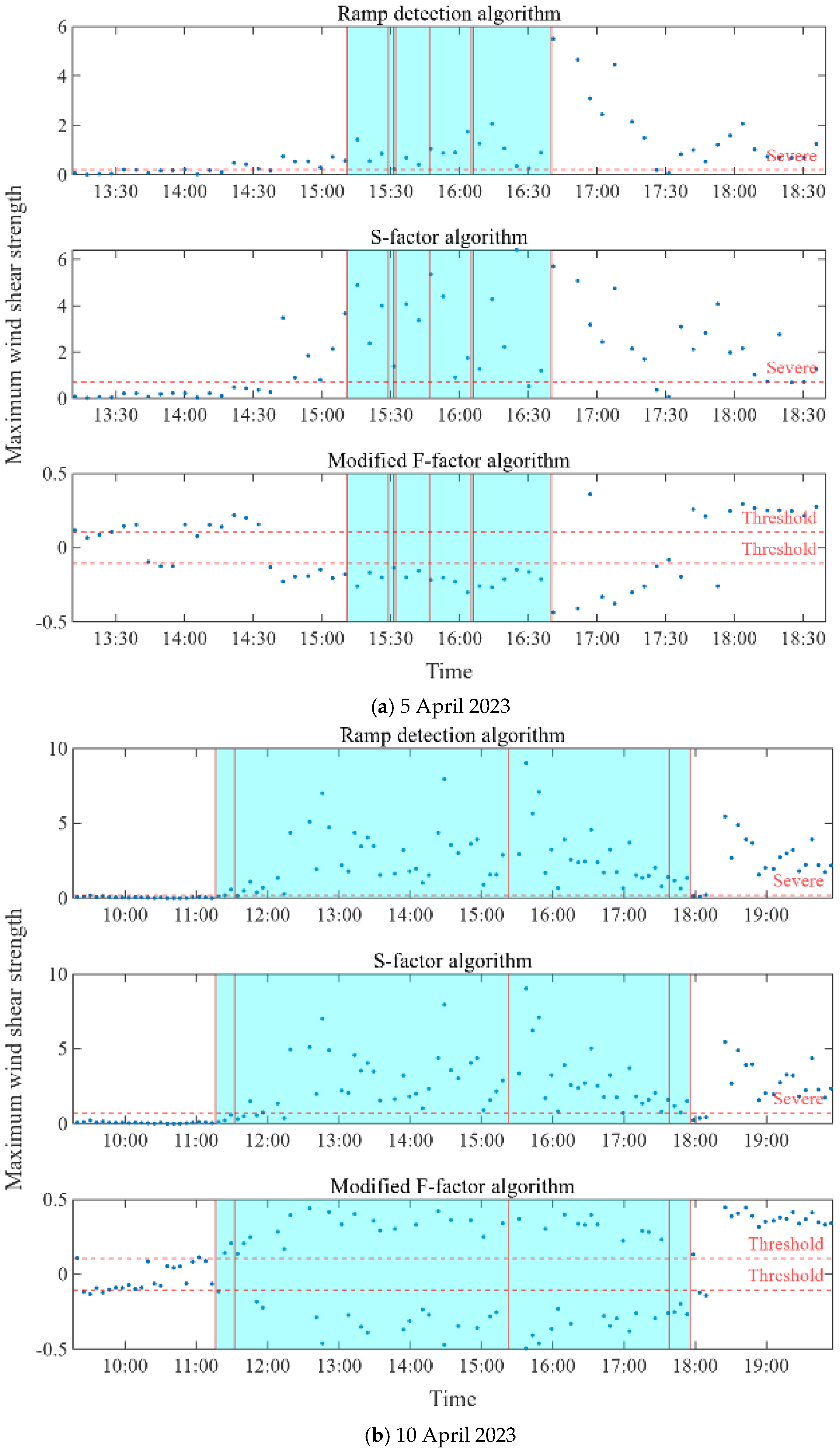
The headwind profile was comprehensively analyzed through the utilization of the three wind shear recognition algorithms, as illustrated in Figure 9, and the blue-shaded segment represents the aircraft voice reports. In Figure 9a, before 14:00, it was ascertained that the shear values computed by both the single slope algorithm and the S-factor algorithm principally resided below the predefined severity level. Concurrently, the values of the modified F-factor were mainly located in the positive direction and exceeded the established threshold. Significantly, when the aircraft voice reports were transmitted, the maximum shear values obtained from both the single slope algorithm and the S-factor algorithm surpassed the threshold, and these values were substantially higher than the maximum shear values documented in the preceding period. The performance in the other three cases is also similar. In contrast, within the same time interval, the modified F-factor was predominantly in the negative direction and exceeded the threshold. This discovery was in consonance with the experimental outcomes procured by P.W Chan, thereby further corroborating that the negative F-factor demonstrates enhanced performance in wind shear alerts in comparison to the positive F-factor. However, we observed that the aforementioned situation was not as evident in the case of 5 September 2023. By examining the algorithm detection results for the case on that day, as depicted in Figure 10, the times of the reports for cases (a), (b), and (c) all fall within the periods when the detection results of the three algorithms exceeded the threshold, while case (d) occurred afterward. Nevertheless, both the vocal reports and the detection algorithms confirmed the presence of wind shear.

It was discerned that for a considerable period following the issuance of the aircraft voice report alert, the results produced by the three algorithms did not experience significant alterations. The potential cause for the lack of wind-shear-related aircraft voice reports during this phase could plausibly be ascribed to the modification of the landing runway, specifically, the employment of runway 29 for landing. This alteration of the landing runway might have instigated diverse wind conditions and interactions, which subsequently influenced the occurrence and reporting of wind shear events. A meticulous exploration of such factors and their ramifications is essential for a more in-depth comprehension of the nexus between wind shear detection algorithms, actual wind shear manifestations, and the corresponding reporting procedures in the context of aviation safety.

5.3. Wind Shear Strength from Different Algorithms

In consideration of the gusty characteristic of the wind, a sliding average of the three adjacent instantaneous winds was employed to compute the head-on wind profile of the glide path. Figure 8 illustrates the variation of the maximum shear values over the time interval. The maximum shear values for both the slope detection algorithm and the S-factor algorithm were within the severe range, and the maximum shear values for the modified F-factor algorithm were within the negative threshold range. A slight variation was discerned in the results, and the three algorithms exhibited a high degree of consistency. Based on the outcomes of the analysis in Figure 8, Figure 9 and Figure 10, the results generated by the three algorithms can be utilized to assess the occurrence of wind shear with a high level of reliability.

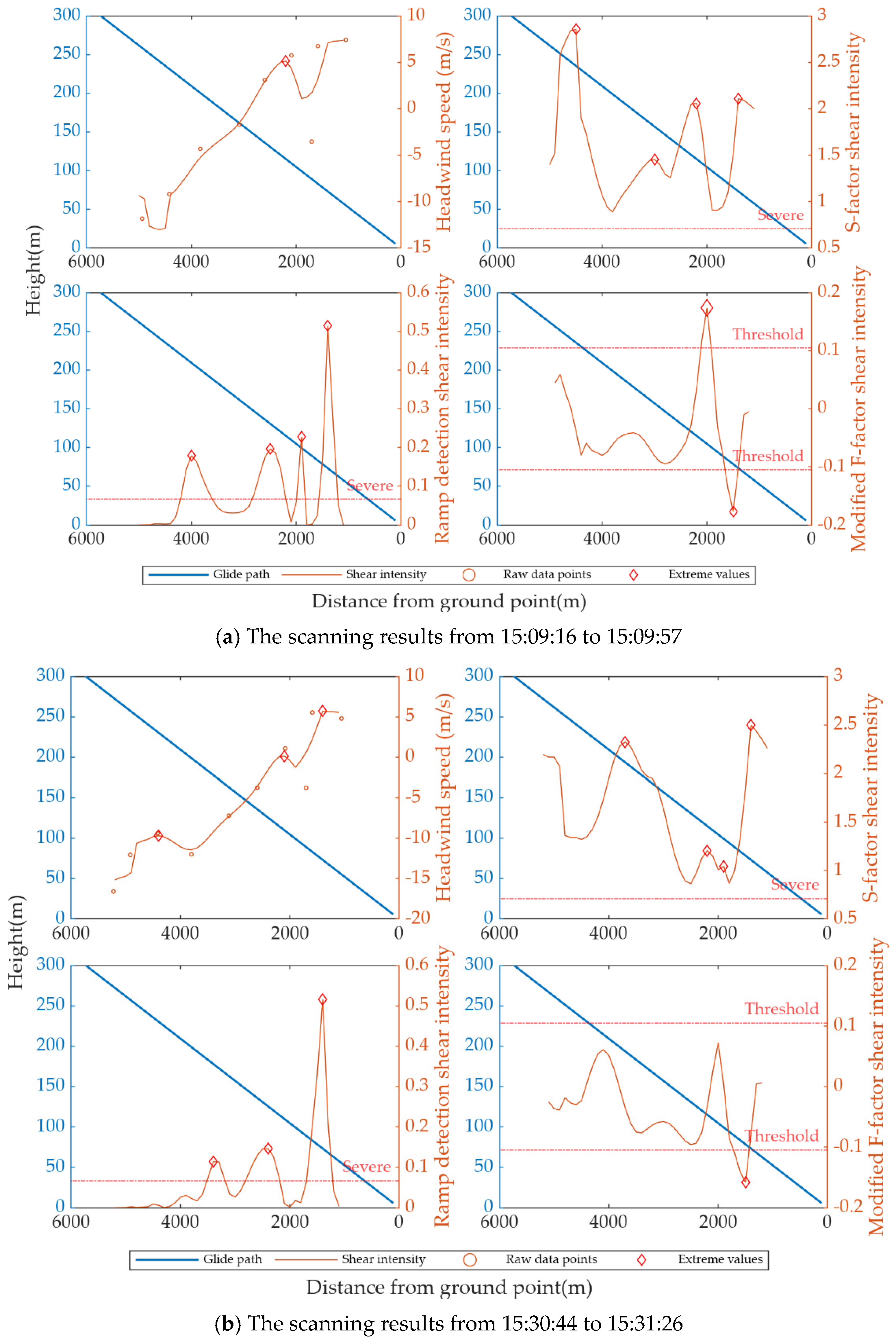
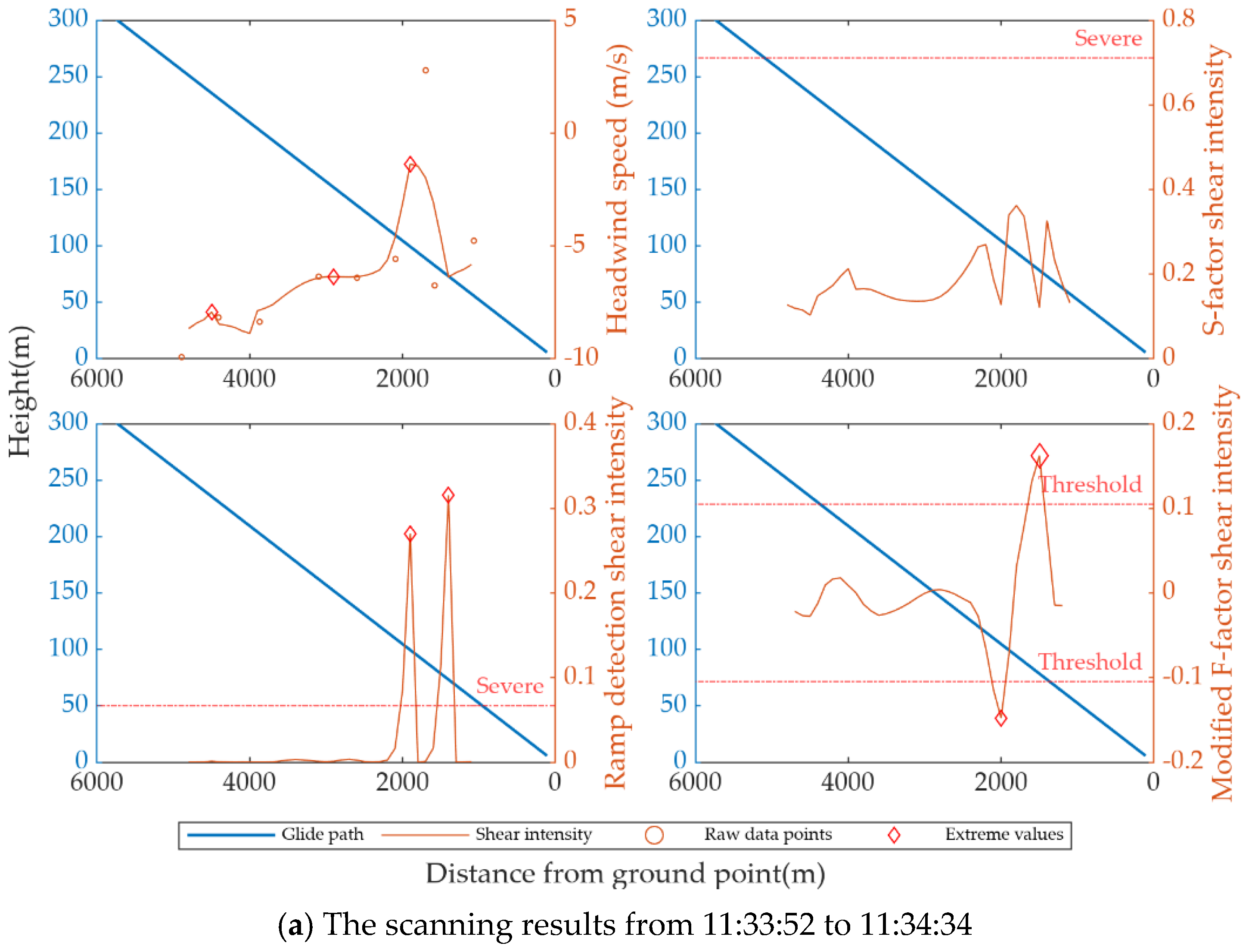
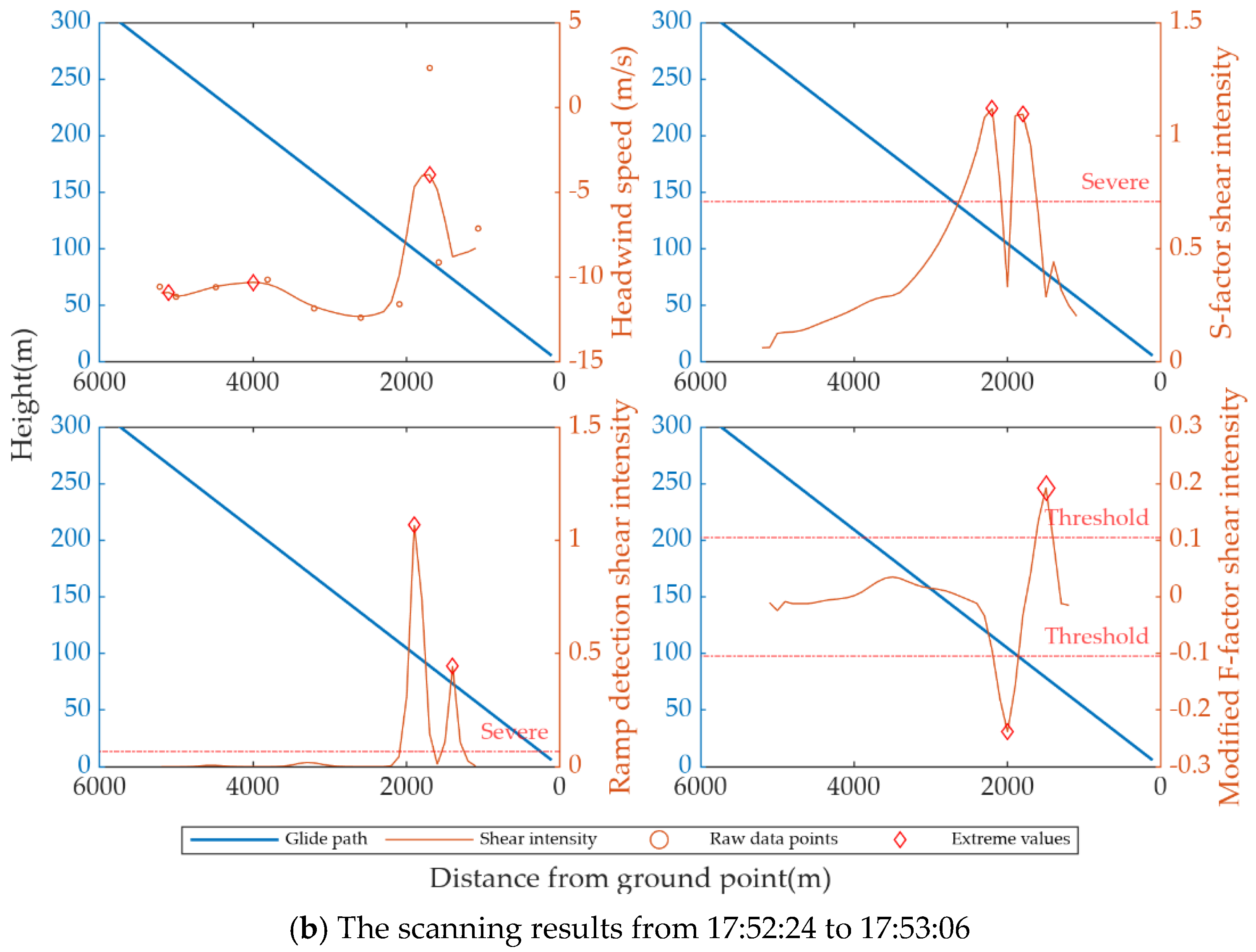
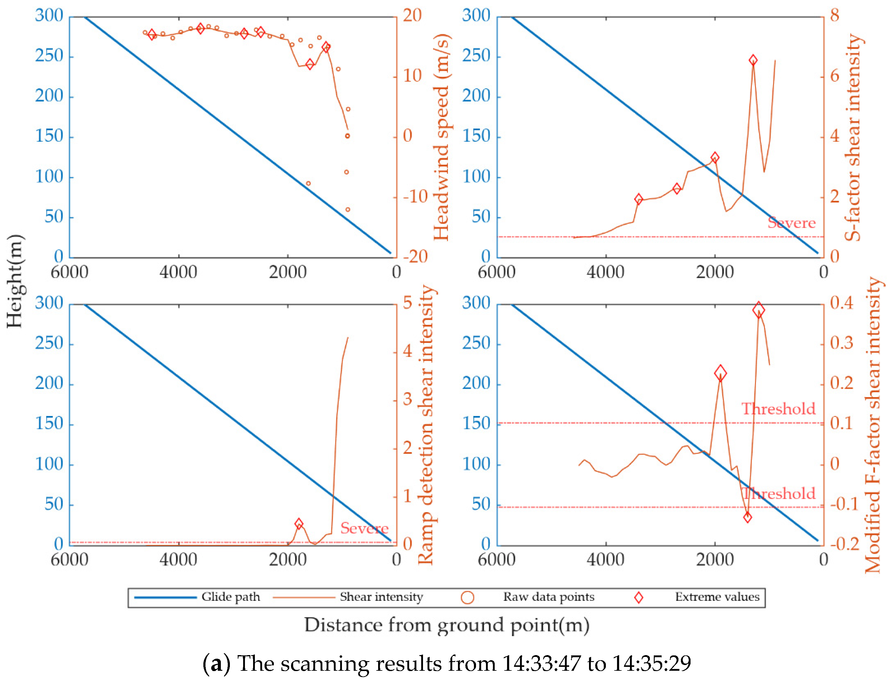
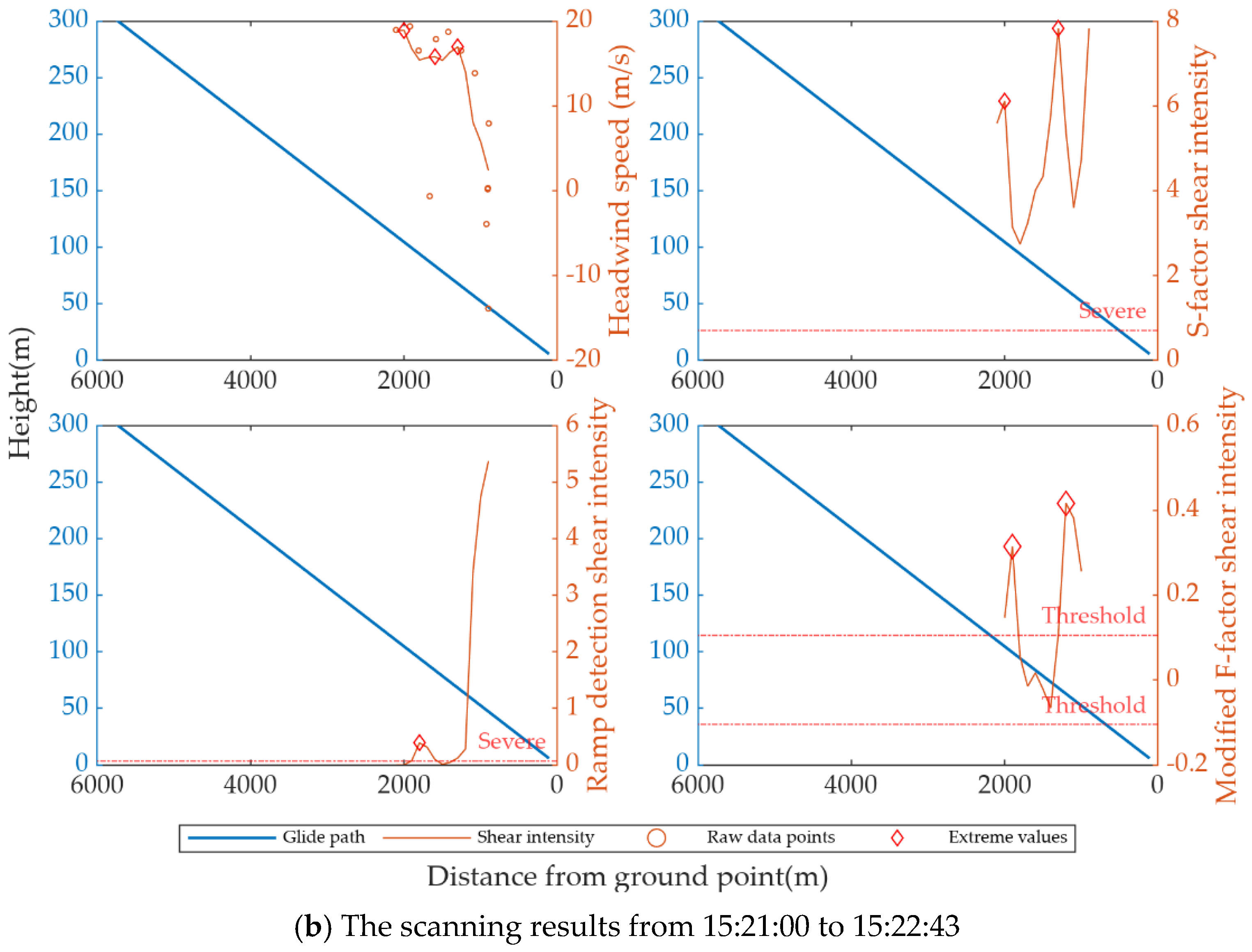
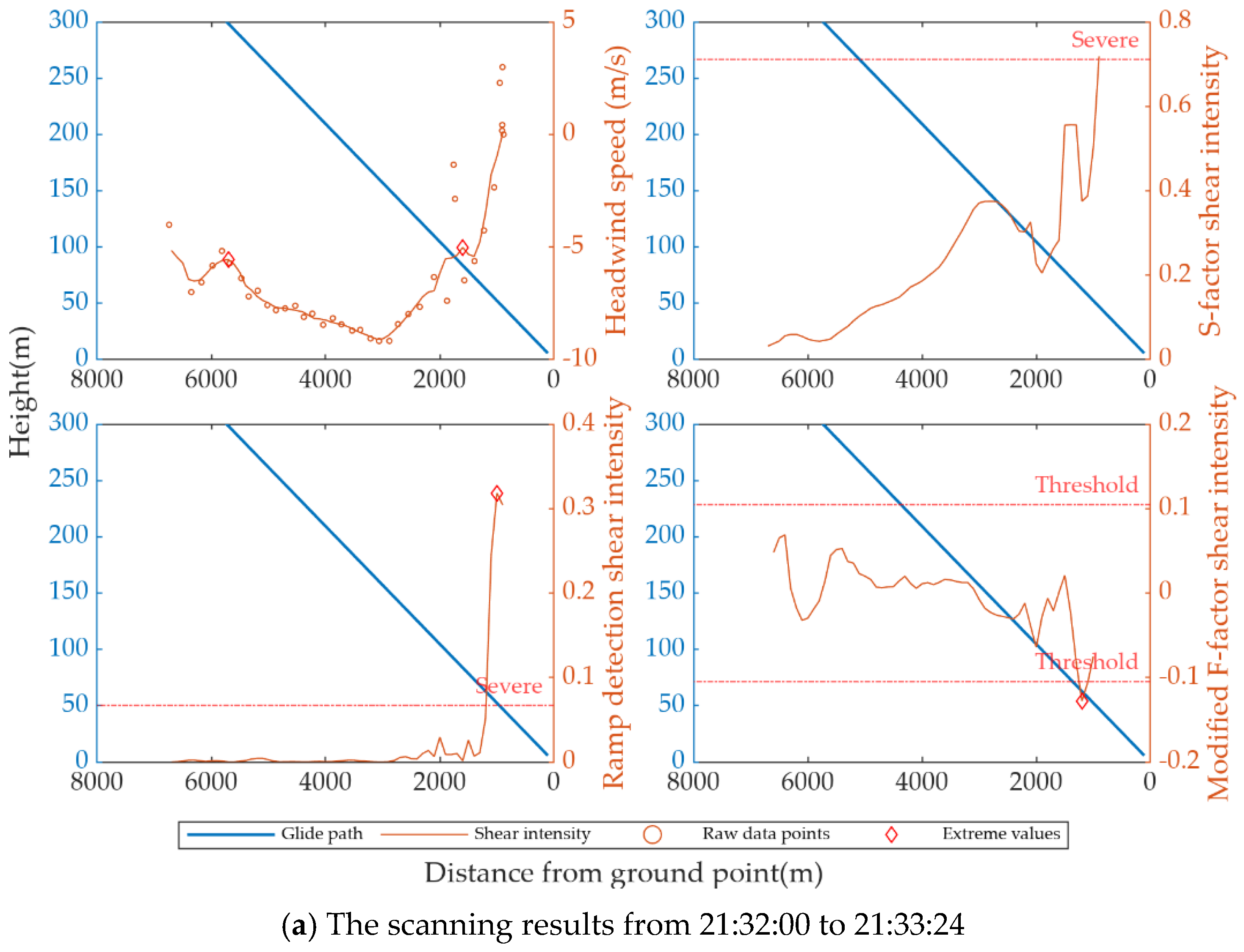
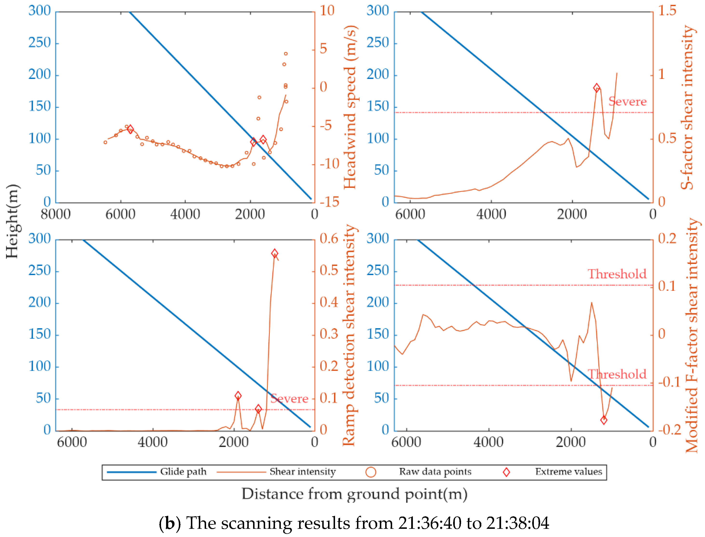
The three instances of wind shear, which were communicated via aircraft voice reports within the Lidar measurement range, were subjected to further analysis with the aim of clarifying the relationship between the head-on wind speed and the variation in the shear values yielded by each algorithm at diverse locations along the slope. In accordance with the data processing procedure detailed in Section 3.1, the SP scan observations that were closest to the time when the aircraft voice report was issued were chosen for analysis. These observations were all conducted within 5 min of the voice report, as depicted in Figure 11, Figure 12, Figure 13 and Figure 14. The three wind shear algorithms were employed to conduct further analyses. Regional extreme points are denoted in each figure with the intention of facilitating a comparison of the results obtained from different algorithms, as illustrated in Figure 11, Figure 12, Figure 13 and Figure 14.

(1)

When comparing the headwind profile of the glide path along the aircraft landing direction (ranging from high to low altitude), it was observed that the wind gradually transitioned from a downwind state to an upwind state. In these results, more than two algorithms consistently detected values exceeding the prescribed thresholds, thereby validating the effectiveness of considering the detection results from these algorithms as a basis for issuing alerts.

(2)

The three wind shear algorithms did not exhibit complete consistency, as deviations were manifested in the locations of the extreme values. Consequently, the application of a single algorithm might lead to insufficient accuracy in detecting wind shear. Given that the atmosphere possesses a certain degree of continuity, a comprehensive assessment should be made based on the observation results to enhance the accuracy.

6. Conclusions

In this present study, an in-depth and comprehensive exploration was carried out regarding the low-level wind shear process instigated by frontal passage. Through the utilization of the headwind profile data of the glide path, which were obtained from the SP scanning mode, and the application of three wind shear recognition algorithms, with the aircraft voice reports being adopted as the reference true values, the effectiveness of the three algorithms is verified.

Firstly, the comparison between the results generated by the three algorithms and the aircraft voice reports substantiated the feasibility of these algorithms in detecting wind shear events that might potentially affect aircraft. This multi-algorithm strategy offers a more reliable and sturdier framework for wind shear identification, facilitating a more exhaustive and comprehensive evaluation from diverse algorithmic viewpoints. Secondly, it was ascertained through the utilization of the three disparate algorithms that wind shear events could assuredly be detected, notwithstanding the fact that the results procured from these algorithms were not completely congruent. Such variations underscore the intricacy and variability that are intrinsically associated with wind shear detection, thereby accentuating the necessity of comprehensive understanding and integration of multiple algorithmic outcomes. Furthermore, a significant characteristic of wind shear, namely, its persistence, was disclosed. As manifested by the scanning outcomes, wind shear events were determined to persist within the scanning range for a particular duration, either as spatial translocation or temporary vanishing in the temporal realm. This revelation augments our comprehension of the dynamic essence of wind shear and bears consequences for its precise surveillance and prognostication.

Nevertheless, it ought to be noted that the present study was circumscribed to a solitary sample of wind shear events within the context of frontal passage. Future research initiatives will be centered around incorporating a more extensive array of cases, amalgamating the detection capabilities of multiple scanning modalities, and augmenting wind shear prediction. It is anticipated that the combined outcomes of the three algorithms can function as a more advantageous and dependable criterion for wind shear warning. Weighting the alarm results of multiple algorithms as the basis for warning would be a good strategy, but further experimentation is needed to determine the effectiveness. In total, this study not only amplifies our understanding of wind shear processes but also establishes a bedrock for further research and practical applications in alleviating the risks correlated with wind shear within the context of aviation.

References

1. Li, L.; Shao, A.; Zhang, K.; Ding, N.; Chan, P.-W. Low-Level Wind Shear Characteristics and Lidar-Based Alerting at Lanzhou Zhongchuan International Airport, China. J. Meteorol. Res. 2020, 34, 633–645. [Google Scholar] [CrossRef]
2. Huang, J.; Ng, M.K.P.; Chan, P.W. Wind Shear Prediction from Light Detection and Ranging Data Using Machine Learning Methods. Atmosphere 2021, 12, 644. [Google Scholar] [CrossRef]
3. Wu, T.-C.; Hon, K. Application of Spectral Decomposition of LIDAR-Based Headwind Profiles in Windshear Detection at the Hong Kong International Airport. Meteorol. Z. 2017, 27, 33–42. [Google Scholar] [CrossRef]
4. Evans, J.; Turnbull, D. Development of an Automated Windshear Detection System Using Doppler Weather Radar. Proc. IEEE 1989, 77, 1661–1673. [Google Scholar] [CrossRef]
5. Proctor, F.H.; Hinton, D.A.; Bowles, R.L. A Windshear Hazard Index. In Proceedings of the Aviation, Range and Aerospace Meteorology, Orlando, FL, USA, 11–15 September 2000. [Google Scholar]
6. Chan, P.W. A Tail Strike Event of an Aircraft Due to Terrain-Induced Wind Shear at the Hong Kong International Airport: Tail Strike Event of Aircraft. Met. Apps 2014, 21, 504–511. [Google Scholar] [CrossRef]
7. Li, M.; Xu, J.; Xiong, X.; Ma, Y.; Zhao, Y. A Novel Ramp Method Based on Improved Smoothing Algorithm and Second Recognition for Windshear Detection Using LIDAR. Curr. Opt. Photonics 2018, 2, 7–14. [Google Scholar] [CrossRef]
8. Xia, H.; Chen, Y.; Yuan, J.; Su, L.; Yuan, Z.; Huang, S.; Zhao, D. Windshear Detection in Rain Using a 30 Km Radius Coherent Doppler Wind Lidar at Mega Airport in Plateau. Remote Sens. 2024, 16, 924. [Google Scholar] [CrossRef]
9. Weber, M.E.; Stone, M.L. Low Altitude Wind Shear Detection Using Airport Surveillance Radars. IEEE Aerosp. Electron. Syst. Mag. 1995, 10, 3–9. [Google Scholar] [CrossRef]
10. Tse, S.M.; Hagio, M.; Maeda, Y. Windshear Detection by Terminal Doppler Weather Radar during Tropical Cyclone Mujigae in 2015. Meteorol. Appl. 2019, 26, 620–631. [Google Scholar] [CrossRef]
11. Xu, T.; Ma, X.; Li, Q.; Lu, Y. Application of Low-Altitude Wind Shear Recognition Algorithm and Laser Wind Radar in Aviation Meteorological Services. Open Phys. 2023, 21, 20230154. [Google Scholar] [CrossRef]
12. Denisenkov, D.A.; Zhukov, V.Y.; Shchukin, G.G. Wind Shear Detection from Weather Radar Data. Russ. Meteorol. Hydrol. 2019, 44, 782–789. [Google Scholar] [CrossRef]
13. Ma, Y.; Li, S.; Lu, W. Recognition of Partial Scanning Low-Level Wind Shear Based on Support Vector Machine. Adv. Mech. Eng. 2018, 10, 1687814017754151. [Google Scholar] [CrossRef]
14. Zhang, J.; Chan, P.W.; Ng, M.K. LiDAR-Based Windshear Detection via Statistical Features. Adv. Meteorol. 2022, 2022, 3039797. [Google Scholar] [CrossRef]
15. Hinton, D.A. Airborne Derivation of Microburst Alerts from Ground-Based Terminal Doppler Weather Radar Information—A Flight Evaluation. In NASA Technical Memorandum 108990; NASA: Washington, DC, USA, 1993. [Google Scholar]
16. Chan, P.W.; Hon, K.K.; Shin, D.K. Combined Use of Headwind Ramps and Gradients Based on LIDAR Data in the Alerting of Low-Level Windshear/Turbulence. Meteorol. Z. 2011, 20, 661–670. [Google Scholar] [CrossRef] [PubMed]
17. Lee, Y.F.; Chan, P.W. LIDAR-based F-factor for Wind Shear Alerting: Different Smoothing Algorithms and Application to Departing Flights. Meteorol. Appl. 2014, 21, 86–93. [Google Scholar] [CrossRef]
18. Hon, K.K.; Chan, P.W.; Chiu, Y.Y.; Tang, W. Application of Short-Range LIDAR in Early Alerting for Low-Level Windshear and Turbulence at Hong Kong International Airport. Adv. Meteorol. 2014, 2014, 162748. [Google Scholar] [CrossRef]
19. Hon, K.K.; Chan, P.W. Improving Lidar Windshear Detection Efficiency by Removal of “Gentle Ramps”. Atmosphere 2021, 12, 1539. [Google Scholar] [CrossRef]
20. Wang, G.; Xu, H.; Pei, B.; Xue, Y.; Duan, X. Risk Topology Construction Method of Flight Manipulation in Turbulent-Windshear Conditions Based on Multivariate Copula Theory. IEEE Access 2020, 8, 127801–127817. [Google Scholar] [CrossRef]
21. Yuan, J.; Su, L.; Xia, H.; Li, Y.; Zhang, M.; Zhen, G.; Li, J. Microburst, Windshear, Gust Front, and Vortex Detection in Mega Airport Using a Single Coherent Doppler Wind Lidar. Remote Sens. 2022, 14, 1626. [Google Scholar] [CrossRef]
22. Chan, P.W.; Lai, K.K.; Kong, W.; Tse, S.M. Performance of Windshear/Microburst Detection Algorithms Using Numerical Weather Prediction Model Data for Selected Tropical Cyclone Cases. Atmos. Sci. Lett. 2023, 24, e1173. [Google Scholar] [CrossRef]
23. Chan, P.W.; Lee, Y.F. Application of a Ground-Based, Multi-Channel Microwave Radiometer to the Alerting of Low-Level Windshear at an Airport. Meteorol. Z. 2011, 20, 423–429. [Google Scholar] [CrossRef]
24. Chan, P.W. Application of LIDAR-Based F-Factor in Windshear Alerting. Meteorol. Z. (Berl.) 2012, 21, 193–204. [Google Scholar] [CrossRef] [PubMed]
25. Zhang, J.; Chan, P.-W.; Ng, M.K.-P. Optimal-Transport-Based Positive and Unlabeled Learning Method for Windshear Detection. Remote Sens. 2024, 16, 4423. [Google Scholar] [CrossRef]
Figure 1. The 3D wind Lidar utilized in the experiment conducted at Xining International Airport.
Remotesensing 17 00732 g001
Figure 2. Location of the Xining Airport. (The red dots indicate where the experiment took place).
Remotesensing 17 00732 g002
Figure 3. Locations of wind Lidar and runways in the airport.
Remotesensing 17 00732 g003
Figure 4. Flow chart of wind Lidar data processing.
Remotesensing 17 00732 g004
Figure 5. The slope diagram.
Remotesensing 17 00732 g005
Figure 6. The 500 hpa weather map at 08:00 on 5 April 2023. The area of study is encircled in red and indicated by the arrow in the figure.
Remotesensing 17 00732 g006
Figure 7. The surface weather map at 11:00 on 5 April 2023. The area of study is encircled in red and indicated by arrows on the map.
Remotesensing 17 00732 g007
Figure 8. Variation of headwind profile (m/s) over time at different heights. (The purple-filled area is the time period when the reports occurred, and the non-obvious areas are indicated by arrows).
Remotesensing 17 00732 g008aRemotesensing 17 00732 g008bRemotesensing 17 00732 g008c
Figure 9. Maximum shear values over time for the three wind shear identification algorithms. (The red vertical line shows when the reports occurred, the blue line shows the time interval when it occurred, and the red dotted line shows the level threshold).
Remotesensing 17 00732 g009aRemotesensing 17 00732 g009b
Figure 10. Results of the three algorithms of the aircraft voice reports. (The red vertical line shows when the reports occurred, the blue line shows the time interval when it occurred, and the red dotted line shows the level threshold).
Remotesensing 17 00732 g010aRemotesensing 17 00732 g010b
Figure 11. Comparison of aircraft voice reports and scanning results on 5 April 2023. (From top to bottom, and from left to right, they are head-on wind profile; results via the S-factor algorithm; results via the slope detection algorithm; results via the modified F-factor algorithm).
Remotesensing 17 00732 g011aRemotesensing 17 00732 g011b
Figure 12. Comparison of aircraft voice reports and scanning results on 10 April 2023.
Remotesensing 17 00732 g012aRemotesensing 17 00732 g012b
Figure 13. Comparison of aircraft voice reports and scanning results on 19 April 2023.
Remotesensing 17 00732 g013aRemotesensing 17 00732 g013b
Figure 14. Comparison of aircraft voice reports and scanning results on 5 September 2023.
Remotesensing 17 00732 g014aRemotesensing 17 00732 g014b