Article

A Large-Scale 3D Gaussian Reconstruction Method for Optimized Adaptive Density Control in Training Resource Scheduling

1
College of Geospatial Information, Information Engineering University, Zhengzhou 450001, China
2
National Key Laboratory of Intelligent Geospatial Information, Beijing 100094, China
*
Author to whom correspondence should be addressed.
Remote Sens. 2025, 17(23), 3868; https://doi.org/10.3390/rs17233868
Submission received: 21 October 2025 / Revised: 25 November 2025 / Accepted: 26 November 2025 / Published: 28 November 2025

Highlights

What are the main findings?
  • A single-GPU large-scale 3D Gaussian Splatting (3DGS) framework is proposed, integrating content-adaptive KD-tree partitioning and auxiliary neighboring point clouds to mitigate boundary artifacts and missing supervision between subregions.
  • An adaptive density control (ADC) method based on pixel-weighted gradient scaling, combined with a frequency-domain adaptive multi-scale training scheduler, achieves higher densification precision and significantly improved training efficiency.
What are the implications of the main findings?
  • The framework substantially lowers hardware requirements, enabling practical 3DGS deployment in resource-constrained environments such as disaster response and urban digital twin applications.
  • It establishes a generalizable paradigm for balanced scene partitioning and artifact-free densification, which can be integrated with compression or acceleration techniques to further reduce model size and computational costs.

Abstract

In response to the challenges of low computational efficiency, insufficient detail restoration, and dependence on multiple GPUs in 3D Gaussian Splatting for large-scale UAV scene reconstruction, this study introduces an improved 3D Gaussian Splatting framework. It primarily targets two aspects: optimization of the partitioning strategy and enhancement of adaptive density control. Specifically, an adaptive partitioning strategy guided by scene complexity is designed to ensure more balanced computational workloads across spatial blocks. To preserve scene integrity, auxiliary point clouds are integrated during partition optimization. Furthermore, a pixel weight-scaling mechanism is employed to regulate the average gradient in adaptive density control, thereby mitigating excessive densification of Gaussians. This design accelerates the training process while maintaining high-fidelity rendering quality. Additionally, a task-scheduling algorithm based on frequency-domain analysis is incorporated to further improve computational resource utilization. Extensive experiments on multiple large-scale UAV datasets demonstrate that the proposed framework can be trained efficiently on a single RTX 3090 GPU, achieving more than a 50% reduction in average optimization time while maintaining PSNR, SSIM and LPIPS values that are comparable to or better than representative 3DGS-based methods; on the MatrixCity-S dataset (>6000 images), it attains the highest PSNR among 3DGS-based approaches and completes training on a single 24 GB GPU in less than 60% of the training time of DOGS. Nevertheless, the current framework still requires several hours of optimization for city-scale scenes and has so far only been evaluated on static UAV imagery with a fixed camera model, which may limit its applicability to dynamic scenes or heterogeneous sensor configurations.

1. Introduction

3D Gaussian Splatting [1] (3DGS) is an emerging 3D reconstruction technique that continually overcomes the limitations of traditional photogrammetry or remote sensing, reshaping the development direction of new 3D reconstruction technologies. 3DGS encodes a scene as a set of anisotropic Gaussians (also referred to as Gaussian primitives) and efficiently projects 3D Gaussians into a 2D image space for pixel color computation through differentiable rasterization. Its real-time rendering performance in small-scale scenes significantly surpasses that of Neural Radiance Field [2] (NeRF). Owing to its point-cloud-based representation, it exhibits strong scalability for large-scale scenes. However, compared to NeRF, 3DGS is a memory-intensive method and when applied to large-scale scenes, it faces two major challenges. First, GPU memory overload; for example, a 24 GB RTX 3090 GPU encounters out-of-memory (OOM) errors when the number of Gaussian primitives exceeds 11 million [3]. Second, rendering quality may deteriorate under certain conditions. The original 3DGS only uses the average gradient from the viewpoint during adaptive density control (ADC), disregarding the actual coverage area of the Gaussian primitives in each viewpoint. Consequently, in sparse point cloud regions, large primitives are not efficiently split or replicated, leading to blurred and needle-like artifacts that affect the rendering quality.
Currently, large-scale reconstruction methods, including NeRF and 3DGS, commonly adopt a divide-and-conquer approach to address hardware-dependency issues. This strategy was first proposed by Mega-NeRF [4] and later applied to 3DGS training for large-scale reconstruction by VastGaussian [5], thereby becoming the mainstream paradigm [3,6,7,8]. It divides the scene into subregions, which are then trained sequentially or in parallel to produce smaller models that are subsequently stitched together. But this strategy requires stringent quality control at each step, which may negatively impact the final rendering quality. Although extensive works have attempted to address this problem, challenges persist due to inefficient scene partitioning, and most existing methods still rely heavily on multi-GPU parallel environments. This dependency substantially increases hardware costs and restricts the adoption of affordable, consumer-grade GPUs, thereby hindering the broader deployment of 3DGS, especially in emergency scenarios such as disaster relief, where large-scale parallel computing clusters are often impractical to deploy.
To overcome these challenges, a novel large-scale 3DGS reconstruction framework based on the divide-and-conquer paradigm is proposed. In the subregion partitioning phase, we adopt a scene-content-based partitioning training strategy. Specifically, using scene complexity and threshold parameters, an adaptive partitioning approach is employed which is built on KD trees to balance the spatial load of each subregion, ensuring both the rationality and adaptability of the partitioning. During training, external sparse point clouds outside each subregion are incorporated as auxiliary inputs to enrich the field-of-view context of supervisory images, thus mitigating erroneous densification of Gaussian primitives caused by incomplete supervision. Meanwhile, we introduce an improved adaptive density control method to enhance both the optimization quality and efficiency of each subregion. The original adaptive density control method uses the average gradient in Normalized Device Coordinates (NDC), which fails to accurately evaluate the contribution of Gaussian primitives across different images, leading to unnecessary densification. In contrast, the proposed method constructs a weighted average gradient that considers the number of pixels projected onto each Gaussian primitive from different viewpoints. By dynamically adjusting the gradient weights of different images, our method ensures the precise splitting of Gaussian primitives, thereby improving the rendering quality in individual subregions. Additionally, frequency-domain information from the training images is introduced by applying a multiscale adaptive training strategy and multi-resolution image supervision optimization. This approach eliminates manual configuration, automatically adapts scale scheduling, and improves training efficiency. Experimental results demonstrate that the proposed framework can efficiently perform large-scale 3DGS reconstruction on consumer-grade GPUs. Compared with similar studies, it achieves competitive performance among recent 3DGS frameworks, providing a favorable trade-off between reconstruction fidelity, training time and single-GPU hardware constraints. Consequently, it can be feasibly deployed on portable mobile graphics workstations, providing highly detailed and accurate 3D scene information in critical scenarios such as emergency rescue and disaster response, and thus supporting more informed and effective decision-making.

2. Related Work

2.1. Neural Radiance Fields and 3DGS

Traditional 3D reconstruction methods have become relatively mature, typically involving steps such as Structure from Motion [9] (SfM), Multi-View Stereo (MVS), surface reconstruction, and texture rendering. However, these methods are inefficient and inaccurate for handling complex and diverse scenes. The introduction of NeRF has marked a groundbreaking advancement in this field. It is an implicit learning technique that reconstructs the 3D representation of a scene from sparse viewpoint images by training a deep neural network to represent the scene as a continuous volumetric function. This approach yields realistic visual effects but comes with significant trade-offs. First, fitting the scene through neural network training is time-consuming, and the rendering process is slow. Second, the implicit nature of neural network makes editing scenes more challenging [10]. Several studies have introduced unique acceleration methods to address these issues. For instance, Instant-NGP [11] accelerated training by 1000× through multi-resolution hash encoding and a highly integrated neural network structure while maintaining high-fidelity rendering. EfficientNeRF [12] improved sampling efficiency, reducing training time by 88% and achieving rendering speeds exceeding 200 FPS. Mip-NeRF [13] solved the blur and aliasing issues from different viewpoints and extended NeRF to unbounded scenes by using position encoding and cone tracing, along with a multi-scale, multi-layer perceptron architecture. Despite these improvements [14,15,16,17,18], the implicit neural network structure of NeRF makes it challenging to reconstruct complex scenes efficiently.
In recent years, 3DGS has emerged as a promising alternative to NeRF, offering significant improvements in both visual quality and rendering speed. It has been widely adopted in fields such as autonomous driving [19,20,21], multimodal generation [22,23], digital human reconstruction [24,25], 3D segmentation [26,27], virtual and augmented reality [28,29], remote sensing for earth observation [30,31], and engineering construction [32]. 3DGS combines explicit geometric shapes with rasterized rendering using 3D Gaussian primitives, achieving real-time performance without sacrificing visual quality. Subsequent research has focused on optimizing reconstruction details and improving training efficiency. Mip-Splatting [33] introduced smoothing filters and mipmap filters to alleviate high-frequency artifacts and aliasing while enhancing model generalization via multi-scale training. LPM [34] improved 3DGS densification by selectively splitting or replicating Gaussian primitives based on the region’s category, increasing accuracy and improving rendering quality. AbsGS [35] proposed using co-directional view-space gradients to avoid gradient cancelation, ensuring the effectiveness of gradients. Although these methods have improved rendering quality, they still rely on traditional density control mechanisms. Our approach focuses on improving the accuracy of Gaussian densification. Recent advances have also aimed to accelerate training. For example, Taming-GS [36] introduced guided densification and score-based Gaussian selection, improving model size control and parallelized training, leading to significant gains in training speed and memory efficiency. Mini-Splatting [37] combined efficient multi-view training with importance-weighted sampling and Gaussian point simplification, reducing Gaussian primitives and memory consumption. Papantonakis et al. [38] proposed adaptive spherical harmonic coefficient selection and quantization methods, further reducing memory usage and storage space.
However, these methods rely on hard clipping to reduce the 3DGS model size, which inevitably reduces the rendering quality. In contrast, our approach addresses these limitations by optimizing the 3DGS densification process while maintaining high rendering quality.

2.2. Large-Scale Scene Reconstruction

Large-scale scene reconstruction is a highly challenging task in remote sensing applications, involving the creation of high-quality 3D models from extensive data sources. Early research focused on SfM and MVS methods. With the development of NeRF and 3DGS, significant progress has been made in reconstructing geographic scenes using these methods, pushing large-scale scene reconstruction toward learning-based approaches. However, owing to computational and storage constraints, large-scale scene reconstruction typically follows a divide-and-conquer strategy using sparse grid partitioning. NeRF-based methods also follow this strategy, such as Block-NeRF [39], Mega-NeRF, and NeRF-XL [40], which partition the scene into small subregions for optimization, thus reducing hardware resource consumption. Similarly, 3DGS-based methods have been proposed as solutions to this problem. VastGaussian and DOGS [41] employ camera-position-based partitioning but do not fully consider point-cloud distribution and camera mismatch at subregion boundaries, leading to uneven resource allocation and boundary artifacts. CityGaussian [3] introduced an adaptive training data selection strategy based on global scene priors, dividing large-scale scenes into adjacent blocks for parallel training and designing a contraction function to concentrate Gaussian distributions before partitioning. However, this resulted in a split training process, decreasing training efficiency and increasing hardware consumption. Grendel-GS [42] designed a distributed training architecture for parallel computation on multiple GPUs, using sparse all-to-all communication to transmit Gaussian primitives to pixel partitions and perform dynamic load balancing. However, these methods are optimized for multi-GPU environments and do not achieve high-quality, efficient optimization and rendering on a single consumer-grade GPU. Guan et al. [43] proposed a uniform grid partitioning method based on the distribution of 3D point clouds, which addressed the uneven partitioning in VastGaussian by splitting and merging subregions. Additionally, Z-score and percentile filters were employed to remove isolated points. While this method improved rendering efficiency and detail, it resulted in a slight decrease in training efficiency compared to the original 3DGS.

2.3. Comparison with Existing Large-Scale 3DGS Frameworks

Recent advances in large-scale Gaussian splatting commonly adopt a divide-and-conquer paradigm, where the scene is partitioned into multiple regions and each region is optimized separately before fusion.
VastGaussian partitions a large scene into multiple cells and assigns training views and point clouds to these cells using a progressive data partitioning strategy with an airspace-aware visibility criterion. Each cell is then optimized in parallel, and the cells are seamlessly merged; in addition, a decoupled appearance modeling module is introduced to handle illumination and exposure variations across views.
CityGaussian (CityGS) first trains a coarse global 3DGS prior on the full scene. Based on this global prior, the Gaussians are then contracted into a bounded cube and divided into spatially adjacent blocks through a grid-like blocking scheme. For each block, training views are selected via an SSIM-based data selection strategy and block-wise fine-tuning is conducted. Finally, the refined Gaussians inside each block’s spatial bound are concatenated, and a block-wise Level-of-Detail (LoD) strategy is applied at rendering time by compressing Gaussians into several detail levels and selecting them per block.
BlockGaussian [44] introduces a content-aware scene partition that uses the SfM point cloud to adaptively split the scene into blocks of varying spatial size so that each block has a similar level of content complexity and computational load. During block-wise optimization, it employs visibility-aware optimization with auxiliary points to alleviate supervision mismatch for views spanning multiple blocks, and a pseudo-view geometry constraint to suppress airspace floaters when blocks are merged.
The framework considered in this study is closely related to BlockGaussian in that both exploit SfM point-cloud density for spatial partitioning and rely on auxiliary structures at block boundaries. However, the proposed partitioning scheme uses a KD-tree on the ground plane to jointly constrain point counts and view assignment, aiming to produce more balanced blocks in terms of both content complexity and per-block optimization time, which is beneficial for strictly sequential single-GPU training. Auxiliary Gaussians in overlapping regions are kept non-densifying so that cross-block color consistency is preserved while the global number of Gaussians and peak memory usage remain under control. In addition, a pixel-weighted adaptive density control and a frequency-aware multi-scale training schedule are integrated into the large-scale pipeline. By re-weighting densification decisions according to pixel coverage and adjusting image resolution and Gaussian budgets over training stages, the method seeks to maintain a more balanced distribution of Gaussians across regions with different complexity, which is particularly relevant for large-scale UAV scenes with wide depth ranges and pronounced scale variations. A more intuitive comparison can be found in Table 1.

3. Preliminary

Compared with NeRF, 3DGS represents a 3D scene using a set of Gaussian primitives rather than a continuous implicit function. Each Gaussian is parameterized by four factors: the center point, covariance matrix, color, and spherical harmonics coefficients. A single Gaussian can be expressed as:
G x = e − 1 2 ( x − μ ) T ∑ − 1 ( x − μ )
where x represents the position coordinate of a point in 3D space, and μ ∈ R 3 denotes the center position of a Gaussian. ∑ ∈ R 3 × 3 is the covariance matrix, which characterizes the shape, size, and orientation of the Gaussian in 3D space. Since ∑ is a positive semi-definite matrix, it is decomposed into a scaling matrix S and a rotation matrix R for more efficient optimization, as shown below:
∑ = R S S T R T
During the initialization phase, 3DGS utilizes the sparse point cloud generated by SfM as input data. In the training process, new Gaussians are periodically generated through adaptive density control to precisely fit the target’s geometric structure and photometric properties. This process involves both forward rendering and backward gradient propagation. In forward rendering, the Gaussians are projected and rasterized in a differentiable manner to generate predicted images from training viewpoints. The predicted images are compared with ground truth images to compute the loss function, followed by backward gradient propagation. After projection at a given viewpoint k , the distribution of the Gaussian G 3 D i is transformed from 3D world space into a 2D Gaussian G 2 D i , k in image space, as expressed below:
G 2 D i , k x = e − x ^ − μ p i , k T ∑ 2 D i , k − 1 x ^ − μ p i , k 2
where x ^ denote the coordinates in the pixel space, ∑ 2 D i , k represent the covariance matrix of the 2D Gaussian after projection, and μ p i , k is the center coordinates of the 2D Gaussian in pixel space following projection. Once the projection is completed, differentiable rasterization for discretization and volume rendering is employed to aggregate the Gaussian Splats, with each splat sorted by depth and fused into a 2D image. If the influence range intersects with viewpoint k , the corresponding G 3 D i will participate in rendering. The influence range is defined as a circle centered at μ p i , k with radius R k i , as shown below:
R k i = 3 × t r a c e ∑ 2 D i , k 2 + t r a c e ∑ 2 D i , k 2 2 − ∑ 2 D i , k
After selection and discretization, the Gaussians within the range are sorted based on their depth values, focusing on those whose rays intersect with the pixel x ^ . These Gaussians are then accumulated in ascending order of depth, as expressed in the following formula:
C ( x ^ ) = ∑ i ∈ N c i α i , k x ^ ∏ j = 1 i − 1 ( 1 − α j , k x ^ ) = ∑ i ∈ N c i α i , k x ^ T i , k x ^
where C ( x ^ ) denotes the final color value rendered for pixel x ^ on the image plane; c i represents the color of the i-th Gaussian primitive after sorting by depth in ascending order; T i , k x ^ denotes the transmissivity; and α i , k indicates the opacity weight of the Gaussian primitive at pixel x ^ which can be shown as follows:
α i , k = o i e − 1 2 x ^ − μ p i , k T ∑ 2 D i , k − 1 x ^ − μ p i , k
o i represents the opacity of the Gaussian primitive.
In backward gradient propagation, it is performed to adjust the attributes of each Gaussian by updating the gradient information. The loss function of 3DGS includes the L 1 and D − S S I M metrics, which quantify the difference between the rendered image I ^ and the ground truth image I :
L = 1 − λ L 1 I , I ^ + λ L D − S S I M I , I ^
where λ is a hyper-parameter (default value 0.2).

4. Methodology

4.1. Overview

To enable high-quality reconstruction of large-scale geographic scenes using a single GPU, this study designs an efficient partition-based 3DGS reconstruction architecture (Figure 1). The framework consists of two key components.
  • Content-Adaptive Partition Training Strategy.
Based on the complexity analysis of the SfM-derived sparse point clouds, the scene is dynamically divided into subregions of varying density (Figure 1➀). During training, auxiliary point clouds excluded from densification process are introduced to complement boundary-view supervision (Figure 1➁), thereby balancing computational load and optimizing resource utilization. This strategy preserves local geometric detail while avoiding redundant computation caused by excessive subdivision and densification, ultimately improving overall optimization efficiency.
2.
Improved Adaptive Densify Control Mechanism (Figure 1➂).
To improve the reconstruction quality and efficiency of each subregion, a pixel-weight scaling strategy is incorporated into the 3DGS framework. The number of pixels covered by each Gaussian in the image space is used to weight gradient computation, effectively reducing artifacts and improving rendering quality. Additionally, a multi-scale guided adaptive training strategy is applied to suppress the generation of low-quality Gaussians, achieving the balance between training efficiency and reconstruction fidelity.

4.2. Content-Adaptive Partition Training Strategy

The high computational cost remains a major bottleneck in large-scale 3D scene reconstruction. Although camera-distribution-based partitioning methods can partially mitigate this issue, such as VastGaussian, mismatches between camera layout and scene complexity may still lead to imbalanced computational loads across subregions, resulting in underfitting during training. To address this issue, a content-adaptive partition training strategy is designed which consists of two primary components:
  • Adaptive scene partitioning based on the spatial distribution of point clouds, ensuring complete scene coverage while reducing computational costs. Additionally, quantitative correlation analysis is employed to identify the most informative training images, improving efficiency and avoiding redundant computation.
  • Auxiliary supervision using external point clouds, which establishes a comprehensive supervisory framework to mitigate boundary noise caused by missing contextual information and to maintains global consistency in reconstruction accuracy.

4.2.1. Partitioning Method Guided by Scene Content Complexity

The granularity of scene partitioning and the alignment between training images and subregions directly influence reconstruction efficiency and accuracy. Under limited computational resources, a dynamic balance must be maintained between subregion granularity and optimization efficiency on one hand, and computational load and reconstruction accuracy on the other.
When subregions are excessively subdivided, the model gains an enhanced capacity to represent fine local details; however, the training time increases substantially, thereby reducing overall optimization efficiency. Conversely, if too few subregions are used, the number of training iterations decreases, but each subregion’s data load grows significantly, leading to imbalanced computation and potential overfitting or underfitting.
To address these problems, the proposed method pursues two objectives:
  • Complexity-adaptive partitioning. Feature-rich areas are divided into denser subregions, while sparse regions are merged into larger ones.
  • Balanced computational-load control. Point-cloud density and view-to-region correlation are quantified to ensure comparable computational demand across all subregions.
The above two objectives are designed to equalize the per-subregion optimization cost under single-GPU constraints. In practice, a subregion’s computational load is mainly determined by the amount of geometric content to be optimized and the number of effective views providing supervision. Therefore, the partitioning stage aims to keep the geometric complexity per subregion comparable, while the image assignment stage avoids concentrating an excessive number of views in a small subset of subregions. These designs lead to subregions with similar memory footprint and training time, thereby preventing computational bottlenecks during sequential subregion optimization. In summary, the scene-complexity-based partitioning ensures that each subregion contains a comparable amount of geometric detail and a similar number of effective supervisory views, which directly translates into a more uniform computational load during large-scale reconstruction.
Algorithm 1 shows the detailed scene partitioning procedures. Here, it denotes the SfM sparse point cloud as P = { p i } i = 1 n , where p i = ( x i , y i , z i ) is a 3D point. The adaptive KD-tree partitioning is controlled by the maximum tree depth D m a x and the maximum number of points N m a x allowed in each leaf node. For view assignment, a correlation threshold τ ∈ [ 0 , 1 ] is used to decide whether a training image is associated with a given subregion. Sparse point clouds are projected onto the ground plane and adaptively split by a density-aware KD-tree into overlapping subregions to maintain spatial continuity. Training views are allocated via a view–subregion correlation threshold, yielding balanced geometric coverage and supervision.
Algorithm 1 Scene-content-complexity-guided spatial partitioning
Input: Sparse point cloud set P = p i i = 1 n where p i = ( x i , y i , z i )
Parameters:
    D m a x : Maximum KD-tree depth
    N m a x : Maximum number of points per leaf node
    τ : View-to-subregion correlation threshold
Output: Training view sets V S i i = 1 k for all subregions S i
  1: procedure NormalizeSceneCoordinates ( P )
  2:  Estimate ground normal using Manhattan-world assumption
  3:  Align the normal with the z-axis
  4:  Project P onto the x-y plane, forming 2D point cloud P 2 D
  5:  Return P 2 D
  6: end procedure
  7: procedure AdaptiveKDTreePartition ( P 2 D , D m a x , N m a x )
  8:  Initialize root node with point set P 2 D and depth d = 0
  9:  while  d < D m a x  and  P c u r r e n t > N m a x  do
10:    Split along the axis with maximum point density
11:    Generate two child nodes at the median on this axis
12:    Set 5–10% overlap for adjacent subregions
13:     d ← d + 1
14:  end while
15:  Form subregion set S = S 1 , S 2 , … S k
16:  return  S
17: end procedure
18: procedure AssignViewsForSubregions ( S , τ )
19:  Initialize V S i ← ∅ for all S i ∈ S
20:  Compute { N S i } i = 1 k : total number of points in each S i (including overlaps)
21:  for each view V j  do
22:    for each subregion S i ∈ S  do
23:      Compute N V j ∩ S i : number of points in V j that lie in S i
24:       r i , j ← N V j ∩ S i / N S i                ▹ r i , j ∈ [ 0 ,   1 ]
25:      if  r i , j >   τ  then
26:         V S i ← V S i ∪ { V j }
27:       end if
28:     end for
29:  end for
30:  return  { V S i } i = 1 k
31:  end procedure
32:  P 2 D ← NormalizeSceneCoordinates   ( P )
33:  S ← AdaptiveKDTreePartition   ( P 2 D , D m a x , N m a x )
34:  { V S i } i = 1 k ← AssignViewsForSubregions   ( S , τ )
35: return  { V S i } i = 1 k
Because sparse point clouds generated by SfM accurately represent the spatial structure of the scene, their density distribution is employed as an indicator of spatial complexity. The ground-plane normal is first estimated under the Manhattan-world assumption, and point clouds are projected onto a 2D plane to eliminate the influence of height variation. Subsequently, a recursive KD-tree-based adaptive spatial partitioning algorithm dynamically divides subregions according to local point density, while introducing overlapping regions to preserve continuity of information. The adaptive stopping criteria, determined by point count and KD-tree depth, are designed to optimize both computational efficiency and spatial coverage.
For training image selection, the correlation between each subregion and its associated views are computed. By counting the number of points within each subregion and evaluating their correspondences with training views, only highly correlated images are retained, thereby improving computational efficiency and reducing redundant data processing.

4.2.2. Subregion Training Strategy with Auxiliary Point Clouds

During partition-by-partition optimization, some training images may span multiple subregions, resulting in incomplete supervision, occlusion discontinuities and gradient noise. To address these issues, auxiliary point clouds from neighboring subregions are incorporated into the training process. The key idea is to exploit overlapping regions to supplement cross-subregion information while maintaining low computational overhead. Specifically, during Gaussians initialization, point clouds located in the overlapping areas between adjacent subregions are designated as external auxiliary point clouds and utilized jointly with local subregion data. This enables the initial Gaussians to encode cross-boundary geometric information, thereby mitigating photometric inconsistencies during rendering.
During training, a non-densifying optimization scheme is adopted: only the parameters of Gaussians within the current subregion (i.e., position, rotation, scale, and opacity) are optimized to avoid redundant computation. This strategy allows the auxiliary point clouds to recover missing occlusion relationships and contextual geometry, enhancing supervision completeness and reducing gradient noise. Furthermore, by omitting the densification process, the number of Gaussians in overlapping areas is reduced, effectively lowering GPU memory consumption and improving training efficiency. Figure 2 shows the general process of subregion training strategy.

4.3. Improved Adaptive Density Control Mechanism

While the partitioning algorithm alleviates hardware resource demands, the restricted reconstruction scope of each subregion still leaves complex occlusions in aerial scenes that can lead to unreasonable densification. To address this challenge, we analyze the conditions governing densification and the factors influencing 3DGS behavior in aerial imagery. Additional analytical details are provided in the Supplementary Materials.
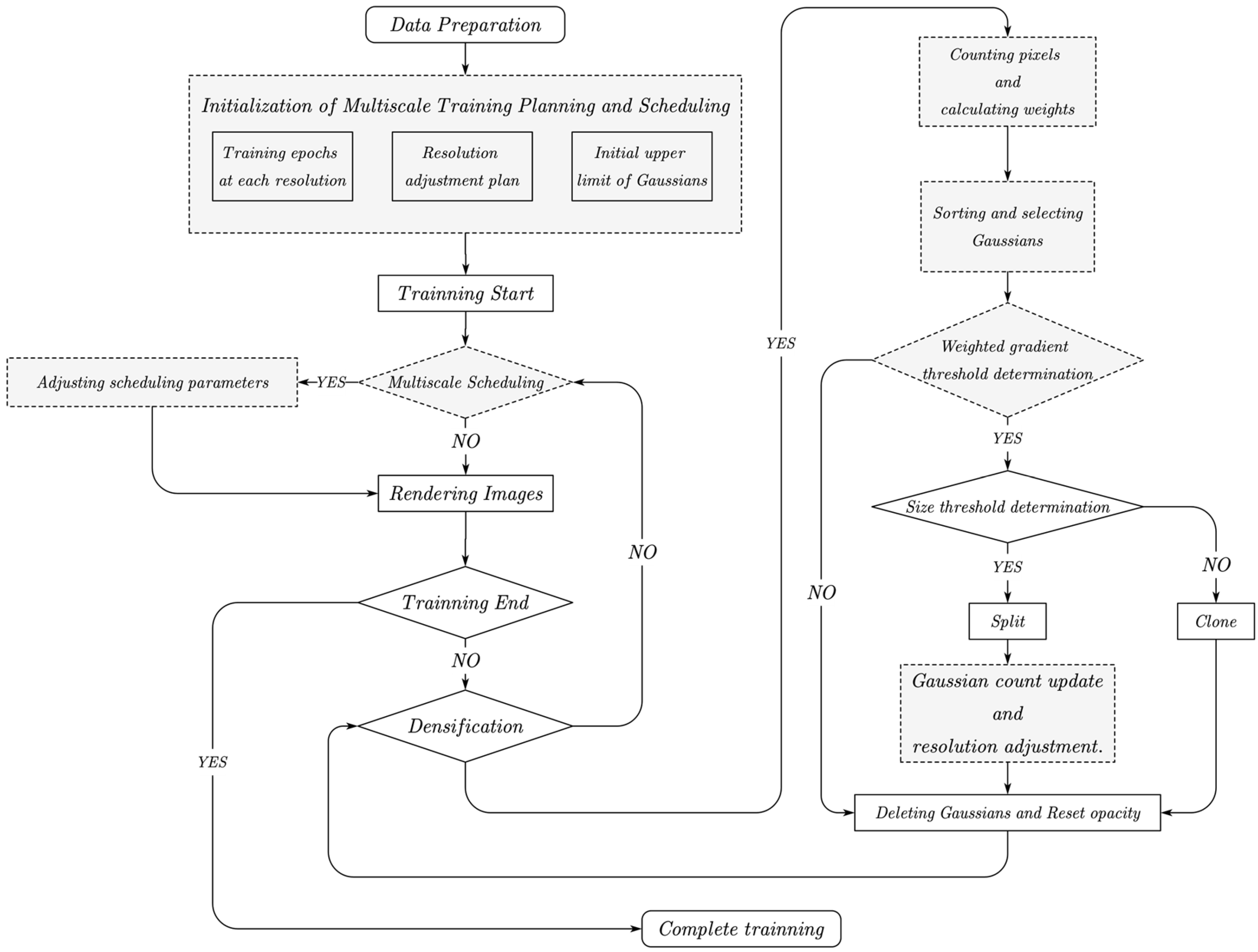
Based on these findings, an improved adaptive density control is proposed. This approach computes weights from the number of pixels covered by each Gaussian projection and applies them to the NDC-space position gradients. Without modifying any 3DGS hyperparameters, the algorithm guides Gaussians toward more stable and rational splitting and cloning behavior. Furthermore, by incorporating frequency-domain information, an adaptive multi-scale training scheduler is employed to reduce optimization time, thus enabling faster and higher-quality 3DGS reconstruction on each subregion. Figure 3 shows the workflow of the improved adaptive density.

4.3.1. Adaptive Density Control Based on Pixel-Weight Scaling

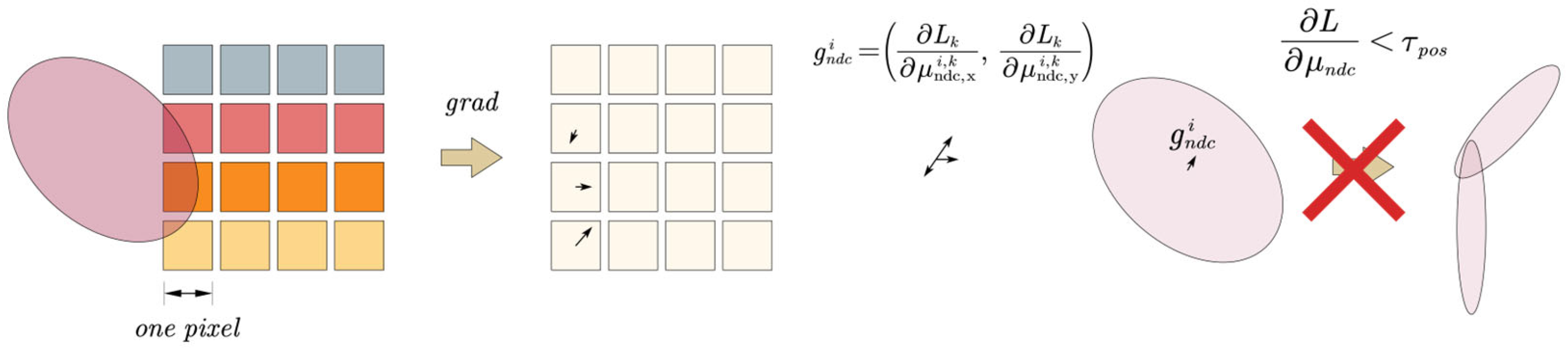
During rendering, the NDC-space gradients contributed by each image to the 3D Gaussians depend on transmittance and the spatial relationship between the projected center and the image plane. The most direct way to enhance transmittance is by capturing images from more diverse viewpoints. However, it requires pre-flight trajectory planning, which significantly increases both flight time and processing cost. To overcome this limitation, this section focuses on the effect of the projected center μ p i , k of each Gaussian primitive G 3 D i on the image plane I k . When μ p i , k lies outside the image boundary yet still contributes to rendering (as illustrated in Figure 4), the primitive affects only a small number of edge pixels. Consequently, the NDC gradient magnitudes returned by I k become extremely small, lowering the average gradient and preventing densification from being activated.
In the original 3DGS framework, the average-gradient-based control condition is expressed as:
∑ k = 1 M i ∂ L k ∂ μ n d c i , k 2 M i > τ p o s , τ p o s = 0.0002
where the numerator accumulates the NDC gradient magnitudes over one ADC interval period, and M i denotes the number of images participating in the densification simultaneously.
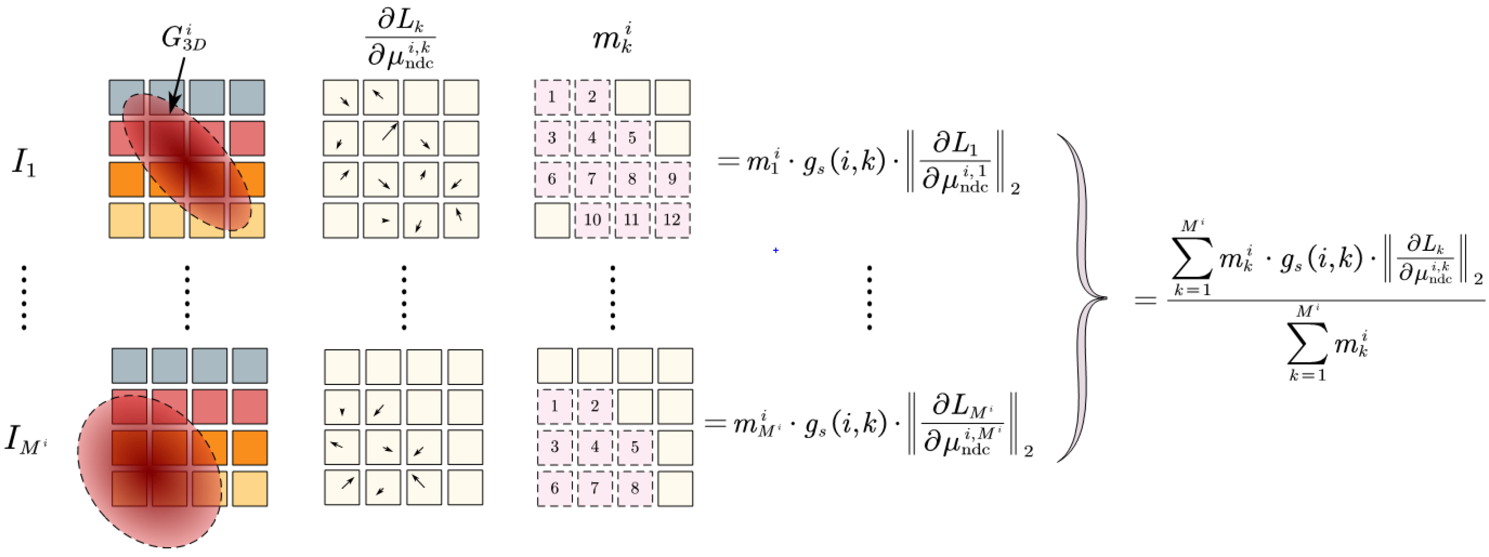
To mitigate the imbalance arising from variations in pixel coverage, a weighting factor proportional to the number of pixels contributing to each gradient computation is introduced. For large Gaussians, whose projected areas vary significantly across views, this weighting ensures that the resulting gradients are representative of their overall geometric behavior, thus triggering splitting or cloning only when necessary. For small ones, where pixel counts remain stable, the effect is minimal, avoiding unnecessary deviations or memory cost. The revised control condition is:
∑ k = 1 M i m k i ⋅ ∂ L k ∂ μ n d c i , k 2 ∑ k = 1 M i m k i > τ p o s
where m k i represents the number of pixels in image I k which contribute to the gradient computation for Gaussian i .
However, this weighting scheme introduces a potential drawback: Gaussians located near the camera may receive excessively large gradients, as they are generally unoccluded and already exhibit strong gradient responses. When further amplified by the weighting term, such primitives tend to over-split or over-clone, leading to floating artifacts in the reconstructed scene. To mitigate this effect, we introduce a spatial gradient-scaling factor g s i , k , which adjusts the gradient magnitude according to the scene depth and spatial scale. The final control condition is formulated as:
∑ k = 1 M i m k i ⋅ g s i , k ⋅ ∂ L k ∂ μ n d c i , k 2 ∑ k = 1 M i m k i > τ p o s
The scene-scale ratio r is defined based on camera distribution as:
r = 1.1 ⋅ m a x i C i − 1 N ∑ m = 1 N C m 2
where C m denotes the world-coordinate position of the m-th camera. The scaling factor g s i , k is then defined as:
g s i , k = F c l i p μ c a m , z i , k γ d e p t h × r 2 , 0 , 1
Here, μ c a m , z i , k represents the z-coordinate of Gaussian i in the camera coordinate system of image I k , and γ d e p t h is a depth-related hyperparameter, empirically set to 0.23 in the following experiments. Figure 5 illustrates the computational flow of the proposed adaptive density control.
The above formulation shows that the proposed pixel-weight scaling directly compensates for the imbalance in gradient accumulation caused by view-dependent pixel coverage. As analyzed in the Supplementary Materials, large primitives frequently appear only near image borders, where most pixels lie far from the projected Gaussian center and therefore contribute almost no gradients, even though these Gaussians still dominate the local geometry. As a result, the original average-gradient criterion may underestimate their importance and trigger inappropriate densification decisions. By weighting the gradients with the number of contributing pixels, the proposed control condition more faithfully reflects the effective spatial support of each primitive and activates splitting or cloning only when a Gaussian consistently occupies a sufficiently large image area across views. Small Gaussians, whose pixel support remains stable, are almost unaffected, which avoids unnecessary densification and memory overhead.
Pixel-weight scaling is adopted instead of alpha-based or occupancy-grid-based strategies for two main reasons. First, pixel counts can be obtained directly from the existing rasterization pipeline without maintaining an explicit 3D grid, which can be incorporated directly into the existing gradient computation without introducing additional volumetric data structures. Second, alpha values mainly encode local opacity along individual rays, whereas pixel coverage reflects the aggregate 2D support of a Gaussian over the image plane and is therefore more sensitive to the coverage imbalance caused by oblique views and boundary projections. The general idea of using the number of covered pixels as weights in the density growth condition has already been investigated in Pixel-GS [45], where a pixel-aware gradient is shown to improve density control, reduce floaters and enhance reconstruction quality on Mip-NeRF 360 and Tanks & Temples while preserving real-time rendering. Building on this prior evidence, the adaptive density control mechanism in this work adopts a similar pixel-coverage weighting but tailors the formulation to large-scale UAV scenes and integrates it with frequency-domain multi-scale scheduling and optimization, enabling efficient training on large-scale datasets.

4.3.2. Adaptive Multi-Scale Training Scheduling Strategy

Although the proposed adaptive density control in Section 4.3.1 provides a more rational criterion for densification, subsequent experiments reveal a decline in training efficiency, as summarized in Table 2.
Table 2 reports that the pixel-weight-scaled ADC increases the number of Gaussians from 9.19 M to 15.83 M and prolongs training time from 4362.28 s to 6320.63 s on the Mill 19 dataset. These indicate that the pixel-weight-scaled ADC generates more Gaussians but exhibits lower training efficiency, limiting its applicability to large-scale scene reconstruction under resource or time constraints. Existing 3DGS acceleration approaches primarily focus on (1) improving the rendering pipeline for faster convergence and (2) pruning redundant parameters during densification to improve computational efficiency. While these methods provide notable performance gains, excessive pruning often leads to a decline in reconstruction quality. Furthermore, high-resolution rendering during the early sparse phase introduces significant computational overhead, whereas the late-stage proliferation of Gaussians increases training cost with marginal quality improvement [46].
A more efficient alternative is multi-scale guided adaptive training. Here, “multi-scale” refers specifically to a progressive multi-resolution image-level training schedule (coarse-to-fine over increasing rendering/supervision resolutions). Under this setting, optimization proceeds across multiple levels of detail defined by image resolution scales. However, existing multi-scale methods typically require manual configuration of resolution hierarchies and iteration schedules, thereby increasing optimization complexity and prolonging training time. Moreover, supervising with low-resolution images while rendering at high-resolution often causes 3D aliasing artifacts [33], compromising both training stability and visual fidelity.
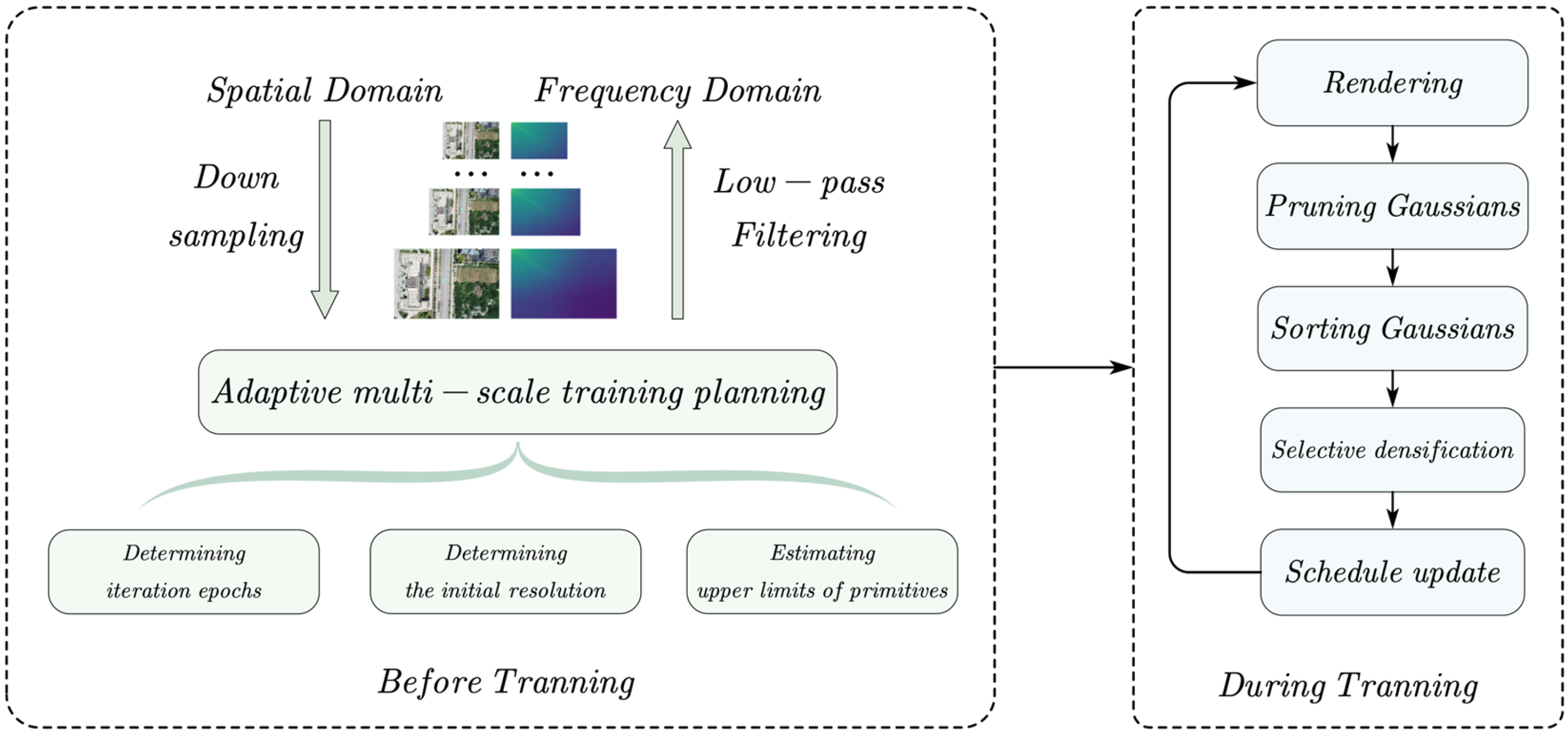
To overcome these limitations, an adaptive multi-scale scheduling strategy that transitions optimization from the spatial to the frequency domain is introduced. In frequency domain, low-frequency components encode global structure, whereas high-frequency components capture fine textures and details. Since the transformation between spatial and frequency domains is theoretically reversible, frequency differences provide a principled criterion for constructing a coarse-to-fine resolution schedule, forming the foundation of the optimization framework.
The key idea is to leverage frequency-domain variations to adaptively adjust image resolution and achieve progressive refinement of the reconstruction. Training starts with low-resolution rendering and supervision to capture coarse geometric structures and accelerate convergence. Prior to training, spectral analysis is used to determine the initial resolution and the iteration interval of each stage. During training, higher resolutions are introduced sequentially according to this predefined schedule to refine high-frequency details. Throughout the process, both the rendering resolution and the number of Gaussian primitives is dynamically adjusted, enabling efficient and progressive 3DGS optimization within single-GPU computational limits. The main components of the adaptive multi-scale scheduling framework are illustrated in Figure 6.
The core of the proposed training scheduling strategy lies in determining the optimal timing for rendering resolution adjustment. To this end, an image resolution saliency measure is defined, which provides a quantitative criterion for introducing higher-resolution images during training to refine image details at appropriate stages. The saliency is formulated as:
O T = 1 N ∑ n = 1 N ∑ i = 1 h ∑ j = 1 w | | F n ( i , j ) | | 2
where F n denotes the frequency-domain transform (e.g., Fourier or cosine transform) of training image I n ; I n n = 1 N represents the set of images sampled at a resolution of w , h ; and N is the total number of samples. Intuitively, when the ratio O T / O T r is much larger than the saliency value of the down-sampled image O T r , higher-resolution images should be introduced for supervision, and vice versa.
In practice, a sequence of monotonically decreasing down-sampling factors r 1 , r 2 , ⋯ , r m is employed. The corresponding downsampled images I r m , … , I r 1 , I are progressively incorporated into the supervision process during optimization. At iteration s r i , the rendering resolution is increased from H / r i , W / r i to H / r i − 1 , W / r i − 1 . To determine this scheduling, a ratio function [46] is defined as:
ϕ T , T r m , T r i = l o g O T / O T r i l o g O T / O T r m
If the total number of iterations is S , the iterations allocated to the image downsampled by factor r i are given by S ⋅ ϕ T , T r m , T r i .   Equivalently, at iteration s r , the resolution of the supervisory images should be increased from H / r , W / r to W , H , as expressed below:
s r i = S ⋅ 1 − ϕ T , T r m , T r i = S ⋅ l o g O T / O T r i l o g O T / O T r m
Because excessively dense Gaussians do not significantly improve rendering quality while increasing computational cost [37,47], the rendering resolution must be balanced with the number of Gaussian primitives. To achieve this balance, an adaptive upper bound on the maximum number of Gaussians per scene is therefore introduced. Let P i n i t and P f i n denote the initial and target numbers of Gaussians, respectively. The number of primitives at iteration i is defined as:
P i = P i n i t + P f i n − P i n i t r ( i ) 2 − i S
where r ( i ) is the rendering resolution at iteration i , and S is the total number of iterations. The exponent term 2 − i / S decreases from 2 to 1 as training progresses, suppressing early primitive growth while accelerating it in later stages, thereby reducing optimization complexity.
Unlike prior works [36], which fix P f i n as a constant multiple of P i n i t , a reward updating mechanism inspired by reinforcement learning is adopted. The previous estimate P f i n i − 1 is treated as a historical value, and the newly observed “incremental reward” P n e w i is combined to yield an optimal update via a max operation:
P f i n i = m a x P f i n i − 1 , γ ⋅ P f i n i − 1 + η ⋅ P n e w i
where γ and η are hyperparameters, and i denotes the iteration index. The max operation ensures monotonic growth of P f i n i during optimization. The parameter P f i n i is updated iteratively according to Equation (17), with the initial value set as P f i n 0 = 10 ⋅ P i n i t = 10.

5. Experiments and Discussion

5.1. Datasets and Metrics

5.1.1. Datasets

The experiments are conducted on six large-scale UAV datasets, with specific details available in Table 3.
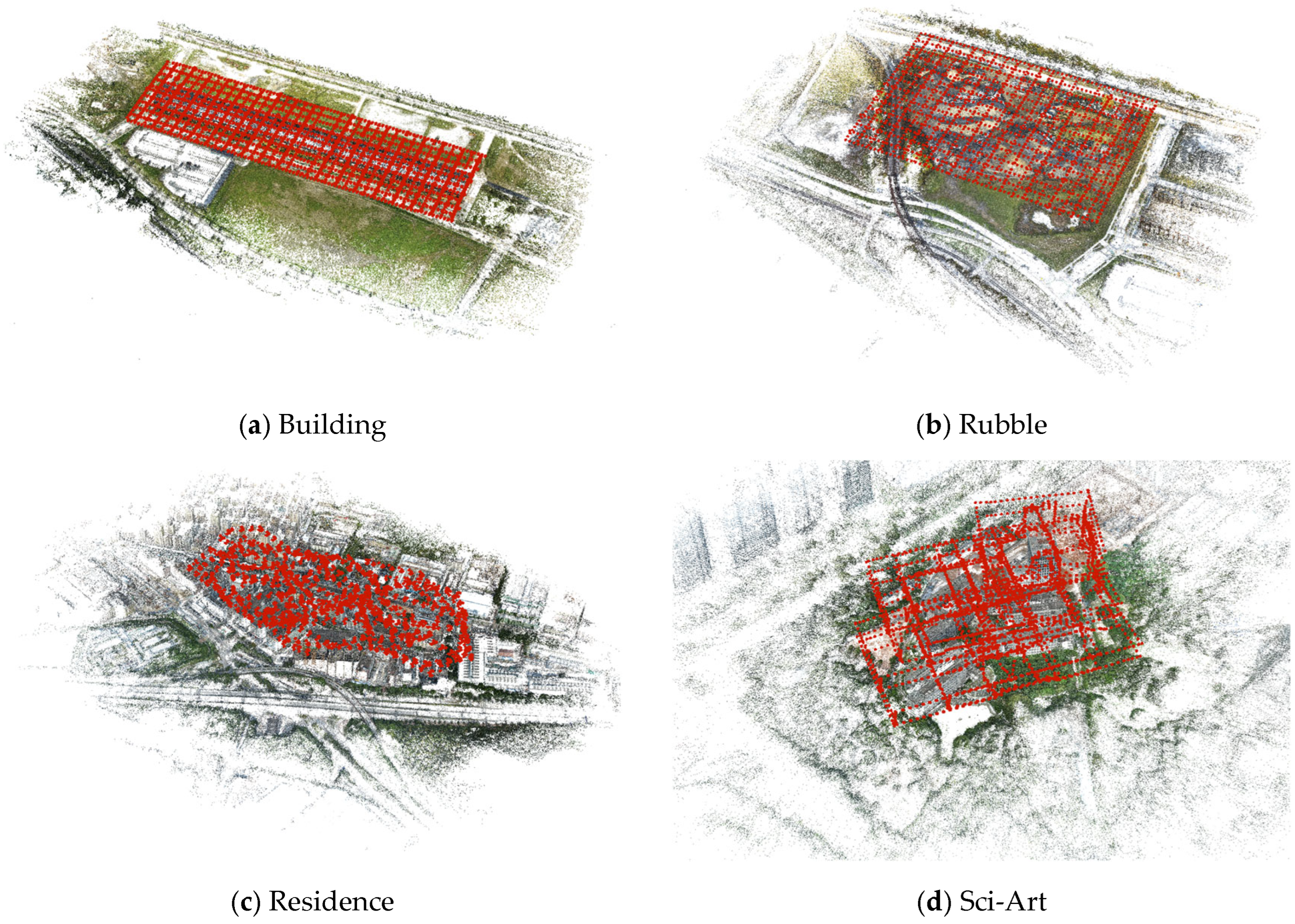
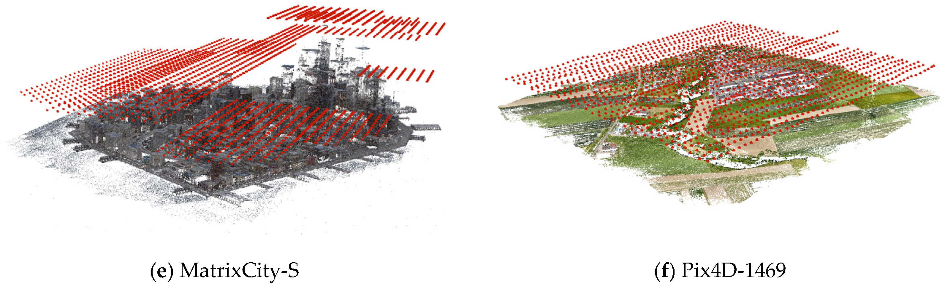
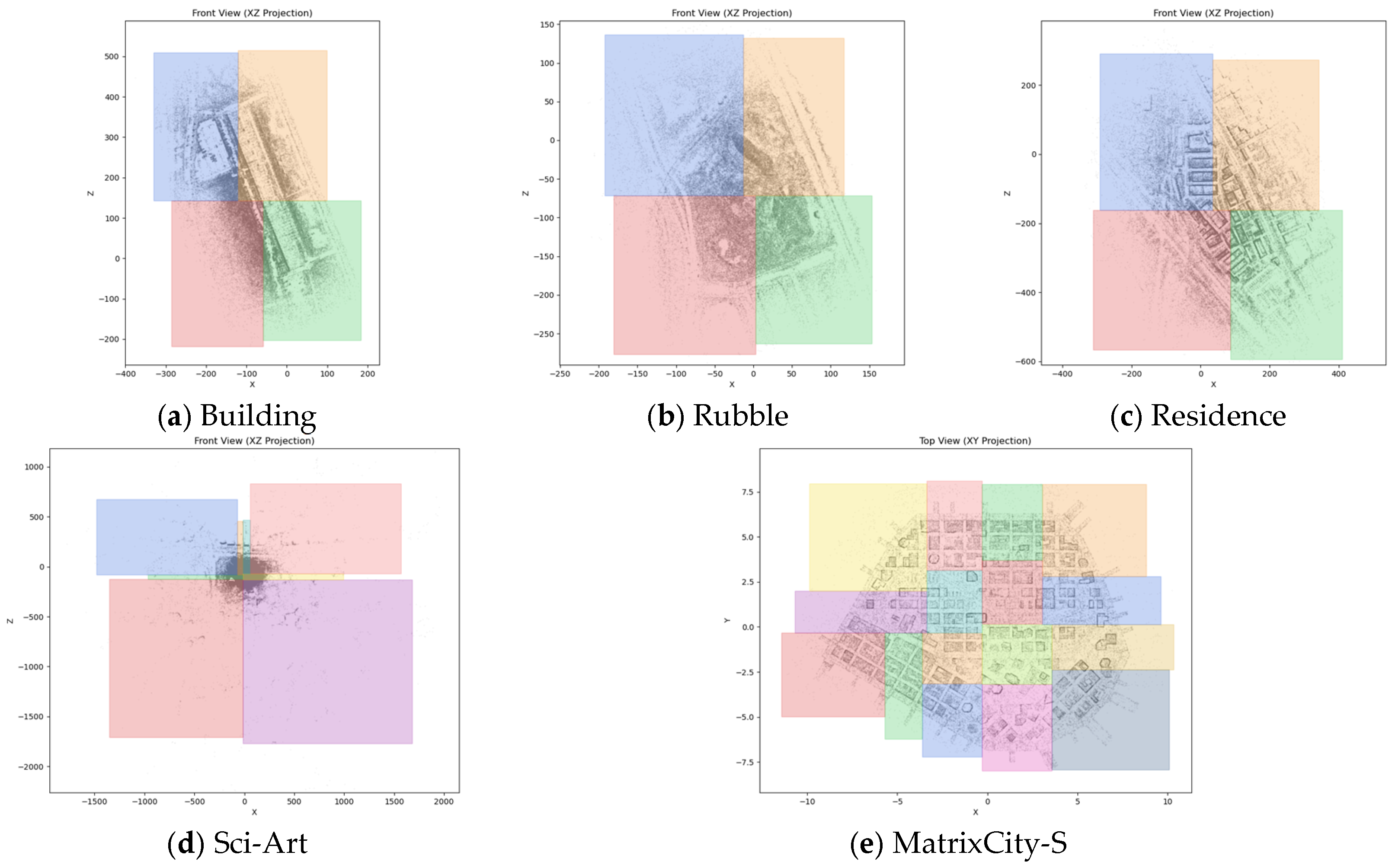
The Rubble and Building are sourced from the Mill 19 [4] dataset, which was released by the Carnegie Mellon University. It is widely used as benchmark for large-scale scene reconstruction tasks. The Mill 19 comprises two representative industrial scenes: an industrial building (Building) and an industrial ruin (Rubble). All images were captured using grid-based aerial trajectories, achieving a maximum resolution of 4608 × 3456 pixels. In this study, they are employed to assess the performance of the proposed method in a “regular flight route + industrial park” scenario. The layouts of the flight routes are illustrated in Figure 7a,b.
The Residence and Sci-Art are derived from the UrbanScene3D [48] dataset, which contains both real and synthetic urban imagery. The dataset comprises over 128,000 images across 16 distinct scenes, covering an area of approximately 136 km2. The two subsets used in this study correspond to urban residential areas and university campuses. Unlike the grid-based aerial trajectories in the Mill19 dataset, the UrbanScene3D dataset exhibits irregular UAV flight paths with greater viewpoint diversity, providing an effective means of evaluating the robustness of the proposed method under nonuniform viewpoint distributions and complex occlusion conditions. The detailed configurations of the flight paths are depicted in Figure 7c,d.
The MatrixCity [49] is jointly developed by the Chinese University of Hong Kong and the Shanghai Artificial Intelligence Laboratory. It provides various types of data, including RGB images, depth, and normal maps. In this study, only the Small City subset is utilized, referred to as MatrixCity-S. The dataset simulates an oblique-photography configuration with four orientations (front, back, left, and right), and the corresponding UAV flight-path layout is illustrated in Figure 7e.
All training and test sets from the public datasets strictly follow the official releases to ensure fairness and comparability across experiments.
Additionally, this study employs a sample photogrammetry dataset provided by Pix4D SA, hereafter referred as Pix4D-1469 [50]. This dataset comprises 1469 UAV images with a resolution of 5958 × 3972, covering industrial, residential, and agricultural areas. All images were captured following grid-pattern flight trajectories, as shown in Figure 7f. The training and test sets were randomly divided in a 10:1 ratio (see Table 3). Unlike previously introduced datasets, the camera orientations are predominantly nadir-facing (downward), and the significantly higher image resolution presents considerable challenges for Gaussian-based reconstruction methods in terms of both reconstruction quality and computational efficiency.

5.1.2. Metrics

To evaluate the performance of the proposed method, three quantitative metrics are employed:
Peak Signal-to-Noise Ratio (PSNR). PSNR measures pixel-level differences between two images by comparing the ratio of the maximum pixel value (MAX) to the mean squared error (MSE). It is defined as:
P S N R = 10 ⋅ l o g 10 M A X 2 M S E
A higher PSNR value indicates smaller pixel-wise reconstruction errors and thus better rendering fidelity.
Structural Similarity Index (SSIM). SSIM evaluates the perceptual similarity between two images in terms of luminance, contrast, and structure. The SSIM value ranges from −1 to 1, where a higher value denotes greater similarity. It is as follows:
S S I M x , y = 2 μ x μ y + C 1 2 σ x y + C 2 μ x 2 + μ y 2 + C 1 σ x 2 + σ y 2 + C 2
where μ x and μ y denote the mean intensities of the reference and rendered images, σ x 2 and σ y 2 represent their variances, σ x y is their covariance, and C 1 and C 2 are constants to prevent division by zero.
Learned Perceptual Image Patch Similarity (LPIPS). LPIPS quantifies perceptual similarity by leveraging convolutional neural networks to extract deep feature representations and computing the distance between corresponding features of two images. It is defined as:
d = ∑ l l H l W l ∑ h , w f x l ( h , w ) − f y l ( h , w ) 2 2
where f x l and f y l denote the features of images x and y at the l − t h layer, while H l and W l represent the height and width of the feature maps, respectively.

5.2. Training Details

The proposed framework is implemented in PyTorch 2.5.1 with CUDA 11.8 for parallel computation acceleration. All experiments are conducted on a workstation equipped with an Intel Xeon 6620R processor, 64 GB RAM, and a single NVIDIA RTX 3090 GPU (24 GB VRAM). Given that the RTX 3090, released in 2020, provides less than half the computational power of current mainstream GPUs (see Table 4), it serves as a representative platform for simulating resource-limited environments. The Adam optimizer was used to update model parameters, with the learning rate set to 1 × 10⁻⁴, β 1 = 0.9 and β 2 = 0.999 , following the default configuration of the original 3DGS.
The densification interval frequency is adjusted according to the dataset: 150 for Mill 19 and UrbanScene3D, 400 for MatrixCity-S, and 500 for Pix4D-1469. The densification iteration range is configured to [1000, 17,500], within a total of 35,000 training iterations. To balance training efficiency and reconstruction quality, the image down-sampling rate is set to 0.25. The subregion expansion rate is set to 5%, applied during subregion partitioning and stitching throughout training.
To validate the effectiveness of the proposed method, comparisons are made with several state-of-the-art approaches based on NeRF and 3DGS, including Mega-NeRF, Switch-NeRF, the original 3DGS (3DGS), CityGaussian (CityGS), and DOGS. The original 3DGS is trained using the default configuration provided in its official code repository. However, since DOGS and CityGS cannot be trained on a single GPU with 24 GB of VRAM under their default settings for certain scenes, their results are taken directly from the corresponding publications.
To further assess the training efficiency and reconstruction performance under single-GPU constrains, the proposed method is compared with the improved 3DGS (3DGS†) and BlockGaussian, both capable of single-GPU performance with competitive reconstruction quality. 3DGS† adopts the same partitioning strategy and training parameters as the proposed framework but excludes the improved adaptive density control mechanism. BlockGaussian follows the training protocol described in its original paper, with the densification iteration range set to [1000, 20,000], a total of 40,000 training iterations, and an image down-sampling rate of 0.25. Due to VRAM limitations, the densification interval frequency for BlockGaussian on the Pix4D-1469 dataset was adjusted from 200 to 750 preventing VRAM overflow during training. All experiments in this group are conducted on a single NVIDIA RTX 3090 GPU. The configuration details of the above methods, presented in a more intuitive manner, can be found in Table 5.

5.3. Comparison with Other Methods

5.3.1. Quantitative and Visual Comparison of Different Methods

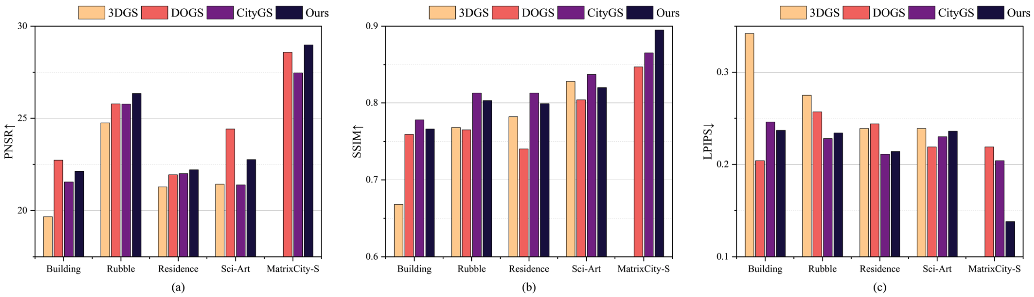
Table 6, Table 7 and Table 8 and Figure 8 present the quantitative comparison results. The two NeRF-based methods achieve higher PSNR values, but their performances in the other two metrics are inferior to 3DGS-based methods, indicating limited capability in restoring fine structural details. Furthermore, their training times are significantly longer than that of the original 3DGS. In contrast, the 3DGS-based methods consistently demonstrate efficient and stable performance across all datasets. Except for Sci-Art, the proposed method surpasses the NeRF-based reconstruction approaches on all evaluation metrics. It achieves the highest PSNR among the 3DGS-based methods and ranks second in SSIM and LPIPS. Notably, on the MatrixCity-S dataset (>6000 images), training with the proposed method is finished on a single 24-GB GPU in less than 60% of DOGS’s time, and higher scores were obtained on all three metrics.
In terms of overall performance on the evaluated UAV datasets, the proposed method achieves reconstruction accuracy that is comparable to Gaussian-splatting approaches relying on multi-GPU parallel training. At the same time, it can be trained efficiently on a single GPU, making it particularly suitable for environments with limited computational resources. Although the training time remains close to that of the original 3DGS implementation, this does not mean that the introduced components have no impact on efficiency. Table 2 shows that, when the pixel-weight-scaled ADC is applied in isolation on Mill-19, the number of Gaussians increases from 9.19 M to 15.83 M and the training time grows from 4362.28 s to 6320.63 s (≈1.45×). This confirms that the refined density control is the main source of additional computational load. By comparison, the content-adaptive partition training strategy introduces only a modest overhead on the smaller scenes: Table 6 reports that the proposed method differs from the original 3DGS by only a few minutes on the Building (01 h 29 min vs. 01 h 31 min) and Rubble (01 h 35 min vs. 01 h 26 min) datasets, while Table 7 shows a similar gap on the Residence dataset (01 h 49 min vs. 01 h 42 min). On the more complex Sci-Art scene, the method attains higher PSNR and lower LPIPS than 3DGS, but the training time increases more noticeably (from 00 h 53 min to 03 h 11 min), which is consistent with the larger number of Gaussians required to represent highly intricate structures. For the very large MatrixCity-S dataset, Table 8 and Figure 8 highlight a different regime: the standard 3DGS cannot complete training on a single 24-GB GPU, whereas the proposed method finishes in 02 h 41 min and yields the best PSNR, SSIM and LPIPS among all 3DGS-based approaches, while still using less than 60% of DOGS’s training time. These results indicate that on small and medium-scale Geographical scenes the extra cost introduced by the more accurate ADC is largely compensated by improved load balancing and resource usage, so the total training time stays close to that of standard 3DGS, whereas on large-scale scenes the same design yields clear advantages in terms of scalability and wall-clock time.
It is worth noting that on Sci-Art, the PSNR of the NeRF-based methods is slightly higher than that of the 3DGS-based ones. This difference, however, primarily reflects smaller pixel-level errors rather than superior perceptual quality. The 3DGS-based approaches produce renderings that better align with human visual perception, as evidenced by higher SSIM and lower LPIPS. Regarding training time, 3DGS, owing to their holistic training strategy, are substantially faster than all other reconstruction approaches.
Nevertheless, the proposed single-GPU framework does not achieve the best score in every metric and on every scene. For example, on the Building scene, DOGS attains slightly higher PSNR and lower LPIPS than our method, while on the Sci-Art scene CityGS provides the highest SSIM among 3DGS-based approaches. These differences are mainly related to the design choices made for single-GPU scalability: the content-adaptive partitioning and conservative density-control strategy limit the maximum number of Gaussians that can be assigned to each subregion and enforce strictly sequential training, which can result in mildly smoother reconstructions and slightly under-fitted high-frequency details in the most complex areas. In contrast, methods such as DOGS and CityGS are designed for distributed or multi-GPU training and can handle very large-scale scenes with massive numbers of Gaussians through block-wise parallel optimization and subsequent fusion, but at the cost of relying on more complex multi-GPU hardware which is less accessible in strictly single-GPU environments.
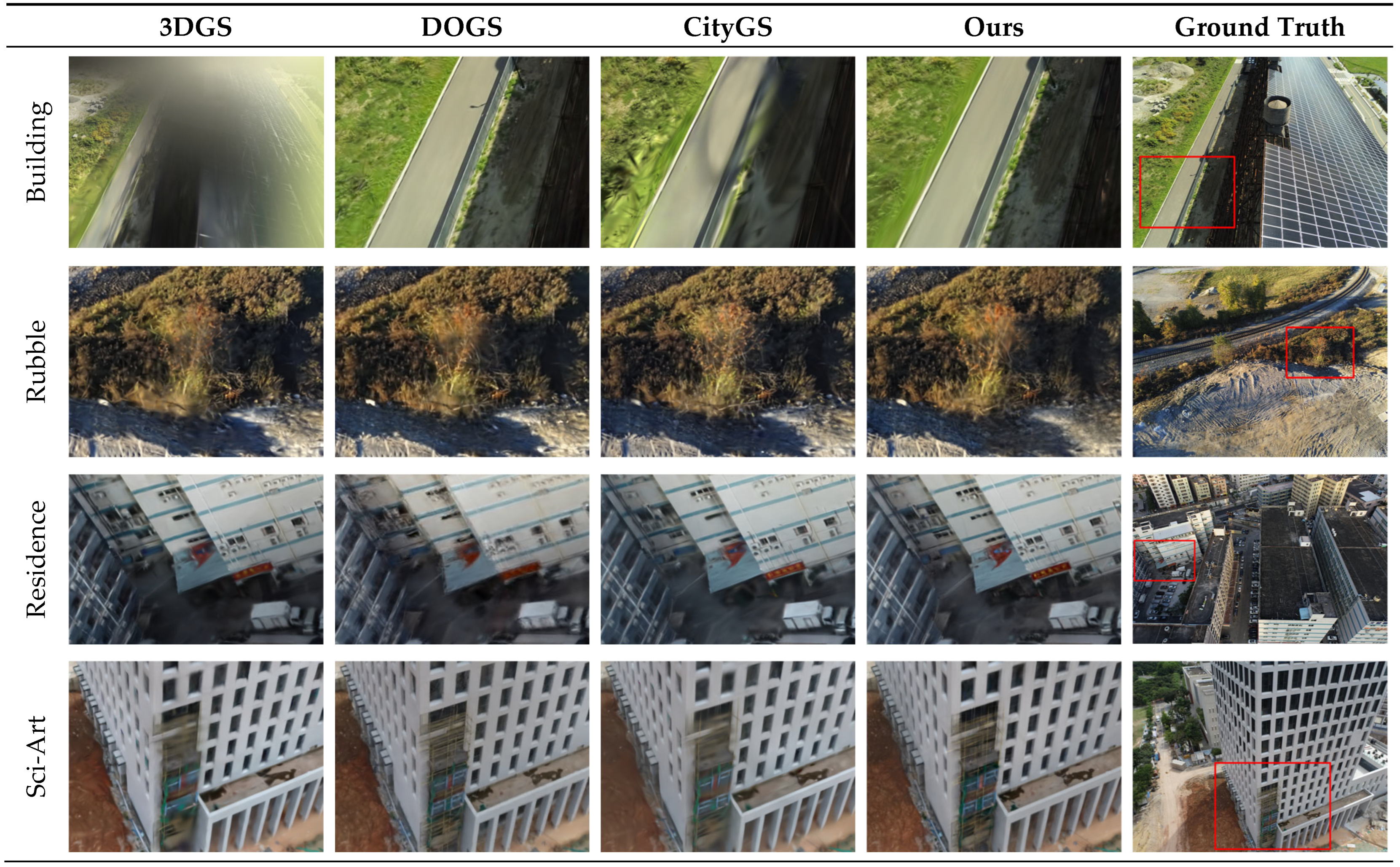
From a qualitative perspective, Figure 9 presents representative visual results obtained after training on different datasets. The selected samples contain regions with intricate details—such as rooftops with reflective surfaces and buildings of varying heights or dislocated structures—that pose significant challenges due to their geometric and textural complexity.
The visualization results show that 3DGS performs poorly in regions with large, uniform textures, such as the solar roof in the Building dataset. It produces noticeable artifacts and fails to adequately restore local details (e.g., the red tarpaulin in the Residence dataset and the scaffolding in the Sci-Art dataset). These deficiencies arise because the adaptive density control in 3DGS does not effectively guide the splitting of Gaussians, leading to suboptimal fitting and the loss of high-frequency details; consequently, the final renderings appear blurred. In contrast, DOGS and CityGS exhibit substantial improvements in detail reconstruction, as highlighted by the red boxes in Figure 9. Nevertheless, some residual blurriness (e.g., DOGS in the Residence dataset) and artifacts (e.g., CityGS in the Building dataset) remain. The proposed method, equipped with the improved adaptive density control mechanism, achieves superior visual fidelity, reproducing finer structural details without perceptible color bias or blurriness. Moreover, renderings from novel viewpoints demonstrate higher geometric consistency and visual accuracy, further validating the robustness of the proposed approach.

5.3.2. Efficiency and Consumption

To further assess the effectiveness of the proposed method in managing computational resources, comparisons were conducted with BlockGaussian, which performs effectively on a single GPU (RTX 3090), and the improved 3DGS employing a scene-complexity-based partitioning strategy (3DGS†). Comparative experiments are conducted on five datasets, with all methods trained sequentially by subregions. Table 9 and Table 10 present the quantitative results. The PSNR values differences among three methods do not exceed ±0.65, while the SSIM and LPIPS differences remain within ±0.019, indicating that the rendering quality is nearly identical.
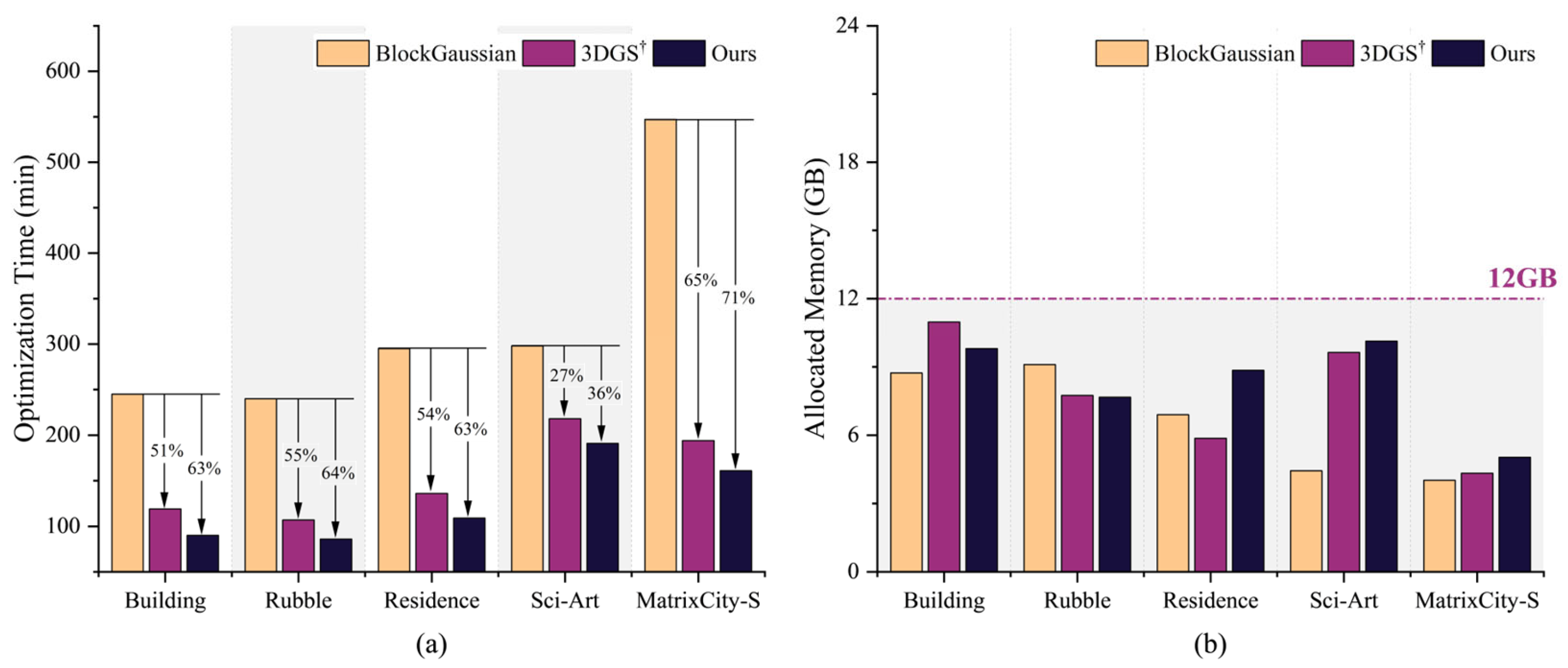
However, Figure 10a reveals a substantial reduction in total training time for both 3DGS† and the proposed method. The most pronounced improvement is observed on the MatrixCity-S dataset, which contains more than 6000 images: 3DGS† and the proposed method reduce training time by 65% and 71% compared with BlockGaussian, respectively. Furthermore, Figure 10b shows that the peak VRAM consumption during subregion training for all three methods remains below 12 GB, underscoring the superior computational efficiency of the proposed approach.
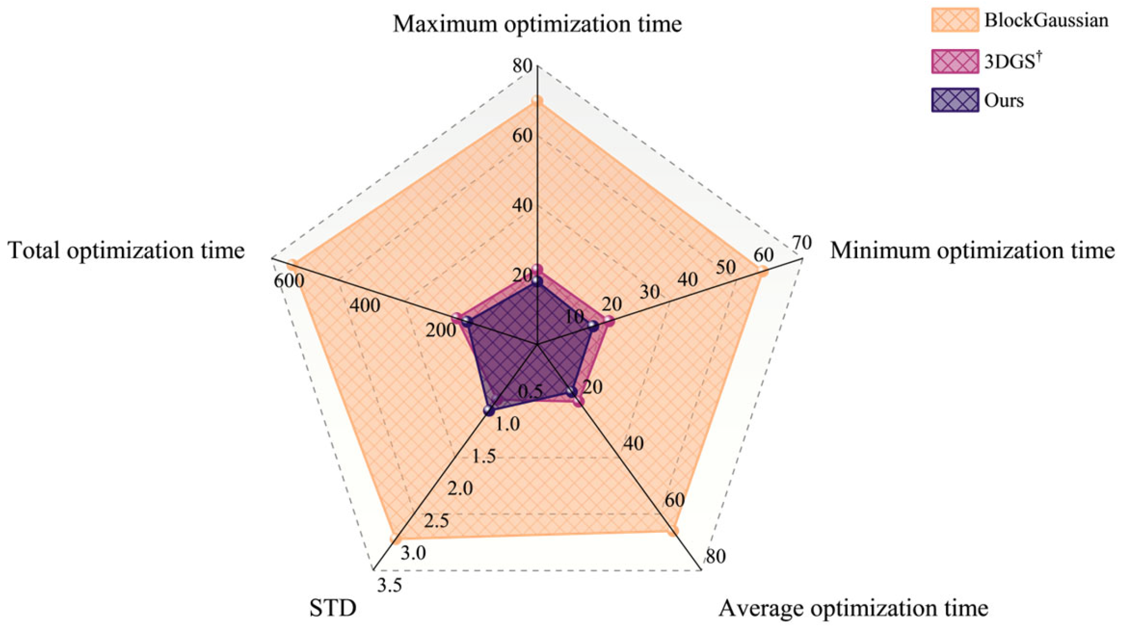
To further assess practicality, we evaluate all three methods on the Pix4D-1469 photogrammetry dataset, whose high resolution, sparse viewpoints, and large data volume impose heavy computational demands on Gaussian-Splatting-based approaches. As summarized in Table 11, BlockGaussian successfully completes subregion training but fails at model merging and rendering due to an out-of-memory (OOM) error, and thus cannot finish the test. In contrast, both 3DGS† and the proposed method exhibit markedly improved efficiency, reducing total training time by 428 min and 451 min compared with BlockGaussian, respectively. In addition, the proposed method also achieves the lowest peak VRAM usage during subregion training (approximately 36.89% lower than that of BlockGaussian) demonstrating superior performance advantage in memory efficiency. Moreover, the proposed method exhibits more balanced computational performance across subregions. As illustrated in Figure 11, the standard deviation (STD) of optimization time per subregion is below 1.5, which is less than half of that observed in BlockGaussian. This indicates that the proposed scene-complexity-based partitioning and view assignment scheme achieves a more uniform per-subregion optimization time, i.e., a better balance computational load across blocks, which in turn improves overall training stability and efficiency.

5.4. Ablation Studies

This section presents ablation studies of the content-adaptive partitioning strategy and the improved adaptive density control mechanism, quantifying each key component’s contribution to the proposed framework’s overall performance.

5.4.1. Evaluation of the Content-Adaptive Partitioning Strategy

Table 12 and Figure 12 present the partition statistics and the corresponding visualization results, respectively. In Table 12, N b l o c k s denotes the number of partitions; N i m a g e s m e a n and N i m a g e s s t d represent the mean and standard deviation of the number of images per subregion; N s f m m e a n and N s f m s t d denote the mean and standard deviation of the number of initial sparse points per subregion (unit: points); and T o p t t o t a l and T o p t s t d correspond to the total training time for all subregions (in seconds) and the standard deviation of training time per subregion, respectively. To compare relative dispersion across scenes of different scales, the coefficient of variation is additionally reported as C V = s t d / m e a n , which is a standard, unitless measure of relative variability.
The proposed content-adaptive partitioning strategy estimates scene complexity from the initial sparse SfM point distribution, producing subregions with comparable geometric content. This is reflected by consistently small N s f m s t d and low C V ( N s f m ) for most scenes, indicating that complexity-adaptive splitting keeps the amount of sparse content per subregion within a similar range. Meanwhile, view assignment based on subregion–camera correlation maintains balanced supervision: N i m a g e s s t d remains low and C V ( N i m a g e s ) stays small for Building, Rubble, and Residence, showing that training images are distributed evenly across subregions. Although Sci-Art exhibits larger dispersion in both images and sparse points due to highly heterogeneous structures, the variation in optimization time is still well controlled. In particular, T o p t s t d is small relative to the mean per-subregion training time, and C V ( T o p t ) remains low across all datasets. These results indicate that the partitioning and correlation-based image allocation jointly balance per-subregion computational load, leading to similar memory footprint and training time during sequential single-GPU optimization. Figure 12 provides a visual illustration of the adaptive partitioning results across different datasets.

5.4.2. Quantitative Results of Partition Training

To further evaluate the contribution of each component within the partition training strategy, ablation experiments were conducted on the Building dataset. Table 13 summarizes the results. The original 3DGS algorithm—without partitioning or a dedicated training strategy—achieves a PSNR of 19.67, an SSIM of 0.668, and an LPIPS of 0.342. Incorporating the proposed partitioning strategy and auxiliary point cloud-based subregion training improves performance across all metrics. Specifically, PSNR increases by 8.49% and 12.46%, SSIM improves by 9.13% and 14.67%, and LPIPS decreases by 23.68% and 30.70%, respectively.
In terms of time efficiency, the full method requires only 2.30% more training time than the original 3DGS while reducing memory consumption by 35.11%. These results confirm that the proposed partition training strategy achieves an effective balance between computational efficiency and rendering quality.

5.4.3. Evaluation of the Improved Adaptive Density Control

To directly compare the improved ADC mechanism with the original gradient-based densification in 3DGS, ablation experiments were conducted on the Rubble dataset, with results summarized in Table 14. Using only the weight-scaling method yields the highest performance across all metrics, with PSNR increasing by 1.66%, SSIM improving by 2.53%, and LPIPS decreasing by 19.38% relative to the original gradient-based ADC baseline. However, this configuration extends optimization time to 1.45× that of the baseline.
In contrast, the adaptive multi-scale training approach requires only 81% of the baseline training time but produces a noticeable degradation in rendering quality, indicating the adverse influence of multi-scale image training on Gaussian model fidelity. The full method proposed in this study increases training time by only 18% relative to the baseline while maintaining high rendering quality. The most substantial gain is observed in LPIPS, which decreases by 19.03%, achieving results comparable to those of the weight-scaling method alone.
These ablation results and the statistics in Table 1 together clarify the improvements introduced by the pixel-weighted adaptive density control compared with the original gradient-based densification in 3DGS. On the Rubble dataset, replacing the original ADC with the pixel-weighted variant increases the number of Gaussians and leads to a longer training time, but also enables a more faithful recovery of fine-scale geometry. On the Rubble dataset, using only the weight-scaling component yields the best quantitative performance across all metrics: PSNR and SSIM show noticeable gains, while LPIPS decreases substantially relative to the baseline. These improvements indicate that the pixel-weighted gradients enhance densification precision by allocating additional primitives to regions where the original average-gradient criterion fails to trigger splitting, such as sparsely textured surfaces and oblique boundary projections. Taken together with the visual comparison in Figure 13, these findings confirm that the pixel-weighted adaptive density control not only improves quantitative accuracy metrics but also effectively suppresses floating artifacts that frequently occur under the original gradient-based densification rule.
At the same time, the adaptive multi-scale training strategy effectively compensates for the additional computational cost introduced by the pixel-weighted ADC. Although using pixel-weight scaling alone increases the optimization time by a considerable factor, the full method reduces this overhead while preserving almost all of the LPIPS gain. In other words, the resulting ADC mechanism not only improves the visual fidelity of large-scale reconstructions but also maintains a favorable trade-off between reconstruction quality and training efficiency under single-GPU hardware constraints.

5.4.4. Qualitative Comparison

To visually demonstrate the impact of the proposed improvement, a qualitative comparison was performed between the original ADC-trained 3DGS and the proposed method. Both methods employed the same partitioning strategy introduced in this study to ensure fairness, and the visualizations were generated by using SuperSplat [52] platform.
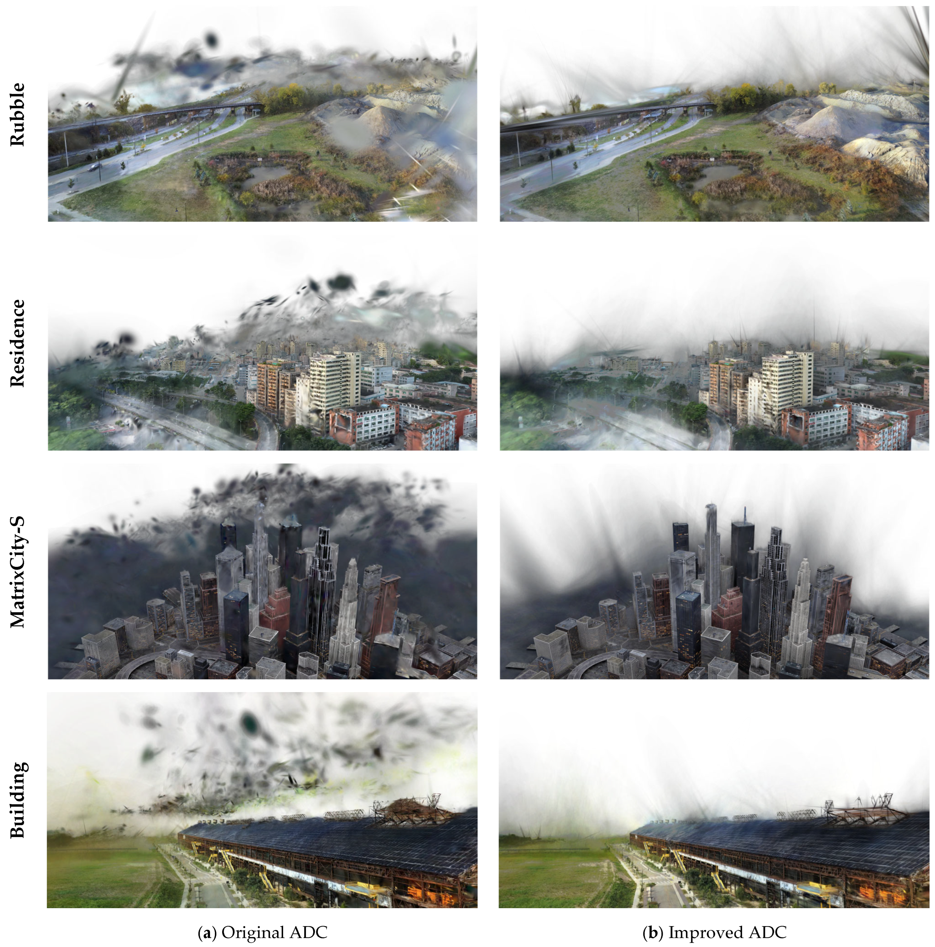
As shown in Figure 13, the original ADC method computes the densification threshold based on the average gradient, which can incorrectly trigger the densification of Gaussians which do not meet the required conditions. This produces floating artifacts, particularly when large Gaussians are visible from multiple viewpoints. The projected area of these Gaussians varies substantially across different perspectives, resulting in inconsistent pixel contributions to the gradient calculation. Mathematically, pixels near the center of the projection contribute more strongly than those near the periphery. When projection centers fall outside the screen space, the average gradient decreases, leading to erroneous splitting or replication of Gaussians.
The improved ADC effectively mitigates this issue, significantly reducing the occurrence of floating artifacts. This improvement is particularly evident in regions with sparse textures, such as the water bodies in the MatrixCity-S scene and black solar panels on factory rooftops in the Building scene. Considering both quantitative and qualitative results, the proposed ADC mechanism enhances rendering fidelity while incurring only a marginal increase in training time. It achieves an excellent balance between precision and efficiency, maintaining low computational resource consumption and demonstrating strong practical applicability.

6. Conclusions

This study proposes a new framework for large-scale scene reconstruction leveraging 3D Gaussian Splatting under limited hardware conditions. It addresses the high computational cost and suboptimal reconstruction quality of traditional 3DGS methods in large-scale scenarios by focusing on two key aspects: balanced scene partitioning and optimized adaptive density control. First, scene complexity is estimated from the initial sparse point clouds, and a scene-complexity-based partitioning strategy is developed to balance the computational load across subregions. During training, only the point cloud within each subregion is densified, while the auxiliary point cloud outside the subregion only learns color information, avoiding unnecessary splitting or replication. This design effectively reduces resource consumption while maintaining scene integrity and perceptual continuity.
Second, an improved adaptive density control (ADC) mechanism is introduced to overcome the limitations of gradient-based densification in original 3DGS. A pixel-weighted gradient computation is proposed to account for the number of contributing pixels, thereby enhancing densification precision. Additionally, a frequency-domain adaptive multiscale training strategy is incorporated to construct a multiresolution optimization process. This strategy suppresses excessive Gaussian growth during early low-resolution stages and promotes controlled refinement in later high-resolution phases, improving optimization efficiency while preserving rendering quality. Previous methods such as Pixel-GS have already demonstrated that incorporating pixel-aware gradients into the density growth condition can effectively enhance 3DGS reconstructions and suppress floaters on standard benchmarks. In contrast, the present framework extends this strategy to large-scale UAV reconstruction and couples it with a frequency-domain adaptive multi-scale training schedule and improved density control, thereby achieving a favorable balance between reconstruction fidelity, Gaussian count and training efficiency under single-GPU constraints.
Finally, comprehensive experiments on various datasets demonstrate that the proposed method can reconstruct a 1.2 km2 scene only in 144 min on a single RTX 3090 GPU (24 GB VRAM). Compared with existing approaches, it achieves comparable or superior rendering quality while reducing optimization time by more than 50% and maintaining VRAM usage below 12 GB. These achievements make it highly suitable for deployment under resource-constrained environments, with strong potential for applications such as emergency rescue and urban digitization.
Overall, the comparative analysis indicates that no single reconstruction method consistently outperforms others across all objectives. While NeRF-based approaches tend to achieve slightly higher PSNR in certain scenes, they require significantly longer training times and generally yield poorer SSIM and LPIPS scores. These limitations reduce their practicality for large-scale UAV mapping. On the other hand, standard 3DGS models and multi-GPU variants, such as DOGS and CityGaussian, produce high-quality reconstructions with real-time rendering capabilities. However, they either necessitate expensive multi-GPU hardware or face challenges such as memory overflow and quality degradation when applied to kilometer-scale scenes. In contrast, the proposed single-GPU framework strikes a favorable balance between reconstruction accuracy, training time, and hardware requirements, making it particularly well-suited for large-scale static urban and industrial environments with limited computing resources.
Despite these advantages, several limitations remain and suggest directions for future work. First, the pixel-weight-scaled adaptive density control still increases the number of Gaussians and prolongs training on some datasets, even with the proposed multi-scale schedule, which enlarges the model size and storage cost. A natural next step is to couple the current densification rule with more conservative, structure-aware pruning, or to compress the final Gaussian representation into more compact explicit forms (such as meshes or voxels), so as to further reduce the memory footprint in very large scenes. Second, the present framework is only evaluated on static UAV imagery acquired by a single RGB sensor and does not explicitly model temporal changes or cross-sensor cues. Extending the partitioning and density-control mechanisms to multi-temporal image sequences and multimodal inputs (e.g., RGB with LiDAR or combined nadir/oblique imagery) is important for applications that require change monitoring or 4D scene reconstruction. Likewise, the frequency-based multi-scale scheduling strategy introduced in this work is not restricted to Gaussian splatting; future work will explore adapting it to NeRF-based pipelines to examine whether similar reductions in training time can be achieved without sacrificing fine details. These directions may help mitigate some of the current weaknesses of both NeRF- and 3DGS-based large-scale reconstruction methods and broaden the applicability of the proposed framework.

Supplementary Materials

The following supporting information can be downloaded at: https://www.mdpi.com/article/10.3390/rs17233868/s1, Figure S1: Diagram of variable dependencies in NDC-space gradient computation; Figure S2: Illustration of gradient variations of Gaussians sampled along a single ray by depth order; Figure S3: Coverage relationships among Gaussians at image boundaries; Figure S4: Comparison of orbit-based and grid-flight data acquisition schemes.

Author Contributions

Conceptualization, K.Y. and H.W.; methodology, K.Y.; software, K.Y. and Z.L.; validation, Y.W.; formal analysis, H.W. and Z.L.; investigation, K.Y.; resources, S.L.; data curation, S.L.; writing—original draft preparation, K.Y.; writing—review & editing, K.Y. and H.W.; visualization, H.Y.; supervision, S.L. All authors have read and agreed to the published version of the manuscript.

Funding

This research received no external funding.

Data Availability Statement

The data used in this study are available from the corresponding author upon reasonable request.

Conflicts of Interest

The authors declare no conflicts of interest.

References

  1. Kerbl, B.; Kopanas, G.; Leimkuehler, T.; Drettakis, G. 3D Gaussian Splatting for Real-Time Radiance Field Rendering. ACM Trans. Graph. 2023, 42, 1–14. [Google Scholar] [CrossRef] [Scilit]
  2. Mildenhall, B.; Srinivasan, P.P.; Tancik, M.; Barron, J.T.; Ramamoorthi, R.; Ng, R. NeRF: Representing Scenes as Neural Radiance Fields for View Synthesis. Commun. ACM 2021, 65, 99–106. [Google Scholar] [CrossRef] [Scilit]
  3. Liu, Y.; Luo, C.; Fan, L.; Wang, N.; Peng, J.; Zhang, Z. CityGaussian: Real-Time High-Quality Large-Scale Scene Rendering with Gaussians. In Proceedings of the Computer Vision—ECCV 2024, Milan, Italy, 29 September–04 October 2024; pp. 265–282. [Google Scholar]
  4. Turki, H.; Ramanan, D.; Satyanarayanan, M. Mega-NeRF: Scalable Construction of Large-Scale NeRFs for Virtual Fly-Throughs. In Proceedings of the 2022 IEEE/CVF Conference on Computer Vision and Pattern Recognition (CVPR), New Orleans, LA, USA, 18–24 June 2022; pp. 12912–12921. [Google Scholar]
  5. Lin, J.; Li, Z.; Tang, X.; Liu, J.; Liu, S.; Liu, J.; Lu, Y.; Wu, X.; Xu, S.; Yan, Y.; et al. VastGaussian: Vast 3D Gaussians for Large Scene Reconstruction. In Proceedings of the 2024 IEEE/CVF Conference on Computer Vision and Pattern Recognition (CVPR), Seattle, WA, USA, 16–22 June 2024; pp. 5166–5175. [Google Scholar]
  6. Kerbl, B.; Meuleman, A.; Kopanas, G.; Wimmer, M.; Lanvin, A.; Drettakis, G. A Hierarchical 3D Gaussian Representation for Real-Time Rendering of Very Large Datasets. ACM Trans. Graph. 2024, 43, 1–15. [Google Scholar] [CrossRef] [Scilit]
  7. Chen, J.; Ye, W.; Wang, Y.; Chen, D.; Huang, D.; Ouyang, W.; Zhang, G.; Qiao, Y.; He, T. GigaGS: Scaling up Planar-Based 3D Gaussians for Large Scene Surface Reconstruction. arXiv 2024, arXiv:2409.06685. [Google Scholar]
  8. Jiang, L.; Ren, K.; Yu, M.; Xu, L.; Dong, J.; Lu, T.; Zhao, F.; Lin, D.; Dai, B. Horizon-Gs: Unified 3D Gaussian Splatting for Large-Scale Aerial-To-Ground Scenes. In Proceedings of the 2025 IEEE/CVF Conference on Computer Vision and Pattern Recognition (CVPR), Nashville, TN, USA, 10–17 June 2025; pp. 26789–26799. [Google Scholar]
  9. Schonberger, J.L.; Frahm, J.-M. Structure-from-Motion Revisited. In Proceedings of the 2016 IEEE Conference on Computer Vision and Pattern Recognition (CVPR), Las Vegas, NV, USA, 27–30 June 2016; pp. 4104–4113. [Google Scholar]
  10. Cao, Z.; Guang, J.; Qianyi, Z.; Hu, Z.; Wu, S.; Liu, J. Survey of 3D Reconstruction Techniques Based on 3D Gaussian Splatting. Robot 2024, 46, 611–622. [Google Scholar] [CrossRef]
  11. Müller, T.; Evans, A.; Schied, C.; Keller, A. Instant Neural Graphics Primitives with a Multiresolution Hash Encoding. ACM Trans. Graph. 2022, 41, 1–15. [Google Scholar] [CrossRef] [Scilit]
  12. Hu, T.; Liu, S.; Chen, Y.; Shen, T.; Jia, J. EfficientNeRF—Efficient Neural Radiance Fields. In Proceedings of the 2022 IEEE/CVF Conference on Computer Vision and Pattern Recognition (CVPR), New Orleans, LA, USA, 18–24 June 2022; pp. 12892–12901. [Google Scholar]
  13. Barron, J.T.; Mildenhall, B.; Tancik, M.; Hedman, P.; Martin-Brualla, R.; Srinivasan, P.P. Mip-NeRF: A Multiscale Representation for Anti-Aliasing Neural Radiance Fields. In Proceedings of the 2021 IEEE/CVF International Conference on Computer Vision (ICCV), Montreal, QC, Canada, 10–17 October 2021; pp. 5835–5844. [Google Scholar]
  14. Liu, W.; Zheng, X.X.; Li, Y.; Al-Naffouri, T.Y.; Yu, J.; Lou, X. CoARF++: Content-Aware Radiance Field Aligning Model Complexity With Scene Intricacy. IEEE Trans. Vis. Comput. Graph. 2025, 31, 8187–8199. [Google Scholar] [CrossRef] [Scilit] [PubMed]
  15. Chen, Y.; Wu, Q.; Harandi, M.; Cai, J. How Far Can We Compress Instant-NGP-Based NeRF? In Proceedings of the 2024 IEEE/CVF Conference on Computer Vision and Pattern Recognition (CVPR), Seattle, WA, USA, 16–22 June 2024; pp. 20321–20330. [Google Scholar]
  16. Yan, Z.; Li, C.; Lee, G.H. OD-NeRF: Efficient Training of On-the-Fly Dynamic Neural Radiance Fields. In Proceedings of the 2025 International Conference on 3D Vision (3DV), Singapore, 25–28 March 2025; pp. 524–533. [Google Scholar]
  17. Li, Z.; Wang, Q.; Yue, H.; Nie, X. Toward Automatic 3D Model Reconstruction of Building Curtain Walls from UAV Images Based on NeRF and Deep Learning. Remote Sens. 2025, 17, 3368. [Google Scholar] [CrossRef] [Scilit]
  18. Li, L.; Zhang, Y.; Wang, Z.; Zhang, Z.; Jiang, Z.; Yu, Y.; Li, L.; Zhang, L. Shadow-Aware Point-Based Neural Radiance Fields for High-Resolution Remote Sensing Novel View Synthesis. Remote Sens. 2024, 16, 1341. [Google Scholar] [CrossRef] [Scilit]
  19. Zhou, X.; Lin, Z.; Shan, X.; Wang, Y.; Sun, D.; Yang, M.-H. DrivingGaussian: Composite Gaussian Splatting for Surrounding Dynamic Autonomous Driving Scenes. In Proceedings of the 2024 IEEE/CVF Conference on Computer Vision and Pattern Recognition (CVPR), Seattle, WA, USA, 16–22 June 2024; pp. 21634–21643. [Google Scholar]
  20. Yang, X.; Xie, W.; Peng, S.; Fu, Y.; Fan, W.; Yang, B.; Dong, X. 4D Gaussian Splatting for High-Fidelity Dynamic Reconstruction of Single-View Scenes. Neurocomputing 2025, 640, 130262. [Google Scholar] [CrossRef] [Scilit]
  21. Hess, G.; Lindström, C.; Fatemi, M.; Petersson, C.; Svensson, L. SplatAD: Real-Time Lidar and Camera Rendering with 3D Gaussian Splatting for Autonomous Driving. In Proceedings of the 2025 IEEE/CVF Conference on Computer Vision and Pattern Recognition (CVPR), Nashville, TN, USA, 10–17 June 2025; pp. 11982–11992. [Google Scholar]
  22. Go, H.; Park, B.; Jang, J.; Kim, J.-Y.; Kwon, S.; Kim, C. SplatFlow: Multi-View Rectified Flow Model for 3D Gaussian Splatting Synthesis. In Proceedings of the 2025 IEEE/CVF Conference on Computer Vision and Pattern Recognition (CVPR), Nashville, TN, USA, 10–17 June 2025; pp. 21524–21536. [Google Scholar]
  23. Li, Z.; Chen, Y.; Zhao, L.; Liu, P. Controllable Text-to-3D Generation via Surface-Aligned Gaussian Splatting. In Proceedings of the 2025 International Conference on 3D Vision (3DV), Singapore, 25–28 March 2025; pp. 1113–1123. [Google Scholar]
  24. Zhang, Z.; Kaufmann, M.; Xue, L.; Song, J.; Oswald, M.R. ODHSR: Online Dense 3D Reconstruction of Humans and Scenes from Monocular Videos. In Proceedings of the 2025 IEEE/CVF Conference on Computer Vision and Pattern Recognition (CVPR), Nashville, TN, USA, 10–17 June 2025; pp. 21824–21835. [Google Scholar]
  25. Zhang, J.; Li, X.; Zhong, H.; Zhang, Q.; Cao, Y.; Shan, Y.; Liao, J. HumanRef-GS: Image-to-3D Human Generation With Reference-Guided Diffusion and 3D Gaussian Splatting. IEEE Trans. Circuits Syst. Video Technol. 2025, 35, 6867–6880. [Google Scholar] [CrossRef] [Scilit]
  26. Shen, Q.; Yang, X.; Wang, X. FlashSplat: 2D to 3D Gaussian Splatting Segmentation Solved Optimally. In Proceedings of the Computer Vision—ECCV 2024; Leonardis, A., Ricci, E., Roth, S., Russakovsky, O., Sattler, T., Varol, G., Eds.; Springer Nature Switzerland: Cham, Switzerland, 2024; pp. 456–472. [Google Scholar]
  27. Zhou, K.; Hong, L.; Chang, X.; Zhong, Y.; Xie, E.; Dong, H.; Li, Z.; Yang, Y.; Li, Z.; Zhang, W. SplatMesh: Interactive 3D Segmentation and Editing Using Mesh-Based Gaussian Splatting. In Proceedings of the 2025 IEEE/CVF Conference on Computer Vision and Pattern Recognition Workshops (CVPRW), Nashville, TN, USA, 11–12 June 2025; pp. 1–12. [Google Scholar]
  28. Kwon, O.; Yu, J. Realistic and Interactive Virtual Museum Representation Using 3D Gaussian Splatting. ISPRS Ann. Photogramm. Remote Sens. Spat. Inf. Sci. 2025, X-M-2–2025, 185–192. [Google Scholar] [CrossRef] [Scilit]
  29. Zhai, H.; Zhang, X.; Zhao, B.; Li, H.; He, Y.; Cui, Z.; Bao, H.; Zhang, G. SplatLoc: 3D Gaussian Splatting-Based Visual Localization for Augmented Reality. IEEE Trans. Vis. Comput. Graph. 2025, 31, 3591–3601. [Google Scholar] [CrossRef] [Scilit] [PubMed]
  30. Qi, Z.; Chen, H.; Zhang, H.; Zou, Z.; Shi, Z. Efficient Semantic Splatting for Remote Sensing Multiview Segmentation. IEEE Trans. Geosci. Remote Sens. 2025, 63, 1–15. [Google Scholar] [CrossRef] [Scilit]
  31. Gao, K.; Lu, D.; He, H.; Xu, L.; Li, J.; Gong, Z. Enhanced 3-D Urban Scene Reconstruction and Point Cloud Densification Using Gaussian Splatting and Google Earth Imagery. IEEE Trans. Geosci. Remote Sens. 2025, 63, 1–14. [Google Scholar] [CrossRef] [Scilit]
  32. Huang, S.; Jiang, N.; Liang, H.; Wu, R.; Li, H. Bridge Realistic Reconstruction Algorithm Based on Improved 3D Gaussian Splatting. Laser Optoelectron. Prog. 2025, 62, 238–249. [Google Scholar] [CrossRef] [Scilit]
  33. Yu, Z.; Chen, A.; Huang, B.; Sattler, T.; Geiger, A. Mip-Splatting: Alias-Free 3D Gaussian Splatting. In Proceedings of the 2024 IEEE/CVF Conference on Computer Vision and Pattern Recognition (CVPR), Seattle, WA, USA, 16–22 June 2024; pp. 19447–19456. [Google Scholar]
  34. Yang, H.; Zhang, C.; Wang, W.; Volino, M.; Hilton, A.; Zhang, L.; Zhu, X. Improving Gaussian Splatting with Localized Points Management. In Proceedings of the 2025 IEEE/CVF Conference on Computer Vision and Pattern Recognition (CVPR), Nashville, TN, USA, 10–17 June 2025; pp. 21696–21705. [Google Scholar]
  35. Ye, Z.; Li, W.; Liu, S.; Qiao, P.; Dou, Y. AbsGS: Recovering Fine Details in 3D Gaussian Splatting. In Proceedings of the 32nd ACM International Conference on Multimedia; Association for Computing Machinery: New York, NY, USA, 2024; pp. 1053–1061. [Google Scholar]
  36. Mallick, S.S.; Goel, R.; Kerbl, B.; Steinberger, M.; Carrasco, F.V.; De La Torre, F. Taming 3DGS: High-Quality Radiance Fields with Limited Resources. In Proceedings of the SIGGRAPH Asia 2024 Conference Papers; Association for Computing Machinery: Tokyo, Japan, 2024; pp. 1–11. [Google Scholar]
  37. Fang, G.; Wang, B. Mini-Splatting: Representing Scenes with a Constrained Number of Gaussians. In Proceedings of the Computer Vision—ECCV 2024, Milan, Italy, 29 September–4 October 2024; pp. 165–181. [Google Scholar]
  38. Papantonakis, P.; Kopanas, G.; Kerbl, B.; Lanvin, A.; Drettakis, G. Reducing the Memory Footprint of 3D Gaussian Splatting. Proc. ACM Comput. Graph. Interact. Tech. 2024, 7, 1–17. [Google Scholar] [CrossRef] [Scilit]
  39. Tancik, M.; Casser, V.; Yan, X.; Pradhan, S.; Mildenhall, B.P.; Srinivasan, P.; Barron, J.T.; Kretzschmar, H. Block-NeRF: Scalable Large Scene Neural View Synthesis. In Proceedings of the 2022 IEEE/CVF Conference on Computer Vision and Pattern Recognition (CVPR), New Orleans, LA, USA, 18–24 June 2022; pp. 8238–8248. [Google Scholar]
  40. Li, R.; Fidler, S.; Kanazawa, A.; Williams, F. NeRF-XL: Scaling NeRFs with Multiple GPUs. In Proceedings of the Computer Vision—ECCV 2024, Milan, Italy, 29 September–4 October 2024; pp. 92–107. [Google Scholar]
  41. Chen, Y.; Lee, G.H. DOGS: Distributed-Oriented Gaussian Splatting for Large-Scale 3D Reconstruction via Gaussian Consensus. In Proceedings of the 38th International Conference on Neural Information Processing Systems, Vancouver, BC, Canada, 10–15 December 2024; Curran Associates Inc.: Red Hook, NY, USA, 2025; Volume 37, pp. 34487–34512. [Google Scholar]
  42. Zhao, H.; Weng, H.; Lu, D.; Li, A.; Li, J.; Panda, A.; Xie, S. On Scaling up 3D Gaussian Splatting Training. In Proceedings of the Computer Vision—ECCV 2024 Workshops; Del Bue, A., Canton, C., Pont-Tuset, J., Tommasi, T., Eds.; Springer Nature: Cham, Switzerland, 2025; pp. 14–36. [Google Scholar]
  43. Guan, Y.; Wang, Z.; Zhang, S.; Han, J.; Wang, W.; Wang, S.; Zhu, Y.; Lv, Y.; Zhou, W.; She, J. A Grid-Based Hierarchical Representation Method for Large-Scale Scenes Based on Three-Dimensional Gaussian Splatting. Remote Sens. 2025, 17, 1801. [Google Scholar] [CrossRef] [Scilit]
  44. Wu, Y.; Qi, Z.; Shi, Z.; Zou, Z. BlockGaussian: Efficient Large-Scale Scene Novel View Synthesis via Adaptive Block-Based Gaussian Splatting. arXiv 2025, arXiv:2504.09048. [Google Scholar]
  45. Zhang, Z.; Hu, W.; Lao, Y.; He, T.; Zhao, H. Pixel-GS: Density Control with Pixel-Aware Gradient for 3D Gaussian Splatting. In Proceedings of the Computer Vision—ECCV 2024, Milan, Italy, 29 September–4 October 2024. [Google Scholar]
  46. Chen, Y.; Jiang, J.; Jiang, K.; Tang, X.; Li, Z.; Liu, X.; Nie, Y. DashGaussian: Optimizing 3D Gaussian Splatting in 200 Seconds. In Proceedings of the 2025 IEEE/CVF Conference on Computer Vision and Pattern Recognition (CVPR), Nashville, TN, USA, 10–17 June 2025; pp. 11146–11155. [Google Scholar]
  47. Fang, G.; Wang, B. Mini-Splatting2: Building 360 Scenes within Minutes via Aggressive Gaussian Densification. arXiv 2024, arXiv:2411.12788. [Google Scholar] [CrossRef] [Scilit]
  48. Lin, L.; Liu, Y.; Hu, Y.; Yan, X.; Xie, K.; Huang, H. Capturing, Reconstructing, and Simulating: The UrbanScene3D Dataset. In Proceedings of the Lecture Notes in Computer Science; Avidan, S., Brostow, G., Cissé, M., Farinella, G.M., Hassner, T., Eds.; Springer Nature: Tel Aviv, Israel, 2022; pp. 93–109. [Google Scholar]
  49. Li, Y.; Jiang, L.; Xu, L.; Xiangli, Y.; Wang, Z.; Lin, D.; Dai, B. MatrixCity: A Large-Scale City Dataset for City-Scale Neural Rendering and Beyond. In Proceedings of the 2023 IEEE/CVF International Conference on Computer Vision (ICCV), Paris, France, 1–6 October 2023; pp. 3182–3192. [Google Scholar]
  50. Pix4D. Example Projects—Real Photogrammetry Data; Pix4D: Prilly, Switzerland, 2025. [Google Scholar]
  51. Mi, Z.; Xu, D. Switch-NeRF: Learning Scene Decomposition with Mixture of Experts for Large-Scale Neural Radiance Fields; International Conference on Learning Representations, ICLR: Kigali, Rwanda, 2023; pp. 6322–6336. [Google Scholar]
  52. PlayCanvas. SuperSplat 3DGS Viewer Is Now Open Source; PlayCanvas: London, UK, 2024. [Google Scholar]
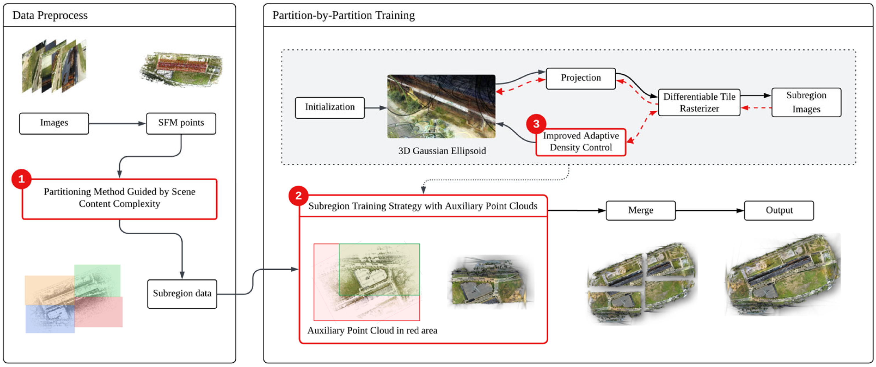
Figure 1. Overview of the proposed method. In ➁, the red area contains auxiliary point clouds, which are not involved in the densification process, whereas the green area contains point clouds that undergo densification.
Remotesensing 17 03868 g001
Figure 2. Subregion training with auxiliary point clouds. (a) Sparse points in the current subregion (green) and in the adjacent subregion (red) within the overlapping area. (b) Initialize Gaussians both in green and red areas. (c) Partition-wise optimization, where only local Gaussians are densified and fully updated, while Gaussians in the red area keep fixed geometry and only provide additional supervision across the subregion boundary. (d) Final Gaussians of the optimized subregion after cropping operation, where Gaussians in the red area serve as temporary supervision during optimization without increasing the number of Gaussians.
Remotesensing 17 03868 g002
Figure 3. Overview of the improved adaptive density control workflow. The gray-shaded areas denote the components enhanced in this work.
Remotesensing 17 03868 g003
Figure 4. Coverage analysis for Gaussians near the image periphery.
Remotesensing 17 03868 g004
Figure 5. Overview of the computational workflow for adaptive density control based on pixel-weight scaling. The direction of the arrows in the figure indicates the direction of the gradient, with the length of the arrows representing the magnitude of the gradient. The numbers in the small squares represent the count index of the Gaussian primitives covering the corresponding pixels.
Remotesensing 17 03868 g005
Figure 6. Overview of adaptive multiscale training scheduling strategy.
Remotesensing 17 03868 g006
Figure 7. Camera layout of the datasets used in the experiments.
Remotesensing 17 03868 g007aRemotesensing 17 03868 g007b
Figure 8. Statistic comparisons of our method and other 3DGS-based methods. (a–c) represent the data statistics for the three metrics: PNSR, SSIM, and LPIPS, across different methods. 3DGS performs moderately across all metrics, while the method proposed in this paper achieves optimal or near-optimal performance in all three metrics, with overall performance comparable to the multi-GPU 3DGS method.
Remotesensing 17 03868 g008
Figure 9. Results comparison of full scene. The red box in the “Ground Truth” highlights the zoomed-in region.
Remotesensing 17 03868 g009
Figure 10. Hardware-consumption comparison of 3DGS methods which support single-GPU deployment. (a) Comparison of optimization time, compared to 3DGS†, the method proposed in this paper significantly improves training efficiency, reducing optimization time by up to 71%. (b) Comparison of allocated memory, all three methods use less than 12 GB of memory.
Remotesensing 17 03868 g010
Figure 11. Comparison of per-block optimization time and total optimization time of different methods on an aerial photogrammetry dataset.
Remotesensing 17 03868 g011
Figure 12. The visualization of scene partition result.
Remotesensing 17 03868 g012
Figure 13. Comparison of results before and after applying the improved Adaptive Density Control method.
Remotesensing 17 03868 g013
Table 1. Comparison of representative large-scale 3DGS frameworks.
MethodPartitioningSupervision/Boundary HandlingDensity/Scale Control
VastGaussianCamera-position-based grid partitioning on the ground plane;
each cell contains a similar number of training views.
Airspace-aware visibility-based camera selection and coverage-based SfM point selection to enrich supervision and reduce floaters.Original 3DGS densification/pruning within each cell;
no frequency-guided multi-scale training is reported.
CityGaussianUniform grid partitioning applied to a contracted global Gaussian prior in a bounded cubic space.Coarse global Gaussian model used as initialization;
SSIM-based view assignment combined with camera location to select training views for each block.
Decomposed-gradient-based densification;
block-wise level-of-detail representation mainly for efficient rendering.
BlockGaussianRecursive bisection of the ground-plane sparse SfM point cloud, yielding content-aware blocks of varying size.Auxiliary point clouds together with visibility-aware block optimization and a pseudo-view geometry constraint to mitigate supervision mismatch and boundary artifacts.Original 3DGS densification; no explicit multi-scale training schedule is introduced.
The
proposed work
KD-tree subdivision on the ground plane guided by SfM point density, with joint control of point count and view–region correlation to balance computational load across blocks.Overlapping regions and non-densifying auxiliary Gaussians to preserve cross-block geometric and photometric consistency while controlling model growth.Pixel-weighted adaptive density control and a frequency-aware multi-scale training strategy over image resolution and Gaussian budget.
Table 2. Performance comparison of two ADC strategies on the Mill 19 dataset.
MethodNumber of GaussiansTraining Time (s)
Original ADC9,190,7274362.28
ADC Based on Pixel-Weight Scaling15,834,6766320.63
Table 3. Basic attributes of datasets. The unit of the cover area for MatrixCity-S and Pix4D-1469 is square kilometers, while the unit for the other datasets is square meters.
DatasetsTraining ImagesTesting ImagesResolution (px)Average Size (MB)Cover Area
Rubble1657214608 × 34566206 × 248
Building1920204608 × 34566262 × 438
Residence2561215472 × 36482.5291 × 491
Sci-Art2998214864 × 36482373 × 317
MatrixCity-S63627411920 × 108042.7
Pix4D-14691454155958 × 3972161.2
Table 4. Graphics card performance comparison.
GPUFP32 Compute Performance
(TFLOPS)
Tensor Performance 1
(FP16)
AI TOPS 2
(INT8)
Performance Comparison
(baseline: RTX 3090)
RTX 309035.6711421×
RTX 507048.797.5389.91.4×
RTX 409082.682.66612.3×
RTX 5090104.883833522.9×
1 Tensor performance refers to the performance achieved through computations using Tensor Cores. 2 AI TOPS represents the number of integer operations executed per second.
Table 5. Training configs and implementation details of all 3DGS-based comparison methods.
MethodGPUDensification ConfigurationIteration Budget & ScheduleDown-Sampling
3DGSSingle
RTX 3090
Original gradient-based ADC; default densification configurationDefault scheduleDefault config
CityGSMulti-GPUNative CityGaussian training settingsDefault scheduleDefault config
DOGSMulti-GPUOriginal DOGS densification & distributed schemeDefault scheduleDefault config
3DGS†Single
RTX 3090
Original gradient-based ADC; densification iterations [1000, 17,500]; cycles: 150/400/50035,0000.25
BlockGaussianSingle
RTX 3090
Densification iterations [1000, 20,000]; cycle = 200 (750 for Pix4D-1469 to avoid OOM)40,0000.25
OursSingle
RTX 3090
Pixel-weighted ADC with scaling; adaptive multi-scale scheduling; densification [1000, 17,500]; cycles: 150/400/50035,0000.25
Note: All re-implemented baselines (3DGS, 3DGS†, BlockGaussian, and our method) were trained on the same workstation (Intel Xeon 6620R CPU, 64 GB RAM), using identical train/test splits and the same loss function (L1 + SSIM with λ = 0.2), ensuring fair comparison across methods. Methods that cannot be executed on a single 24 GB GPU under their official configurations (CityGaussian, and DOGS) were not re-trained. Instead, we report the quantitative results directly from their respective publications to preserve consistency with their native multi-GPU training setups.
Table 6. Quantitative comparisons of our method and others on the Mill-19 dataset. The best and second-best results are highlighted in bold and underlined, respectively.
ScenesBuildingRubble
PSNR↑SSIM↑LPIPS↓Train↓PSNR↑SSIM↑LPIPS↓Train↓
Mega-NeRF20.920.5470.45419 h 49 min24.060.5530.50830 h 48 min
Switch-NeRF [51]21.540.5790.39724 h 46 min24.310.5620.47838 h 30 min
3DGS19.670.6680.34201 h 29 min24.750.7680.27501 h 35 min
DOGS22.730.7590.20403 h 51 min25.780.7650.25702 h 25 min
CityGS21.550.7780.246-25.770.8130.228-
Ours22.120.7660.23701 h 31 min26.350.8030.23401 h 26 min
Table 7. Quantitative comparisons of our method and others on the UrbanScene3D dataset. The best and second-best results are highlighted in bold and underlined, respectively.
ScenesResidenceSci-Art
PSNR↑SSIM↑LPIPS↓Train↓PSNR↑SSIM↑LPIPS↓Train↓
Mega-NeRF22.080.6280.40127 h 20 min25.600.7700.31227 h 39 min
Switch-NeRF22.570.6540.35235 h 11 min26.510.7950.27134 h 34 min
3DGS21.280.7820.23901 h 42 min21.430.8280.23900 h 53 min
DOGS21.940.7400.24404 h 33 min24.420.8040.21904 h 23 min
CityGS22.000.8130.211-21.390.8370.230-
Ours22.210.7990.21401 h 49 min22.760.8200.23603 h 11 min
Table 8. Quantitative comparisons of our method and others on the MatrixCity-S. The best and second-best results are highlighted in bold and underlined, respectively.
ScenesMatrixCity-S
PSNR↑SSIM↑LPIPS↓Train↓
3DGSOOM
DOGS28.580.8470.21906 h 34min
CityGS27.460.8650.204-
Ours28.990.8950.13802 h 41 min
Table 9. Performance comparison of 3DGS methods that support single-GPU deployment on four datasets. The best and second-best results are highlighted in bold and underlined, respectively.
MethodBuildingRubbleResidenceSci-Art
PSNRSSIMLPIPS#GS *PSNRSSIMLPIPS#GSPSNRSSIMLPIPS#GSPSNRSSIMLPIPS#GS
BlockGaussian22.080.7620.23713.4525.770.7900.23910.2022.460.8030.2119.6322.440.8140.2314.63
3DGS†22.170.7630.24017.5126.420.8090.22514.4722.010.7980.21415.5622.680.8220.2189.64
Ours22.120.7660.23718.5526.350.8030.23411.7922.210.7990.21414.6222.760.8200.2368.19
* #GS denotes the number of final 3D Gaussian points (106).
Table 10. Performance comparison of 3DGS methods that support single-GPU deployment on MatrixCity-S dataset. The best and second-best results are highlighted in bold and underlined, respectively.
MethodMatrixCity-S
PSNRSSIMLPIPS#GS
BlockGaussian29.130.9000.13119.15
3DGS†28.540.8920.14025.14
Ours28.990.8950.13828.80
Table 11. Quantitative comparison results of aerial photogrammetry data. The best and second-best results are highlighted in bold and underlined, respectively.
DatasetMethodPSNRSSIMLPIPS#GS *Opt. Time (min)Mem (GB)
Pix4D-1469BlockGaussianOOM39.9959510.606
3DGS†23.720.6710.36821.101678.323
Ours23.710.6980.34427.341446.693
* #GS denotes the number of final 3D Gaussian points (106).
Table 12. Scene partitioning and optimization-time statistics for different datasets.
Scenes N b l o c k s N i m a g e s m e a n N i m a g e s s t d C V ( N i m a g e ) N s f m m e a n N s f m s t d C V ( N s f m ) T o p t t o t a l T o p t s t d C V ( T o p t )
Building463739.186.15%348,4706770.101.94%5141128.7110.01%
Rubble454449.989.19%396,54010,109.782.55%491252.674.29%
Residence485727.233.18%408,2458798.812.16%602578.895.24%
Sci-Art8893270.7530.32%339,382108,859.3832.08%10,384210.6116.23%
MatrixCity-S1646969.4714.81%192,5942427.131.26%933363.6410.91%
Table 13. Performance comparison of a partition-based training strategy oriented by scene-content complexity on the Building dataset. The best and second-best results are highlighted in bold and underlined, respectively. Here “☓” or “√” represents whether the component is disabled or enabled, respectively.
Scene-Content Complexity-Based PartitioningSubregion Training Based on Auxiliary Point CloudsPSNRSSIMLPIPSTrain
(s)
Mem
(GB)
☓☓19.670.6680.342531213.33
√☓21.340.7290.26155146.64
√√22.120.7660.23754348.65
Table 14. Performance comparison of the improved adaptive density control method on the Rubble dataset. The best and second-best results are highlighted in bold and underlined, respectively. Here “☓” or “√” represents whether the component is disabled or enabled, respectively.
Weight ScalingAdaptive MultiscalePSNRSSIMLPIPSTrain (s)Opt. Time Proportion
☓☓25.940.7920.28943621.00×
√☓26.370.8120.23363201.45×
☓√25.780.7850.25635290.81×
√√26.350.8030.23451651.18×
Disclaimer/Publisher’s Note: The statements, opinions and data contained in all publications are solely those of the individual author(s) and contributor(s) and not of MDPI and/or the editor(s). MDPI and/or the editor(s) disclaim responsibility for any injury to people or property resulting from any ideas, methods, instructions or products referred to in the content.