Article

Improving Satellite-Derived Bathymetry in Complex Coastal Environments: A Generalised Linear Model and Multi-Temporal Sentinel-2 Approach

1
Marine and Coastal Unit, Geological Survey Ireland, A94 N2R6 Dublin, Ireland
2
Alfred Wegener Institute Helmholtz Center for Polar and Marine Research, 27568 Bremerhaven, Germany
3
Faculty of Geosciences, University of Bremen, 28359 Bremen, Germany
4
Oceanographic Centre of A Coruña, Instituto Español de Oceanografía (IEO-CSIC), 15001 A Coruña, Spain
5
UCD School of Geography, UCD Earth Institute, University College Dublin, D04 V1W8 Dublin, Ireland
*
Author to whom correspondence should be addressed.
Remote Sens. 2025, 17(23), 3834; https://doi.org/10.3390/rs17233834
Submission received: 15 July 2025 / Revised: 31 October 2025 / Accepted: 10 November 2025 / Published: 27 November 2025

Highlights

What are the main findings?
  • Demonstrates that combining a multi-image with Generalised Linear Model (GLM) workflow improves Satellite-Derived Bathymetry (SDB) accuracy in optically complex shallow waters (MAE = 0.34 m).
  • Evaluates the suitable number and timing of satellite images required for an effective multi-image SDB approach.
What are the implications of the main findings?
  • Provides practical guidance for selecting suitable satellite imagery to ensure reliable and accurate SDB retrievals.
  • Shows the robustness and applicability of SDB in nearshore environments, enabling broader application in coastal mapping and monitoring.

Abstract

Satellite-derived bathymetry (SDB) enhances monitoring capabilities in the context of global change and provides a cost-effective alternative to traditional in situ methods. However, a significant gap remains in the accuracy of SDB at shallow water depths (0–10 m), particularly in complex coastal settings. In this study, we developed a two-step methodology to improve shallow water depth estimates using empirical models and multi-temporal Sentinel-2 satellite imagery. Ten Sentinel-2 images from a one-year period were analysed using the Lyzenga and Stumpf empirical reference models, followed by the application of an empirical generalised linear model (GLM). Composite images were created by combining pixel values across the temporal dataset and compared with individual image results within the model. The validation results confirmed that the GLM outperformed the reference empirical models. The optimal selection of multi-temporal images demonstrated superior performance compared to single-image regression, achieving a 42% reduction in RMSE and a minimum MAE of 0.34 m. Furthermore, enhanced outlier identification within the multi-temporal analysis reduces local anomalies and enables further improvements in accuracy. These findings underscore the enhanced capability of GLM and multi-temporal images for improving the accuracy of SDB, with a relevant impact on many coastal monitoring applications and potential for scalable implementation in other regions.

1. Introduction

Coastal regions are highly variable and influenced by human activities (e.g., seafloor structures, fishing, and anchoring) and natural phenomena (e.g., storms, erosion, and flooding), with impacts potentially magnified by climate change [1,2]. Regularly updated and detailed data on seabed morphology and water levels are vital for commercial, scientific, and societal objectives and are deemed essential for human well-being [3]. Bathymetric information is crucial for assessing geological hazards [4], understanding marine habitats [5], tracking seafloor changes over time [6], and modelling future changes [7]. These frequent and substantial alterations in coastal zones necessitate effective monitoring techniques that continuously update bathymetric and seafloor topographic data. Accurate seafloor data are also imperative to meet the objective of protecting at least 30% of the world’s oceans by 2030 (Target 3 of the Kunming-Montreal Global Biodiversity Framework) [8] and to support Sustainable Development Goal 14-Life Below Water under the 2030 Agenda for Sustainable Development [3]. Seawater depth information is commonly collected using single- or multibeam echo sounders. However, some shallow coastal areas remain unmapped because of navigational hazards, time-consuming operations, inaccessible protected areas, and cost management issues [9].
Alternative methods for deriving bathymetric data, such as satellite images and remotely operated vehicles, have been used to cover the remaining shallow areas and produce complete bathymetric maps [10,11]. The use of satellite-derived bathymetry (SDB) has increased considerably in the last decade, particularly following the launch of the Sentinel-2 mission under the Copernicus program [12]. The technical characteristics of Sentinel-2 are considered an improvement over other optical sensors onboard satellites, such as Landsat and SPOT, for SDB because of the increased number of bands and their higher spatial resolution (10 m). This European Earth observation mission is formed by two twin satellites, Sentinel-2A (launched in 2015) and Sentinel-2B (launched in 2017), which follow the same sun-synchronous orbit and are phased 180° apart. This configuration allows for a revisit time of only five days at the equator and 2/3 days at higher latitudes. In September 2024, Sentinel-2C was launched to replace Sentinel-2A and guarantee the lifespan and data quality of the mission, forming a constellation of three operational satellites and enhancing the observation capabilities of the mission.
The estimation of shallow water depths using optical satellite images, such as Sentinel-2, follows two main approaches: a statistical approach, which includes empirical algorithms, and a physically based radiative transfer approach [13]. While empirical algorithms require in situ bathymetric data to derive coefficients through a regression fit, physics-based models analyse the attenuation of electromagnetic waves, considering water column constituents and sea bottom type, without the requirement of in situ bathymetric information [14]. Each method has its own advantages and disadvantages, which are determined mainly by the resources available for each study. Because of their methodological simplicity, empirical models, such as the linear band model from [15] and the band ratio model from [16], are the two most common models found in the literature [13]. However, despite their methodological advantages, these methods are highly influenced by the bottom type and water column constituents, such as turbidity [17]. Therefore, some studies have focused on enhancing the performance of these algorithms by adjusting the nonlinearity between water depth and reflectance values. For example, some authors have used statistical approaches, such as generalised linear models [18,19] or spatial prediction models [20,21], to determine the optimised relationships between reflectance bands and depth values. More advanced techniques, such as machine learning models e.g., [22,23], have also been used for estimating SDB; however, their data requirements and computational complexity are not always an advantage for users e.g., [24,25].
Image selection is also a crucial step in achieving accurate results for optical SDB. To avoid using poor-quality images, most studies have assessed the suitability of images simultaneously with in situ data based on factors such as the absence of sunglint, high water transparency, and lack of swell [17,26]. In recent years, there has been increasing interest in using combinations of multi-temporal images to improve the accuracy of SDB, for example, [27,28,29,30]. However, further research is needed to optimise these methodologies because coastal environments are complex and vary significantly among coastal regions. Cloud-based platforms, such as Google Earth Engine, also offer new opportunities in SDB for analysing large numbers of images, along with powerful computational resources [31]. However, the use of statistical methods in multi-temporal analysis offers new opportunities compared to cloud-based platforms for refining the SDB algorithm in the search for optimal SDB results.
A significant gap exists in the accuracy of SDB at shallow water depths (0–10 m). Despite advancements in SDB modelling, such as data fusion [32], multi-image approaches [29], and AI methodologies [33], consistently achieving the level of accuracy required in these challenging settings remains difficult. In the context of hydrographic surveys, “accuracy” typically refers to the total vertical uncertainty (TVU) as defined by the International Hydrographic Organization (IHO) S-44 standards [34], which set internationally recognised thresholds for depth measurement quality. For example, under IHO Order 1a, the TVU at 5 m water depth is ±0.50 m (IHO, 2020). Achieving this level of precision would significantly enhance the utility of SDB in monitoring seafloor change in dynamic coastal zones. Current empirical and physics-based approaches struggle to fully account for the complex optical interactions in shallow and turbid waters [35]. This difficulty is largely attributed to changing environmental conditions and, more significantly, to the inherent optical variability in satellite imagery and pixel-to-pixel heterogeneity [36]. The combination of multiple images and empirical models that account for nonlinearity, together with the advanced technical capabilities offered by Sentinel-2 satellites, could offer new opportunities to improve SDB precision while minimising reliance on extensive user input or specialised expertise.
This study sought to develop a scalable semi-automated methodology for estimating water depth by employing optimised empirical generalised linear models (GLM) in conjunction with multi-temporal Sentinel-2 satellite imagery. The research objectives were as follows: (a) to compare the performance of the GLM with traditional satellite-derived bathymetry (SDB) empirical models, (b) to assess the accuracy of the GLM in estimating shallow water depths from Sentinel-2 images, and (c) to evaluate the efficacy of the multi-image SDB approach.

2. Methodology

2.1. Study Area

The study area of Portrane–Rush is situated approximately 25 km north of Dublin City in County Fingal, northeast Ireland. It includes two beaches, South Rush beach (Rush) and Burrow beach (Portrane), both of which are approximately 2 km long and separated by the mouth of the Rogerstown Estuary. The coastal area near the Rogerstown Estuary represents an important environmental site with Special Area of Conservation (SAC) and Special Protection Area (SPA) designations (Figure 1). This was attributed to the presence of coastal habitats, such as salt marshes and sand dunes, and species listed in Annex I/II of the EU Habitats Directive [37]. This area, with a mean tidal range of about 4 m, has attracted considerable attention in recent years because of the strong coastal erosion that threatens the dwellings near the coastline. Ref. [38] reported a coastal retreat of 0.60 m/yr ± 0.92 m, with a higher erosion in the southern part of Burrow beach and a less severe rate towards the north, in proximity to the Rogerstown estuary mouth, mainly caused by the effects of climate change, including sea level rise and coastal storms.
Compared with other fine-grained, non-estuarine coastal settings, such as broad stretches of Ireland’s Atlantic coast, the study area’s water column is more complex and less optically clear. Secchi disk measurements in proximity to the Rogerstown Estuary mouth (EPA, 2023) (station RG090, Figure 1) ranged from 1 m in May to 2 m in July 2021. Low visibility can be attributed to high chlorophyll-a concentrations, which ranged from 1.3 µg/L to 4.1 µg/L, as reported in Table 1. While no other station in our study area performed Secchi disk tests in 2021, a station east of Portrane (station DB750, Figure 1) located in deeper waters reported Secchi disk depths of 4 and 3 m in July and August 2020, respectively. Temperature and salinity are also factors to be considered in this study. While warmer water tends to have higher absorption coefficients in the infrared region of the electromagnetic spectrum [39], higher salinity levels lead to light absorption, particularly in the green and red regions of the electromagnetic spectrum [40]. These effects are particularly relevant in high-latitude regions, such as the study area, where a low solar elevation angle further influences light absorption and spectral response.

2.2. Satellite and In Situ Bathymetric Data

2.2.1. Satellite Images

Images were downloaded from the Surface Reflectance (SR) Sentinel-2 data catalogue using the Google Earth Engine platform. This dataset comprises atmospherically corrected Level-2A Bottom-Of-Atmosphere (BOA) reflectance Sentinel-2 (S2) images processed with Sen2Cor v2.12.03 [41]. A total of 144 Sentinel-2 images were available in the catalogue for 2021, corresponding to the year of bathymetric data collection. All 144 images were preliminarily screened using a single criterion by applying Lyzenga’s SDB model [42], with a threshold of R2 > 0.7. This threshold provided a reasonable balance between selecting images with a strong correlation between reflectance and depth, while retaining a sufficient number of scenes for multi-temporal analysis. No additional filtering was necessary, as the high correlation effectively excluded images affected by clouds or other unsuitable conditions. Ten images met these criteria and were selected for further analysis (Table 2). No tidal corrections were applied to the imagery. In this study, Sentinel-2 bands 2 (blue), 3 (green), and 4 (red), each with a 10 m pixel size, were used. The near-infrared band (B8) from Sentinel-2 was used to mask land in the study area using the NDWI index with a threshold of 0.

2.2.2. In Situ Bathymetric Data

In situ bathymetric data were collected under the INFOMAR program [43] between 10 November and 3 December 2021. These data were acquired using a multibeam echosounder onboard the R.V. Geo, operated by the Geological Survey Ireland (GSI). Bathymetry data were checked for quality using hydrographic software to meet the International Hydrographic Organization (IHO) Order 1a standards. A total of five transects, with depths between +3 m and −10 m (Lowest Astronomical Tide, LAT), were used in the analyses (Figure 2). The data were then corrected for tides and transformed into a mean sea-level (MSL) datum. Information on tide levels was obtained from a tide gauge located at Skerries Harbour, approximately 10 km north of the study area, which is part of the Irish National Tide Gauge Network (Irish Marine Institute). Based on previous SDB studies on the Irish east coast using Sentinel-2 [17,21], we limited our analysis to the 0–10 m depth range at mean sea level (MSL). The bathymetry dataset consisted of 2431 observations collected along five north–south tracklines (labelled 1–5 from south to north), with a minimum horizontal spacing of 6 m between neighbouring points. To minimise spatial autocorrelation and ensure independent model evaluation, data from lines 1, 3, and 5 (1346 points) were used to train the empirical models, while points along lines 2 and 4 (1085 points) were reserved for validation. This stratified, trackline-based split provided comparable sample sizes for model calibration and validation and more realistically reflected the spatial heterogeneity of the study area.

2.3. SDB Empirical Models

2.3.1. Lyzenga Model

One of the most widely used empirical models was first proposed by [42] and later updated by [15,44]. This method assumes a linear relationship between the log-transformed radiance bands and known depths:
z = h 0 + i = 1 N h i X i
where h0 and hi are the slope and coefficients derived using linear regression, respectively, and N denotes the total number of bands used. In [42], Xi is defined as
X i = l n ( R w λ i R λ i )
where Rw is the above-surface radiance for band λi, and R is the average deep-water radiance, including atmospheric and sun glint corrections.
In Equation (2), the water optical properties are assumed to be uniform, and atmospheric scattering and surface reflection are considered the main contributors to deep-water signals. Nevertheless, as described in Section 2.2, the waters of the study area can present high turbidity patterns, which can result in high reflectance signals that may be incorrectly classified as shallower waters [17,45]. Therefore, in this study, the deep-water correction term was neglected from Equation (2), and the log-transformed radiance and X, as described in [46]:
X i = l n ( n R w λ i )
where n is a constant that ensures a positive value for the logarithmic function under any given condition. In this study, n was set to 1000. In addition, we followed the literature convention and used the blue (490 nm), green (560 nm), and red (665 nm) bands. Thus, Lyzenga’s model can be expressed as follows:
z = h 0 + h b X b + h g X g + h r X r
where Xb, Xg, and Xr are the reflectance values for the three bands, and h0, hb, hg, and hr are the constants and coefficients of the independent variables, respectively.

2.3.2. Stumpf Model

Ref. [16] proposed a different approach to SDB, in which the estimated depth was obtained from a linear relationship with the ratio of log-transformed reflectance bands:
z = m 1 l n ( n R w λ i ) l n ( n R w λ j ) m 0
where m1 and m0 are the slope and y-intercept derived by linear regression, respectively, and n is a constant that takes the same value as in Equation (3) (n = 1000) for consistency. As in Lyzenga’s formula, Rw is the above-surface radiance for the high λi and low λj absorption bands.
Stumpf’s model assumes that the bottom albedo plays a significant role in the reflectance band values, but that such changes affect both bands similarly. Nevertheless, because a difference in band reflectance is always observed, as the depth increases, the radiance of the high-absorption band decreases faster than that of the low-absorption band. In Stumpf’s model, only two bands are selected, and the ratio is given in Equation (5). In this study, blue (490 nm) and green (560 nm) bands were used for analysis. This selection was made considering previous studies conducted close to the study area [17] and corresponded to shorter wavelengths with higher penetration into the water column.

2.3.3. Generalised Linear Model (GLM)

In this study, the GLM included the blue (490 nm), green (560 nm), and red (665 nm) log-transformed bands of Sentinel-2, adding three log-transformed interaction terms: blue*green, blue*red, and green*red. This can be written as follows:
z = h 0 + h b X b + h g X g + h r X r + h b g X b X g + h b r X b X r + h g r X g X r
where Xi and h0, hb, hg, and hr are the same as in Equation (1), and hbg, hbr, and hgr are the coefficients of the interaction terms “blue*green”, “blue*red”, and “green*red”, respectively.
To assess multicollinearity within our regression models, we employed the Variance Inflation Factor (VIF) as a collinearity diagnostic tool [47]. This test helps determine the extent to which multicollinearity affects the model. The VIF values show how much a variable’s variance increases because of multicollinearity. A VIF of 1 indicates no collinearity, whereas higher numbers indicate more collinearity. Values from 1 to 5 indicate collinearity, 5 to 10 indicate moderate collinearity, and >10 denote high collinearity. Our test showed VIF values from 3.9 to 36.6, with an average of 13.3, indicating moderate-to-strong collinearity. Despite collinearity, we retained the GLM with all band interactions. This decision was guided by the primary objective of predicting water depth rather than identifying causal factors within the SDB models [48,49]. Furthermore, examining band interactions has the potential to yield significant advancements.

2.4. Multi-Temporal Image Analysis

While single-image analysis applies empirical models to the reflectance values extracted from each image, multi-temporal image analysis combines two or more images to generate new composite images from which reflectance values can be extracted. The combination of images was performed by applying a reducer function (mean or median) to the reflectance of each pixel across a set of images. The reflectance value of pixel i for the composed image c can be written as
y i c = m e a n   y i 1 , y i 2 , , y i n
y i c = m e d i a n   y i 1 , y i 2 , , y i n
where yi1, …, yin are the reflectance values of pixel i for each image, 1, …, n, respectively.
The difference between the mean and median functions typically arises when the data exhibit skewness or deviate from a normal distribution. Unlike the mean, which is sensitive to outliers, the median represents the central tendency in a more robust manner. Given the limited number of suitable images in this study, both mean and median reducers were applied to evaluate and compare their performance. For this purpose, an exhaustive automated analysis of all possible image combinations was conducted, yielding 1023 combinations for 10 images. The combinations can be of any size, from one image up to all available images (10 in our case). The subsets with the lowest MAE were selected to assess the optimal number of images (see Section 2.5 for details in ranking methodology).

2.5. Model Performance Evaluation

The model was trained on the training dataset, and evaluation metrics were obtained by comparing predictions to the independent validation dataset. Model performance was evaluated using the coefficient of determination R2, the root mean square error (RMSE), along with the mean absolute error (MAE), and mean bias error (MBE), defined as
R 2 = 1 ( y i y ^ i ) 2 ( y i y ¯ ^ ) 2
R M S E = y i y ^ i 2 n
M A E = y i ŷ i n
M B E = ( 1 / n ) ( y i ^ y i )
where y i is the measured in situ depth, y ^ i is the depth estimated in the regression models, y ¯ is the mean of the measured in situ depth values, and n is the total number of observed values.
Both RMSE and MAE measure the average model prediction error; however, whereas RMSE penalises larger errors owing to the squaring of residuals, MAE represents the average magnitude of the errors, giving equal weight to all errors. These metrics were calculated by comparing predictions to the validation dataset. For MBE, negative values indicate underestimation; positive values indicate overestimation.
In addition to (7), (8), (9), and (10), we assessed model performance using a composite ranking. We calculated a weighted ranking score (WRS) for each model and combination. This metric integrates three performance criteria—R2 (goodness of fit), RMSE, and MAE—after non-dimensionalising RMSE and MAE by the analysed depth range (Dmax–Dmin), with equal weight assigned to each component. The score penalises lower R2 and higher errors, yielding a single value in which lower values indicate better overall performance see [50,51]. For each subset size (k = 1 to 10), we evaluated all image combinations and selected the combination with the lowest MAE; WRS is reported alongside as a composite indicator for comparison.
WRS = ((1 − R2) + RMSE/(Dmax − Dmin) + MAE/(Dmax − Dmin))/3
Following the recommendation of [52], we also conducted an explanatory analysis to identify outliers using the median and median absolute deviation (MAD), as these parameters are not strongly affected by extreme values, as in the case of the mean and standard deviation. Nevertheless, extreme values can often be part of the curve tendency, which may be over- or underestimated at different depth ranges. Therefore, a highly conservative threshold value of 3 was selected [53] to avoid erroneous classification of outlier points that are part of the curve. Outliers are further categorised as either “Isolated” outliers or “Persistent” outliers, depending on the number of images showing the same point as an outlier. This classification helps distinguish outliers caused by day-specific artefacts from anomalies resulting from model-based constraints.

3. Results

3.1. Comparison of SDB Models

The validation results for the three tested SDB models are presented for the ten analysed images (Table 3). Lyzenga’s R2 coefficients ranged between 0.79 and 0.89 and were, on average, 31% higher than those obtained by applying Stumpf’s model (mean 0.85 vs. 0.65), which ranged between 0.35 and 0.82. Lyzenga’s models showed lower WRS values than Stumpf’s models for all the images. Lower RMSE and MAE values were also achieved for Lyzenga’s models, with an average improvement over Stumpf’s of 0.57 m and 0.46 m, respectively. The highest accuracy scores were achieved when Lyzenga’s model was applied to image IDs 6, 7, and 8, which were obtained within the same week of July 2021. These three images had the highest R2 values (0.88–0.89) and the lowest RMSE and among the lowest MAE values of all the images. Conversely, these three images did not show consistent scores when Stumpf’s model was applied, with R2 values ranging from 0.47 to 0.75. Image ID 1 exhibited the largest variation between the two models, with an increase in the RMSE of around 1.2 m, and the coefficient of determination R2 dropped to 35% when using Stumpf’s model, which was the lowest value among all the analysed images.
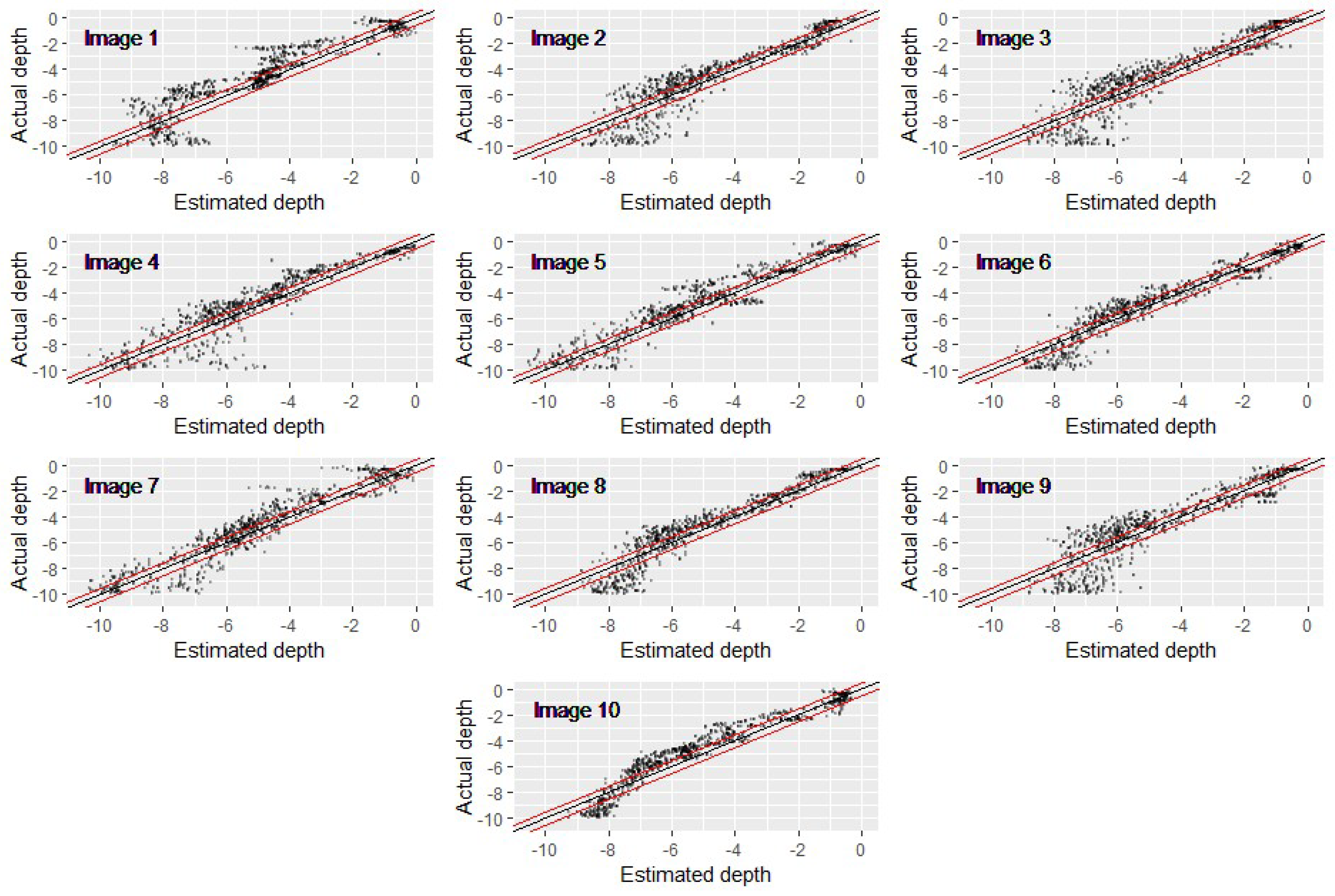
The GLM models returned better fits than the Lyzenga and Stumpf models (Figure 2). Better fits of the GLM over Lyzenga’s models were confirmed by the lower WRS values for the ten images (lower for GLM in all 10 images; ~15% mean paired reduction). Compared with Lyzenga’s model, the GLM showed an average RMSE and MAE reduction of 0.11 m across the ten images, along with a 3% increase in R2 values (from 0.85 to 0.88 on average). Within the single-image results, three high-performing GLM cases came from the same week in July (IDs 6–8). Within this July subset, the best case reached R2 = 0.92 with RMSE = 0.77 m and MAE = 0.58 m. Across all images, the highest R2 (0.92) occurred for Image ID 10, which also showed the largest improvement over Lyzenga (R2 +10%, RMSE −0.35 m, MAE −0.30 m). Across image subsets, MBE remained near zero for GLM and small for Lyzenga (typically <5% of the analysed 0–10 m depth range), indicating no meaningful systematic bias relative to RMSE/MAE (see Table 3). Considering these results, in the following sections on multi-temporal image analysis, we adopted the GLM as the primary model because of its consistently lower WRS across all images. The results of Lyzenga and Stumpf were incorporated to support and enhance our interpretation of the data.

3.2. Evaluation of Multi-Temporal Image Analysis

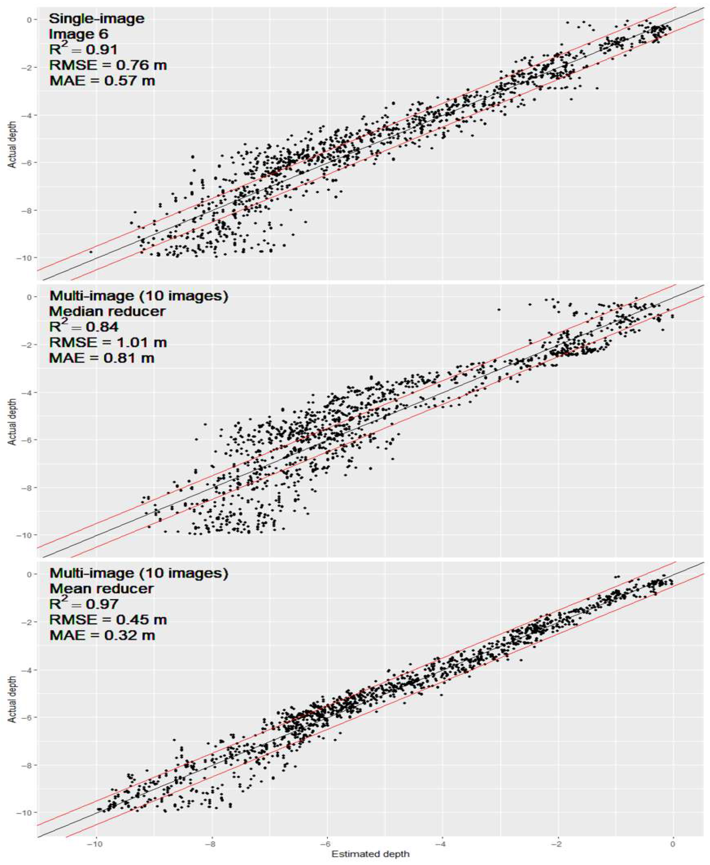
In Figure 3 and Table 4, the plots and scores of the multi-image model considering all 10 images are compared with the results of image ID 6, which is the single image with the best overall performance obtained using the GLM (Table 3): R2 of 0.92, RMSE 0.77 m, and WRS 0.072.
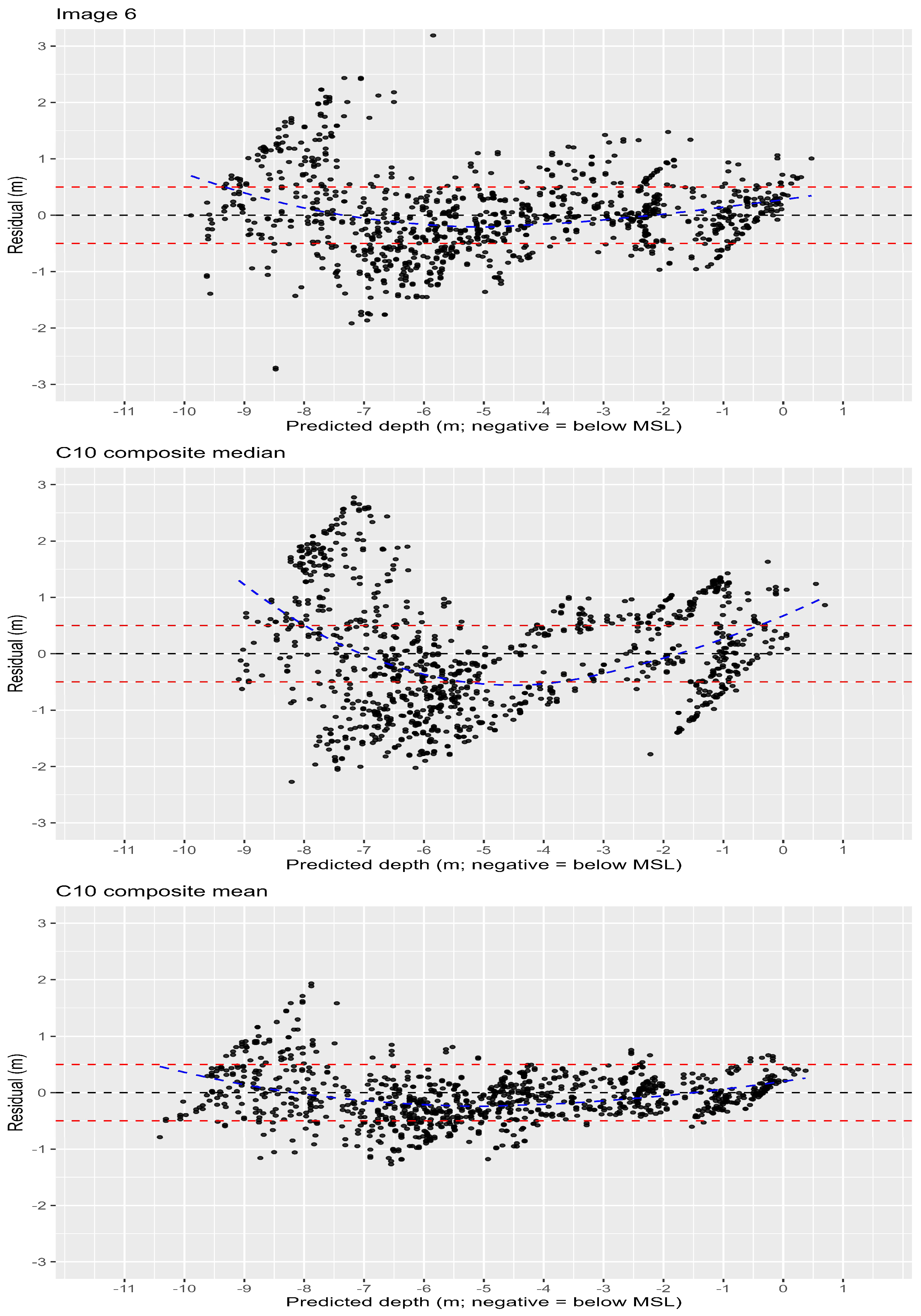
The residual plots (Figure 4) show the distribution of model errors across depth, revealing relatively consistent error margins from 0 to 6 m. Between 6 and 7 m, some irregular patterns appear, and beyond 7 m, the errors increase substantially, with a greater scatter of both over- and underpredictions. These results suggest that the effective depth limit for reliable model performance (that is, the extinction depth) can be estimated at approximately 7 m, which also corresponds to the highest observed R2. Optimal performance was achieved within the 0 to 7 m range, with markedly lower errors than the 0 to 10 m interval (R2 = 0.98, RMSE = 0.31 m, MAE = 0.24 m, WRS = 0.033).
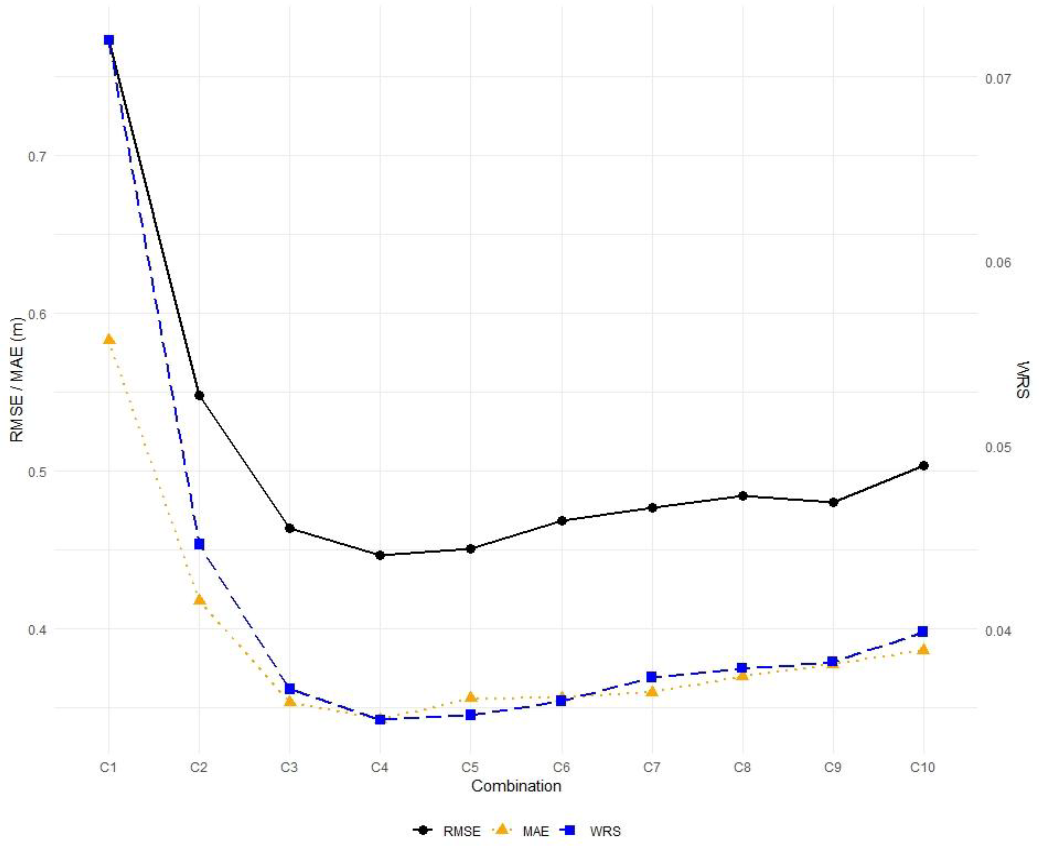
The multi-image analysis identified the best-performing image combinations for each subset size (Figure 5). For each size from one to ten images, we selected the combination with the lowest MAE. The highest-performing combination, C4 (combination 297), used four images and achieved R2 = 0.974, RMSE = 0.45 m, MAE = 0.34 m, and WRS = 0.035. Relative to the best single image (ID 6), this corresponds to an increase in R2 from 0.92 to 0.974 (5.4 percentage points) and reductions of 0.32 m in RMSE and 0.24 m in MAE. The all-image composite (C10) is not among the best performers; in the overall top-ten list (Table 5), most high-ranking combinations contain 3–8 images, with the best typically comprising 3–6 images. From C3 to C10, MAE differs by no more than 0.03 m and WRS by no more than 0.003. From C5 to C10, there is a gradual decline in performance, indicating that adding more than five images does not improve accuracy. Image ID 1 does not appear among the top-ten combinations.

3.3. Outlier Analysis

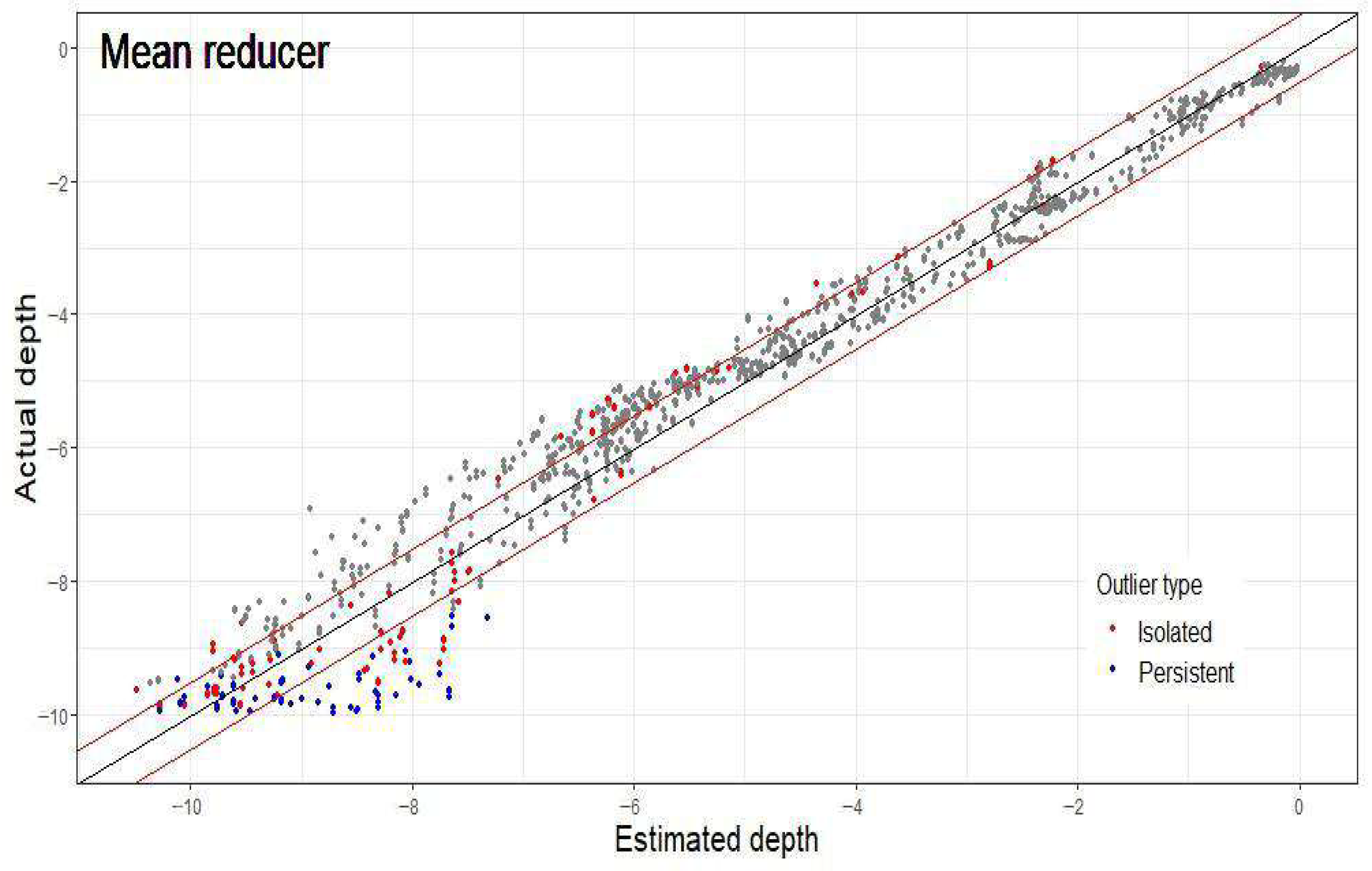
A close examination of the GLM results across the set of images showed 257 outliers identified using the MAD parameters (Section 2.5). Of the 257, 91 are categorised as “Isolated” outliers, appearing in only one image; the remaining 166 appear in more than one image and are therefore classified as “Persistent” outliers. After grouping detections by validation point across the full image set, these 166 Persistent detections correspond to 60 unique Persistent outlier points, of which 27 (45%) fall within ±0.5 m.
The lowest number of outliers was found in image ID 10, with only one Persistent outlier (Table 6). The highest number of outliers occurred in image ID 3, with 55 total outliers, 26 Isolated outliers, and 29 Persistent outliers.
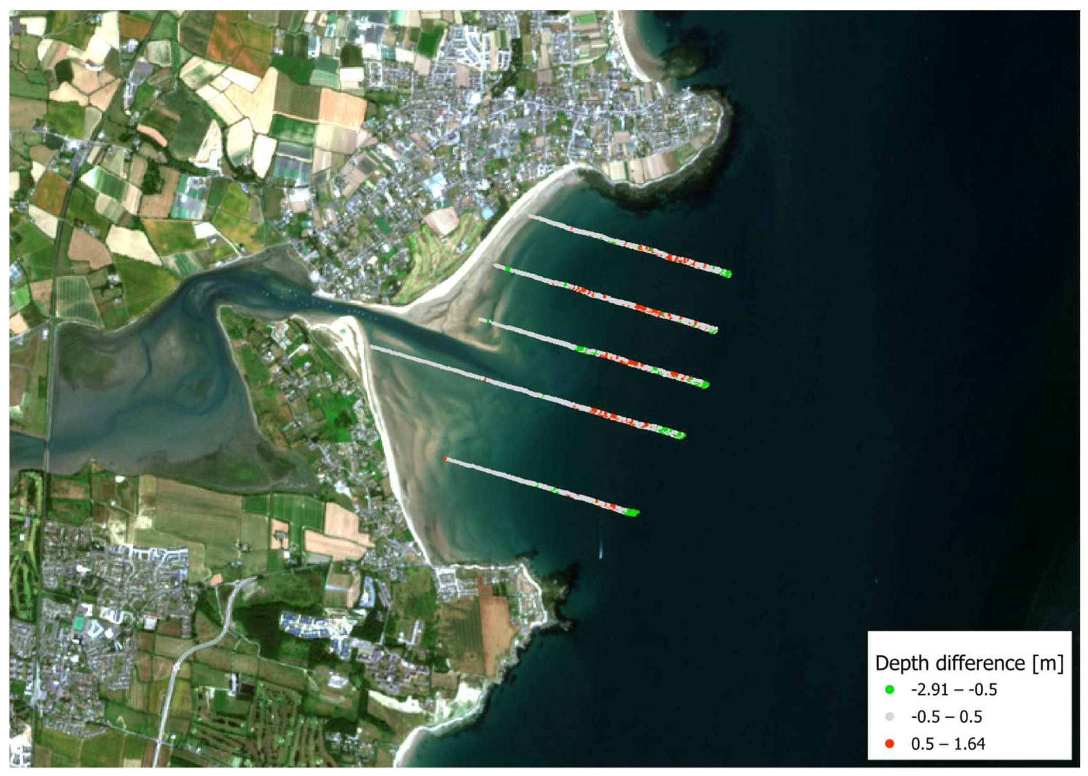
The multi-image datasets obtained through a mean reducer change the outlier distribution relative to a single image. Figure 6 shows the linear trend of the 10 combined images, resulting in 49 of the 91 Isolated outliers (54%) falling within the ±0.5 m error, while the Persistent outliers only have 27 of the 60 (45%) in the ±0.5 m error range. Almost all Persistent outliers occurred at depths greater than 7 m, whereas Isolated outliers were observed across most depth ranges (see Figure 7 for the spatial distribution of the residuals).

4. Discussion

4.1. Water Clarity and Optical Conditions

The optical properties of the North Irish Sea waters, particularly the increased turbidity near the estuary, reduce light penetration and limit the effectiveness of satellite-derived bathymetry (SDB) [54]. In this study, Secchi disk measurements ranged from 1 to 4 m (Table 1), reflecting substantial variability in water clarity across the area. The lowest Secchi disk depth (1 m) was recorded in May 2021 at station RG090, located at the mouth of the estuary, where estuarine currents further reduce visibility. In contrast, station DB750, located in deeper waters approximately 3 km south of the study area, showed Secchi disk depths of 4 m in July and 3 m in August 2020. These measurements match earlier observations of water clarity and light penetration in the region [54] and confirm that the observed Secchi disk depth range is comparable to the conditions under which successful SDB mapping has been achieved in other complex coastal waters [32,46,55].

4.2. Image Selection and Compositing Strategy

The selection of Sentinel-2 images for SDB in this study was based on an R2 threshold greater than 0.7, which is consistent with previous studies in similar settings [17]. Applying this threshold defined a suitable time window for image acquisition from April to September, corresponding to solar altitudes of at least 41°. Within this period, the most accurate results across all empirical models were obtained in June and July. These months have the highest solar altitude (about 61°, 21 June) and generally the most stable atmospheric conditions, such as less rainfall, calmer winds, and higher pressure. Within April to September, sea conditions were typically calmer in June and July, based on wave height records from the nearby M2 buoy (www.marine.ie), which would be expected to improve water column visibility and bottom-signal retrieval. Within this April to September window, single-image GLM performance was strongest in mid-July (IDs 6 to 8), and a late-September scene (ID 10) also performed strongly, achieving the highest single-image R2.
Our findings show that multi-image compositing improves SDB accuracy compared to single-image analysis, as reported in other studies [23,29,32], but only when using a mean reducer. Median compositing, as used by other authors e.g., [28,32], yielded lower accuracy in our analyses. The mean reducer outperformed the median in our case, with a limited number of images. While the exact mechanism requires further investigation, one possible explanation is that the mean makes use of all values, whereas the median downweights extremes that may still carry significant depth information. The mean-composited image produced better fits than single-image models and significantly reduced noise at all depths, particularly in the shallow depth range up to 4 m, as observed in the residual plots (Figure 4).
Across the combination rankings (Table 5; Figure 5), a consistent core is evident: images 2, 5, 6, and 8 recur in the highest-scoring subsets, with 7 and 10 frequently added thereafter. Image 1, acquired at the lowest tide and in early April, does not enter the top combinations, indicating that its acquisition conditions transfer less effectively to the remainder of the series. With respect to subset size, at least three images are needed to stabilise estimates; beyond two scenes, averaging reduces sensitivity to any single scene’s conditions. From C3 to C10, MAE varies by no more than 0.03 m, with the best case at C4 (MAE = 0.34 m, RMSE = 0.45 m). Larger sets do not yield further improvement, and performance declines slightly from C5 to C10, with changes in MAE below 0.03 m.

4.3. Depth-Dependent Error Patterns

Tide levels referenced to LAT across the ten Sentinel-2 images (Table 2) ranged from 1.03 m to 3.57 m, with a tidal range of 2.53 m and an average level of 1.95 m. Nine images were acquired at low to mid tides (1.03–2.64 m), while one image (image ID 2) was acquired at high tide (3.57 m). In the shallow depth range (0–2 m), Figure 3 shows high pixel-to-pixel variability in the single-image results, which we attribute to the strong seafloor contribution in very shallow water. This variability is primarily seafloor-driven; at 0–2 m, the seafloor signal is intrinsically tied to tide level across dates because small water-level changes alter the water column and reflectance. In the multi-image composites, the median composite shows greater scatter at 0–2 m, whereas the mean composite reduces it. This behaviour is consistent with the tide spread in Table 2 (≈2.5 m), where different acquisitions sample markedly different water-column thickness at the same locations. In contrast, mean composited image models yielded more stable estimates across this depth range, with most points remaining within ±0.5 m error margins (Figure 4).
The estimated light extinction depth in this study was determined to be between 6 and 7 m, as inferred from the GLM plots and residuals (Figure 4), and matches the findings in nearby Irish Sea coastal areas with similar water optical properties [17,56]. These influential environmental properties underscore the need for careful image selection and compositing strategies across optically complex depth intervals.

4.4. Generalised Linear Model Interpretation

We used a GLM with band terms and pairwise interactions to relate surface reflectance to depth. This is achieved by retaining band terms to improve the characterisation of depth variations under different water conditions and seafloor reflectance types [15,57]. Predictors and their interactions are often highly correlated, especially the blue and green bands under shallow-water conditions, with VIF > 5. Given this collinearity, we do not interpret individual coefficients and focus instead on predictive performance, as such collinearity is deemed acceptable for predictive purposes and does not necessarily reduce accuracy when the primary objective is forecasting rather than inference [48,58,59]. Prior work supports this view, showing that adjusting or transforming reflectance terms, even if collinear, preserves the physical light–depth relationships without biasing the model outputs [19].
Our GLM results for single-image analyses yielded lower RMSEs than traditional empirical methods, such as those described by Lyzenga and Stumpf, indicating an effective balance between flexibility and accuracy. This pattern was evident for the July images (IDs 6–8) and for Image ID 10, where GLM achieved the highest single-image R2 and the largest gains over Lyzenga. Following established hydro-optical modelling principles, retaining these terms prevents the loss of significant information that could otherwise reduce predictive effectiveness [60,61]. Importantly, previous SDB studies have observed that simple regression frameworks, such as standard linear regression and generalised linear models, require relatively modest training datasets and provide explicit coefficients that relate spectral bands to depth, which can make their results easier to interpret than those of highly flexible machine learning or additive models [48,61]. Such models can serve as an initial approach, delivering solid predictive performance with limited data and laying the groundwork for incorporating more sophisticated methods once there is a clearer understanding of image suitability and ancillary information.

4.5. Limitations and Practical Implications

Outlier detection revealed two types of deviations: Isolated outliers linked to image-specific artefacts, and Persistent outliers observed across images. The latter is more likely to represent systematic deviations from the model assumptions rather than noise. In several instances, Persistent outliers were spatially consistent with known seabed features, including a documented rock outcrop and the estuarine channel at the mouth of the Rogerstown Estuary, which exhibits complex geomorphology and variable sediment composition. This highlights the limitations of linear models in heterogeneous environments [45,46] and underscores the need for improved bottom-type classification in future SDB frameworks.
By combining a GLM with multi-image analysis, we achieved substantial error reductions across all depth intervals (Figure 5 and Figure 6). However, this study has limitations. The small number of available images restricted our ability to further improve accuracy under different environmental conditions. Moreover, although the GLM extends beyond a simple regression model by including interaction terms and a link function, it is still fundamentally based on a linear additive structure on the scale of the predictors. This means that GLMs can struggle to capture non-linear or abrupt variations in water properties, bottom type, and light attenuation, which often characterise optically complex coastal environments [62,63].
The model’s limitations were also confirmed by the behaviours of outliers: some were image-specific, while others persisted across images and spatially coincided with known seabed features such as rock outcrops and estuary channels. This suggests that some deviations are due to abrupt changes in seafloor type or geomorphological characteristics that are not adequately captured by the GLM. This highlights the limitations of linear models in heterogeneous environments and underscores the need for improved bottom-type classification in future SDB frameworks [45,46]. More flexible non-linear approaches, such as generalised additive models or machine learning, may capture these variations more fully when larger datasets and seabed type information are available. However, the simplicity and modest data requirements of GLMs remain valuable for water depth predictions in coastal areas.

4.6. Comparison with Other Studies

In this study, integrating a generalised linear model (GLM) with a four-image composite yielded errors of 0.45 m (RMSE) and 0.34 m (MAE). Within the directly comparable 0–7 m range, the GLM achieved 0.31 m (RMSE) and 0.24 m (MAE). Direct comparisons across SDB studies are indicative only, as depth range, optical setting, and metrics differ; many studies also extend to deeper limits in clearer waters, where errors typically increase with range. With that caveat, published results provide context: Sánchez-Carnero et al. [19] reported an RMSE of 0.88 m at 0–6 m using a single SPOT-5 image and a GLM; Xu et al. [22] reported RMSE 0.99 m and R2 0.91 using support vector machines with ICESat and Sentinel-2 in the Dongsha Atoll; Casal et al. [45] reported RMSE 1.00 m and R2 0.86 (to 10 m) using a model-inversion approach with single Sentinel-2 images in Dublin Bay; and Kumar et al. [64] reported RMSE 1.09 m and 0.93 m (to 15 m) using Sentinel-2 multi-scene composites with a log-ratio transformed calibrated model. Taken together, these figures indicate that, in an optically complex coastal setting and over a restricted depth range, a GLM combined with multi-image compositing can deliver errors that are at the lower end of those reported, while recognising the limits of cross-study comparisons.
The error reductions obtained in this study using a GLM and multiple images are especially beneficial for monitoring depth changes in coastal areas where traditional ship-based surveys are less practical and more expensive. In addition, its performance on optically complex waters such as the Irish Sea suggests that this simple empirical approach can provide efficient and accurate SDB solutions under a range of environmental conditions.

5. Conclusions

The increasing number of studies on SDB following the widespread availability of optical satellite data has led to advancements in methodology to achieve improved accuracy across various coastal environments. In this study, we evaluated different models and multi-image techniques to improve accuracy and reduce uncertainty, with the potential to be scaled up to other environments and source datasets.
The main findings of this study are as follows:
  • The generalised linear model (GLM) demonstrated superior performance compared with other empirical models in minimising error margins, particularly when emphasis was placed on predictive accuracy rather than isolating the effects of individual parameters.
  • The use of multiple image composites demonstrated superior performance compared to single-image analysis, contingent on the application of the mean reducer function. Moreover, the integration of multiple images effectively reduces the occurrence of outliers in single images. Composites of 3 to 8 images delivered near optimal accuracy; adding more images beyond this did not yield further improvements.
  • The application of the generalised linear model (GLM) to a composite dataset of four images resulted in overall error margins of 0.45 m for the RMSE and 0.34 m for the MAE. These error metrics were further reduced to an RMSE of 0.31 m and an MAE of 0.24 m when the analysis was restricted to the optimal water depth range of 0 to 7 m. While these error levels are broadly comparable to shallow water tolerances referenced in IHO S-44, they are most relevant to selected applications and contexts. The obtained accuracy levels are particularly significant for monitoring coastal nearshore areas, with numerous interdisciplinary applications, including the assessment of marine habitats and the prediction of coastal changes over time. Future studies should explore the integration of seabed classification techniques and artificial intelligence models to further improve predictive accuracy and account for spatial heterogeneity in optically complex environments.

Author Contributions

X.M. and T.I. contributed to the design and implementation of the research. X.M., T.I., G.C. and C.G. contributed to the analysis of the results and to the writing of the manuscript. X.M., T.I. and C.G. conceived the original and supervised the project. All authors have read and agreed to the published version of the manuscript.

Funding

C.G.’s contributions were supported by funding from the Ramón y Cajal 2023 grant RYC2023-044898-I, funded by the Spanish State Plan for Scientific and Technical Research and Innovation 2021–2023.

Data Availability Statement

The Earth Engine code developed for this study is publicly available under an open license at: https://github.com/XMV069/SDB_GLM (accessed on 9 November 2025) (https://earthengine.google.com/). All statistical analyses were performed using R (version 4.2.2) and are available upon request.

Conflicts of Interest

The authors declare no conflict of interest.

References

  1. Halpern, B.S.; Walbridge, S.; Selkoe, K.A.; Kappel, C.V.; Micheli, F.; D’Agrosa, C.; Bruno, J.F.; Casey, K.S.; Ebert, C.; Fox, H.E.; et al. A global map of human impact on marine ecosystems. Science 2008, 319, 948–952. [Google Scholar] [CrossRef]
  2. Lipiec, E.; Ruggiero, P.; Mills, A.; Serafin, K.A.; Bolte, J.; Corcoran, P.; Walczak, J.; Tillmann, P.; O’Neill, S.M.; Goupee, J. A multi-objective evaluation of coastal protection alternatives under extreme sea level scenarios. J. Coast. Res. 2018, 34, 1196–1208. [Google Scholar] [CrossRef]
  3. Wölfl, A.-C.; Snaith, H.; Amirebrahimi, S.; Devey, C.W.; Dorschel, B.; Ferrini, V.; Huvenne, V.A.I.; Jakobsson, M.; Jencks, J.; Johnston, G.; et al. Seafloor mapping—The challenge of a truly global ocean bathymetry. Front. Mar. Sci. 2019, 6, 283. [Google Scholar] [CrossRef]
  4. Ridente, D.; Martorelli, E.; Bosman, A.; Chiocci, F.L. High-resolution morpho-bathymetry of the Messina Strait (South-ern Italy): New insights on the 1908 earthquake and tsunami. Geomorphology 2014, 208, 149–159. [Google Scholar] [CrossRef]
  5. Hedley, J.D.; Roelfsema, C.; Brando, V.; Giardino, C.; Kutser, T.; Phinn, S.; Mumby, P.J.; Barrilero, O.; Laporte, J.; Koetz, B. Coral reef applications of Sentinel-2: Coverage, characteristics, bathymetry and benthic mapping with comparison to Landsat 8. Remote Sens. Environ. 2018, 216, 598–614. [Google Scholar] [CrossRef]
  6. Mielck, F.; Hass, H.C.; Michaelis, R. Morphological changes due to marine aggregate extraction for beach replenishment in the German Bight (SE North Sea). Geo-Mar. Lett. 2019, 39, 47–58. [Google Scholar] [CrossRef]
  7. Barnard, P.L.; Erikson, L.H.; Foxgrover, A.C. Dynamic flood modeling essential to assess the coastal impacts of climate change. Sci. Rep. 2019, 9, 4309. [Google Scholar] [CrossRef]
  8. Convention on Biological Diversity. Kunming-Montreal Global Biodiversity Framework: Target 3. United Nations Environment Programme. 2022. Available online: https://www.cbd.int/gbf/targets/3/ (accessed on 9 November 2025).
  9. Guinan, J.; McKeon, C.; O’Keeffe, E.; Monteys, X.; Sacchetti, F.; Coughlan, M.; Nic Aonghusa, C. INFOMAR data supports offshore energy development and marine spatial planning in the Irish offshore via the EMODnet Geology Portal. Q. J. Eng. Geol. Hydrogeol. 2021, 54, qjegh2020-033. [Google Scholar] [CrossRef]
  10. Daniell, J.J. The Combination of Soundings and Remotely Sensed Bathymetry in the GEBCO Grid; GEBCO Science Day Proceedings: Lima, Peru, 2010; 15p, Available online: https://www.gebco.net (accessed on 9 November 2025).
  11. Lebrec, U.; Paumard, V.; O’Leary, M.J.; Lang, S.C. Towards a high-resolution global seabed sediment and rock type map: The Sand, Silt, and Rock (SSR) database. Earth Syst. Sci. Data 2021, 13, 5191–5212. [Google Scholar] [CrossRef]
  12. European Space Agency (ESA). Copernicus. 2023. Available online: https://sentiwiki.copernicus.eu/web/s2-mission (accessed on 9 November 2025).
  13. Duplančić Leder, T.; Baui, M.; Leder, N.; Gili, F. Optical satellite derived bathymetry: An overview and WoS and Scopus bibliometric analysis. Remote Sens. 2023, 15, 1294. [Google Scholar] [CrossRef]
  14. Hedley, J.; Roelfsema, C.; Phinn, S.R. Efficient radiative transfer model inversion for remote sensing applications. Remote Sens. Environ. 2009, 113, 2527–2532. [Google Scholar] [CrossRef]
  15. Lyzenga, D.R. Shallow-water bathymetry using combined LiDAR and passive multispectral scanner data. Int. J. Remote Sens. 1985, 6, 115–125. [Google Scholar] [CrossRef]
  16. Stumpf, R.P.; Holderied, K.; Sinclair, M. Determination of water depth with high-resolution satellite imagery over variable bottom types. Limnol. Oceanogr. 2003, 48, 547–556. [Google Scholar] [CrossRef]
  17. Casal, G.; Monteys, X.; Hedley, J.; Harris, P.; Cahalane, C.; McCarthy, T. Assessment of empirical algorithms for bathymetry extraction using Sentinel-2 data. Int. J. Remote Sens. 2019, 40, 2855–2879. [Google Scholar] [CrossRef]
  18. Vojinovic, Z.; Abebe, Y.A.; Ranasinghe, R.; Vacher, A.; Martens, P.; Mandl, D.J.; Frye, S.W.; van Ettinger, E.; de Zeeuw, R. A machine learning approach for estimation of shallow water depths from optical satellite images and sonar measurements. J. Hydroinform. 2013, 15, 1408–1424. [Google Scholar] [CrossRef]
  19. Sánchez-Carnero, N.; Ojeda-Zújar, J.; Rodríguez-Pérez, D.; Márquez-Pérez, J. Assessment of different models for bathymetry calculation using SPOT multispectral images in a high-turbidity area. Int. J. Remote Sens. 2014, 35, 493–514. [Google Scholar] [CrossRef]
  20. Chybicki, A. Three-dimensional geographically weighted inverse regression (3GWR) model for satellite-derived bathymetry using Sentinel-2 observations. Mar. Geod. 2017, 41, 1–23. [Google Scholar] [CrossRef]
  21. Casal, G.; Harris, P.; Monteys, X.; Hedley, J.; Cahalane, C.; McCarthy, T. Understanding satellite-derived bathymetry using Sentinel-2 imagery and spatial prediction models. GIScience Remote Sens. 2020, 57, 271–286. [Google Scholar] [CrossRef]
  22. Xu, N.; Wang, L.; Zhang, H.S.; Tang, S.; Mo, F.; Ma, X. Machine learning based estimation of coastal bathymetry from ICESat-2 and Sentinel-2. IEEE J. Sel. Top. Appl. Earth Obs. Remote Sens. 2024, 14, 1748–1754. [Google Scholar] [CrossRef]
  23. Mudiyanselage, S.S.J.D.; Abd-Elrahman, A.; Wilkinson, B.; Lecours, V. Multi-temporal satellite derived bathymetry using Sentinel-2 and machine learning. GIScience Remote Sens. 2022, 59, 1143–1158. [Google Scholar] [CrossRef]
  24. Al Najar, M.; Thoumyre, G.; Bergsma, E.W.J.; Almar, R.; Benshila, R.; Wilson, D.G. Satellite derived bathymetry using deep learning. Mach. Learn. 2023, 112, 1107–1130. [Google Scholar] [CrossRef]
  25. Susa, T. Satellite derived bathymetry with Sentinel-2 imagery: Comparing traditional techniques with advanced methods and machine learning ensemble models. Mar. Geod. 2022, 45, 435–461. [Google Scholar] [CrossRef]
  26. Evagorou, E.; Argyriou, A.; Papadopoulos, N.; Mettas, C.; Alexandrakis, G.; Hadjimitsis, D. Evaluation of satellite-derived bathymetry from high and medium-resolution sensors using empirical methods. Remote Sens. 2022, 14, 772. [Google Scholar] [CrossRef]
  27. Ilori, C.O.; Knudby, A. An approach to minimize atmospheric correction error and improve physics-based satellite-derived bathymetry in a coastal environment. Remote Sens. 2020, 12, 2752. [Google Scholar] [CrossRef]
  28. Xu, N.; Ma, Y.; Liu, Z.; Yang, B.; Yang, F.; Wang, X.H.; Li, S. Deriving highly accurate shallow water bathymetry from Sentinel-2 and ICESat-2 datasets by a multitemporal stacking method. IEEE J. Sel. Top. Appl. Earth Obs. Remote Sens. 2021, 14, 6677–6685. [Google Scholar] [CrossRef]
  29. Viaña-Borja, S.P.; Fernández-Mora, A.; Stumpf, R.P.; Navarro, G.; Caballero, I. Semi-automated bathymetry using Sentinel-2 for coastal monitoring in the Western Mediterranean. Int. J. Appl. Earth Obs. Geoinf. 2023, 120, 103328. [Google Scholar] [CrossRef]
  30. Lowell, K.; Hermann, J. Accuracy of Bathymetric Depth Change and Change Rate Estimations in Shallow Waters Based on Landsat 7 and Landsat 8 Data. J. Mar. Sci. Eng. 2024, 12, 1401. [Google Scholar] [CrossRef]
  31. Traganos, D.; Poursanidis, D.; Aggarwal, B.; Chrysoulakis, N.; Reinartz, P. Estimating satellite-derived bathymetry (SDB) with the google earth engine and sentinel-2. Remote Sens. 2018, 10, 859. [Google Scholar] [CrossRef]
  32. Sagawa, T.; Yamashita, Y.; Okumura, T.; Yamanokuchi, T. Satellite derived bathymetry using machine learning and multi-temporal satellite images. Remote Sens. 2019, 11, 1155. [Google Scholar] [CrossRef]
  33. Saeidi, V.; Seydi, S.T.; Kalantar, B.; Ueda, N.; Tajfirooz, B.; Shabani, F. Water depth estimation from Sentinel-2 imagery using advanced machine learning methods and explainable artificial intelligence. Geomat. Nat. Hazards Risk 2023, 14, 2225691. [Google Scholar] [CrossRef]
  34. IHO S-44; IHO Standards for Hydrographic Surveys, Edition 6.0.0. International Hydrographic Organization (IHO): Monte Carlo, Monaco, 2020. [CrossRef]
  35. Caballero, I.; Stumpf, R.P. Atmospheric correction for satellite-derived bathymetry in the Caribbean waters: From a single image to multi-temporal approaches using Sentinel-2A/B. Opt. Express 2020, 28, 11742–11766. [Google Scholar] [CrossRef] [PubMed]
  36. Cahalane, C.; Magee, A.; Monteys, X.; Casal, G.; Hanafin, J.; Harris, P. A comparison of Landsat 8, RapidEye and Pleiades products for improving empirical predictions of satellite-derived bathymetry. Remote Sens. Environ. 2019, 233, 111414. [Google Scholar] [CrossRef] [PubMed]
  37. European Commission, DG-ENV. Interpretation Manual of European Union Habitats, Version EUR 28. 2013. Available online: https://circabc.europa.eu/ui/group/3f466d71-92a7-49eb-9c63-6cb0fadf29dc/library/37d9e6d9-b7de-42ce-b789-622e9741b68f/details (accessed on 9 November 2025).
  38. Calder, K. Rogerstown Coastal Flood Erosion Risk Management Study Stage 1: Coastal Flood and Erosion Risk Assessment; RPS Ireland Ltd.: Belfast, UK, 2020. [Google Scholar]
  39. Pegau, W.; Gray, D.; Zaneveld, J. Absorption and attenuation of visible and near-infrared light in water: Dependence on temperature and salinity. Appl. Opt. 1997, 36, 6035–6046. [Google Scholar] [CrossRef] [PubMed]
  40. Sullivan, J.M.; Twardowski, M.S.; Zaneveld, J.R.V.; Moore, C.M.; Barnard, A.H.; Donaghay, P.L.; Rhoades, B. Hyperspectral temperature and salinity dependencies of absorption by water and heavy water in the 400–750 nm spectral range. Appl. Opt. 2006, 45, 5294–5309. [Google Scholar] [CrossRef]
  41. Main-Knorn, M.; Pflug, B.; Louis, J.; Debaecker, V.; Müller-Wilm, U.; Gascon, F. Sen2Cor for Sentinel-2. In Image and Signal Processing for Remote Sensing XXIII; SPIE: Bellingham, WA, USA, 2017; Volume 10427, p. 1042704. [Google Scholar] [CrossRef]
  42. Lyzenga, D.R. Passive remote sensing techniques for mapping water depth and bottom features. Appl. Opt. 1978, 17, 379–383. [Google Scholar] [CrossRef]
  43. O’Toole, R.; Judge, M.; Sacchetti, F.; Furey, T.; Mac Craith, M.; Monteys, X. Seabed and habitat mapping in Irish waters: INFOMAR and beyond. Geol. Soc. London Spec. Publ. 2022, 505, 71–96. [Google Scholar] [CrossRef]
  44. Lyzenga, D.R.; Malinas, N.P.; Tanis, F.J. Multispectral bathymetry using a simple physically based algorithm. IEEE Trans. Geosci. Remote Sens. 2006, 44, 2251–2259. [Google Scholar] [CrossRef]
  45. Casal, G.; Hedley, J.D.; Monteys, X.; Harris, P.; Cahalane, C.; McCarthy, T. Satellite-derived bathymetry in optically complex waters using a model inversion approach and Sentinel-2 data. Estuar. Coast. Shelf Sci. 2020, 241, 106814. [Google Scholar] [CrossRef]
  46. Bramante, J.F.; Raju, D.K.; Sin, T.M. Multispectral derivation of bathymetry in Singapore’s shallow, turbid waters. Int. J. Remote Sens. 2013, 34, 2070–2088. [Google Scholar] [CrossRef]
  47. Kim, J.H. Multicollinearity and misleading statistical results. Korean J. Anesthesiol. 2019, 72, 558–569. [Google Scholar] [CrossRef]
  48. James, G.; Witten, D.; Hastie, T.; Tibshirani, R. An Introduction to Statistical Learning: With Applications in R, 2nd ed.; Springer: Berlin/Heidelberg, Germany, 2021; pp. 367–402. [Google Scholar]
  49. Graham, M.H. Confronting multicollinearity in ecological multiple regression. Ecology 2003, 84, 2809–2815. [Google Scholar] [CrossRef]
  50. Willmott, C.J.; Matsuura, K. Advantages of the mean absolute error (MAE) over the root mean square error (RMSE) in assessing average model performance. Clim. Res. 2005, 30, 79–82. [Google Scholar] [CrossRef]
  51. Chai, T.; Draxler, R.R. Root mean square error (RMSE) or mean absolute error (MAE)? —Arguments against avoiding RMSE in the literature. Geosci. Model Dev. 2014, 7, 1247–1250. [Google Scholar] [CrossRef]
  52. Leys, C.; Ley, C.; Klein, O.; Bernard, P.; Licata, L. Detecting outliers: Do not use standard deviation around the mean, use absolute deviation around the median. J. Exp. Soc. Psychol. 2013, 49, 764–766. [Google Scholar] [CrossRef]
  53. Miller, R.G. Simultaneous Statistical Inference, 2nd ed.; Springer: New York, NY, USA, 1991. [Google Scholar]
  54. McKee, D.; Cunningham, A.; Slater, J.; Maberly, S. Identification of phytoplankton communities using multi- and hyperspectral remote sensing techniques. Limnol. Oceanogr. 2007, 52, 117–126. [Google Scholar]
  55. Duplančić Leder, T.; Leder, N.; Peroš, J. Satellite derived bathymetry survey method—Example of Hramina Bay. Trans. Marit. Sci. 2019, 8, 99–108. [Google Scholar] [CrossRef]
  56. Monteys, X.; Cahalane, C.; Harris, P.; McCarthy, T.; Hanafin, J.; Casal, G. Spatial prediction of coastal bathymetry based on multispectral satellite imagery and multibeam data. Irish J. Earth Sci. 2015, 33, 1–20. [Google Scholar] [CrossRef]
  57. Mobley, C.D.; Gentili, B.; Gordon, H.R.; Jin, Z.; Kattawar, G.W.; Morel, A.; Reinersman, P.; Stamnes, K.; Stavn, R.H. Comparison of numerical models for computing underwater light fields. Appl. Opt. 1993, 32, 7484–7504. [Google Scholar] [CrossRef]
  58. McCullagh, P.; Nelder, J.A. Generalized Linear Models, 2nd ed.; Chapman & Hall: London, UK, 1989. [Google Scholar]
  59. Dormann, C.F.; Elith, J.; Bacher, S.; Buchmann, C.; Carl, G.; Carré, G.; García Marquéz, J.R.; Gruber, B.; Lafourcade, B.; Leitão, P.J.; et al. Collinearity: A review of methods to deal with it and a simulation study evaluating their performance. Ecography 2013, 36, 27–46. [Google Scholar] [CrossRef]
  60. Lee, M.E.; Lewis, M.R. A new method for the measurement of the optical properties of natural waters: Absorption and fluorescence excitation spectra. J. Atmos. Ocean. Technol. 2003, 20, 563–571. [Google Scholar] [CrossRef]
  61. Hastie, T.; Tibshirani, R.; Friedman, J. The Elements of Statistical Learning: Data Mining, Inference, and Prediction, 2nd ed.; Springer: Berlin/Heidelberg, Germany, 2009. [Google Scholar]
  62. Zuur, A.F. Mixed Effects Models and Extensions in Ecology with R; Springer: New York, NY, USA; London, UK, 2009. [Google Scholar]
  63. Hengl, T. A Practical Guide to Geostatistical Mapping of Environmental Variables; EUR 22904 EN; Office for Official Publications of the European Communities: Luxembourg, 2008. [Google Scholar]
  64. Kumar, L.; Sinha, P.; Taylor, S.; Alqurashi, A.F. Review of the use of remote sensing for characterising tidal flats. Remote Sens. 2020, 12, 3858. [Google Scholar] [CrossRef]
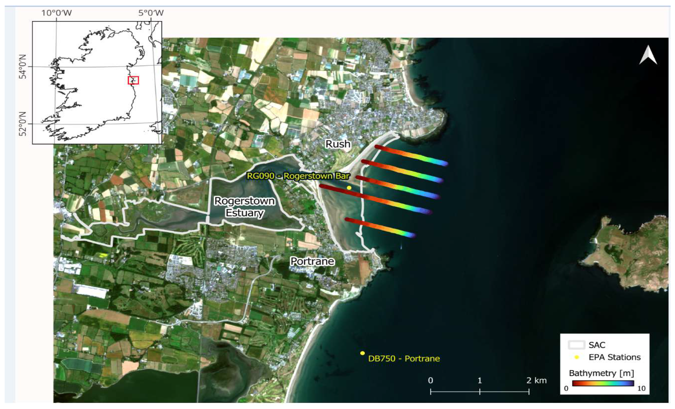
Figure 1. Study area (inset red box) located between the beaches of Portrane and South Rush in North County Dublin, Ireland. Multibeam data points collected by the GSI in 2021 are overlapped in the image. The yellow points represent the locations of the EPA stations where the water quality data were collected (Table 1).
Remotesensing 17 03834 g001
Figure 2. Estimated GLM models versus actual depth scatterplots for ten images. In each plot, the black line represents the identity line where the estimated and actual depths coincide. The red lines represent limits of error of ±0.5 m. Axes are measured in meters (m).
Remotesensing 17 03834 g002
Figure 3. Estimated versus actual water depth (m) for the multi-image analysis Single-image 6 (top), and for the median (middle) an mean (bottom) reducers using all 10 composite images. The black line represents the 1:1 identity line where the estimated and actual depths coincide, and the red lines represent the ±0.5 m error limits.
Remotesensing 17 03834 g003
Figure 4. GLM residuals (m) across the study area, calculated as estimated depth minus observed depth (negative values indicate model underestimation; positive values indicate model overestimation). Red dashed lines indicate ±0.5 m error limits. A LOESS smoother (dashed blue line, span = 1.2) is shown on each panel. Top: Image 6. Single-image case (Image ID 6). Middle: C10 Median. Median composite of 10 images. Bottom: C10 Mean. Mean composite of 10 images.
Remotesensing 17 03834 g004
Figure 5. Trends across the best GLM combinations at each subset size (C1 to C10). For each k (1 to 10 images), the combination with the minimum MAE was selected. RMSE and MAE (m) use the left axis; WRS uses the right (see Section 2.5; lower is better). C10 denotes the all-images composite.
Remotesensing 17 03834 g005
Figure 6. Distribution of Isolated outliers (red) and Persistent outliers (blue) in the results of the mean-reduced multi-image analysis using all 10 images. All other points that were not classified as outliers are coloured grey. The black line represents the identity line where the estimated and actual depths coincide, and the red lines represent the ±0.5 m error limits.
Remotesensing 17 03834 g006
Figure 7. Spatial distribution of depth residuals (model vs. validation) along the survey transects for the best-performing GLM multi-image combination (C4; four-image mean composite). Residuals are classified as −2.91 to −0.5 m (green), −0.5 to 0.5 m (grey), and 0.5 to 1.64 m (orange). Background imagery: Sentinel-2.
Remotesensing 17 03834 g007
Table 1. Water properties from the EPA at two stations during the analysed period of April–September 2021. N/A: data are not available.
Station NoSurvey DateWater Depth (m)Secchi Disk (m)Chlorophyll a (µg/L)Salinity (‰)Temperature (°C)pH
RG09026 May 20212.814.1132.7812.38.2
RG0907 July 20212.521.3431.3115.88.1
DB7502 July 20206.34N/A33.3614.38.1
DB75018 August 20207.13N/A33.2016.68.1
Table 2. Sentinel-2 images considered in this study after applying the selection criteria, together with the date and tide height at the time of the image acquisition.
Image IDSentinel-2 TileDateTide (LAT) (m)
1S2B_MSIL2A_20210405T1143495 April 20211.14
2S2B_MSIL2A_20210415T11434915 April 20213.57
3S2A_MSIL2A_20210417T11331117 April 20212.64
4S2B_MSIL2A_20210422T11330922 April 20211.78
5S2B_MSIL2A_20210604T1143494 June 20211.50
6S2A_MSIL2A_20210716T11332116 July 20211.63
7S2A_MSIL2A_20210719T11435119 July 20211.03
8S2B_MSIL2A_20210721T11331921 July 20212.53
9S2A_MSIL2A_20210828T11435128 August 20212.31
10S2A_MSIL2A_20210914T11332114 September 20211.56
Table 3. Summary of model results for Stumpf, Lyzenga, and GLM across 10 Sentinel-2 images, including R2, RMSE, MAE, and WRS.
Image IDSentinel-2 TileDateModelR2RMSE (m)MAE (m)MBE (m)WRS
1S2B_MSIL2A_202104055 April 2021Stumpf0.3472.3411.8840.2620.358
Lyzenga0.8311.1360.8990.2380.124
GLM0.8511.0960.8550.3320.115
2S2B_MSIL2A_2021041515 April 2021Stumpf0.7691.3041.0120.0790.154
Lyzenga0.8281.1240.884−0.0670.124
GLM0.8631.0170.761−0.0220.105
3S2A_MSIL2A_2021041717 April 2021Stumpf0.7451.4031.1180.0900.169
Lyzenga0.8331.1150.8690.0170.122
GLM0.8391.0900.8240.0100.117
4S2B_MSIL2A_2021042222 April 2021Stumpf0.8201.1660.8940.1810.129
Lyzenga0.8541.0360.7750.1010.109
GLM0.8641.0050.7350.1170.103
5S2B_MSIL2A_202106044 June 2021Stumpf0.6101.7041.3640.2350.232
Lyzenga0.8790.9810.7870.1190.099
GLM0.9160.8240.6370.2380.077
6S2A_MSIL2A_2021071616 July 2021Stumpf0.4711.9871.5480.2750.294
Lyzenga0.8880.9190.7280.0300.092
GLM0.9200.7730.583−0.0720.072
7S2A_MSIL2A_2021071919 July 2021Stumpf0.6561.6931.3860.4720.217
Lyzenga0.8840.9270.7160.1040.095
GLM0.9020.8670.6650.1590.085
8S2B_MSIL2A_2021072121 July 2021Stumpf0.7491.4241.1300.0470.169
Lyzenga0.8850.9690.7800.1240.097
GLM0.9040.8810.6790.0770.084
9S2A_MSIL2A_2021082828 August 2021Stumpf0.5861.7771.467−0.0650.246
Lyzenga0.7921.2401.0030.00950.144
GLM0.8191.1560.892−0.06060.129
10S2A_MSIL2A_2021091414 September 2021Stumpf0.7091.4751.1950.16240.186
Lyzenga0.8221.1490.9660.06010.130
GLM0.9220.8020.6690.26610.075
Table 4. Comparison of the performance metrics achieved by applying the GLM to image ID 6 and the mean- and median-reduced full set of image combinations.
Image IDImagesSingle/
Multi-Image
ReducerR2RMSE (m)MAE (m)MBE (m)WRS
616 July 2021Single-0.920.770.58−0.070.072
C10All 10 images combinedMulti-imageMean0.970.500.39−0.130.040
Median 0.861.000.83−0.050.108
Table 5. Results for the ten best multi-image combinations using the mean reducer based on all 1023 possible combinations.
RankingCombination NumberNumber of ImagesImage IDsR2RMSE (m)MAE (m)WRS
129742, 5, 6, 80.9740.4460.3420.035
215735, 6, 80.9710.4630.3530.037
357152, 5, 6, 8, 100.9740.4500.3560.035
480362, 4, 5, 6, 8, 100.9740.4680.3560.036
581462, 5, 6, 7, 8, 90.9700.4690.3560.037
610552, 5, 6, 8, 90.9710.4740.3570.037
754862, 4, 5, 6, 7, 80.9720.4780.3580.037
856752, 5, 6, 7, 80.9710.4710.3590.037
994862, 3, 5, 6, 8, 100.9710.4770.3590.037
1081562, 5, 6, 7, 8, 100.9720.4720.3610.037
Table 6. Number of Isolated and Persistent outliers and % of the total number of validation points for the image. A total of 91 isolated outliers were identified across all images.
Image IDImage DateTotal OutliersIsolated OutliersPersistent OutliersValidation Points% Isolated Outliers% Persistent Outliers
15 April 202129111810851.0%1.7%
215 April 20212261610850.6%1.5%
317 April 202155262910852.4%2.7%
422 April 202146182810851.7%2.6%
54 June 202127101710850.9%1.6%
616 July 202129111810851.0%1.7%
719 July 20211851310850.5%1.2%
821 July 20211741310850.4%1.2%
928 August 20211301310850.0%1.2%
1014 September 202110110850.0%0.1%
Disclaimer/Publisher’s Note: The statements, opinions and data contained in all publications are solely those of the individual author(s) and contributor(s) and not of MDPI and/or the editor(s). MDPI and/or the editor(s) disclaim responsibility for any injury to people or property resulting from any ideas, methods, instructions or products referred to in the content.