Low-Cost Real-Time Remote Sensing and Geolocation of Moving Targets via Monocular Bearing-Only Micro UAVs

Highlights

What are the main findings?

• A bearing-only localization framework is proposed for micro UAVs operating over uneven terrain, combining a pseudo-linear Kalman filter (PLKF) with a sliding-window nonlinear least squares optimization to achieve real-time 3D positioning and motion prediction.
• An observability-enhanced flight trajectory planning method is designed based on the Fisher Information Matrix (FIM), which improves localization accuracy in flight experiments, with an average gain of up to 4.34 m.

What are the implications of the main findings?

• The method addresses the limitations of monocular cameras with scale ambiguity and lack of depth measurement, providing a practical solution for low-cost UAVs in remote sensing and moving target localization.
• The results suggest potential applications in emergency response, target monitoring, and traffic security, demonstrating the feasibility of high-accuracy localization on resource-constrained UAV platforms.

Abstract

Low-cost and real-time remote sensing of moving targets is increasingly required in civilian applications. Micro unmanned aerial vehicles (UAVs) provide a promising platform for such missions because of their small size and flexible deployment, but they are constrained by payload capacity and energy budget. Consequently, they typically carry lightweight monocular cameras only. These cameras cannot directly measure distance and suffer from scale ambiguity, which makes accurate geolocation difficult. This paper tackles geolocation and short-term trajectory prediction of moving targets over uneven terrain using bearing-only measurements from a monocular camera. We present a two-stage estimation framework in which a pseudo-linear Kalman filter (PLKF) provides real-time state estimates, while a sliding-window nonlinear least-squares (NLS) back end refines them. Future target positions are obtained by extrapolating the estimated trajectory. To improve localization accuracy, we analyze the relationship between the UAV path and the Cramér–Rao lower bound (CRLB) using the Fisher Information Matrix (FIM) and derive an observability-enhanced trajectory planning method. Real-flight experiments validate the framework, showing that accurate geolocation can be achieved in real time using only low-cost monocular bearing measurements.

1. Introduction

1.1. Background and Significance

Target localization is a key problem in aerial remote sensing, supporting applications such as high-resolution geographic mapping [1], target surveillance and tracking [2,3], land-resource monitoring [4], moving-target enclosure [5], and search-and-rescue missions [6]. With the miniaturization and cost reduction of unmanned aerial vehicles (UAVs), micro UAVs equipped with lightweight visual sensors have become valuable platforms for real-time data acquisition in both civilian and defense contexts. In these scenarios, geolocation depends on estimating the relative state between the UAV and ground targets from onboard observations, often under strict payload and energy constraints, complex terrain, and dynamic environments.

Although many tracking and localization techniques have been developed in remote sensing [7,8], aerospace [9,10], and robotics [11,12], bearing-only localization from monocular imagery remains particularly challenging due to scale ambiguity, lack of direct range measurements, and strong dependence on relative motion. To address these challenges, this paper (i) employs bearing-only measurements from a monocular gimbal camera for moving-target localization, (ii) quantifies how relative motion and UAV trajectories affect observability and estimation accuracy, and (iii) develops an observability-enhanced trajectory planning strategy for real-time geolocation performance.

1.2. Related Works

Previous studies have aimed to improve UAV-based visual detection and geographic localization capabilities [13,14,15,16,17,18]. Li et al. [13] proposed a detection algorithm based on the Swin Transformer network to improve image quality and target detection accuracy. Meng et al. [14] enhanced remote sensing photogrammetry accuracy through anomaly detection. Yang et al. [15] discussed UAV localization and control under occluded camera scenarios in remote sensing contexts. Savkin et al. [16] proposed a distributed navigation algorithm to monitor targets moving along curved roads. Guo et al. [17] developed a novel adaptive extended Kalman filter method for UAVs equipped with electro-optical pods to enhance localization accuracy. Zhou et al. [18] applied related methods to large fixed-wing UAVs operating at high altitudes.

However, micro UAVs are constrained by payload and power supply, limiting their capability to carry high-precision sensors such as electro-optical pods, thus typically equipped only with monocular gimbal cameras. Due to the inherent scale uncertainty and lack of direct distance measurement, accurately estimating the 3D pose of targets remains challenging. Current research on monocular camera-based localization mainly employs prior-based [19,20] and learning-based approaches [21,22]. Zhou et al. [19] used a flat terrain assumption and UAV altimeter measurements to approximate relative target heights, which is unsuitable for non-flat terrains. Pizani et al. [20] utilized Digital Elevation Models (DEMs) to provide height priors, but this requires large-scale maps unsuitable for micro UAVs. Wang et al. [21] and Yang et al. [22] recovered depth from monocular images through learning methods, but these involve complex training and high computational demands. Zhang et al. [23] proposed an approach without prior information, applicable only to stationary ground targets, with the difficulty of estimation increasing significantly at greater distances.

To address these challenges, we propose a bearing-only localization method that avoids direct depth measurements or scale priors, relying solely on angular measurements collected during continuous relative motion. This concept has proven viable in radar and maritime applications. Farina et al. [24] initially used radar bearings to estimate target 3D positions. Li et al. [25] applied angular measurements to localize maritime vessels. In aerospace and remote sensing, bearing-only methods have been widely utilized [26,27,28]. Chu et al. [26] applied the technique in spacecraft rendezvous and docking, while Wang et al. [27] and Li et al. [28] used it for UAV localization and aerial target navigation.

Because bearing-only measurements provide direction but not range, accurate estimation requires relative motion and multiple views. This creates two main challenges for UAV remote sensing. First, solving the problem hinges on estimating the target’s state between consecutive frames when both the UAV and the target are moving. In practice, incremental Kalman filtering like EKF and the PLKF [29,30,31] is commonly used, but fast maneuvers can accumulate inter-frame errors, and the nonlinear measurement model increases computational load, making high-precision real-time estimation difficult. Second, not all relative motions lead to the same 3D accuracy under noise; this is an issue of observability. Typical analyses use bearing rigidity, rank conditions, or information-theoretic tools. For example, Ferdowsi [29] studied 2D observability via matrix conditions, while Jiang [32] and Woffinden [33] analyzed the 3D single-target case under Gaussian noise using FIM/CRLB, showing that different motion patterns yield different minimum error bounds.

Beyond these foundations, several recent works focus explicitly on bearing-only localization and observability enhancement. Wang et al. [27] derive a 3D bearing-only helical homing law and reveal weak observability under proportional navigation guidance (PNG), motivating guidance that explicitly increases observability. Zheng et al. [34] propose a cooperative STT-R estimator that exploits bearing rates in a distributed RLS framework to improve observability and reduce velocity lag. In multi-robot settings, Lu et al. [35] present a concurrent-learning-based relative localization method that relaxes persistent excitation and enhances inter-robot observability during shape formation. For air-to-air scenarios, Liu et al. [36] combine detection, KF-based tracking, and interval replanning to maintain fixed-distance pursuit for 3D reconstruction of a non-cooperative UAV.

Compared with these studies, our work considers a single micro-UAV with bearing-only sensing over non-flat terrain and couples a PLKF→SW-NLS estimator with an FIM-driven, observability-enhancing trajectory planner. The entire pipeline runs onboard and is validated in real flight.

1.3. Contributions

To solve the challenge of localizing targets on non-flat terrains using bearing-only measurements from micro UAVs, this study proposes a comprehensive localization and trajectory planning framework addressing cumulative inter-frame errors and observability-enhanced trajectory design. The primary contributions are as follows.

(1) Bearing-Only 3D Localization Framework for Uneven Terrain: To address the limitations of prior studies that typically assume flat ground [19] or rely on DEM-based elevation priors [20], this paper develops a real-time localization framework that operates effectively over uneven terrain. It enables a micro-UAV equipped only with a monocular gimbal camera to perform 3D localization and prediction of moving targets. The framework has been validated through real flight experiments, demonstrating high-accuracy geolocation under low-cost conditions and providing a systematic solution for micro-UAV remote sensing.

(2) Two-Stage Fusion Algorithm with PLKF Front End and Sliding-Window Nonlinear Least-Squares Back End: We propose a two-stage structure that combines a PLKF based front end with a sliding-window optimization back end. The front end provides inter-frame priors and projects bearing residuals, while the back end corrects accumulated errors through a SW-NLS formulation. This design significantly improves estimation accuracy while maintaining real-time performance, making it suitable for onboard deployment on micro-UAVs. Compared with the traditional EKF method, the front end achieves a computation speed improvement of approximately 8 ms per frame and offers better numerical stability while maintaining comparable accuracy.

(3) FIM-Based Observability Analysis and Closed-Loop Trajectory Planning Method: By quantitatively analyzing observability under Gaussian noise using the Fisher Information Matrix (FIM), this work reveals how the relative motion between the UAV and the target influences localization accuracy. Based on this analysis, we develop an observability-enhancing trajectory planning method that yields a closed-form, easily implementable local-orbit design rule, executed in discrete form. Compared with [28], our method continuously improves observability during flight along the planned trajectory, forming a closed-loop information flow that integrates state estimation, observability analysis, trajectory optimization, and enhanced estimation. Real flight results show that the proposed trajectory improves localization accuracy by more than 4.34 m compared with direct pursuit and manual flight, demonstrating both the effectiveness and engineering practicality of the method.

1.4. Organization

The remainder of the paper is organized as follows. Section 2 describes the system overview and problem formulation. Section 3 details the PLKF-based motion estimation, sliding-window optimization, observability analysis, and trajectory planning. Section 4 presents real-flight experiments and comparative results. Section 5 concludes the paper.

2. Problem Formulation

2.1. System Overview

Considering that micro-UAVs equipped with inexpensive monocular cameras cannot directly measure the depth of targets during remote sensing tasks over uneven terrain, this paper proposes a real-time remote sensing target localization framework using bearing-only measurements. The overall system structure is shown in Figure 1, and its workflow and functionality are described as follows:

Firstly, the UAV collects ground images in real-time using the onboard monocular camera. Targets are detected using the YOLOv8 algorithm, providing real-time target coordinates in the image frame. After successful detection, image coordinates are converted into a unit direction vector $R_C$ in the camera frame using intrinsic parameters. Using extrinsic camera parameters and the UAV’s real-time pose data, this vector is further transformed into the world coordinate frame, yielding the direction measurement $R_W$.

Next, the UAV continuously observes the target from different positions and perspectives, acquiring multiple angle measurements. These measurements are sequentially stored, forming an observation data sequence for target localization. To obtain initial estimates required for optimization, the system employs the Pseudo-Linear Kalman Filter (PLKF) method, which estimates the target’s state contains position and velocity in real-time using a motion model each time new measurement data arrives.

Subsequently, a backend optimization procedure refines localization accuracy based on these measurements and initial estimates. Historical measurements beyond a certain threshold have negligible effects and add computational burden; hence, the system utilizes a fixed-length sliding window. Only the relative positions within this sliding window undergo nonlinear least-squares optimization, with earlier data serving as known prior positions. This approach maintains continuity and enhances computational efficiency.

Then, Bernstein polynomials fit the initially obtained target coordinates, generating a smooth and continuous trajectory curve. Recognizing that actual target motion is constrained by velocity and acceleration limits, a sliding-window mechanism is employed to extrapolate short-term trajectory predictions, providing necessary information for subsequent UAV trajectory optimization.

Finally, based on Fisher Information Matrix (FIM), the paper quantitatively analyzes how different UAV-target relative trajectories affect localization precision under Gaussian noise. Leveraging insights from this observability analysis, an observability-enhanced UAV trajectory planning method is proposed. This method significantly improves localization accuracy, is easy to implement, and does not require strictly tracking precise predefined paths. The integration of bearing-only localization and observability-enhanced trajectory planning effectively enhances the efficiency and accuracy of remote sensing tasks over uneven terrain. The overall workflow is shown in Figure 1.

2.2. Measurement Model

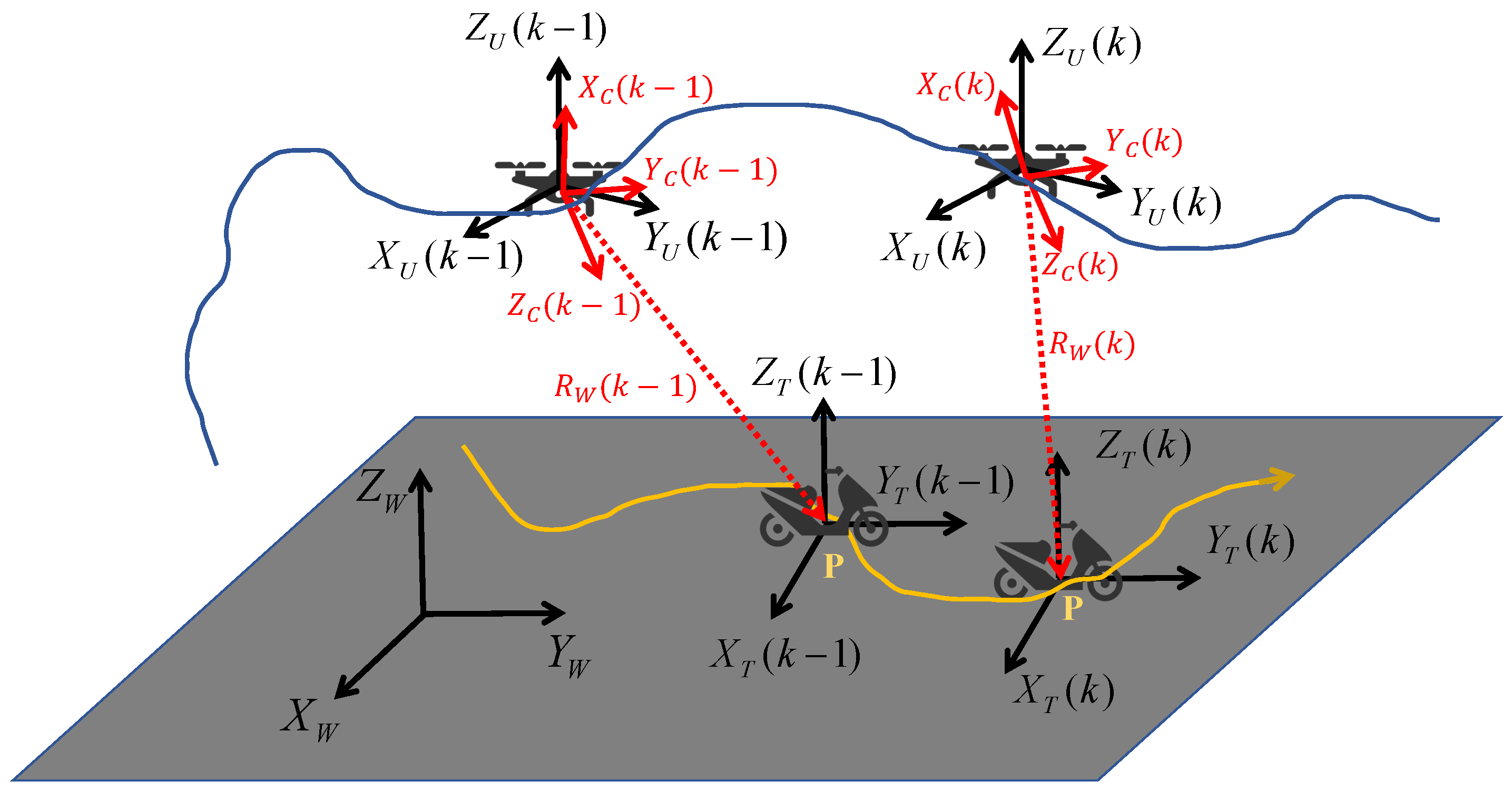
To clearly formulate the mathematical modeling of remote sensing target localization, we define four coordinate systems: the world coordinate system W, the UAV body coordinate system U, the target body coordinate system T, and the camera coordinate system C onboard the UAV. The world coordinate system W is fixed to the ground and serves as an inertial reference frame. The origin of the UAV body coordinate system U is located at the UAV’s center of mass, with its x-axis pointing towards the nose, y-axis pointing to the left wing, and z-axis pointing upwards, forming a right-handed coordinate system. Similarly, the target coordinate system T has its origin at the target’s center of mass, with axes defined identically to the UAV body coordinate system. The camera coordinate system C is centered at the camera’s optical center, with the z-axis along the optical axis, and the x- and y-axes forming a right-handed system on the imaging plane. Figure 2 shows the relationships among these coordinate frames.

The geographical localization of targets based on visual measurements can be achieved by combining the camera imaging model and rigid body transformations. Consider a ground target P, whose projection onto the camera imaging plane is denoted as $P_T$. The position of the target P in the world coordinate system can be represented as:

$$P_W=P_C+\lambda ·R_c^w·R_C,$$

(1)

where $P_C$ denotes the camera’s optical center position in the world coordinate system W, $R_c^w$ is the rotation matrix from the camera coordinate system C to the world coordinate system W, $R_C$ is the unit direction vector from the camera to the target in the camera coordinate system C, and $\lambda$ represents the scale factor, i.e., the actual distance from the camera optical center to the target point.

Using the pinhole camera model, the unit direction vector $R_C$ can be expressed in terms of pixel coordinates $(u,v)$ on the image plane and camera focal length f as:

$$R_C={\displaystyle \frac{1}{\sqrt{u^2+v^2+f^2}}}{(u,v,f)}^{\mathrm{T}}.$$

(2)

Substituting this into the target position equation, we obtain the target position in the world coordinate system:

$${(x_w,y_w,z_w)}^{\mathrm{T}}={(x_c,y_c,z_c)}^{\mathrm{T}}+\lambda ·R_c^w·{\displaystyle \frac{1}{\sqrt{u^2+v^2+f^2}}}{(u,v,f)}^{\mathrm{T}}.$$

(3)

Since monocular vision cannot directly measure the actual distance $\lambda$ from the camera to the target (due to scale ambiguity), we rearrange this expression to derive the explicit formula for the scale factor:

$$\lambda ={\displaystyle \frac{(z_w-z_c)\sqrt{u^2+v^2+f^2}}{{\mathbf{e}}_z{R}_c^w{(u,v,f)}^{\mathrm{T}}}}.$$

(4)

Here, ${\mathbf{e}}_z=(0,0,1)$ denotes the direction of the z-axis in the world coordinate system. Substituting the scale factor back into the position expression, we obtain the target’s horizontal position:

$${(x_w,y_w)}^{\mathrm{T}}={(x_c,y_c)}^{\mathrm{T}}+(z_w-z_c){\displaystyle \frac{\sqrt{u^2+v^2+f^2}}{{\mathbf{e}}_z{R}_c^w{(u,v,f)}^{\mathrm{T}}}}\left[\begin{array}{ccc}1& 0& 0\\ 0& 1& 0\end{array}\right]R_c^w{(u,v,f)}^{\mathrm{T}}.$$

(5)

The rotation matrix $R_c^w$ is determined by the following chain relation:

$$R_c^w=R_u^w{R}_c^u,$$

where $R_c^u$ represents the extrinsic rotation matrix between the camera and the UAV, a time-varying parameter due to gimbal movements, calculated in real-time from camera-gimbal calibration and measured gimbal rotation angles. $R_u^w$ is the UAV’s attitude rotation matrix in the world coordinate system, measured by the UAV’s attitude and position sensors. The camera focal length f is obtained through camera calibration, and $(u,v)$ are the detected target image coordinates. The camera optical center position is determined by the UAV’s onboard GPS device and camera extrinsic parameters.

Equation (5) provides a clear geometric method to derive the target’s three-dimensional coordinates from two-dimensional image data. However, as each image measurement provides only two independent equations, monocular visual localization inherently suffers from depth ambiguity. Therefore, additional constraints or prior information are required to determine the complete 3D coordinates. A common assumption in UAV localization tasks is the flat ground assumption, assuming negligible ground elevation changes. In practical scenarios, the relative altitude between UAV and target $h=z_U-z_T$ can initially be approximated using UAV GPS altitude information. This approximation provides a feasible initial guess for optimization. Once the initial estimate of the target position is established, subsequent optimizations iteratively refine the target location using the previously estimated position, a method proven feasible in [37].

For accurate 3D target position estimation, besides obtaining direction vectors $R_W$ at each measurement, the UAV state information (position and velocity) at discrete times $t_k$ must also be acquired:

$${\mathcal{S}}_U^{6D}=\left\{(P_U\left(k\right),V_U\left(k\right))\right|k=1,2,\dots ,n\},$$

(6)

with

$$P_U\left(k\right)\in {\mathbb{R}}^3,V_U\left(k\right)\in {\mathbb{R}}^3.$$

Thus, at each measurement time $t_k$, the system records direction vector $R_W\left(k\right)$, UAV position $P_U\left(k\right)$, and UAV velocity $V_U\left(k\right)$. These measurements form a discrete time-sequence:

$${\mathcal{S}}_U=\left\{(R_W\left(k\right),P_U\left(k\right),V_U\left(k\right))\right|k=1,2,\dots ,n\}.$$

(7)

Given that measurement data accumulate over time and early data’s influence diminishes, we adopt a dynamic sliding-window approach, maintaining a window of fixed length L:

$${\mathcal{S}}_U^L=\left\{(R_W\left(k\right),P_U\left(k\right),V_U\left(k\right))\right|k=t-L+1,\dots ,t\}.$$

(8)

Additionally, reasonable prior estimations of target motion between two measurements are necessary to achieve stable nonlinear least-squares optimization. The prior estimation of target states between observations is derived using individual measurement data and motion models, detailed further in Section 3. Figure 2 illustrates the process of bearing-only measurements of the target by the UAV during its motion.

3. Methodology

3.1. Inter-Frame Target Motion Estimation Based on Bearing-Only Measurements

The target motion between two consecutive frames from time $t(k-1)$ to $t\left(k\right)$ can be estimated using the angle measurements obtained at time $t\left(k\right)$. In this section, the relative target motion is modeled using orthogonal projection vectors and pseudo-linear Kalman filtering (PLKF). We systematically describe the mathematical modeling, filtering steps, and characteristics of the inter-frame motion estimation.

Consider the measurement at time $t\left(k\right)$. The UAV state, comprising position and velocity in the world coordinate system W, is denoted as:

$${\mathcal{S}}_U^{6D}\left(k\right)=(P_U\left(k\right),V_U\left(k\right)),$$

and the target state as:

$${\mathcal{S}}_T^{6D}\left(k\right)=(P_T\left(k\right),V_T\left(k\right)).$$

The relative state between the UAV and the target, which is to be estimated, is expressed as:

$$S\left(k\right)={\left[{(P_U\left(k\right)-P_T\left(k\right))}^{\top },{(V_U\left(k\right)-V_T\left(k\right))}^{\top }\right]}^{\top }\in {\mathbb{R}}^6.$$

(9)

The direction vector from the UAV to the target, measured by the monocular gimbal camera, is defined as:

$$R_W\left(k\right)={\displaystyle \frac{P_T\left(k\right)-P_U\left(k\right)}{\parallel P_T\left(k\right)-P_U\left(k\right)\parallel }}\in {\mathbb{R}}^3,\parallel R_W\left(k\right)\parallel =1.$$

(10)

Due to Gaussian measurement noise $\mu \sim \mathcal{N}(0,\mathsf{\Sigma })$, where $\mathsf{\Sigma }={\sigma }^2{I}_3$, the noisy measurement is expressed as:

$${\tilde{R}}_W\left(k\right)=R_W\left(k\right)+\mu .$$

(11)

Given the visual detection frequency of approximately 15–30 Hz, both UAV and target motions can be reasonably approximated as constant velocity within the small interval $\Delta t=t\left(k\right)-t(k-1)$. The kinematic state equations for the target and UAV are:

$$S_T^{6D}\left(k\right)=A{S}_T^{6D}(k-1)+Bw\left(k\right),$$

(12)

and

$$S_U^{6D}\left(k\right)=A{S}_U^{6D}(k-1)+Bv\left(k\right),$$

(13)

where

$$A=\left[\begin{array}{cc}{I}_3& \Delta t{I}_3\\ 0_3& I_3\end{array}\right],B=\left[\begin{array}{c}{\displaystyle \frac{1}{2}}\Delta t^2{I}_3\\ \Delta t{I}_3\end{array}\right],$$

(14)

with

$$w\left(k\right)\sim \mathcal{N}(0,{\mathsf{\Sigma }}_1),v\left(k\right)\sim \mathcal{N}(0,{\mathsf{\Sigma }}_2).$$

(15)

Considering UAV maneuvers, the combined relative motion model can be expressed as:

$$\widehat{S}\left(k\right)=A\left(\widehat{S}(k-1)+S_U^{6D}(k-1)\right)-S_U^{6D}\left(k\right).$$

(16)

Directly expressing the angle measurement ${\tilde{R}}_W\left(k\right)$ as a nonlinear function complicates subsequent computations. Hence, we introduce an orthogonal projection operator for pseudo-linearization. For any vector $\mathbf{v}\in {\mathbb{R}}^3$, the orthogonal projection operator $P_v$ is defined as:

$$P_v=I_3-{\displaystyle \frac{v{v}^{\top }}{{\parallel v\parallel }^2}},v\ne 0,$$

(17)

which projects vectors onto a plane perpendicular to v and satisfies $P_v^2=P_v=P_v^{\top }$. Multiplying both sides of ${\tilde{R}}_W\left(k\right)=R_W\left(k\right)+\mu$ by ${\lambda }_k{P}_{\tilde{R}\left(k\right)}$, where ${\lambda }_k=\parallel P_T\left(k\right)-P_U\left(k\right)\parallel$, yields:

$$0_3=P_{\tilde{R}\left(k\right)}\left(P_T\left(k\right)-P_U\left(k\right)\right)+\lambda \left(k\right)P_{\tilde{R}\left(k\right)}\mu .$$

(18)

Rewriting this equation using relative state $S\left(k\right)$, we obtain a pseudo-linear measurement equation:

$$0_3=H\left(k\right)S\left(k\right)+V_k\mu ,H\left(k\right)=\left[P_{\tilde{R}\left(k\right)},0_3\right],V_k=\lambda \left(k\right)P_{\tilde{R}\left(k\right)}.$$

(19)

Note that $H\left(k\right)$ and $V\left(k\right)$ are time-varying and $H\left(k\right)$ is rank-deficient. In practice, the predicted distance $\widehat{\lambda }\left(k\right)=\parallel \widehat{S}{\left(k\right)}_{1:3}^{-}\parallel$ substitutes the unknown $\lambda \left(k\right)$.

Based on this model and the measurement noise $\mu \left(k\right)\sim \mathcal{N}(0,{\mathsf{\Sigma }}_3)$, with ${\mathsf{\Sigma }}_3={\sigma }_3^2{I}_3$, the measurement covariance becomes:

$$T_k=V_k{\mathsf{\Sigma }}_3{V}_k^{\top }.$$

(20)

The PLKF algorithm consists of prediction and update steps. The prediction step is:

$$\widehat{S}{\left(k\right)}^{-}=A\left({\widehat{S}}_{k-1}+S_U^{6D}(k-1)\right)-S_U^{6D}\left(k\right),P{\left(k\right)}^{-}=AP(k-1)A^{\top }+BW\left(k\right)B^{\top }.$$

(21)

The Kalman gain is:

$$K\left(k\right)=P{\left(k\right)}^{-}H{\left(k\right)}^{\top }{\left(H\left(k\right)P{\left(k\right)}^{-}H{\left(k\right)}^{\top }+T\left(k\right)\right)}^{†},$$

(22)

where ${(·)}^{†}$ denotes the Moore-Penrose pseudo-inverse used due to rank deficiency of $H\left(k\right)$. As the measurement vector is zero, the state update equations are:

$$\widehat{S}\left(k\right)=\widehat{S}{\left(k\right)}^{-}-K\left(k\right)H\left(k\right)\widehat{S}{\left(k\right)}^{-},P\left(k\right)=(I_6-K\left(k\right)H\left(k\right))P{\left(k\right)}^{-}.$$

(23)

Through pseudo-linearization, measurement information is implicitly integrated into matrices $H\left(k\right)$ and $T\left(k\right)$, providing a linear formulation that facilitates prediction and updates. The PLKF method avoids nonlinear trigonometric expansions of angular measurements, enhancing numerical stability and computational efficiency, making it highly suitable for high-frequency visual measurements under constrained onboard computing resources.

3.2. Target Position Optimization Based on Nonlinear Least Squares

To mitigate the cumulative errors caused by the prolonged operation of pseudo-linear Kalman filtering (PLKF) and to fully exploit the geometric constraints from multi-frame bearing-only measurements, this paper designs a batch optimization sliding-window backend for discrete target position estimation on top of the PLKF frontend.

Let the sliding window length be L and the current frame index be k. The target positions to be estimated within the window are defined as:

$$\mathbf{S}={\left[P_T{(k-L+1)}^{\top },P_T{(k-L+2)}^{\top },\dots ,P_T{\left(k\right)}^{\top }\right]}^{\top }\in {\mathbb{R}}^{3\times L}.$$

For any frame $j\in [k-L+1,k]$ within the window, the whitened residual of direction measurements is defined as:

$${\tilde{r}}_j={\displaystyle \frac{1}{\sigma }}{P}_{\tilde{R}\left(j\right)}\left(P_T\left(j\right)-P_U\left(j\right)\right)\in {\mathbb{R}}^3,P_{\tilde{R}\left(j\right)}=I_3-{\tilde{R}}_W\left(j\right){\tilde{R}}_W^{\top }\left(j\right),$$

(24)

where $\sigma$ denotes the standard deviation of the bearing measurement. As $P_{\tilde{R}}{P}_{\tilde{R}}^{\top }=P_{\tilde{R}}$, the above residual is normalized to have a unit covariance matrix, constraining only two degrees of freedom orthogonal to the measurement direction. The unobserved depth dimension is supplemented by the PLKF prior.

PLKF provides an estimated relative position $\widehat{\mathbf{r}}\left(k\right)={\left(\widehat{S}\left(k\right)\right)}_{1:3}$ and associated covariance ${\mathbf{\Lambda }}_k=P_{k,r}$ for the latest frame k. The normalized prior residual is defined as:

$$r^{\mathrm{pri}}={\mathbf{L}}_k^{-{\displaystyle \frac{1}{2}}}\left(P_T\left(k\right)-\widehat{r}\left(k\right)\right),{\mathbf{L}}_k^{-{\displaystyle \frac{1}{2}}}{\mathbf{L}}_k^{-{\displaystyle \frac{1}{2}}\top }={\mathbf{\Lambda }}_k^{-1},$$

(25)

where ${\mathbf{L}}_k^{-{\displaystyle \frac{1}{2}}}$ is derived via Cholesky decomposition of the prior covariance matrix ${\mathbf{\Lambda }}_k$.

Combining these residual terms, the total optimization cost function for the sliding-window backend is defined as:

$$J\left(\mathbf{S}\right)=\sum _{j=k-L+1}^k|{\tilde{r}}_j{|}_2^2+{\left|r^{\mathrm{pri}}\right|}_2^2.$$

(26)

The first term minimizes the orthogonal plane error between the target positions and measurement rays, achieving geometric intersection across multiple frames. The second term provides stable depth anchoring from single-frame scale estimates provided by the PLKF frontend. Their weights are adaptively adjusted via their respective covariance matrices to prevent redundant information weighting.

Applying increments $\delta \mathbf{S}$ to the current estimate ${\mathbf{S}}^{\left(0\right)}$, the residuals can be linearized as:

$${\tilde{r}}_j\left(\mathbf{S}\right)\approx {\tilde{r}}_j+{\mathbf{J}}_j\delta \mathbf{S},{\mathbf{J}}_j=[\mathbf{0},\dots ,{\sigma }^{-1}{P}_{\tilde{R}\left(j\right)},\dots ,\mathbf{0}],$$

(27)

$$r^{\mathrm{pri}}\left(\mathbf{S}\right)\approx r^{\mathrm{pri}}+{\mathbf{J}}_{\mathrm{pri}}\delta \mathbf{S},{\mathbf{J}}_{\mathrm{pri}}=[\mathbf{0},\dots ,{\mathbf{L}}_k^{-{\displaystyle \frac{1}{2}}}].$$

(28)

The corresponding normal equation is:

$$\mathbf{H}\delta \mathbf{S}=-\mathbf{b},\mathbf{H}={\mathbf{J}}^{\top }\mathbf{J},\mathbf{b}={\mathbf{J}}^{\top }\mathbf{r},$$

(29)

where $\mathbf{J}$ stacks each frame’s ${\mathbf{J}}_j$ and prior ${\mathbf{J}}_{\mathrm{pri}}$, and $\mathbf{H}$ is a sparse block matrix that can be efficiently solved using sparse $LD{L}^{\top }$ decomposition.

When the window slides, $\mathbf{H}$ and $\mathbf{b}$ are partitioned by $[{\mathbf{T}}_{k-L+1},{\mathbf{S}}_{\mathrm{rem}}]$, marginalizing out the oldest state via Schur complement:

$$\tilde{\mathbf{H}}={\mathbf{H}}_{rr}-{\mathbf{H}}_{rm}{\mathbf{H}}_{mm}^{-1}{\mathbf{H}}_{mr},\tilde{\mathbf{b}}={\mathbf{b}}_r-{\mathbf{H}}_{rm}{\mathbf{H}}_{mm}^{-1}{\mathbf{b}}_m.$$

(30)

The resulting $(\tilde{\mathbf{H}},\tilde{\mathbf{b}})$ forms the new Gaussian prior for the next optimization loop, retaining full information and maintaining a 3D variable dimension.

Practically, the prior residuals generated when historical frames enter the window, as given by:

$$r_i^{\mathrm{pri}}={\mathbf{L}}_i^{-1/2}\left(P_T\left(i\right)-{\widehat{\mathbf{r}}}_i\right),i<k,$$

(31)

are continuously incorporated into the current Gaussian prior block through Schur complements as the window advances. This process ensures each window retains scale information from L frames and preserves the sparsity and conditioning of the least squares system.

The total cost function defined in (9) is solved using the Levenberg–Marquardt (LM) algorithm. LM linearizes $J\left(\mathbf{S}\right)$ at each iteration, solves the increment $\delta \mathbf{S}$ after damping $\mathbf{H}$ by adding $\lambda \mathbf{I}$, and iteratively updates $\mathbf{S}$ until convergence.

For this optimization, predicting the target’s future trajectory is necessary. Considering bounded continuity of velocity and acceleration, the trajectory is extrapolated using optimized past observations. Specifically, a time-decayed quadratic regularized least squares fitting is applied to the FIFO observation sequence ${\mathbf{Q}}_{\mathrm{target}}={\left\{({\mathbf{p}}_{t_i},t_i)\right\}}_{i=1}^L$, minimizing:

$$J_{\mathrm{pre}}=\sum _{i=1}^L{w}_{t_i}\parallel \widehat{B}\left(t_i\right)-{\mathbf{p}}_{t_i}{\parallel }_2^2+w_{p}L{\int }_{t_1}^{t_p}{\parallel {\widehat{B}}^{\left(2\right)}\left(t\right)\parallel }_2^{2}dt,w_{t_i}=tanh\left({\displaystyle \frac{k_t}{t_L-t_i}}\right),$$

(32)

The fitting cost $J_{\mathrm{pre}}$ consists of a time-decayed data term and a curvature regularization term. The first term minimizes the error between the fitted curve and the historical trajectory points, while the second term penalizes curvature to ensure the smoothness of the predicted trajectory and to avoid sharp fluctuations. $\widehat{B}\left(t\right)\in {\mathbb{R}}^3$ is an nth-order Bézier curve with control points $c_i$, $w_{t_i}$ downweights older samples, $w_p>0$ controls smoothness, and $t_p$ denotes the end of the prediction horizon. The velocity and acceleration bounds in Equation (33) are applied to $c_i$ through standard Bézier derivatives. subject to velocity and acceleration constraints:

$$\pm n(c^i-c^{i-1})\le \pm v_{mp},\pm n(n-1){\displaystyle \frac{(c^i-2c^{i-1}+c^{i-2})}{s_t}}\le \pm a_{mp}.$$

(33)

Solving this constrained quadratic programming (QP) yields an n-th order Bézier curve $\widehat{B}\left(t\right)$, producing a smooth, continuously differentiable trajectory over both observed and predicted intervals.

Equation (32) is updated in a sliding-window manner with each incoming visual detection. Since the visual detection frequency exceeds 15 Hz, the predicted target trajectory is rapidly updated as well, allowing the planner to keep up with the target’s frequent and irregular movements.

3.3. Observability-Enhanced Trajectory Planning

Building upon the PLKF-NLS-based bearing-only target localization framework, this section addresses another important issue: analyzing how the drone’s relative motion impacts the theoretical lower bound of target estimation accuracy under bearing measurements with Gaussian noise. Specifically, the analysis is carried out using the close relationship between the Fisher Information Matrix (FIM) and the Cramér–Rao lower bound (CRLB), where the CRLB defines the minimum achievable variance for any unbiased estimator. Even within our nonlinear optimization framework, the lowest achievable error bound is constrained by the CRLB. The FIM serves as a crucial tool for characterizing estimation precision, with its inverse providing a theoretical lower bound for the covariance of estimation errors. Based on this, we quantitatively analyze how different UAV motion patterns influence the lower bound of the target position estimation error and propose an observability-enhanced trajectory planning method for the UAV.

In this process, the camera measurement $R_C(u,v,f)$ is rotated into the world frame through $R_c^w=R_u^w{R}_c^u$, making it dependent on the UAV’s attitude but independent of its translation. The UAV position appears in the measurement model only through the relative displacement $P_T-P_U$ in the back-end residual and through the range $r_j$ used for weighting in the FIM (Equations (38)–(41)). Consequently, attitude errors act as angular noise on $R_W\left(k\right)$, as reflected in Equations (11) and (24).

The target positions to be estimated within the sliding window are denoted as:

$$\mathbf{S}={\left[P_T{(k-L+1)}^{\top },P_T{(k-L+2)}^{\top },\dots ,P_T{\left(k\right)}^{\top }\right]}^{\top }\in {\mathbb{R}}^{3\times L},$$

(34)

with the corresponding noisy bearing measurements:

$$\mathbf{R}=\left[{\tilde{R}}_W(k-L+1),{\tilde{R}}_W(k-L+2),\dots ,{\tilde{R}}_W\left(k\right)\right]\in {\mathbb{R}}^{3\times L},$$

(35)

where each noisy measurement ${\tilde{R}}_W\left(j\right)$ is the true bearing vector plus Gaussian noise:

$${\tilde{R}}_W\left(j\right)=R_W\left(j\right)+{\mu }_j,{\mu }_j\sim \mathcal{N}(0,{\sigma }^2{I}_3),j=k-L+1,\dots ,k.$$

(36)

According to the Cramér–Rao lower bound, the estimation error covariance matrix for any unbiased estimator $\widehat{\mathbf{S}}\left(\mathbf{R}\right)$ satisfies:

$$\mathbf{P}=\mathbb{E}\left[({\widehat{\mathbf{S}}}_3-{\mathbf{S}}_3){(\widehat{{\mathbf{S}}_3}-{\mathbf{S}}_3)}^{\top }\right]⪰{\mathbf{M}}^{-1},$$

(37)

where the FIM is defined as:

$$\mathbf{M}=-\mathbb{E}\left[{\displaystyle \frac{{\partial }^{2}log{p}_{\mathbf{R}|{\mathbf{S}}_3}}{\partial {\mathbf{S}}_3^2}}\right].$$

(38)

Under the assumptions of independent measurements with zero-mean Gaussian noise, the above FIM can be expressed as the sum of measurement information across frames within the sliding window:

$$\mathbf{M}=\sum _{j=k-L+1}^k{\left[{\displaystyle \frac{\partial R_W\left(j\right)}{\partial P_T\left(j\right)}}\right]}^{\top }{\mathsf{\Sigma }}_j^{-1}\left[{\displaystyle \frac{\partial R_W\left(j\right)}{\partial P_T\left(j\right)}}\right]=\sum _{j=k-L+1}^k{\displaystyle \frac{1}{{\sigma }_j^2{r}_j^2}}\left(I_3-R_W\left(j\right)R_W{\left(j\right)}^{\top }\right),$$

(39)

where the unit bearing vector is defined as $R_W\left(j\right)=(P_T\left(j\right)-P_U\left(j\right))/r_j$, and the range is $r_j=\parallel P_T\left(j\right)-P_U\left(j\right)\parallel$. Particularly, the matrix $(I-R_W{R}_W^{\top })$ is a projection operator that projects any vector onto the plane perpendicular to the bearing vector $R_W$. It is idempotent, satisfying ${(I-R_W{R}_W^{\top })}^2=I-R_W{R}_W^{\top }$, thus simplifying the form of the FIM.

In optimization, the determinant of the FIM, $det\mathbf{M}$, is inversely proportional to the volume of the probability ellipsoid for estimation error, and thus commonly used as an indicator of observational information content. However, directly optimizing $det\mathbf{M}$ becomes highly complex in three-dimensional space for a sliding window length $L>2$. Therefore, to obtain a more analytically convenient indicator, this section introduces the isotropy metric of the FIM:

$$J={∥\mathbf{M}-\overline{\lambda }{I}_3∥}_F^2,\overline{\lambda }=\frac{1}{3}tr\mathbf{M},$$

(40)

which measures the difference among the eigenvalues of the FIM. Specifically, $J=0$ indicates an ideal isotropic observational state. Expanding the above expression yields a more explicit formulation:

$$J={\parallel G\parallel }_F^2-{\displaystyle \frac{1}{3}}{S}_3^2,S=\sum _{j=k-L+1}^k{\displaystyle \frac{1}{{\sigma }_j^2{r}_j^2}},G=\sum _{j=k-L+1}^k{\displaystyle \frac{1}{{\sigma }_j^2{r}_j^2}}{R}_W\left(j\right)R_W{\left(j\right)}^{\top }.$$

(41)

From the above formulation, it is clear that two key factors influence the indicator J: the first involves the distance term $1/r_j^4$, and the second is related to the inner product between different measurement bearing vectors ${\left(R_W{\left(i\right)}^{\top }{R}_W\left(j\right)\right)}^2$. Evidently, shorter measurement distances and more orthogonal consecutive measurement bearings lead to a smaller J value and thus stronger observability.

Hence, we formulate the trajectory planning as a constrained optimization problem: minimizing the indicator J subject to safety distance $r_d$ and UAV dynamic constraints:

$$\underset{\left\{P_U\left(j\right)\right\}}{min}J\mathrm{s}.\mathrm{t}.\left\{\begin{array}{c}{r}_j\ge r_{min},\hfill \\ \parallel P_U(j+1)-P_U\left(j\right)\parallel \le v_{max}\Delta t,\hfill \\ \parallel V_U(j+1)-V_U\left(j\right)\parallel \le a_{max}\Delta t.\hfill \end{array}\right.$$

(42)

The FIM analysis indicates that maximizing the information content requires two conditions: (i) keeping the relative distance between UAV and target near the minimal allowed distance $r_d$; (ii) making the bearing vectors as orthogonal as possible within the sliding window, thereby minimizing their coupling terms ${\left(R_W{\left(i\right)}^{\top }{R}_W\left(j\right)\right)}^2$. Ideally, this corresponds to the UAV orbiting around the target at a constant angular velocity, forming a spherical trajectory with radius $r_d$. Due to UAV speed and vision sampling constraints, achieving perfectly orthogonal consecutive measurements is impractical; thus, ensuring spatially well-distributed measurements with significant angular differences is sufficient.

However, as the target is on the ground, the UAV can only orbit horizontally at fixed altitude z, implying a horizontal observation distance $r_h$. Through detailed analysis, we derive the optimal horizontal distance and angular velocity that maximize observability under speed limit $v_{max}$:

$$r_h^{★}=z,{\omega }^{★}={\displaystyle \frac{v_{max}}{z}},v^{★}=v_{max}.$$

(43)

Since the target also has a certain motion velocity, a margin should be reserved in practice.

Finally, explicitly incorporating the target’s motion speed, the discrete trajectory at each control interval $\Delta t$ can be given by:

$$\begin{array}{cc}\hfill P_U\left(k\right)& =P_U(k-1)+\dot{\widehat{B}}\left(t_k\right)\Delta t\hfill \\ \hfill & +r_h\left[cos({\theta }_0+(k-1)\Delta \theta )\mathbf{N}\left(t_k\right)+sin({\theta }_0+(k-1)\Delta \theta )(\mathbf{T}\left(t_k\right)\times \mathbf{N}\left(t_k\right))\right]\hfill \\ \hfill & -r_h\left[cos({\theta }_0+(k-2)\Delta \theta )\mathbf{N}\left(t_{k-1}\right)+sin({\theta }_0+(k-2)\Delta \theta )(\mathbf{T}\left(t_{k-1}\right)\times \mathbf{N}\left(t_{k-1}\right))\right],\hfill \end{array}$$

(44)

where $\Delta \theta =\omega \Delta t$ and the angular velocity constraint must satisfy:

$$|\dot{\widehat{B}}\left(t_k\right)|+\omega r_h\le v_{max},{\omega }^2{r}_h\le a_{max}.$$

(45)

At each perception update, we refit $\widehat{B}\left(t\right)$ over the latest window according to Equation (32) and recompute $T\left(k\right)$ and $N\left(k\right)$. Then, under the constraints of Equation (44), Equation (43) is executed once as a discrete update, followed by re-planning in the next cycle. This receding-horizon execution preserves the FIM-guided geometric properties (Equations (41) and (42)) while maintaining a fast and adaptive response to unknown and rapidly changing target motion.

This discrete expression explicitly reflects the combined effect of target motion and UAV orbiting motion, ensuring optimal observability while strictly adhering to dynamic constraints.

In contrast, position errors mainly alter the geometric structure that governs observability—specifically, the distances and the angles between adjacent bearing rays. As long as the trajectory shape remains approximately circular while dynamically orbiting the target, the variation of $R_W\left(k\right)$ relative to the planned trajectory will remain small.

4. Results

In this section, experiments were conducted in real-world environments to validate the effectiveness of the proposed method. Specifically, Section 4.1 describes our experimental site, the UAV platform used, and the experimental details. Section 4.2 analyzes the experimental results. Section 4.3 first investigates the performance of the NLS-based back-end optimization and compares the performance of the PLKF estimator with that of the EKF. Finally, it comprehensively analyzes the influence of trajectories on localization performance.

4.1. Flight Experiment Details

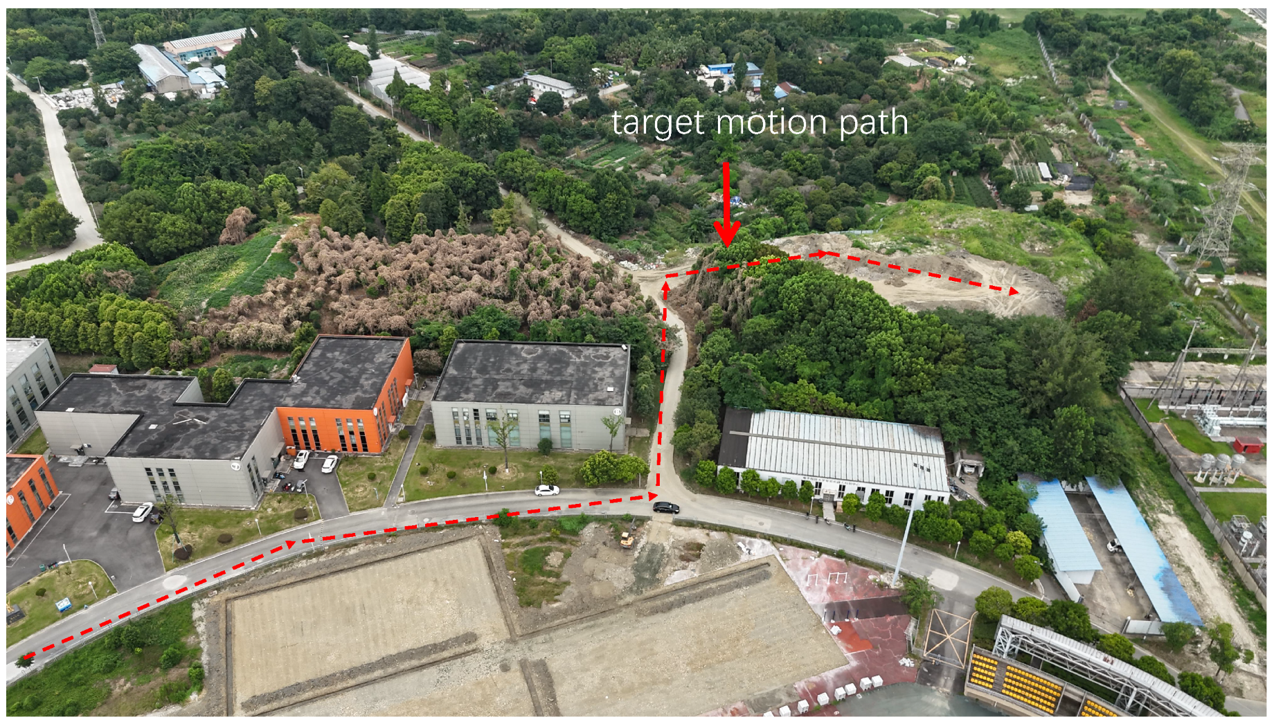
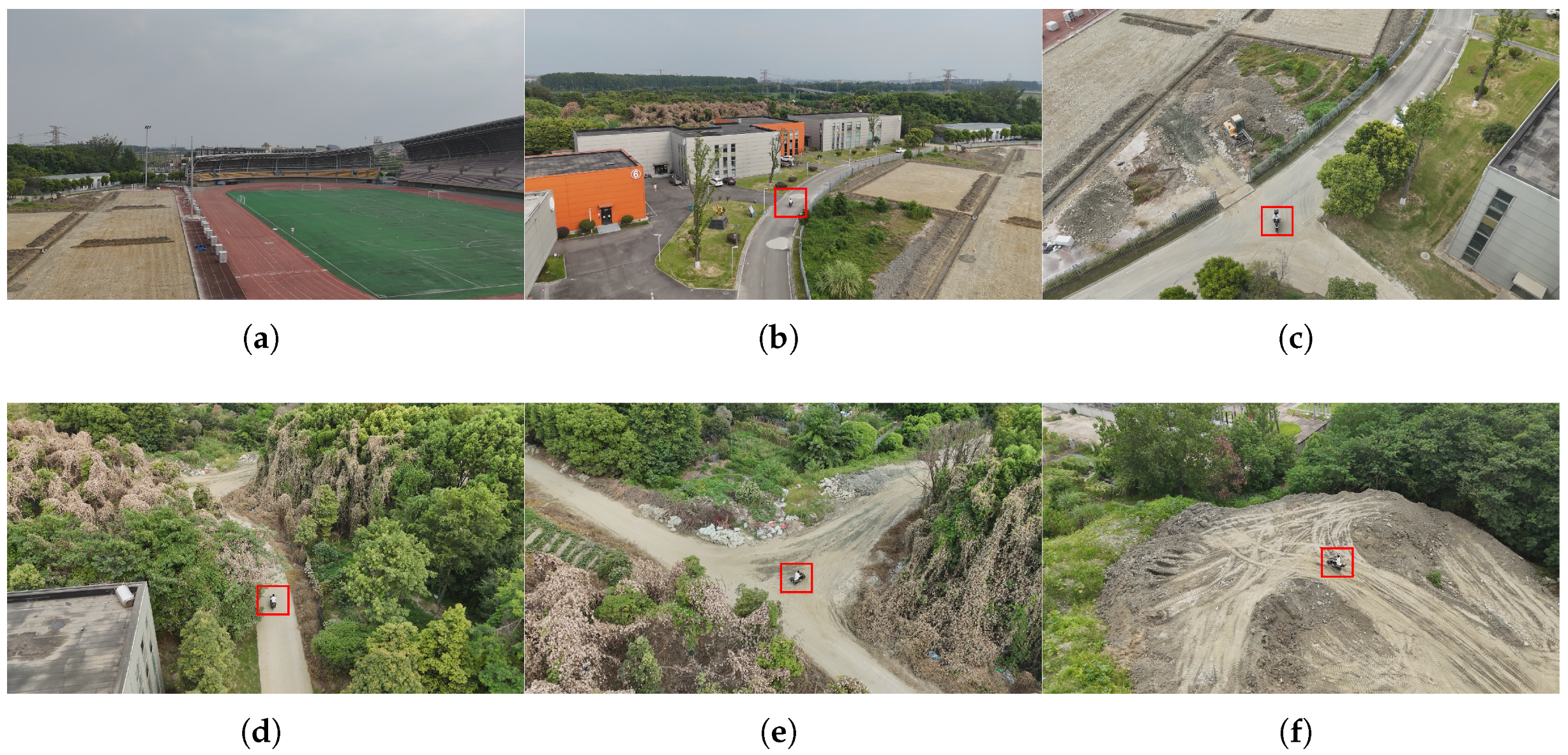
To validate the effectiveness of the proposed method, we used a typical remote-sensing scenario involving target localization using a micro UAV. Specifically, a motorbike moving in uneven terrain was selected as the target for tracking and localization. This scenario is prevalent in civilian applications, effectively demonstrating the general applicability of the proposed method in practical remote sensing tasks. The experimental site was a 200 m × 200 m area with varied terrain, where the elevation difference between the highest and lowest points reached 15 m. The airspace was open and provided reliable GNSS signal reception for the UAV at all locations. Additionally, the experiment was conducted under clear weather conditions, with wind speeds ranging between 1 m/s and 3 m/s, thus posing no significant impact on UAV flight stability. The target vehicle was driven randomly on uneven roads within the site and was equipped with a GNSS receiver to provide accurate ground-truth trajectory data for algorithm performance comparison. The experimental site is illustrated in Figure 3.

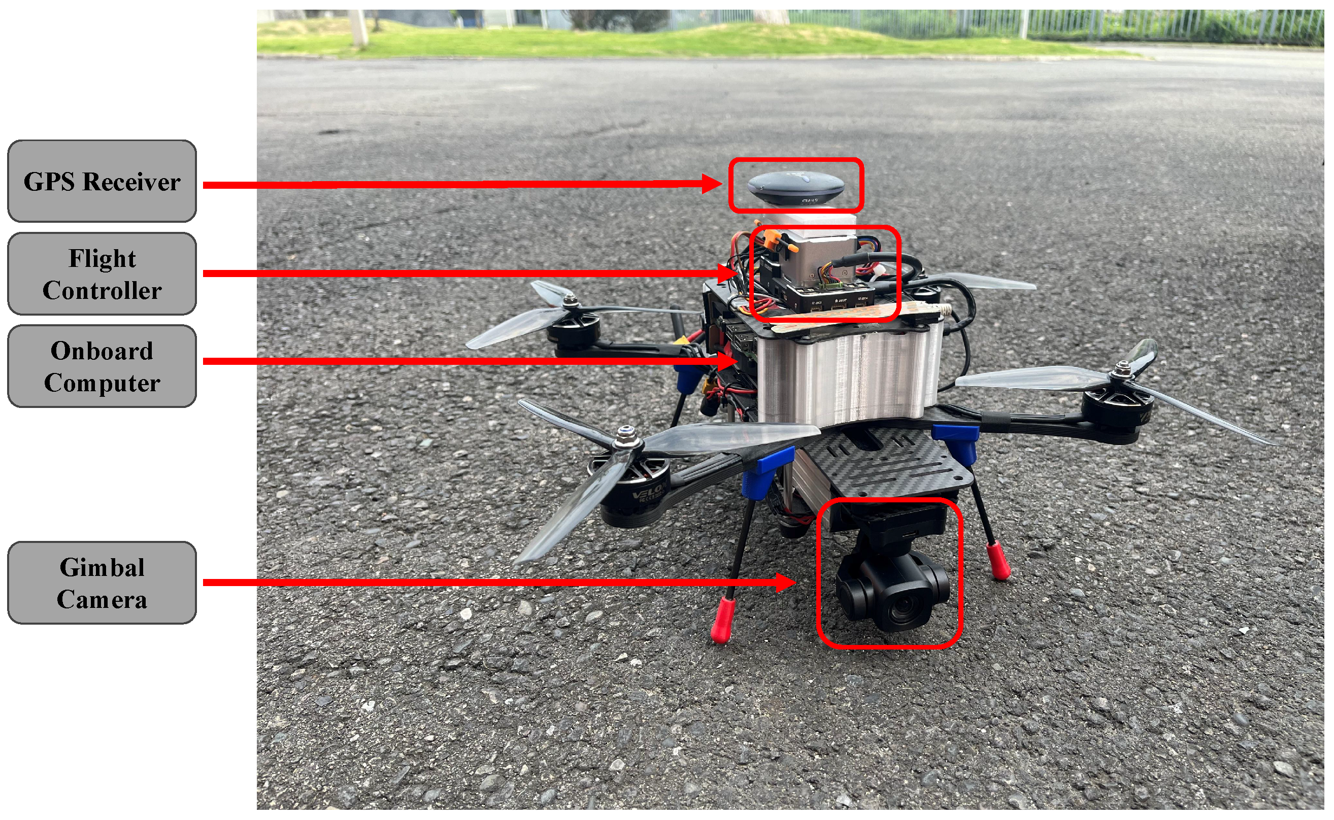
The experiment utilized a custom-designed micro UAV platform as shown in Figure 4. The UAV has a wheelbase of 35 cm, weighs only 1.3 kg, and has a maximum flight speed of 15 m/s, making it suitable for single-person portability and deployment. It is equipped with an onboard computing unit, an autonomous navigation system, and a vision system. Specifically, the onboard computing unit is an Intel NUC12 i7-1260P, the flight controller is a CUAV x7, and the GNSS receiver is a CUAV NEO3 pro. Navigation data is jointly obtained from the inertial measurement unit (IMU) of the flight controller and the GNSS receiver. The propulsion system comprises high-performance brushless motors and a 22.2 V, 2600 mAh lithium-polymer battery. The vision system includes a camera mounted on a three-axis gimbal and onboard target detection and tracking algorithms. The target detection algorithm, developed based on YOLOv8, identifies and locates the target vehicle in real-time within the camera’s field of view. The automatic gimbal tracking algorithm dynamically adjusts the gimbal orientation based on the target’s position in the image, ensuring the target remains centered and continuously records the gimbal’s three-axis angles. The camera has a resolution of 1920 × 1080 pixels and a frame rate of 25 Hz. These subsystems collectively enable the real-time fusion of geospatial localization, UAV status, and visual data. The software architecture of the entire system is based on ROS Noetic, and the nonlinear least-squares optimization problem is solved using the Ceres library. The trajectory planning generated waypoints are tracked using the model predictive control (MPC) method from [38], with control commands sent to the flight controller as angular velocities and throttle percentages.

In practical environments, wind enters Equations (12)–(15) as a bounded process disturbance. Its primary effect is geometric, causing slight deviations in the range $r_j$ and the bearing angles that determine the FIM. A cascaded PID controller running at 100 Hz is employed to counteract such position errors, and each motor provides a maximum thrust exceeding 3 kg, offering substantial control redundancy for wind resistance.

During the experiment, lasting over 200 s, the target vehicle continuously moved along the road while the UAV maintained a safe flight altitude of 25 m, ensuring both safe distance and continuous effective observation of the target.

4.2. UAV Target Localization Performance Analysis

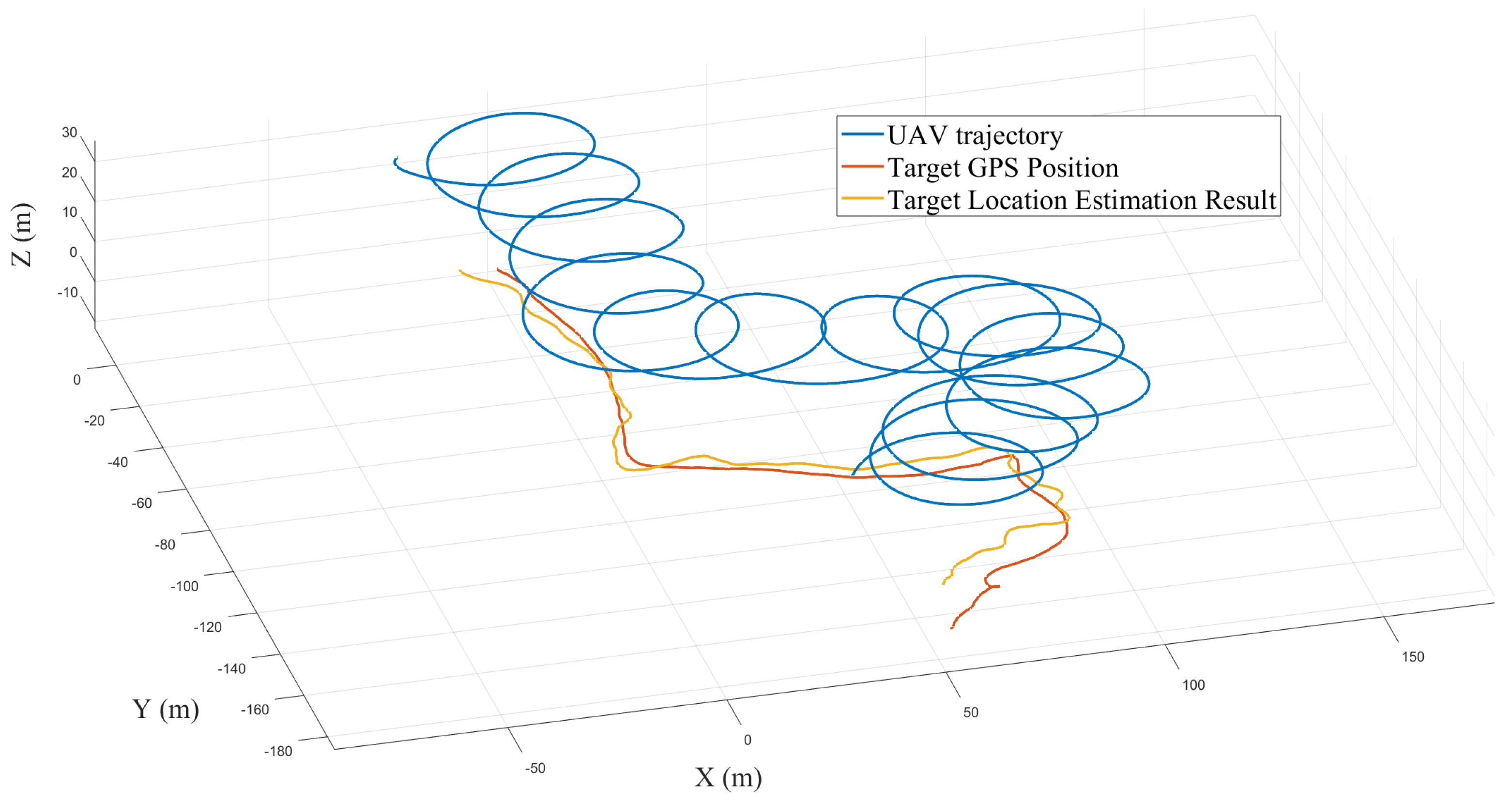
Figure 5 and Figure 6 together provide a comprehensive overview of the UAV-based target-tracking and localization experiment. Figure 5 presents the entire mission trajectories. the blue curve is the UAV flight path, the orange curve is the ground-truth target trajectory obtained from GNSS, and the yellow curve is the target trajectory estimated from bearing-only observations. Figure 6b–f illustrate the key stages from takeoff and target search to stable tracking and localization. We set the instant when the UAV completes takeoff and begins searching for the target (Figure 6) as time zero. At $t\approx 15$ s, the UAV reaches the vicinity of the target and switches to an observability-enhancing trajectory for stable tracking and localization, as shown in Figure 6b. During the experiment the target turns left at $t\approx 70$ s (Figure 6c), turns right at $t\approx 120$ s (Figure 6e), then climbs the slope and stops at the summit at $t\approx 220$ s, as shown in Figure 6f.

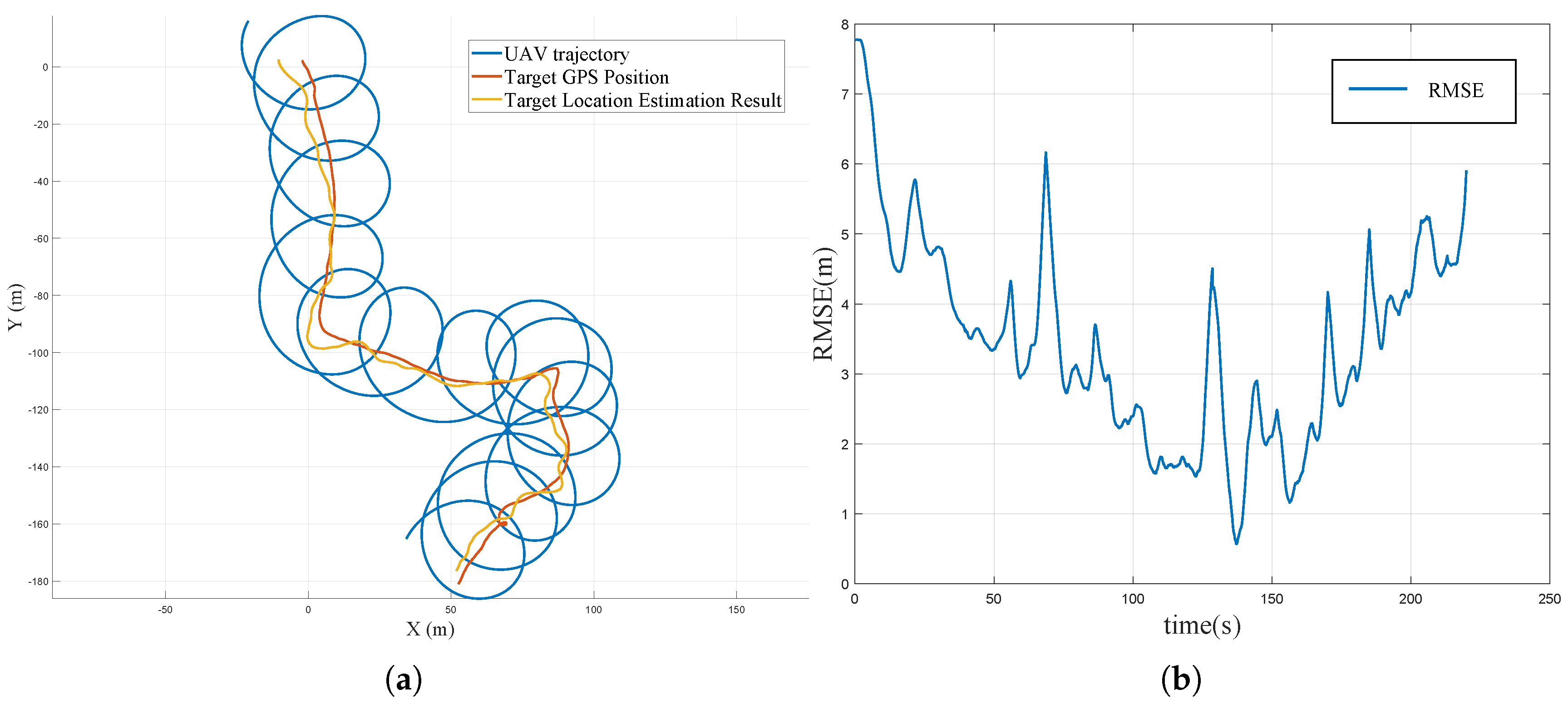
After take-off, the UAV first pans its gimbal camera to search for the target; once the target appears in the field of view, the camera continuously tracks it. In the initial localization frames, the UAV assumes a flat ground prior and flies almost straight toward the target to quickly reduce the range and iteratively refine the target position. At this stage, no observability-enhancing trajectory is used, so the localization accuracy is relatively low. As the UAV approaches, the horizontal distance r decreases, the bearing angle rate increases, and the uncertainty in the target position estimate decreases rapidly (Figure 7a). When $t\approx 15$ s and r reach the desired value of $r=25$ m, the UAV flies around the target at maximum linear speed until the end of the experiment ($t\approx 220$ s), producing high-precision estimates of the current and past positions of the target.

Figure 7b shows the RMSE between the estimated and true target positions throughout the experiment. The RMSE starts at 7.85 m, drops to 5.53 m as the UAV closes in, and further converges to 3.25 m once the observability-enhancing trajectory begins. A sharp left turn at $t\approx 70$ s briefly raises the RMSE to 6.13 m, but it quickly recovers to 2.93 m. A similar spike to 4.51 m occurs at the right turn at $t\approx 120$ s, then decreases to 3.88 m. The uphill motion slightly increases the RMSE to 4.03 m. During the whole process, the RMSE is 3.79m. Throughout the trial, the gimbal rapidly responds to target speed changes and the trajectory-prediction module adjusts the flight path in real time, allowing the estimation error to reconverge quickly. These results demonstrate that the proposed method maintains robust localization and tracking performance even when the target undergoes significant dynamic maneuvers.

4.3. Comparative Experiments

In this section, we first examine how back-end optimization influences overall system performance. We then disable the back-end and compare the performance gains achieved by the EKF [39] and PLKF front-end filtering algorithms. Finally, we analyze the impact of various flight-path geometries on localization accuracy, thereby providing a comprehensive validation of the effectiveness and advantages of the proposed method.

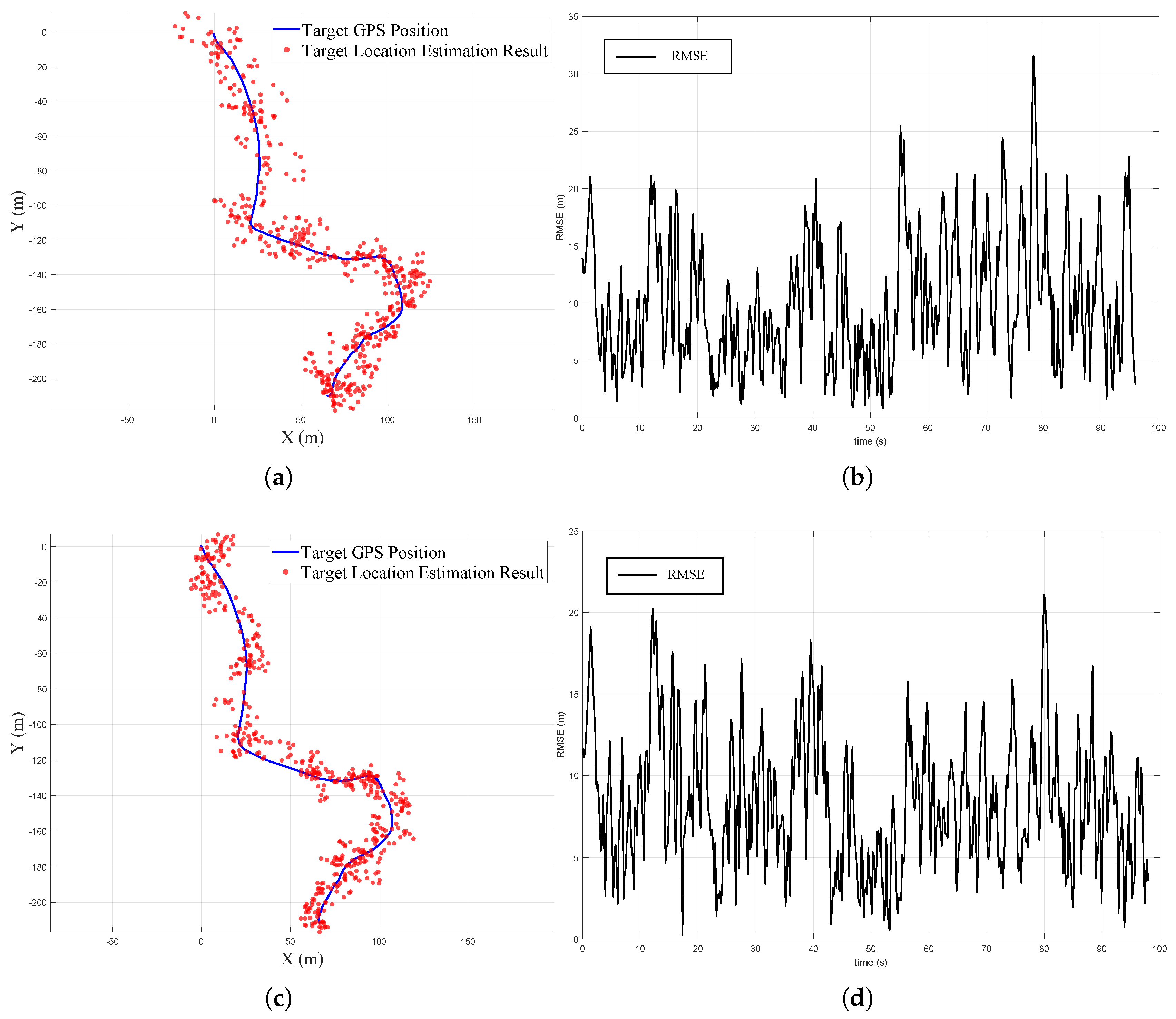
The specific experimental setup is as follows. A real flight dataset based on the observability-enhanced trajectory proposed in Section 3.3 was selected. During the flight, the UAV employed the proposed PLKF front end and Sliding-Window Nonlinear Least-Squares (SW-NLS) back end to perform real-time target localization and trajectory optimization. After the flight, the recorded data were replayed offline: first, the onboard real-time PLKF estimation results were extracted to produce the outcomes shown in Figure 8c,d; then, the same GNSS/IMU data, gimbal attitude angles, and image detection results were input into an independently implemented EKF estimator to compute and record its runtime and localization error, resulting in Figure 8a,b. This setup ensures a fair comparison between the two algorithms under identical input and environmental conditions.

Figure 8 illustrates the position-estimation results obtained after removing the back-end module and relying solely on the EKF or PLKF front end. Specifically, Figure 8a,b show the localization trajectory and RMSE obtained with the EKF front end, whereas Figure 8c,d present the corresponding results obtained with the PLKF front end. Under these conditions, the RMSE increased dramatically to 10.10 m for the EKF front-end and to 8.56 m for the PLKF front-end. Although PLKF consistently outperformed EKF in both computational speed and accuracy, it still could not achieve high localization accuracy when used independently. These results highlight that our proposed method, which combines the fast and effective PLKF front-end with the high-accuracy NLS back-end, achieves an optimal balance between computational speed and localization accuracy. Besides, the PLKF front-end had an inter-frame solving time ranging from 6 ms to 9 ms, while the EKF front-end required 14 ms to 18 ms, clearly demonstrating the computational speed advantage of PLKF.

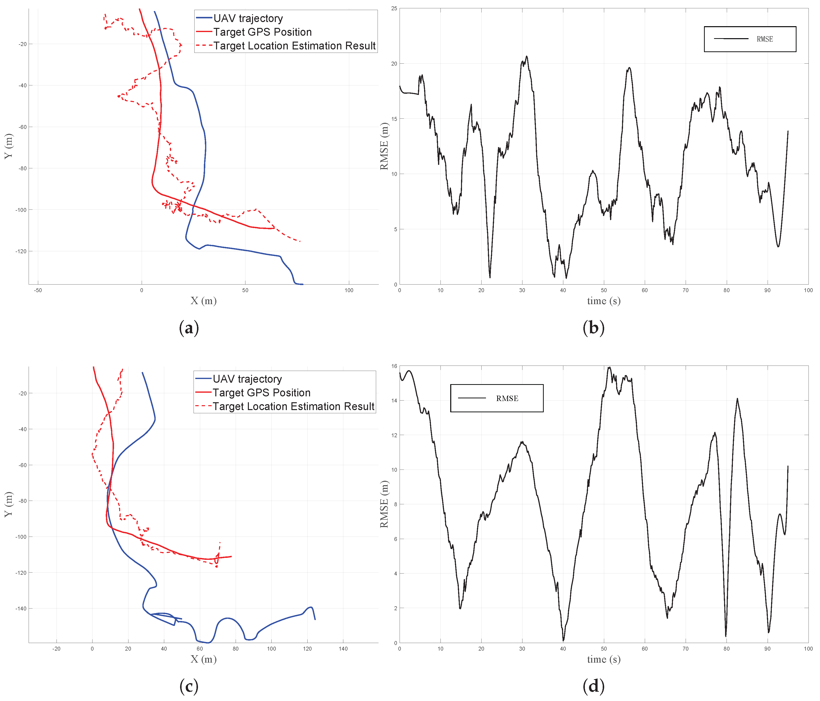
To evaluate the effectiveness of the proposed observability-enhanced trajectory, we further compared it with two commonly used UAV surveillance trajectories: the parallel-following trajectory and the manually operated trajectory. In the experiments, the ground target moved along the same route and within the same speed range as shown in Figure 5 and Figure 6, while the UAV maintained a flight altitude of approximately 25 m. Across all three experiments, the sensor configuration, detection algorithm, and localization method were kept identical.

First, we tested a commonly used parallel-following trajectory in remote sensing tasks; second, a professional operator manually piloted the UAV freely to track the target. In both sets of experiments, the UAV maintained a flight altitude of approximately 25 m. We recorded trajectory data and localization errors during these experiments and compared them against our observability-enhanced trajectory. Figure 9a–d show the four different flight trajectories and their localization errors relative to the actual target positions. The parallel-following trajectory resulted in an RMSE of 12.04 m, indicating a near-total localization failure. The RMSE for the manually operated trajectory was 8.13 m, respectively, significantly higher compared to our observability-enhanced trajectory, which achieved an RMSE of only 3.79 m. These results comprehensively demonstrate the effectiveness and superiority of the observability-enhanced trajectory proposed in this study in significantly improving remote sensing localization accuracy.

5. Conclusions

In this study, we systematically proposed and validated a UAV-based remote sensing target localization method using bearing-only measurements. The method comprises a localization framework integrating a front-end filtering algorithm with back-end optimization, along with an observability-enhanced trajectory planning strategy. Comparative experimental results demonstrated that combining the PLKF front-end with the sliding-window NLS back-end achieves an optimal balance between computational speed and localization accuracy. Specifically, the PLKF front-end significantly outperformed the EKF in computational efficiency, reducing inter-frame solving time by approximately two-thirds while maintaining comparable localization accuracy when paired with the NLS back-end.

Further experimental evaluations using various flight trajectories clearly highlighted the advantages of our proposed observability-enhanced trajectory. Compared to common tracking methods, such as parallel-following and manual operations, our approach substantially improved localization accuracy, significantly reducing RMSE. Specifically, the RMSE achieved with the observability-enhanced trajectory was only 3.79 m.

In conclusion, the localization method combining the fast PLKF front-end, high-precision NLS optimization, and observability-enhanced trajectory planning provides a robust and efficient solution for remote sensing target localization tasks, demonstrating strong potential for practical applications in various UAV-based sensing scenarios.

References

1. Cheng, Z.; Gong, W.; Jaboyedoff, M.; Chen, J.; Derron, M.-H.; Zhao, F. Landslide Identification in UAV Images Through Recognition of Landslide Boundaries and Ground Surface Cracks. Remote Sens. 2025, 17, 1900. [Google Scholar] [CrossRef]
2. de Moraes, R.S.; de Freitas, E.P. Multi-UAV Based Crowd Monitoring System. IEEE Trans. Aerosp. Electron. Syst. 2020, 56, 1332–1345. [Google Scholar] [CrossRef]
3. Li, W.; Yan, S.; Shi, L.; Yue, J.; Shi, M.; Lin, B.; Qin, K. Multiagent Consensus Tracking Control over Asynchronous Cooperation–Competition Networks. IEEE Trans. Cybern. 2025, 55, 4347–4360. [Google Scholar] [CrossRef] [PubMed]
4. Cao, Y.; Huang, X. A Coarse-to-Fine Weakly Supervised Learning Method for Green Plastic Cover Segmentation Using High-Resolution Remote Sensing Images. ISPRS J. Photogramm. Remote Sens. 2022, 188, 157–176. [Google Scholar] [CrossRef]
5. Li, W.; Yue, J.; Shi, M.; Lin, B.; Qin, K. Neural Network-Based Dynamic Target Enclosing Control for Uncertain Nonlinear Multi-Agent Systems over Signed Networks. Neural Netw. 2025, 184, 107057. [Google Scholar] [CrossRef] [PubMed]
6. Lyu, M.; Zhao, Y.; Huang, C.; Huang, H. Unmanned Aerial Vehicles for Search and Rescue: A Survey. Remote Sens. 2023, 15, 3266. [Google Scholar] [CrossRef]
7. Liu, C.; Peng, S.; Li, S.; Qiu, H.; Xia, Y.; Li, Z.; Zhao, L. A Novel EAGLe Framework for Robust UAV-View Geo-Localization. IEEE Trans. Geosci. Remote Sens. 2025, 63, 5629917. [Google Scholar] [CrossRef]
8. Zhou, S.; Fan, X.; Wang, Z.; Wang, W.; Zhang, Y. High-Order Temporal Context-Aware Aerial Tracking with Heterogeneous Visual Experts. Remote Sens. 2025, 17, 2237. [Google Scholar] [CrossRef]
9. Kim, J.; Lee, D.; Cho, K.; Kim, J.; Han, D. Two-Stage Trajectory Planning for Stable Image Acquisition of a Fixed Wing UAV. IEEE Trans. Aerosp. Electron. Syst. 2014, 50, 2405–2415. [Google Scholar] [CrossRef]
10. Sun, N.; Zhao, J.; Shi, Q.; Liu, C.; Liu, P. Moving Target Tracking by Unmanned Aerial Vehicle: A Survey and Taxonomy. IEEE Trans. Ind. Inform. 2024, 20, 7056–7068. [Google Scholar] [CrossRef]
11. Zhang, T.; Li, C.; Zhao, K.; Shen, H.; Pang, T. ROAR: A Robust Autonomous Aerial Tracking System for Challenging Scenarios. IEEE Robot. Autom. Lett. 2025, 10, 7571–7578. [Google Scholar] [CrossRef]
12. Tian, R.; Ji, R.; Bai, C.; Guo, J. A Vision-Based Ground Moving Target Tracking System for Quadrotor UAVs. In Proceedings of the 2023 IEEE International Conference on Unmanned Systems (ICUS), Hefei, China, 20–22 October 2023; pp. 1750–1754. [Google Scholar] [CrossRef]
13. Li, R.; Zhao, X. LSwinSR: UAV Imagery Super-Resolution Based on Linear Swin Transformer. IEEE Trans. Geosci. Remote Sens. 2024, 62, 5641013. [Google Scholar] [CrossRef]
14. Meng, C.; Yang, H.; Jiang, C.; Hu, Q.; Li, D. Improving UAV Remote Sensing Photogrammetry Accuracy Under Navigation Interference Using Anomaly Detection and Data Fusion. Remote Sens. 2025, 17, 2176. [Google Scholar] [CrossRef]
15. Yang, H.; Dong, H.; Zhao, X. Safety-Critical Control Allocation for Obstacle Avoidance of Quadrotor Aerial Photography. IEEE Control Syst. Lett. 2024, 8, 1973–1978. [Google Scholar] [CrossRef]
16. Savkin, A.V.; Huang, H. Navigation of a UAV Network for Optimal Surveillance of a Group of Ground Targets Moving Along a Road. IEEE Trans. Intell. Transp. Syst. 2022, 23, 9281–9285. [Google Scholar] [CrossRef]
17. Guo, Z.; Zhao, F.; Sun, Y.; Chen, X.; Wu, R. Research on Target Localization in Airborne Electro-Optical Stabilized Platforms Based on Adaptive Extended Kalman Filtering. Measurement 2024, 234, 114794. [Google Scholar] [CrossRef]
18. Zhou, X.; Jia, W.; He, R.; Sun, W. High-Precision Localization Tracking and Motion State Estimation of Ground-Based Moving Target Utilizing Unmanned Aerial Vehicle High-Altitude Reconnaissance. Remote Sens. 2025, 17, 735. [Google Scholar] [CrossRef]
19. Zhou, Y.; Tang, D.; Zhou, H.; Xiang, X. Moving Target Geolocation and Trajectory Prediction Using a Fixed-Wing UAV in Cluttered Environments. Remote Sens. 2025, 17, 969. [Google Scholar] [CrossRef]
20. Pizani Domiciano, M.A.; Shiguemori, E.H.; Vieira Dias, L.A.; de Cunha, A.M. Particle Collision Algorithm Applied to Automatic Estimation of Digital Elevation Model From Images Captured by UAV. IEEE Geosci. Remote Sens. Lett. 2018, 15, 1630–1634. [Google Scholar] [CrossRef]
21. Wang, Y.; Li, H.; Li, X.; Wang, Z.; Zhang, B. UAV Image Target Localization Method Based on Outlier Filter and Frame Buffer. Chin. J. Aeronaut. 2024, 37, 375–390. [Google Scholar] [CrossRef]
22. Yang, Z.; Xie, F.; Zhou, J.; Yao, Y.; Hu, C.; Zhou, B. AIGDet: Altitude-Information-Guided Vehicle Target Detection in UAV-Based Images. IEEE Sens. J. 2024, 24, 22672–22684. [Google Scholar] [CrossRef]
23. Zhang, L.; Deng, F.; Chen, J.; Bi, Y.; Phang, S.K.; Chen, X.; Chen, B.M. Vision-Based Target Three-Dimensional Geolocation Using Unmanned Aerial Vehicles. IEEE Trans. Ind. Electron. 2018, 65, 8052–8061. [Google Scholar] [CrossRef]
24. Farina, A. Target Tracking with Bearings–Only Measurements. Signal Process. 1999, 78, 61–78. [Google Scholar] [CrossRef]
25. Li, X.; Wang, Y.; Qi, B.; Hao, Y.; Li, S. Optimal Maneuver Strategy for an Autonomous Underwater Vehicle with Bearing-Only Measurements. Ocean Eng. 2023, 278, 114350. [Google Scholar] [CrossRef]
26. Chu, X.; Liang, Z.; Li, Y. Trajectory Optimization for Rendezvous with Bearing-Only Tracking. Acta Astronaut. 2020, 171, 311–322. [Google Scholar] [CrossRef]
27. Wang, Y.; Wu, Z.; Piao, H.; He, S. Three-Dimensional Bearing-Only Helical Homing Guidance. IEEE Trans. Aerosp. Electron. Syst. 2024, 60, 4794–4807. [Google Scholar] [CrossRef]
28. Li, J.; Ning, Z.; He, S.; Lee, C.-H.; Zhao, S. Three-Dimensional Bearing-Only Target Following via Observability-Enhanced Helical Guidance. IEEE Trans. Robot. 2023, 39, 1509–1526. [Google Scholar] [CrossRef]
29. Ferdowsi, M.H. Observability Conditions for Target States with Bearing-Only Measurements in Three-Dimensional Case. In Proceedings of the 2006 IEEE Conference on Computer Aided Control System Design, International Conference on Control Applications, and International Symposium on Intelligent Control (CACSD-CCA-ISIC), Munich, Germany, 4–6 October 2006; pp. 1444–1449. [Google Scholar] [CrossRef]
30. Song, T.; Speyer, J. A Stochastic Analysis of a Modified Gain Extended Kalman Filter with Applications to Estimation with Bearings-Only Measurements. IEEE Trans. Autom. Control 1985, 30, 940–949. [Google Scholar] [CrossRef]
31. Zhao, S.; Zelazo, D. Bearing Rigidity Theory and Its Applications for Control and Estimation of Network Systems: Life Beyond Distance Rigidity. IEEE Control Syst. Mag. 2019, 39, 66–83. [Google Scholar] [CrossRef]
32. Jiang, H.; Cai, Y.; Yu, Z. Observability Metrics for Single-Target Tracking with Bearings-Only Measurements. IEEE Trans. Syst. Man Cybern. Syst. 2022, 52, 1065–1077. [Google Scholar] [CrossRef]
33. Woffinden, D.C.; Geller, D.K. Observability Criteria for Angles-Only Navigation. IEEE Trans. Aerosp. Electron. Syst. 2009, 45, 1194–1208. [Google Scholar] [CrossRef]
34. Zheng, C.; Guo, H.; Zhao, S. A Cooperative Bearing-Rate Approach for Observability-Enhanced Target Motion Estimation. In Proceedings of the 2025 IEEE International Conference on Robotics and Automation (ICRA), Atlanta, GA, USA, 19–23 May 2025; pp. 12579–12585. [Google Scholar] [CrossRef]
35. Lu, J.; Ze, K.; Yue, S.; Liu, K.; Wang, W.; Sun, G. Concurrent-Learning Based Relative Localization in Shape Formation of Robot Swarms. IEEE Trans. Autom. Sci. Eng. 2025, 22, 11188–11204. [Google Scholar] [CrossRef]
36. Liu, Y.; Xi, L.; Sun, Z.; Zhang, L.; Dong, W.; Lu, M.; Chen, C.; Deng, F. Air-to-Air Detection and Tracking of Non-Cooperative UAVs for 3D Reconstruction. In Proceedings of the 2024 IEEE 18th International Conference on Control & Automation (ICCA), Reykjavík, Iceland, 18–21 June 2024; pp. 936–941. [Google Scholar] [CrossRef]
37. He, S.; Wang, J.; Lin, D. Three-Dimensional Bias-Compensation Pseudomeasurement Kalman Filter for Bearing-Only Measurement. J. Guid. Control Dyn. 2018, 41, 2675–2683. [Google Scholar] [CrossRef]
38. Torrente, G.; Kaufmann, E.; Föhn, P.; Scaramuzza, D. Data-Driven MPC for Quadrotors. IEEE Robot. Autom. Lett. 2021, 6, 3769–3776. [Google Scholar] [CrossRef]
39. Kim, J.; Suh, T.; Ryu, J. Bearings-Only Target Motion Analysis of a Highly Manoeuvring Target. IET Radar Sonar Navig. 2017, 11, 1011–1019. [Google Scholar] [CrossRef]
Figure 1. System overview and module interconnection. The monocular detector produces image coordinates that are converted to a world-frame bearing R W (Equations (1)–(4)). The PLKF front end provides inter-frame priors; the sliding-window NLS back end optimizes target positions using projector-whitened bearing residuals and the PLKF prior (Equations (19)–(26)). A short-horizon trajectory B ^ ( t ) is fit for prediction, and an observability-aware planner evaluates the FIM M and isotropy J to generate an observability-enhancing path (Equations (38)–(41)). The controller tracks the waypoint onboard, and the updated UAV pose produces new bearings, closing the estimation–planning loop. Our goal is accurate real-time geolocation on non- flat terrain using monocular, bearing-only sensing.
Remotesensing 17 03836 g001
Figure 2. Schematic illustration of bearing-only measurements taken by the UAV for a moving target at multiple discrete time instants, where the PLKF estimates the inter-frame prior, and the NLS optimizes the relative motion among multiple frames. The blue line represents the UAV flight trajectory, and the yellow line represents the target’s trajectory.
Remotesensing 17 03836 g002
Figure 3. Our experimental site includes a road with left and right turns and a slope. The target’s motion path is roughly indicated by the red arrows: the target moves straight first, then turns left, followed by a right turn, and finally climbs up to the top of the slope.
Remotesensing 17 03836 g003
Figure 4. The micro UAV platform used in the experiment.
Remotesensing 17 03836 g004
Figure 5. 3D visualization of the target and UAV trajectories. The red curve represents the ground truth target trajectory obtained from the GNSS receiver, the yellow curve shows the estimated target positions, and the blue curve depicts the UAV flight trajectory.
Remotesensing 17 03836 g005
Figure 6. (a) The UAV completes takeoff and reaches the designated altitude. (b) The UAV detects the target and begins localization. (c) The target turns left. (d) The target moves onto another road. (e) The target turns right and starts climbing the slope. (f) The target finishes the climb and reaches the destination.
Remotesensing 17 03836 g006
Figure 7. (a) Blue lines denote the UAV’s 2D flight trajectory, orange the target’s GPS trajectory, and yellow the estimated target positions. (b) Estimation error over the entire flight.
Remotesensing 17 03836 g007
Figure 8. Target position estimates obtained with the EKF and PLKF front ends. Because the back-end module is disabled, the estimates appear as scattered points. (a) Target positions estimated with the EKF front end. (b) Estimation error (RMSE) for the EKF front end. (c) Target positions estimated with the PLKF front end. (d) Estimation error (RMSE) for the PLKF front end.
Remotesensing 17 03836 g008
Figure 9. (a) Parallel-escort flight trajectory. (b) Estimation error for the parallel escort case. (c) Trajectory flown manually by an expert pilot. (d) Estimation error for the manual flight.
Remotesensing 17 03836 g009
Disclaimer/Publisher’s Note: The statements, opinions and data contained in all publications are solely those of the individual author(s) and contributor(s) and not of MDPI and/or the editor(s). MDPI and/or the editor(s) disclaim responsibility for any injury to people or property resulting from any ideas, methods, instructions or products referred to in the content.