Article

Modeling Temporal Resistance Assessment of Cotton to Verticillium Wilt Using Airborne Hyperspectral Data and Disease Progression Rates

1
Xinjiang Production and Construction Crops Oasis Eco-Agriculture Key Laboratory, College of Agriculture, Shihezi University, Shihezi 832003, China
2
Shihezi Academy of Agricultural Sciences, Shihezi 832000, China
3
Chongqing Planning and Natural Resources Survey and Monitoring Institute, Chongqing 401121, China
4
Aerospace Information Research Institute, Chinese Academy of Sciences, Beijing 100094, China
5
University of Chinese Academy of Sciences, Beijing 100049, China
*
Author to whom correspondence should be addressed.
Remote Sens. 2025, 17(22), 3701; https://doi.org/10.3390/rs17223701
Submission received: 20 September 2025 / Revised: 10 November 2025 / Accepted: 11 November 2025 / Published: 13 November 2025
(This article belongs to the Special Issue Plant Disease Detection and Recognition Using Remotely Sensed Data)

Highlights

What are the main findings?
  • A method for resistance assessment that integrates the dynamic progression rate of the disease was proposed.
  • The model demonstrated good predictive performance in evaluating resistance across cotton genotypes using single-time-point data.
What is the implication of the main finding?
  • Incorporating dynamic disease development rates enables effective resistance assessment during early infection stages.

Abstract

Verticillium wilt (VW) is a soil-borne disease that threatens cotton growth and yield. Resistance assessment is crucial for breeding VW-resistant varieties. Drone remote sensing technology has been used to achieve high-throughput resistance evaluation based on late-stage disease severity. However, the timing and progression of disease onset vary considerably among varieties with different resistance levels, and current methods do not adequately address the influence of the disease development rate during the early stage, making it difficult to systematically assess variety resistance levels. We employed temporal differential feature analysis methods (Cohen’s d and Sequential Backward Selection), combined with dynamic development rates, to identify hyperspectral characteristics that indicate the dynamic responses of resistant cotton varieties during VW disease progression. We observed that the bottom-up development characteristics of VW resulted in challenges in early-stage disease evaluation, as symptoms were not apparent on the upper leaves. After incorporating evaluation features that combined the dynamic disease development rate, the accuracy of the evaluation model during the early stage of the disease significantly improved, with a precision of 100%, a recall of 66.7%, and an F1-Score of 80%, effectively distinguishing varieties with different resistance levels. This study presents an efficient and accurate screening method for assessing VW resistance in cotton, thereby establishing a reliable foundation for informed disease-resistant breeding strategies.

1. Introduction

Cotton is an important cash crop worldwide and is the primary source of natural fibers in the textile industry. Verticillium wilt (VW) is a soil-borne vascular disease of cotton, caused by Verticillium dahliae and V. nonalfalfae, which presents a considerable threat to cotton growth and yield [1,2]. The VW pathogen infects plants through their root system, affecting the vascular system and resulting in wilting and premature aging. Severe infections can result in substantial yield reductions or total crop failure [3,4]. Owing to the broad host range, prolonged soil survival, and latent infection characteristics of the VW pathogen, traditional disease control measures such as crop rotation, soil treatment, and chemical control are frequently ineffective in achieving satisfactory results [5]. Breeding and planting resistant varieties currently represent the most economical, effective, and environmentally friendly approach to control cotton VW [6]; however, conventional resistance evaluations require conducting numerous surveys of disease incidence rates and indices for comprehensive assessments. However, this approach is labor-intensive, time-consuming, and subject to high variability, produces inconsistent data quality, and restricts large-scale field testing, thereby limiting efficient variety selection [7]. Therefore, developing an efficient and reliable resistance assessment method is urgently required to shorten the evaluation cycle, thereby improving both the accuracy and efficiency of resistance breeding.
The rapid development of hyperspectral remote sensing technology has made it possible to capture phenotypic data in a non-destructive and high-throughput manner, enabling real-time monitoring of plant diseases and accurate assessment of resistance [8]. Disease severity is the primary quantitative indicator and foundation for decision-making in disease monitoring [9]. Traditional visual survey methods are time-consuming, labor-intensive, and highly subjective, limiting their practical application. By contrast, remote sensing technology has emerged as an innovative and effective approach for monitoring plant diseases owing to its speed, non-destructiveness, and suitability for large-scale application. Phenotypic changes induced by disease, such as physiological and biochemical alterations, can be reflected through spectral features [10]. Studies have identified sensitive bands and constructed disease severity estimation models by analyzing the correlation between the reduction in physiological and biochemical parameters of VW-infected leaves and alterations in specific spectral features [11,12]. To enhance large-scale disease monitoring, several studies have graded disease severity using canopy-scale remote sensing data and machine learning algorithms, thereby establishing estimation models for VW severity at the canopy level [13]. However, most current disease severity estimation models are not directly linked to yield formation. To address this limitation, certain studies have explored yield-integrated disease grading methods. By adjusting the thresholds of severity levels in national standards or incorporating an eight-level grading system based on cotton growth and development patterns, they effectively established grading methods correlated with yield, enabling accurate assessment of disease severity during the mid to late stages of VW [9,14]. Although the aforementioned studies have advanced the development of remote sensing-based VW monitoring, most existing studies on cotton VW severity assessment have focused on the late stages of the disease. In practice, accurate early VW identification is crucial for controlling disease development and mitigating yield losses. Recent studies have effectively detected the disease during the asymptomatic stage by integrating multi-source remote sensing data using physiological changes induced by disease stress, such as water deficit and reduced photosynthetic capacity [15,16]. Previous studies established the foundation for rapid and large-scale monitoring of VW and resistance assessment using drone-mounted sensors. However, current studies are predominantly focused on early detection or severity assessment at a single time point, with relatively limited studies focused on resistance evaluation of cotton Verticillium wilt. Current studies employing UAV-based remote sensing for disease resistance assessment typically use imagery captured during peak disease periods, which are frequently collected from only one or a few UAV flights. Although these methods can achieve an accuracy of up to 86.67% [17], challenges remain regarding model and method transferability. Notably, systematic observation across the entire disease cycle is lacking, and the phenotypic response patterns and spectral mechanisms of different resistant cultivars throughout disease progression remain unclear. This knowledge gap hinders the development of precise and efficient resistance evaluation and breeding strategies.
The biotic stress imposed on crops by pathogenic microorganisms such as bacteria, fungi, and viruses results from the disruption of the physiological functions of the plant [7,18,19], ultimately affecting the crop yield and quality. VW is a soil-borne disease that progresses upward from the bottom. From symptom appearance to the late stages of the disease, cotton varieties that develop symptoms earlier and exhibit more rapid disease progression experience more pronounced damage to the photosynthetic function. Specific manifestations include earlier pigment degradation, a notable decrease in content, and exacerbated leaf water loss [1], resulting in severe yield loss. In contrast, highly resistant varieties typically exhibit stronger resistance at the initial stage and slower disease progression, resulting in reduced yield loss [2,20]. Therefore, temporal monitoring of dynamic changes in phenotypes and disease development rate enables for a comprehensive analysis of the interaction mechanism between the pathogen and host. This approach accurately assesses the temporal resistance capacity VW-affected varieties and identifies superior germplasm. Previous studies have confirmed that the rate of phenotypic change during crop growth is important for variety selection and breeding. For example, a study employed deep convolutional neural networks (DCNNs) to extract dynamic phenotypes automatically under drought stress. Based on the multiple phenotypic alterations induced by drought stress, such as changes in water content and leaf rolling, they developed a drought resistance index to differentiate and select drought-resistant varieties [21]. Additionally, Han et al. [22] employed time-series data mining to identify “typical curves” characterizing growth patterns as dynamic traits. By using the differences in the dynamics of plant height increases among different maize genotypes, they selected genotypes with ideal growth patterns. Xei et al. [23] used a Decision Tree-based Segmentation Model (DTSM) to accurately identify the key time points when 299 rapeseed varieties transitioned into various flowering stages. Based on flowering rate characteristics, which indicate the speed of the flowering process, this approach is a crucial indicator for selecting varieties adapted to diverse environments. However, in current studies on disease resistance evaluation based on temporal remote sensing data, the focus is primarily on differences in disease severity during the late stages of the disease. No previous study has integrated the early disease development rate to systematically analyze the resistance mechanism during the infection process and accurately assess varietal resistance. Therefore, this study aimed to systematically analyze the spectral–physiological temporal response mechanisms of cotton varieties with varying resistance levels under VW stress, reveal their hyperspectral temporal response patterns, and screen hyperspectral features sensitive to disease development as well as key temporal dynamic developmental rate features. Based on key temporal features, a workflow was designed to quantify crop resistance to pathogen infection by integrating Cohen’s d statistical analysis with a Sequential Backward Selection method, thereby establishing an effective framework for rapid resistance evaluation against cotton VW. This study is expected to provide technical support for the efficient breeding of resistant varieties, thus improving cotton yield and quality and enabling effective control of cotton VW.

2. Materials and Methods

2.1. Study Area

This study was conducted in a disease nursery field at the Shihezi Academy of Agricultural Sciences (44.33°N, 86.05°E) (Figure 1) located in the Xinjiang Uygur Autonomous Region. This site is situated at the northern foot of the Tianshan Mountains and southern edge of the Junggar Basin. Characterized by a temperate continental climate, the region receives an average annual precipitation of 125–208 mm and has an average annual temperature of 6.5–7.2 °C [24]. The experimental area comprised 80 cotton varieties cultivated using “one mulch film, three drip tapes, and six crop rows” with a row spacing configuration of 10 cm + 66 cm + 10 cm. Drip irrigation under mulch film was applied using a 10 d irrigation cycle. Fertilizers were delivered through the irrigation system by applying 278 kg/hm2 urea (46% nitrogen content), and 150 kg/hm2 phosphorus and potassium fertilizer (monopotassium phosphate).

2.2. Hyperspectral Image Acquisition Using UAV

Starting on 10 July 2024, hyperspectral orthomosaic images were acquired over five timepoints at approximately 10 d intervals. The hyperspectral data were collected using a DJI Matrice 600 Pro unmanned aerial vehicle (UAV) (DJI Innovations, Shenzhen, China) equipped with a Pika L hyperspectral imaging camera (RESONON, Bozeman, MT, USA). The hyperspectral imaging system was configured with the following specifications: a 17.6° field of view (FOV) and 17 mm focal length; a spectral range of 400–1030 nm with 150 channels and 3.5 nm resolution; and a spatial resolution of 5 cm. Data were acquired at a flight speed of 18 m·s−1 and a frame rate of 7 fps using an internal push-broom scanning method. The data were collected on clear, windless days between 14:00 and 16:00. The UAV was operated at a flight altitude of 80 m with lateral and longitudinal overlap rates of 50% and 80%, respectively. Three standard diffuse reflectance calibration panels were placed in the flight area to calibrate the reflectance of the hyperspectral data.

2.3. Ground Data Collection

2.3.1. Resistance Assessment Ground Survey

Before and after each UAV data acquisition, plant breeding experts conducted resistance assessment surveys within the experimental area. Eighty cotton varieties were evaluated, with approximately 45 plants per variety. According to the resistance evaluation standard (NY/T 2952-2016) [25], the severity of VW in cotton was classified into five grades: grade 0, healthy plants (no disease symptoms); grade 1, mild infection (0–1/3 of the plant affected); grade 2, moderate infection (1/3–2/3 affected); grade 3, severe infection (2/3–1 affected); and grade 4, plant death. The disease index was calculated using the following Equation (1).
D I = Σ ( d c     n c ) / ( n t     4 ) × 100
where DI represents the disease index, dc represents the corresponding disease grade, nc represents the number of diseased plants at each grade, and nt is the total number of plants, with the unit being plants. When the disease index of the susceptible control variety ranged from 35.1 to 65.0, the relative disease index was used to evaluate the resistance of the variety. The correction coefficient was calculated according to Equation (2).
K = 50.0 D I C K
where K is the correction coefficient, 50.00 is the standard disease index of the susceptible control, and DICK is the disease index of the susceptible control. The relative disease index was calculated according to Equation (3).
R D I = D I × K
where RDI is the relative disease index and DI is the disease index of the identified variety. The average relative disease index (ARDI) was calculated by averaging the RDI values corresponding to the time points at which the disease index of the susceptible control cultivars ranged from 35.1 to 65.0, and resistance was classified according to the resistance evaluation standard (NY/T2952-2016), as presented in Table 1. Eighty experimental varieties were ultimately selected, including 60 tolerant and 20 susceptible varieties. To clarify the terminology used in this study, the term “resistance assessment”, as used in the title and throughout the main text, refers to a broad concept, indicating the overall ability of a cultivar to withstand the detrimental effects of disease under field conditions. The specific classification criterion of “tolerance,” however, strictly follows the definition provided in NY/T 2952-2016, which refers to the characteristic of cultivars exhibiting relatively low disease severity after infection.

2.3.2. Acquisition of Ground-Based Canopy Leaf Area Index

Prior to UAV data collection, we used the LAI-2200C Plant Canopy Analyzer (LI-COR Biosciences Inc., Lincoln, NE, USA) to conduct field measurements of the Leaf Area Index (LAI) for 80 experimental varieties [26]. The LAI-2200C Plant Canopy Analyzer (LI-COR Biosciences Inc., Lincoln, NE, USA) is a “fish-eye” optical sensor with a vertical maximum field of view of 148° and a horizontal field of view of 360°. It is equipped with five concentric conical rings (7°, 23°, 38°, 53°, and 68°) to record incident light and measure the variation in light intensity above and below the canopy along the zenith angle direction, thereby calculating the effective leaf area index of the crops.

2.3.3. Acquisition of Ground-Based Destructive Sampling Data

After UAV data acquisition, we randomly selected leaves from three cotton plants in the destructive sampling area and collected three 0.7 cm2 leaf discs (avoiding the veins). These were immersed in 7 mL of methanol at 4 °C in the dark for 12 h. The pigment content was measured using a spectrophotometer. Based on the method by Murray and Hackett (1991) [27], three 0.7 cm2 leaf discs were extracted in acidic methanol (methanol containing 1% HCl) [28].
C h l a = 12.25 × A 664 2.79 × A 647
C h l b = 21.5 × A 647 5.1 × A 664
C h l a + b mg · L 1 = C h l a + C h l b
C a r = [ ( 1000 A 470 1.82 × C h l a 85.02 × C h l b ) / 198 ]
A n t h = 0.1     [ ( 1000 A 530 0.25 A 657 ) / 3 ]

2.4. Extraction of Canopy Spectral Features

In this study, MegaCube_V2.15.0 software (IRIS Remote Sensing Technology Co., Ltd., Beijing, China) was used to perform geometric correction processing of the hyperspectral orthomosaic images of the experimental area. After processing, ENVI software (version 5.3; Harris Corporation, Melbourne, FL, USA) was used for image mosaicking. The digital number (DN) values were converted to calibrated reflectance using a 30% reflection panel, resulting in preprocessed hyperspectral images of the experimental area. Additionally, to smoothen the spectral curves, a Savitzky–Golay filter (second-order polynomial, filter window of 11) was applied to remove spectral noise from the images [9], yielding the final denoised time-series hyperspectral data. Before screening sensitive bands, continuum removal was performed on the data [24].
In this study, 12 closely related spectral vegetation indices were used in remote sensing monitoring of plant diseases. These indices are associated with plant pigments, structure (NDVI and RDVI), water status (WI), red edges, and photosynthetic physiology (healthy index and CIRed_edge) (a complete list of indices is presented in Table 2). We obtained the wavelengths of the peaks and troughs in the visible region and the red-edge position at each time point for all experimental sites. Higher-frequency wavelengths were selected as representatives. These wavelengths were used to replace the original wavelengths in the corresponding VIs based on their definitions. When the required wavelength was not exactly available in the data, the reflectance value of the nearest wavelength was used as a substitute. Finally, time-series spectral vegetation index data were obtained.
The rates of change in the spectral reflectance and vegetation indices over adjacent time periods were obtained based on the spectral reflectance and vegetation indices at each experimental point for individual time points. For example, the rate of change in spectral reflectance from 20240710 to 20240720 is expressed using Equation (9).
b a n d s ( r a t e ) = [ T 20240720 R b a n d s T 20240710 R ( b a n d s ) ] Δ t
where T 20240720 R b a n d s represents the reflectance value of a specific wavelength at the time point 20240720, “bands” can be replaced by the specific wavelength of the spectrum, and Δt represents the time interval between 20240710 and 20240720, such as 10 days (d). The spectral vegetation index during the period from 20240710 to 20240720 is expressed using Equation (10).
V I s ( r a t e ) = [ T 20240720 R V I s T 20240710 R ( V I s ) ] Δ t
where T 20240720 R V I s represents the vegetation index value of a specific vegetation index at the time point 20240720, “VIs” can be replaced by the spectral vegetation indices used in this study, and Δt represents the time interval between 20240710 and 20240720. The calculation method for the rate of ground-acquired data was consistent with that for spectral features. To minimize the influence of phenological variation on the calculation of reflectance and vegetation index (VI) change rates, all data used in this study were collected primarily during the flowering to boll-setting stages, which represent the peak incidence period of Verticillium wilt. During the data acquisition period, cotton plants had undergone topping and attained inter-row canopy closure, resulting in a stabilized canopy structure [40]. As the plants transition from vegetative to reproductive growth, minimal structural changes occur in the canopy. Therefore, changes in spectral reflectance and VIs are more likely influenced by disease progression rather than natural growth dynamics. This ensures that the computed bands(rate) and VIs(rate) effectively indicate disease-related physiological responses.

2.5. Statistical Analysis Methods

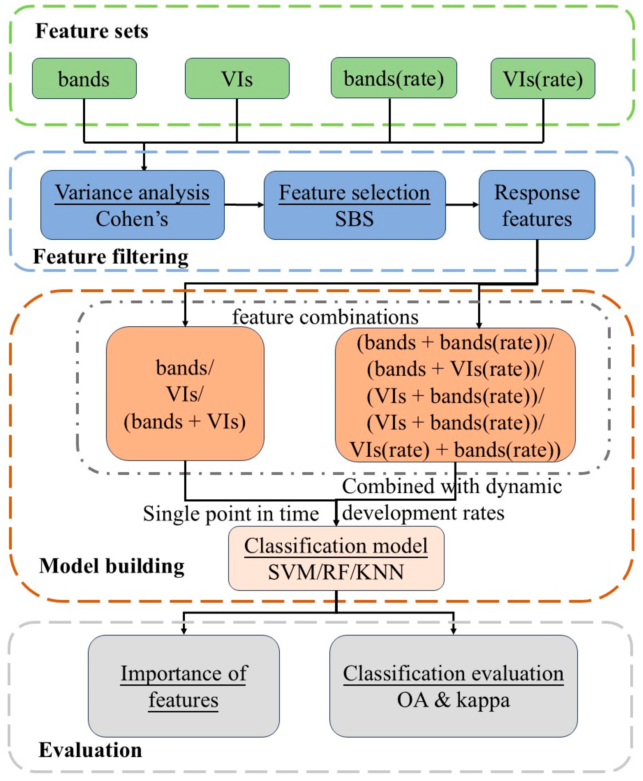
In this study, we introduced a method for resistance evaluation that incorporates the dynamic developmental rate of the disease (Figure 2). The process began by classifying the experimental points as tolerant or susceptible based on the resistance evaluation results. Subsequently, to evaluate the differences in hyperspectral features among cultivars with varying resistance levels during disease progression, as well as to assess the reliability of these features, we employed Cohen’s d as the primary statistical metric, with the p-value from independent samples t-tests used as a supporting indicator. An effect size threshold (d) was defined to determine whether a significant difference existed between tolerant and susceptible test sites. Based on a previous study [41], we considered |d| ≥ 0.8 and p < 0.05 as indicative of a statistically significant difference. Accordingly, we established a screening criterion for sensitive features: if a certain hyperspectral feature showed significant differences between varieties with different resistance levels across all time points, it was considered a temporal response feature for resistance evaluation and was retained for further analysis.
Resistance evaluation features were further screened and extracted using the Sequential Backward Selection (SBS) method. Prior to applying the SBS, features with greater robustness were preliminarily selected based on the confidence interval of Cohen’s d effect size (excluding zero). SBS is a feature selection method that starts with all features and iteratively removes the least important features one at a time until an optimal feature subset is identified. This approach has the advantage of eliminating redundant features and selecting the most representative set of features for resistance evaluation. Finally, a resistance assessment approach was established by integrating machine learning models with hyperspectral features from individual time points and disease progression rate features.

2.6. Model Construction Methods

To further validate the effectiveness of the selected features, we employed three classic classification models (Support Vector Machine [SVM], Random Forest [RF], and K-Nearest Neighbors [KNN]) and determined the final resistance evaluation model and hyperspectral features based on the results. SVM and RF exhibit significant potential for crop disease classification (achieving an accuracy of 99.04% for wheat yellow rust identification) [42,43].
Support Vector Machine (SVM): An SVM can handle linear and nonlinear problems. Using kernel functions to map data into a higher-dimensional space, problems are transformed into linearly separable forms. It identifies the optimal classification hyperplane by maximizing the classification margin, making it suitable for complex binary classification tasks.
Random Forest (RF): RF achieves classification by aggregating the votes of multiple decision trees. Each tree is trained on different subsets of data and features, thereby enhancing the generalization ability of the model. Owing to its randomness and diversity, the RF effectively avoids overfitting and improves model robustness, making it suitable for large-scale, high-noise binary classification problems.
K-Nearest Neighbors (KNN): KNN classifies samples based on the distance between data points and selects the K-Nearest Neighbors for voting. It is highly effective for handling nonlinear problems and does not require explicit model assumptions. Its simplicity and efficiency render it suitable for small-scale binary classification tasks.
Considering that the number of susceptible samples was smaller than that of tolerant samples, to address the class imbalance issue, the Synthetic Minority Over-sampling Technique (SMOTE) was applied to augment the number of susceptible samples. The dataset was divided into training and validation sets at a 4:1 ratio.
Model performance was assessed based on the confusion matrix, supplemented by key metrics: precision, recall, and the F1-score. Precision reflects the accuracy of positive predictions, recall measures the coverage of actual positives, and the F1-score balances the two. Together, they offer a detailed breakdown of classification efficacy. To further assess the generalization performance of the model on unseen data, we employed 10-fold cross-validation during the training process. This approach mitigates the influence of random data splits and provides a robust evaluation of model stability. Within each training fold of the cross-validation, hyperparameter optimization was systematically performed using GridSearchCV to identify the optimal parameter configuration [44]. This nested validation strategy ensures that the final model selection accurately represents generalized performance while maintaining strict separation between training and validation data throughout the tuning process.

3. Results

3.1. Temporal Variation Patterns of Physiological and Biochemical Parameters in Cotton Varieties with Different Resistance Levels During VW Progression

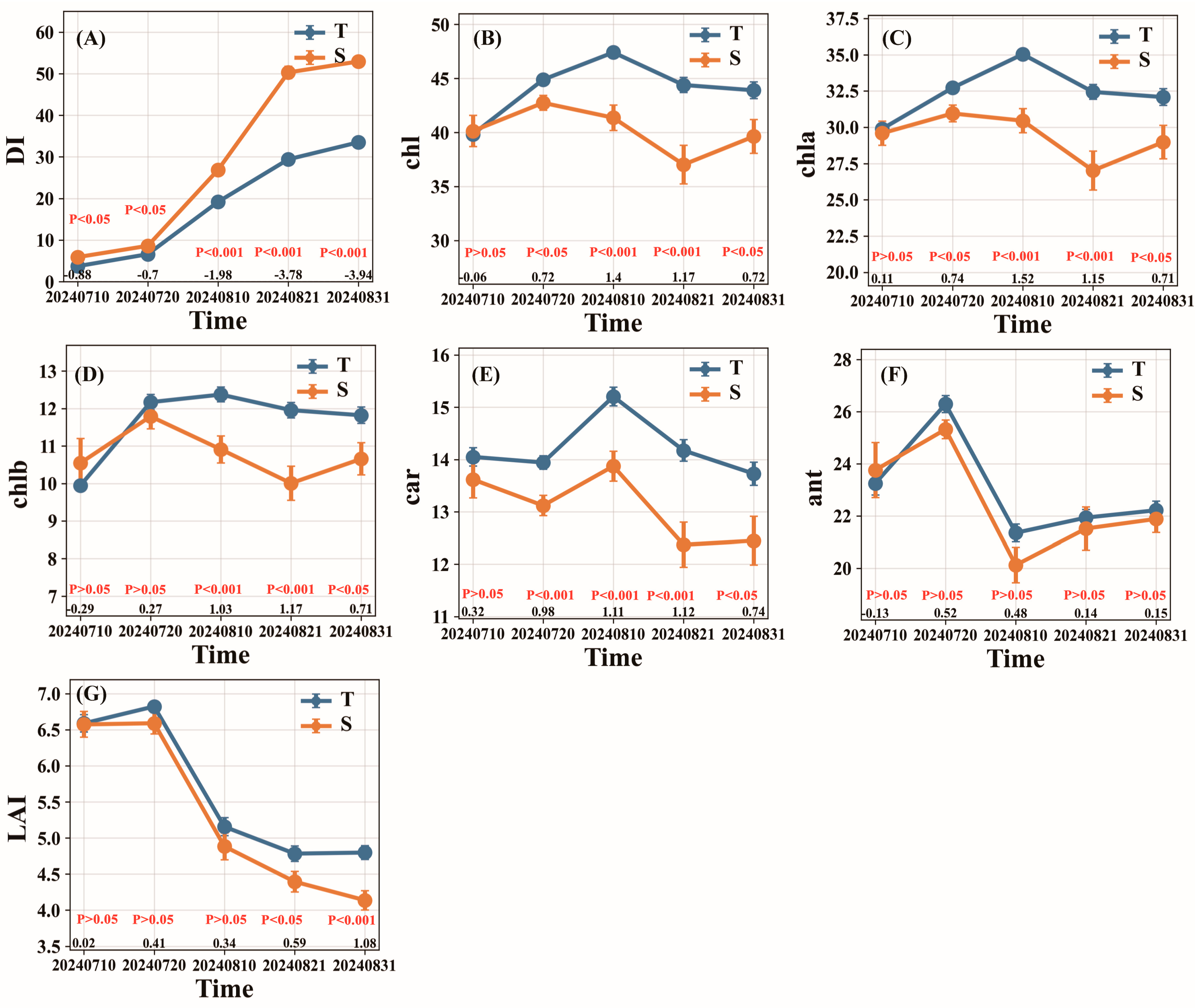
A significant difference analysis was conducted on the temporal leaf physiological traits and canopy structural characteristics of the different resistant varieties. During the progression of cotton VW, the disease index gradually increased in all cultivars, with tolerant cultivars consistently maintaining lower values, whereas susceptible varieties exhibited a more rapid and pronounced increase in DI over time (Figure 3A). All pigment contents exhibited an initial increase, subsequently decreasing (Figure 3B–F). Pigment accumulation in tolerant varieties continued to be higher than in susceptible varieties, starting from the flowering and boll stages (81 d after emergence). The chlorophyll content in the susceptible varieties began to decline 101 d after emergence, and this decline was delayed until 112 d in the tolerant varieties (Figure 3B–D). Differences in anthocyanin content were not significant throughout disease progression (Figure 3F). Although the leaf area index (LAI) exhibited a similar trend of an initial increase followed by a decrease in both varieties, and the LAI values of susceptible varieties were consistently lower than those of tolerant varieties, significant differences between them only appeared in the late stages of the experiment (Figure 3G).
Analysis of the disease progression rates revealed that the effects of resistance on the dynamic changes in physiological parameters exhibited apparent stage-specific characteristics (Table 3). Significant differences in the rate of disease index increase were observed throughout the infection process, except at the initial disease stage. During the mid-stage of disease development, susceptible cultivars showed a substantially faster increase in disease index than resistant cultivars. Overall, the degree of differentiation throughout the disease period was greater in the early stage (71–101 d after emergence) than in the later stage (101–122 d after emergence) ([|d| = 0.79] > [|d| = 0.47]). The overall rates of change in chlorophyll and carotenoid contents showed differences in resistance throughout the disease period (|d| > 0.2), whereas anthocyanins exhibited a differential response only in the initial stage of the disease (71–81 d after emergence). By the mid-disease stage (81–101 d after emergence), the difference in the overall rate of chlorophyll change remained moderate (d = 0.79). The difference in the rate of carotenoid change peaked at 101–112 d after emergence (d = 0.36), although it remained within a small range. In the final stage (112–122 d after emergence), the difference in chlorophyll a was the most significant (d = 0.47).

3.2. Temporal Hyperspectral Response Patterns of Cotton Varieties with Different Resistance Levels During VW Progression

3.2.1. Spectral Feature Response Based on Single Time-Phase

Within the 400–1030 nm wavelength range, spectral reflectance differences between varieties with different resistance levels initially appeared 81 d after emergence (Figure 4A–E), a time point synchronous with the significant differentiation stage of ground-based physiological parameters. Notably, the reflectance at 709 nm exhibited stable varietal differences starting 81 d after emergence (Figure 4F). Temporal difference analysis based on vegetation indices (Figure 5A–E) showed that the CIRed_edge index demonstrated significant varietal differences (d > 0.8) as early as 81 d after emergence, with its initial response time highly synchronized with changes in spectral reflectance. During the progression of disease stress, vegetation indices of varieties with different resistance levels exhibited dynamic response patterns: at 81 d after emergence, NDVI (pigment and structural index), HI, and CIRed_edge (red edge and photosynthetic physiological indices) responded simultaneously, with HI showing early resistance-sensitive characteristics; at 101 d after emergence, only CIRed_edge maintained significant differences; at 112 d after emergence, the responsive indices expanded to include CIRed_edge and five pigment and structural indices, MSR, MTVI, NDVI, OSAVI, and RDVI; and at 122 d after emergence, the sustained responses were limited to CIRed_edge, MSR, and NDVI, with NDVI demonstrating resistance differentiation capability at all monitoring time points except 101 d after emergence. Notably, CIRed_edge, as the only index responsive throughout the entire disease progression, exhibited excellent resistance sensitivity, while MSR also showed sustained differentiation capability during the late disease stage (101–122 d after emergence). Compared to the discrete responses of spectral reflectance, the regular changes in vegetation indices (particularly CIRed_edge and NDVI) across multiple time points were more conducive to constructing reliable resistance classification models.

3.2.2. Spectral Feature Response Based on Temporal Dynamic Development Rates

The differential analysis results of the dynamic development rates of spectral reflectance (Figure 6A–D, Table 4) showed that wavelengths with significant differences between resistance types existed only in the early disease stage (71–81 d after emergence). These significantly different wavelengths were concentrated at approximately 510 nm (characteristic green peak wavelength) and 680 nm (chlorophyll absorption valley). The varietal differences in change rates were more pronounced at approximately 680 nm (chlorophyll absorption valley) than at approximately 510 nm (characteristic green peak). Specifically, as disease severity increased, the spectral reflectance in these two wavelength ranges exhibited an upward trend, and the increase in reflectance of susceptible varieties during the early disease stage was significantly greater than that of the tolerant varieties (|d| > 0.8), resulting in negative values for significant differences.
Temporal analysis of vegetation indices further revealed that the early differences primarily resulted from the synergistic response of the red edge and photosynthetic physiological parameters (CIRed_edge index, d = 1.59) and pigment and structural parameters (PSSRc index, d = 1.40). In the mid-disease stage (81–101 d after emergence), although the chlorophyll content exhibited different trends (chl, d = 0.79), the declining trends of the canopy leaf area index converged (LAI, d = −0.01). This convergence persisted into the late disease stage, eliminating significant differences in the responses of the spectral vegetation indices (Figure 7A–D).

3.3. Results of Resistance Evaluation Models Based on Single-Time-Phase Spectral Features

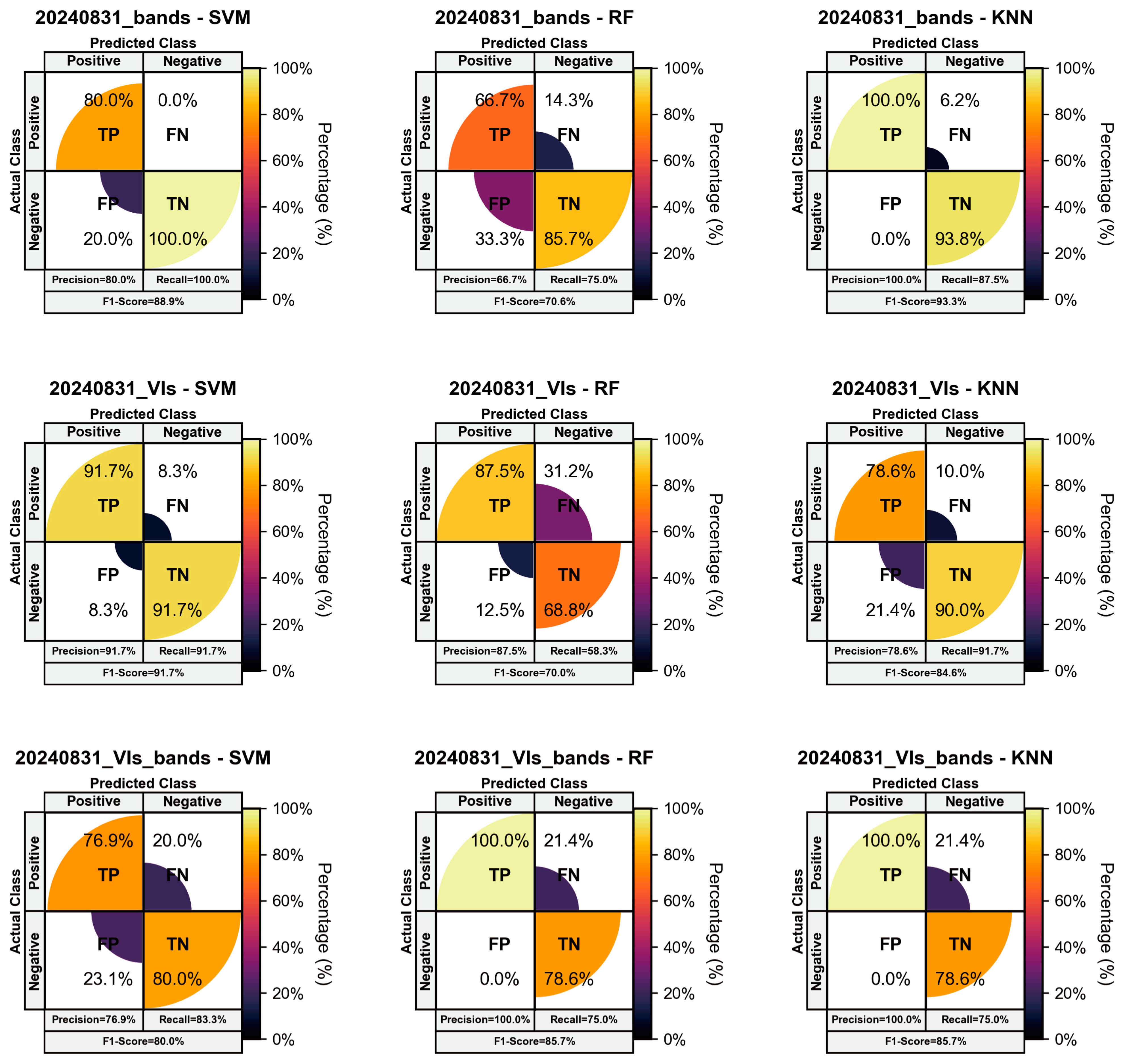
For the classification models, input variables included the temporally sensitive 709 nm wavelength and the CIRed_edge vegetation index, both derived from a single time point. We evaluated these features both individually and in combination across three models. Our comparative analysis identified that the overall optimal classification performance was achieved at 122 days after emergence, the results of which are presented in Figure 8, with the full set of classification results provided in Supplementary Materials Figure S1. On day 122 after emergence, using only the spectral band features with the KNN model yielded optimal classification performance, achieving a precision of 100%, a recall of 87.5%, and an F1-score of 93.3%. In contrast, during the early stages of the disease, the models exhibited a relatively weak ability to differentiate between samples with different resistance levels. Overall, when constructing the resistance evaluation models based on a single time point, the KNN model performed the best.

3.4. Results of Resistance Evaluation Models Incorporating Temporal Dynamic Development Rates

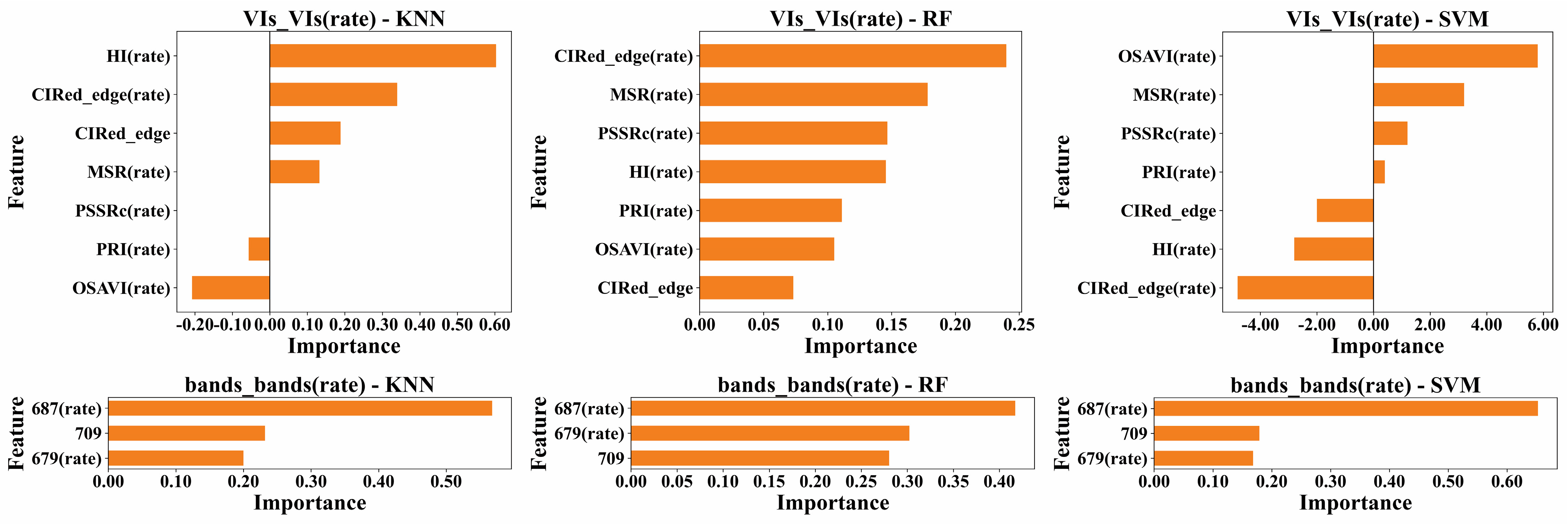
This study combined temporal features from a single time point in the early disease stage (71–81 d after emergence) with the dynamic developmental rate features of the corresponding time period. These features were input into three classification models in three forms: (1) vegetation index dynamic development rate features alone, (2) spectral reflectance dynamic development rate features alone, and (3) a combination of these dynamic development rate features with single-time-point temporal features. Based on the comparative analysis of the classification results, the optimal feature combination and its corresponding classification results are shown in Figure 9. The analysis results incorporating dynamic development rates indicated that during the early disease stage (71–81 d after emergence), when using spectral band reflectance (bands) and vegetation index dynamic development rates (VIs[rate]) with the KNN model for resistance evaluation, the model achieved a precision of 100%, recall of 66.7%, and F1-score of 80%. The complete set of classification results is available in Supplementary Materials Figure S2. Feature importance analysis (Figure 10) revealed that dynamic development rate features were critical in model performance.

4. Discussion

This study achieved efficient resistance evaluation of cotton varieties with diverse genotypes at a single time point through the integration of UAV-based hyperspectral technology and machine learning, demonstrating strong predictive performance. In this study, we compared the effectiveness of resistance evaluation based on spectral features at different time points and identified the optimal evaluation period. The spectral features at 709 nm and CIRed_edge exhibited significant differences between the resistant and susceptible varieties throughout the various stages of cotton VW progression. Ground-measured leaf pigments, particularly chlorophyll, also showed temporal variation. This phenomenon is closely related to the optical characteristics of the spectral red-edge region (680–750 nm), which results from the synergistic interaction between efficient chlorophyll absorption in the red region and multiple scattering by cellular structures in the near-infrared region. This phenomenon is susceptible to the physiological status of crops, exhibiting characteristic shifts or distortions in response to variations in chlorophyll content, nitrogen levels, and biomass [45]. Particularly under disease stress, alterations in leaf biochemical components and cellular structure result in notable changes in red-edge parameters [46]. Chen et al. [11] demonstrated that both chlorophyll and nitrogen content in diseased cotton leaves were significantly positively correlated with red-edge parameters. Ref. [47] demonstrated that the red-edge index was significantly influenced by the chlorophyll content in leaves. The red-edge index has been extensively used to identify abiotic stress conditions that significantly affect leaf pigment concentrations [48,49]. Based on ground-measured pigment data, we observed that the chlorophyll content in tolerant varieties consistently remained higher than that in susceptible varieties under VW stress, with temporal differences further indicating that chlorophyll content is a sensitive physiological indicator of resistance. The red-edge region features were identified as key spectral characteristics for differentiating varieties with different resistance levels. However, resistance evaluation based on spectral features combined with machine learning models only achieved satisfactory results in the late disease stage, with limited ability to differentiate resistance in the early stage. This phenomenon is closely related to the pathological characteristics of Verticillium wilt: significant differences in the red-edge region and the 680 nm absorption trough only became apparent after pigment levels had declined beyond a certain threshold. During the early stages of VW stress, asymptomatic leaves exhibited minimal pigment degradation, resulting in limited impact on the spectral bands. Differentiation increases primarily in the later stages, when chlorophyll degrades substantially and symptoms become evident [16,50]. Thus, the pigment content contributes minimally to the mild stage of the disease. UAV-based monitoring primarily captures spectral information from the upper canopy leaves. However, Verticillium wilt develops from the bottom up, and in the early stages of infection, the upper leaves typically show no visible symptoms, making remote sensing-based detection relatively difficult [9]. This also explains the suboptimal performance of resistance evaluation in the early disease stages observed in this study.
The key innovation of this study is the introduction of temporal dynamic analysis. By quantifying the rate of change in spectral features during the flowering stage (71–81 d after emergence), the accuracy of resistance assessment was improved to 0.84 (kappa = 0.68). The calculation of the disease development rate is based on analyzing temporal variations in spectral features derived from time-series data. This method quantifies the rate of change in spectral parameters between adjacent observation time points and correlates them with crop disease progression, thereby enabling the scientific characterization of the disease development rate. This time-dynamic analytical approach effectively integrates spatiotemporal variations in spectral responses, revealing dynamic evolutionary patterns during pathogen infection. For instance, considering early disease development (71–81 d after emergence) at the initial time point (71 d after emergence), the spectral characteristics of varieties with different resistance levels were similar, making it difficult to distinguish them based on a single time point. However, by 81 d after emergence, considerably different wavelengths were primarily concentrated at approximately 500–600 and 700 nm. Notably, in the 500–600 nm range, the reflectance of tolerant varieties was significantly lower than that of susceptible varieties. This phenomenon indicates that as disease severity increases, reflectance in the 500–600 nm band tends to increase, but the increase is significantly smaller in tolerant varieties than in susceptible ones. The key finding is that the rate of spectral change based on temporal dynamics provides greater discriminatory power than features from a single time point. Although spectral data at 81 d after emergence alone were insufficient to effectively distinguish varietal resistance, by calculating the rate of change (the increase) in key spectral features (reflectance at 500–600 nm) from days 71 to 81 and analyzing them using machine learning models, we effectively achieved high-precision classification of varietal resistance (with optimal accuracy reaching 84%). The rate of change in spectral features sensitively indicates the actual differences in disease progression rates among varieties with different resistance levels, thereby indicating their inherent disease resistance capability. Based on feature importance analysis, 687 nm and CIRed_edge were identified as key dynamic development rate features for early-stage resistance evaluation, showing strong consistency with the critical resistance evaluation features from single time points. This further indicates that chlorophyll is a key sensitive indicator for resistance evaluation and that canopy structure significantly influences canopy pigments. Chlorophyll is the primary pigment responsible for photosynthesis and organic nutrient accumulation in green plants, and its content determines the strength of photosynthetic activity. Thus, chlorophyll is closely related to plant growth capacity [51,52]. In soybean breeding programs targeting high photosynthetic rates, chlorophyll content measurements can be used for preliminary screening of progeny [53]. During the early stages of cotton Verticillium wilt, genes associated with lignin synthesis are expressed to strengthen cell walls and structures, thereby enhancing resistance [54]. Additionally, during stress conditions, the trend of chlorophyll content changes in crop leaves is similar to that of lignin content [55,56]. This suggests that varieties with varying resistance levels regulate the expression of lignin synthesis genes in the early stages of disease to influence chlorophyll accumulation in canopy leaves, with tolerant varieties accumulating more chlorophyll than susceptible varieties, which is consistent with our findings. The chlorophyll content exhibited close correlation with the spectral features in the red-edge region. The red-edge characteristics of the tolerant varieties differed considerably from those of the susceptible varieties, indicating that the red-edge region also has discriminatory power in the early disease stage. However, differences based on a single time point are insufficient for reliable resistance evaluation, whereas incorporating dynamic development rates enables effective resistance assessment during early disease stages. By capturing the rate of spectral change during the early stages of disease, our approach provides a critical time period for early screening in resistance breeding. This enables precise identification of resistant lines at the pre-symptomatic stage, which is expected to shorten the breeding cycle.
Although this study presents valuable findings, there are opportunities for further advancements in future research. The current analysis was limited to a specific set of cotton cultivars; therefore, expanding the evaluation to include a broader range of germplasm, particularly materials with higher resistance levels, would enhance the validation of the wider applicability of the methodology. Additionally, although the model demonstrated robust performance under cross-validation, its stability across different growing seasons and geographical regions could be further validated through multi-year, multi-location trials. A potential area for future research involves establishing quantitative links between the dynamic resistance characteristics identified in this study and final yield outcomes, which would strengthen the practical utility of the evaluation framework. Further integration of multi-source remote sensing data and exploration of temporal relationships between spectral features and yield formation would also contribute to developing a more comprehensive resistance monitoring system.

5. Conclusions

In this study, we developed a novel method for assessing cotton resistance to Verticillium wilt by integrating temporal remote sensing features with disease progression rates. The results demonstrated that traditional approaches relying solely on canopy spectral data from a single time point were limited in early-stage disease detection. In contrast, incorporating dynamic change rate features significantly improved early resistance identification, achieving a precision of 100%, a recall of 66.7%, and an F1-Score of 80%. Notably, resistance differentiation was successfully achieved as early as 81 d after emergence. The 709 nm spectral band and the CIRed_edge were identified as key features for differentiating resistant and susceptible cultivars. This study provides a time-series-based remote sensing approach for evaluating resistance to Verticillium wilt in cotton, offering valuable support for resistance breeding practices. Future research may further explore the relationship between early disease progression rates and cotton yield formation to refine resistance evaluation systems and advance the precision breeding of disease-resistant cultivars through both theoretical insight and technical support.

Supplementary Materials

The following supporting information can be downloaded at: https://www.mdpi.com/article/10.3390/rs17223701/s1, Figure S1: Classification results of resistance assessment models based on single-time-phase spectral features. Figure S2: Classification results of resistance assessment models incorporating temporal dynamic development rate features.

Author Contributions

Conceptualization, J.W. and M.Y.; methodology, J.W., M.Y., Y.G. and J.Z.; validation, J.W., M.Y. and Z.Z. (Ze Zhang); formal analysis, J.W.; investigation, Z.Z. (Ze Zhang); resources, C.H., Z.Z. (Ze Zhang) and Z.Z. (Zhihong Zheng); data curation, J.W., C.Z., M.G. and L.Z.; writing—original draft preparation, J.W. and M.Y.; writing—review and editing, C.H., Z.Z. (Ze Zhang) and J.W.; visualization, J.W. and C.Z.; supervision, Z.Z. (Ze Zhang) and C.H.; project administration, Z.Z. (Ze Zhang) and C.H.; funding acquisition, Z.Z. (Ze Zhang) and C.H. All authors have read and agreed to the published version of the manuscript.

Funding

This study was supported by the Major projects in the Corps, including the Smart Breeding Project for Corps Cotton Research on Corps Cotton Breeding AI Model [No. 2023AA008], Key Projects of the Corps Science and Technology (No. 2025DA007), National Natural Science Foundation of China (No. 42571423), and the Corps Leading Talent Project, Eighth Division Shihezi City Mid-Aged and Young Scientific and Technological Innovation Backbone Talent Program Project (No. 2024RC01).

Data Availability Statement

Data are contained within the article and Supplementary Materials.

Conflicts of Interest

The authors declare that the research was conducted in the absence of any commercial or financial relationships that could be construed as a potential conflict of interest.

Abbreviations

The following abbreviations are used in this manuscript:
DIDisease index
ARDIAverage relative disease index
DCNNDeep convolutional neural networks
DNDigital number
DTSMDecision Tree-based Segmentation Model
DW Dry weight
KNNK-Nearest Neighbors
LAILeaf area index
LWCLeaf water content
OAOverall accuracy
RFRandom Forest
ROIRegions of interest
SBSSequential Backward Selection
SEMStandard errors
SVMSupport Vector Machine
UAVUnmanned aerial vehicle
VWVerticillium wilt

References

  1. Fradin, E.F.; Thomma, B.P.H.J. Physiology and Molecular Aspects of Verticillium Wilt Diseases Caused by V. dahliae and V. albo-atrum. Mol. Plant Pathol. 2006, 7, 71–86. [Google Scholar] [CrossRef]
  2. Zhang, D.; Wang, J.; Wang, D.; Kong, Z.; Zhou, L.; Zhang, G.; Gui, Y.; Li, J.; Huang, J.; Wang, B.; et al. Population Genomics Demystifies the Defoliation Phenotype in the Plant Pathogen Verticillium dahliae. New Phytol. 2019, 222, 1012–1029. [Google Scholar] [CrossRef]
  3. Zhang, Y.; Yuan, Y.; Xi, H.; Zhang, Y.; Gao, C.; Ma, M.; Huang, Q.; Li, F.; Yang, Z. Promotion of Apoplastic Oxidative Burst by Artificially Selected GhCBSX3A Enhances Verticillium dahliae Resistance in Upland Cotton. Plant J. 2024, 118, 2154–2168. [Google Scholar] [CrossRef] [PubMed]
  4. Shaban, M.; Miao, Y.; Ullah, A.; Khan, A.Q.; Menghwar, H.; Khan, A.H.; Ahmed, M.M.; Tabassum, M.A.; Zhu, L. Physiological and Molecular Mechanism of Defense in Cotton against Verticillium dahliae. Plant Physiol. Biochem. 2018, 125, 193–204. [Google Scholar] [CrossRef] [PubMed]
  5. Kowalska, B. Management of the Soil-Borne Fungal Pathogen— Verticillium dahliae Kleb. Causing Vascular Wilt Diseases. J. Plant Pathol. 2021, 103, 1185–1194. [Google Scholar] [CrossRef]
  6. Yin, X.; Zou, B.; Hong, X.; Gao, M.; Yang, W.; Zhong, X.; He, Y.; Kuai, P.; Lou, Y.; Huang, J.; et al. Rice Copine Genes Os BON 1 and Os BON 3 Function as Suppressors of Broad-spectrum Disease Resistance. Plant Biotechnol. J. 2018, 16, 1476–1487. [Google Scholar] [CrossRef]
  7. Da Graça, J.V.; Douhan, G.W.; Halbert, S.E.; Keremane, M.L.; Lee, R.F.; Vidalakis, G.; Zhao, H. Huanglongbing: An Overview of a Complex Pathosystem Ravaging the World’s Citrus. J. Integr. Plant Biol. 2016, 58, 373–387. [Google Scholar] [CrossRef]
  8. Bai, Y.; Zarco-Tejada, P.J.; Peñuelas, J.; McCabe, M.F.; Hawkesford, M.J.; Atzberger, C.; Poblete, T.; Kumar, L.; Reynolds, M.P.; Nie, C.; et al. Hyperspectral Remote Sensing for Monitoring Crop Disease: Applications, Challenges, and Perspectives. IEEE Geosci. Remote Sens. Mag. 2025, 2–26. [Google Scholar] [CrossRef]
  9. Gui, Y.; Huang, C.; Zhou, J.; Yang, M.; Qiu, X.; Zhang, Z.; Liu, Y.; Gao, Y.; Shen, W.; Huang, W.; et al. A Practical Approach for Grading Cotton Verticillium Wilt Severity for Remote Sensing Monitoring. Agric. For. Meteorol. 2025, 368, 110559. [Google Scholar] [CrossRef]
  10. Mishra, P.; Polder, G.; Vilfan, N. Close Range Spectral Imaging for Disease Detection in Plants Using Autonomous Platforms: A Review on Recent Studies. Curr. Robot. Rep. 2020, 1, 43–48. [Google Scholar] [CrossRef]
  11. Chen, B.; Han, H.-Y.; Wang, F.-Y.; Liu, Z.; Deng, F.-J.; Lin, H.; Yu, Y.; Li, S.-K.; Wang, K.-R.; Xiao, C.-H. Monitoring Chlorophyll and Nitrogen Contents in Cotton Leaf Infected by Verticillium wilt with Spectra Red Edge Parameters. Acta Agron. Sin. 2013, 39, 319. [Google Scholar] [CrossRef]
  12. Zhang, Y.; Chen, B.; Sun, Z.; Liu, Z.; Cui, Y.; Ke, H.; Wang, Z.; Wu, L.; Zhang, G.; Wang, G.; et al. A Large-scale Genomic Association Analysis Identifies a Fragment in Dt11 Chromosome Conferring Cotton Verticillium Wilt Resistance. Plant Biotechnol. J. 2021, 19, 2126–2138. [Google Scholar] [CrossRef]
  13. Kang, X. Assessing the Severity of Cotton Verticillium Wilt Disease from in Situ Canopy Images and Spectra Using Convolutional Neural Networks. Crop J. 2023, 11, 933–940. [Google Scholar] [CrossRef]
  14. Zhao, L. Development of an Improved Standard for Identifying and Evaluating Verticillium Wilt Resistance in Cotton. Cotton Sci. 2017, 29, 50–58. [Google Scholar] [CrossRef]
  15. Calderón, R.; Navas-Cortés, J.A.; Lucena, C.; Zarco-Tejada, P.J. High-Resolution Airborne Hyperspectral and Thermal Imagery for Early Detection of Verticillium Wilt of Olive Using Fluorescence, Temperature and Narrow-Band Spectral Indices. Remote Sens. Environ. 2013, 139, 231–245. [Google Scholar] [CrossRef]
  16. Yang, M.; Huang, C.; Kang, X.; Qin, S.; Ma, L.; Wang, J.; Zhou, X.; Lv, X.; Zhang, Z. Early Monitoring of Cotton Verticillium Wilt by Leaf Multiple “Symptom” Characteristics. Remote Sens. 2022, 14, 5241. [Google Scholar] [CrossRef]
  17. Weng, H.; Yao, Y.; Huang, D. Rapid Evaluation of Rice Neck Blast Resistance Using Low Altitude Remote Sensing of UAV Combined with YOLOv7. Trans. Chin. Soc. Agric. Eng. 2024, 40, 110–118. [Google Scholar]
  18. Liu, T.; Qi, Y.; Yang, F.; Yi, X.; Guo, S.; Wu, P.; Yuan, Q.; Xu, T. Early Detection of Rice Blast Using UAV Hyperspectral Imagery and Multi-Scale Integrator Selection Attention Transformer Network (MS-STNet). Comput. Electron. Agric. 2025, 231, 110007. [Google Scholar] [CrossRef]
  19. Hu, J.; Huang, J.; Xu, H.; Wang, Y.; Li, C.; Wen, P.; You, X.; Zhang, X.; Pan, G.; Li, Q.; et al. Rice Stripe Virus Suppresses Jasmonic Acid-Mediated Resistance by Hijacking Brassinosteroid Signaling Pathway in Rice. PLoS Pathog. 2020, 16, e1008801. [Google Scholar] [CrossRef]
  20. Xia, Z.; Achar, P.N.; Gu, B. Vegetative Compatibility Groupings of Verticillium dahliae from Cotton in Mainland China. Eur. J. Plant Pathol. 1998, 104, 871–876. [Google Scholar] [CrossRef]
  21. Jiang, Z.; Tu, H.; Bai, B.; Yang, C.; Zhao, B.; Guo, Z.; Liu, Q.; Zhao, H.; Yang, W.; Xiong, L.; et al. Combining UAV-RGB High-throughput Field Phenotyping and Genome-wide Association Study to Reveal Genetic Variation of Rice Germplasms in Dynamic Response to Drought Stress. New Phytol. 2021, 232, 440–455. [Google Scholar] [CrossRef]
  22. Han, L.; Yang, G.; Yang, H.; Xu, B.; Li, Z.; Yang, X. Clustering Field-Based Maize Phenotyping of Plant-Height Growth and Canopy Spectral Dynamics Using a UAV Remote-Sensing Approach. Front. Plant Sci. 2018, 9, 1638. [Google Scholar] [CrossRef]
  23. Xie, Z.; Chen, S.; Gao, G.; Li, H.; Wu, X.; Meng, L.; Ma, Y. Evaluation of Rapeseed Flowering Dynamics for Different Genotypes with UAV Platform and Machine Learning Algorithm. Precis. Agric. 2022, 23, 1688–1706. [Google Scholar] [CrossRef]
  24. Zhou, J.; Huang, C.; Gui, Y.; Yang, M.; Zhang, Z.; Huang, W.; Zhang, L.; Tong, Q. Roles of Physiological and Nonphysiological Information in Sun-Induced Chlorophyll Fluorescence Variations for Detecting Cotton Verticillium Wilt. IEEE J. Sel. Top. Appl. Earth Obs. Remote Sens. 2024, 17, 8835–8850. [Google Scholar] [CrossRef]
  25. NY/T 2952-2016; Technical Specification for Identification of Cotton Verticillium Wilt Resistance. China Agriculture Press: Beijing, China, 2016.
  26. Pearse, G.D.; Watt, M.S.; Morgenroth, J. Comparison of Optical LAI Measurements under Diffuse and Clear Skies after Correcting for Scattered Radiation. Agric. For. Meteorol. 2016, 221, 61–70. [Google Scholar] [CrossRef]
  27. Murray, J.R.; Hackett, W.P. Dihydroflavonol Reductase Activity in Relation to Differential Anthocyanin Accumulation in Juvenile and Mature Phase Hedera helix L. Plant Physiol. 1991, 97, 343–351. [Google Scholar] [CrossRef] [PubMed]
  28. Hornero, A.; Zarco-Tejada, P.J.; Quero, J.L.; North, P.R.J.; Ruiz-Gómez, F.J.; Sánchez-Cuesta, R.; Hernandez-Clemente, R. Modelling Hyperspectral- and Thermal-Based Plant Traits for the Early Detection of Phytophthora-Induced Symptoms in Oak Decline. Remote Sens. Environ. 2021, 263, 112570. [Google Scholar] [CrossRef]
  29. Ishiyama, T.; Nakajima, Y.; Kajiwara, K.; Tsuchiya, K. Extraction of Vegetation Cover in an Arid Area Based on Satellite Data. Adv. Space Res. 1997, 19, 1375–1378. [Google Scholar] [CrossRef]
  30. Roujean, J.-L.; Breon, F.-M. Estimating PAR Absorbed by Vegetation from Bidirectional Reflectance Measurements. Remote Sens. Environ. 1995, 51, 375–384. [Google Scholar] [CrossRef]
  31. Chen, J.M. Evaluation of Vegetation Indices and a Modified Simple Ratio for Boreal Applications. Can. J. Remote Sens. 1996, 22, 229–242. [Google Scholar] [CrossRef]
  32. Rondeaux, G.; Steven, M.; Baret, F. Optimization of Soil-Adjusted Vegetation Indices. Remote Sens. Environ. 1996, 55, 95–107. [Google Scholar] [CrossRef]
  33. Haboudane, D.; Miller, J.R.; Tremblay, N.; Zarco-Tejada, P.J.; Dextraze, L. Integrated Narrow-Band Vegetation Indices for Prediction of Crop Chlorophyll Content for Application to Precision Agriculture. Remote Sens. Environ. 2002, 81, 416–426. [Google Scholar] [CrossRef]
  34. Haboudane, D. Hyperspectral Vegetation Indices and Novel Algorithms for Predicting Green LAI of Crop Canopies: Modeling and Validation in the Context of Precision Agriculture. Remote Sens. Environ. 2004, 90, 337–352. [Google Scholar] [CrossRef]
  35. Blackburn, G.A. Spectral Indices for Estimating Photosynthetic Pigment Concentrations: A Test Using Senescent Tree Leaves. Int. J. Remote Sens. 1998, 19, 657–675. [Google Scholar] [CrossRef]
  36. Penuelas, J.; Pinol, J.; Ogaya, R.; Filella, I. Estimation of Plant Water Concentration by the Reflectance Water Index WI (R900/R970). Int. J. Remote Sens. 1997, 18, 2869–2875. [Google Scholar] [CrossRef]
  37. Mahlein, A.-K.; Rumpf, T.; Welke, P.; Dehne, H.-W.; Plümer, L.; Steiner, U.; Oerke, E.-C. Development of Spectral Indices for Detecting and Identifying Plant Diseases. Remote Sens. Environ. 2013, 128, 21–30. [Google Scholar] [CrossRef]
  38. Gitelson, A.A.; Gritz, Y.; Merzlyak, M.N. Relationships between Leaf Chlorophyll Content and Spectral Reflectance and Algorithms for Non-Destructive Chlorophyll Assessment in Higher Plant Leaves. J. Plant Physiol. 2003, 160, 271–282. [Google Scholar] [CrossRef]
  39. Gamon, J.A.; Peñuelas, J.; Field, C.B. A Narrow-Waveband Spectral Index That Tracks Diurnal Changes in Photosynthetic Efficiency. Remote Sens. Environ. 1992, 41, 35–44. [Google Scholar] [CrossRef]
  40. Ma, Y.; Zhang, Q.; Yi, X.; Ma, L.; Zhang, L.; Huang, C.; Zhang, Z.; Lv, X. Estimation of Cotton Leaf Area Index (LAI) Based on Spectral Transformation and Vegetation Index. Remote Sens. 2021, 14, 136. [Google Scholar] [CrossRef]
  41. Yang, P.; van der Tol, C.; Liu, J.; Liu, Z. Separation of the Direct Reflection of Soil from Canopy Spectral Reflectance. Remote Sens. Environ. 2025, 316, 114500. [Google Scholar] [CrossRef]
  42. Shahi, T.B.; Xu, C.-Y.; Neupane, A.; Guo, W. Recent Advances in Crop Disease Detection Using UAV and Deep Learning Techniques. Remote Sens. 2023, 15, 2450. [Google Scholar] [CrossRef]
  43. Yuan, L.; Yu, Q.; Xiang, L.; Zeng, F.; Dong, J.; Xu, O.; Zhang, J. Integrating UAV and High-Resolution Satellite Remote Sensing for Multi-Scale Rice Disease Monitoring. Comput. Electron. Agric. 2025, 234, 110287. [Google Scholar] [CrossRef]
  44. Cai, A.; Wang, L.; Zhang, Y.; Wu, H.; Zhang, H.; Guo, R.; Wu, J. Uncovering the Multiple Socio-Economic Driving Factors of Carbon Emissions in Nine Urban Agglomerations of China Based on Machine Learning. Energy 2025, 319, 134859. [Google Scholar] [CrossRef]
  45. Smith, K.L.; Steven, M.D.; Colls, J.J. Use of Hyperspectral Derivative Ratios in the Red-Edge Region to Identify Plant Stress Responses to Gas Leaks. Remote Sens. Environ. 2004, 92, 207–217. [Google Scholar] [CrossRef]
  46. Chen, B.; Li, S.; Wang, K.; Zhou, G.; Bai, J. Evaluating the Severity Level of Cotton Verticillium Using Spectral Signature Analysis. Int. J. Remote Sens. 2012, 33, 2706–2724. [Google Scholar] [CrossRef]
  47. Li, W.; Li, D.; Warner, T.A.; Liu, S.; Baret, F.; Yang, P.; Jiang, J.; Dong, M.; Cheng, T.; Zhu, Y.; et al. Improved Generality of Wheat Green LAI Models through Mitigation of the Effect of Leaf Chlorophyll Content Variation with Red Edge Vegetation Indices. Remote Sens. Environ. 2025, 318, 114589. [Google Scholar] [CrossRef]
  48. Zhang, L.; Qiao, N.; Huang, C.; Wang, S. Monitoring Drought Effects on Vegetation Productivity Using Satellite Solar-Induced Chlorophyll Fluorescence. Remote Sens. 2019, 11, 378. [Google Scholar] [CrossRef]
  49. Ortiz, J.C.M.; Carvajal, L.M.H.; Fernandez, V.B. Detection of Significant Wavelengths for Identifying and Classifying Fusarium Oxysporum during the Incubation Period and Water Stress in Solanum Lycopersicum Plants Using Reflectance Spectroscopy. J. Plant Prot. Res. 2019, 59. [Google Scholar] [CrossRef]
  50. Tzeng, D.D.; De Vay, J.E. Physiological Responses of Gossypium Hirsutum L. to Infection by Defoliating and Nondefoliating Pathotypes of Verticillium dahliae Kleb. Physiol. Plant Pathol. 1985, 26, 57–72. [Google Scholar] [CrossRef]
  51. Croft, H.; Chen, J.M.; Luo, X.; Bartlett, P.; Chen, B.; Staebler, R.M. Leaf Chlorophyll Content as a Proxy for Leaf Photosynthetic Capacity. Glob. Change Biol. 2017, 23, 3513–3524. [Google Scholar] [CrossRef]
  52. Anderson, M.C. Photon Flux, Chlorophyll Content, and Photosynthesis Under Natural Conditions. Ecology 1967, 48, 1050–1053. [Google Scholar] [CrossRef]
  53. Buttery, B.R.; Buzzell, R.I. The Relationship Between Chlorophyll Content and Rate of Photosynthesis in Soybeans. Can. J. Plant Sci. 1977, 57, 1–5. [Google Scholar] [CrossRef]
  54. Qiu, P.; Li, J.; Zhang, L.; Chen, K.; Shao, J.; Zheng, B.; Yuan, H.; Qi, J.; Yue, L.; Hu, Q.; et al. Polyethyleneimine-Coated MXene Quantum Dots Improve Cotton Tolerance to Verticillium dahliae by Maintaining ROS Homeostasis. Nat. Commun. 2023, 14, 7392. [Google Scholar] [CrossRef] [PubMed]
  55. Yuan, L.; Dang, J.; Zhang, J.; Wang, L.; Zheng, H.; Li, G.; Li, J.; Zhou, F.; Khan, A.; Zhang, Z.; et al. A Glutathione S-Transferase Regulates Lignin Biosynthesis and Enhances Salt Tolerance in Tomato. Plant Physiol. 2024, 196, 2989–3006. [Google Scholar] [CrossRef] [PubMed]
  56. Li, Y.-P.; Su, L.-Y.; Huang, T.; Liu, H.; Tan, S.-S.; Deng, Y.-J.; Wang, Y.-H.; Xiong, A.-S. The Telomere-to-Telomere Genome of Pucai (Typha angustifolia L.), a Distinctive Semi-Aquatic Vegetable with Lignin and Chlorophyll as Quality Characteristics. Hortic. Res. 2025, 12, uhaf079. [Google Scholar] [CrossRef]
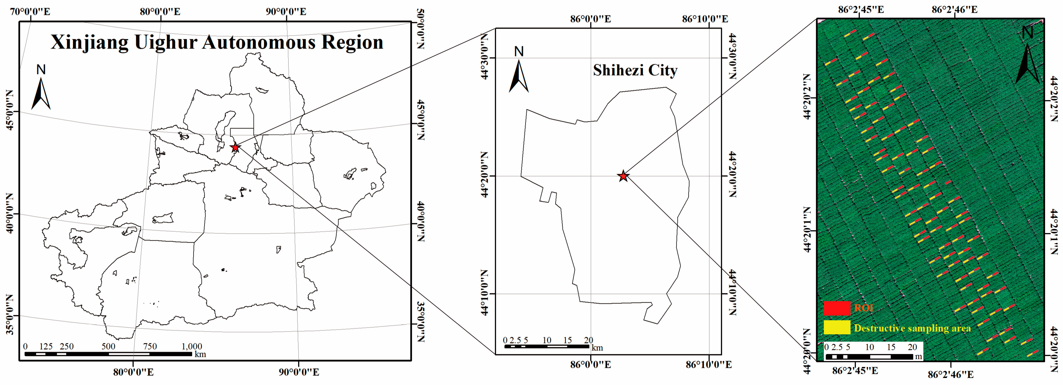
Figure 1. Location of the study area and the experimental design. The regions of interest (ROIs) and destructive sampling areas are indicated. Destructive sampling was consistently conducted on the left side of each plot to minimize interference with the canopy area dedicated to time-series spectral monitoring. Considering that all cultivars were planted under identical management practices and pathogen distribution was relatively uniform across each plot, the population structure was considered homogeneous between the left and right sides. Therefore, samples collected from the left side are representative.
Remotesensing 17 03701 g001
Figure 2. Overview of the methodology for resistance evaluation incorporating the dynamic development rate of the disease. Note: bands, spectral reflectance at specific wavelengths; VIs, Vegetation Indices; bands(rate), rate of change in spectral reflectance; VIs(rate), rate of change in Vegetation Indices; SBS, Sequential Backward Selection algorithm; SVM, Support Vector Machine classification model; RF, Random Forest classification model; KNN, K-Nearest Neighbors classification model.
Remotesensing 17 03701 g002
Figure 3. Panel (A) shows the temporal changes in disease index during the progression of cotton Verticillium wilt for tolerant (n = 60) and susceptible (n = 20) varieties. Panels (BG) present the corresponding temporal changes in physiological and biochemical parameters. Error bars represent a 95% confidence interval, with numerical values indicating the effect size as determined by Cohen’s d. T, Tolerant varieties; S, Susceptible varieties; DI, disease index; chl, chlorophyll a + b content; chla, chlorophyll a content; chlb, chlorophyll b content; car, carotenoid content; ant, anthocyanin content; LAI, leaf area index. p-values were obtained using independent t-tests conducted between tolerant and susceptible varieties at each time point.
Remotesensing 17 03701 g003
Figure 4. Spectral reflectance at 400–1030 nm for tolerant (n = 60) and susceptible (n = 20) cotton varieties during Verticillium wilt progression (AE). Each panel shows the original mean reflectance spectra alongside the corresponding effect size (absolute value of Cohen’s d) quantifying differences between variety groups. An absolute effect size value ≥ 0.8 combined with p < 0.05 is considered statistically significant between the two groups. The error band represents the 95% confidence interval. Reflectance at 709 nm exhibited stable and significant differences between varieties, starting 81 d after emergence (20240720) (F).
Remotesensing 17 03701 g004
Figure 5. Vegetation indices differentiating tolerant (n = 60) and susceptible (n = 20) varieties during the progression of cotton VW (AE). Each data point represents the effect size of the differences between tolerant and susceptible varieties. An absolute effect size value ≥ 0.8 combined with p < 0.05 is considered statistically significant between the two groups, and these significant differences are highlighted in red. Error bars represent 95% confidence intervals. CIRed_edge exhibited stable and significant differences between varieties, starting 81 d after emergence (20240720).
Remotesensing 17 03701 g005
Figure 6. Rate of change in spectral reflectance at 400–1030 nm differentiating tolerant (n = 60) and susceptible (n = 20) varieties during the progression of cotton VW (AD). Each data point represents the effect size of differences between tolerant and susceptible varieties. An absolute effect size value ≥ 0.8 is considered statistically significant between the two groups. An absolute effect size value ≥ 0.8 combined with p < 0.05 is considered statistically significant between the two groups. The error band represents the 95% confidence interval.
Remotesensing 17 03701 g006
Figure 7. Vegetation indices differentiating tolerant varieties (n = 60) and susceptible (n = 20) varieties during the progression of cotton VW (AD). Each data point represents the effect size of the differences between tolerant and susceptible varieties. An absolute effect size value ≥ 0.8 combined with p < 0.05 is considered statistically significant between the two groups. Error bars represent the 95% confidence interval.
Remotesensing 17 03701 g007
Figure 8. Detailed classification results at the optimal time point, presenting Precision, Recall, and F1-score for three classifiers (SVM, RF, and KNN) trained on spectral bands (bands), vegetation indices (VIs), and their combination (VIs_bands). Each quadrant represents a component of the confusion matrix, providing an intuitive comparison of classification effectiveness across feature sets.
Remotesensing 17 03701 g008
Figure 9. Detailed classification results based on the feature combination incorporating dynamic change rates (bands_VIs[rate]), presenting Precision, Recall, and F1-score for three classifiers (SVM, RF, and KNN). Each quadrant represents a component of the confusion matrix, providing an intuitive visualization of the classification performance under this optimal feature set.
Remotesensing 17 03701 g009
Figure 10. Feature importance scores incorporating disease dynamic development rates.
Remotesensing 17 03701 g010
Table 1. Criteria for classifying resistance levels of cotton varieties.
LevelResistance TypeAbbreviationThe Average Relative Disease Index (ARDI)
1ResistantR0 ≤ ADRI ≤ 20.0
2TolerantT20.0 < ADRI ≤ 35.0
3SusceptibleSADRI > 35.0
Table 2. Spectral vegetation indices used in this study and their formulations.
Vegetation IndicesCalculation FormulaReferences
Pigment and structural indices
N D V I ( R 860 R 676 )/( R 860 + R 676 )[29]
R D V I ( ρ 800 ρ 670 )/ ρ 800 ρ 670 [30]
MSR ρ 860 / ρ 676 1 ρ 860 / ρ 676 + 1 [31]
OSAVI(1 + 0.16)( ρ 860 ρ 676 )/( ρ 860 + ρ 676 + 0.16)[32]
Greenness Index R 555 / R 676 [15]
T C A R I 3 × [ ρ 700 ρ 670 0.2 × ( ρ 700 ρ 550 ) × ( ρ 700 / ρ 670 ) ] [33]
MTVI1.2 × [ 1.2 × ρ 800 ρ 550 2.5 × ρ 676 ρ 550 ] [34]
PSSRc ρ 800 ρ 500 [35]
Water index
WI R 900 / R 975 [36]
Red edge and photosynthetic physiological indices
Healthy Index ρ 534 ρ 698 ρ 534 ρ 698 0.5 × ρ 704 [37]
CIRed_edge ( ρ 800 / ρ 750 ) 1 [38]
PRI( ρ 531 ρ 515 )/( ρ 531 + ρ 515 )[39]
Table 3. Differential analysis results of the development rates of ground-based indicators with different resistance levels.
20240710–2024072020240720–2024081020240810–2024082120240821–20240831
DI0.15−1.21−2.720.55
chla0.510.740.29−0.47
chlb0.310.620.18−0.35
chl0.490.790.27−0.45
car0.340.310.36−0.27
ant0.350.15−0.18−0.02
LAI0.30−0.010.170.24
Table 4. Significantly different features in the dynamic development rates of varieties with different resistance levels.
Time PeriodFeatures with Significant Differences in Dynamic Development RatesFeatures of Dynamic Development Rates Selected Based on the SBS Method
Significantly different wavelengths
20240710–20240720422(rate), 507(rate), 511(rate), 516(rate), 520(rate), 524(rate), 679(rate), 683(rate), 687(rate), 692(rate), 696(rate), 700(rate)679(rate), 687(rate)
Significantly different vegetation indices
20240710–20240720NDVIs(rate), MSR(rate), OSAVIs(rate), Greenness Index(rate), PSSRc(rate), HI(rate), CIRed_edge(rate), PRI(rate)OSAVIs(rate), MSR(rate), PSSRc(rate), HI(rate), CIRed_edge(rate), PRI(rate)
Disclaimer/Publisher’s Note: The statements, opinions and data contained in all publications are solely those of the individual author(s) and contributor(s) and not of MDPI and/or the editor(s). MDPI and/or the editor(s) disclaim responsibility for any injury to people or property resulting from any ideas, methods, instructions or products referred to in the content.