Article

Assessing Pacific Madrone Blight with UAS Remote Sensing Under Different Skylight Conditions

1
Department of Forest Engineering, Resources, and Management, Oregon State University, Peavy Hall, 3100 SW Jefferson Way, Corvallis, OR 97333, USA
2
OSU Forest Ecosystems and Society Department, Oregon State University, Richardson Hall, 3180 SW Jefferson Way, Corvallis, OR 97331, USA
3
OSU Geographic Information Science Department, Oregon State University, 104 CEOAS Administration Building, Corvallis, OR 97331, USA
4
OSU Civil and Construction Engineering Department, Oregon State University, Kearney Hall, 1491 SW Campus Way, Corvallis, OR 97331, USA
*
Author to whom correspondence should be addressed.
Remote Sens. 2025, 17(18), 3141; https://doi.org/10.3390/rs17183141
Submission received: 18 June 2025 / Revised: 30 July 2025 / Accepted: 28 August 2025 / Published: 10 September 2025
(This article belongs to the Special Issue Plant Disease Detection and Recognition Using Remotely Sensed Data)

Abstract

We investigated the relationship between foliar blight, tree structure, and spectral signatures in a Pacific Madrone (Arbutus menziesii) orchard in Oregon using unoccupied aerial system (UAS) multispectral imagery and ground surveying. Aerial data were collected under both cloudy and sunny conditions using a six-band sensor (red, green, blue, near-infrared, red edge, and longwave infrared), and ground surveying recorded foliar blight and tree height for 29 trees. We observed band- and index-dependent spectral variation within crowns and between lighting conditions. The Normalized Difference Vegetation Index (NDVI), Modified Simple Ratio Index Red Edge (MSRE), and Red Edge Chlorophyll Index (RECI) showed higher consistency across lighting changes (adjusted R2 ≈ 0.95), while the Green Chlorophyll Index (GCI), Modified Simple Ratio Index (MSR), and Green Normalized Difference Vegetation Index (GNDVI) showed slightly lower consistency (adjusted R2 ≈ 0.92) but greater sensitivity to blight under cloudy skies. Diffuse skylight increased blue and near-infrared reflectance, reduced red, and enhanced blight detection using GCI, MSR, and GNDVI. Tree height was inversely related to blight presence (p < 0.005), and spectral variation within crowns was significant (p < 0.01), suggesting a role for canopy architecture. The support vector machine classification of tree crowns achieved 92.5% accuracy (kappa = 0.87).

Graphical Abstract

1. Introduction

1.1. Pacific Madrones

The Pacific Madrone (Arbutus menziesii), part of the Ericaceae family, is a broadleaf evergreen found along the western coast of North America. Known for their striking bark, a mature madrone trunk displays a distinctive pattern of reddish brown with papery outer bark layers peeling back to reveal a smooth greenish trunk beneath. Mature trees are known to reach heights from 6 to 30 m with characteristic round crowns [1]. Leaves are arranged alternatively along the branch and are oval-shaped, measuring 7 to 15 cm in length and 4 to 8 cm in width, with a thick waxy finish, dark green upper surface, and a lighter, grayish green underside [1]. Retaining foliage throughout the year, madrones are known for sporadically losing their leaves over time due to a dearth of sun exposure or being overcrowded and dominated by other species, causing decline in vigor [2].

1.2. Foliar Blight

Pacific Madrone is vulnerable to the following three main categories of diseases: foliage diseases, branch dieback and trunk canker diseases, and root diseases [2]. Among these, foliage diseases are particularly widespread and detrimental, significantly impacting the overall health and appearance of the tree. Elliot documented twelve distinct foliage blight diseases affecting Madrone species, underscoring the complexity and variability of these infections [3]. Elliot found that the progression of foliage disease followed a characteristic pattern, beginning with the development of small spots on the leaves [3]. Over time, these spots expanded and multiplied, ultimately resulting in the death of the affected leaves.
Foliage diseases are commonly caused by airborne fungal pathogens, which infect leaves and create unsightly blemishes, including brown or black spots and areas of necrosis. These infections impair photosynthetic capacity, potentially leading to further health decline. Despite their noticeable symptoms, identifying the specific causal agent of these diseases is often challenging, as many fungal pathogens share similar visible effects [2]. This complexity highlights the need for further research to better understand the pathogens involved and develop effective management strategies to protect Pacific Madrone populations.

1.3. UAS Trends and Research Gaps of Previous Disease Monitoring Studies

Duarte et al. conducted a systematic review paper on recent advances in forest insect, pest, and disease monitoring using unoccupied aerial system (UAS) remote sensing [4]. From a review of 49 studies published in peer-reviewed journals and conference proceedings between 2015 and 2021, they were able to identify research trends and knowledge gaps. Most studies (58%) used a quadcopter as their UAS. The most popular model was the DJI Phantom 4 Pro (30%), with the most popular multispectral camera being the Micasense Red-Edge (nine studies).
Tree crown delineation was a common practice in these papers, but the methodology varied. The most common method was manually segmenting trees using GIS software, but some studies used fully automatic methods that were either raster-based or vector-based. When classification was used to analyze imagery, Random Forest (11 studies) was the most common algorithm used.
Duarte et al. identified three research gaps [4]. First, most studies were carried out on small-scale experimental areas that may not be representative of forest ecology, reflecting that UAS-based imagery may be suboptimal for covering large scales. Second, there are no unified protocols for UAS type, weather conditions, flight parameters, preprocessing, and processing steps; thus, it is difficult to compare results from different UAS studies equitably. Third, a dearth of studies combined technologies (e.g., optical sensors and lidar) to study vegetation structure.

1.4. Prior Studies on Blight Detection in Pacific Madrones

Several UAS surveys of Pacific Madrones have found correlating indices for detecting blight. Barker et al. detected blight presence in Pacific Madrones using spectral and thermal data recorded by a UAS-mounted multispectral sensor [5]. Barker et al. used Random Forest classification to identify visible blight with a kappa coefficient of 0.71, a balanced accuracy of 0.85, and a true positive rate of 0.92 [5]. By also using UAS imagery, Wing and Barker detected blight in Pacific Madrones using the Green Red Vegetation Index (GRVI) with a p-value of <0.005 [6].

1.5. Prior Studies on Variable Illumination Conditions and UAS Imagery

Agriculture field studies have shown that time of day and weather conditions can influence vegetation indices. De Souza et al. reported in their study that the most stable indices were NIR/Red edge ratio, water index, and red-edge inflection point (REIP) index (p-value < 0.016), with significant differences in NIR/Red and NIR/Green (p > 0.05) when the survey was taken at a different time of the day or under different weather conditions [7].
Studies have also shown that UAS imagery collected during overcast conditions can yield equivalent or potentially better results than imagery collected during sunny conditions. For example, Hakala et al. collected UAS imagery in varying cloud cover using a spectrometric camera and an irradiance sensor [8]. When the imagery was corrected using data collected on the ground to test for accuracy, the results were comparable to imagery obtained in conditions without cloud cover. Similarly, Slade et al. demonstrated that reconstructed canopy height (RCH) in UAS photogrammetry is insensitive to variability in illumination conditions [9]. Their study area consisted of taller trees enclosing a former pasture that was naturally regenerating to scrub and woodland. Slade et al. found that RCH was 4.3 cm lower in sunny skies than under cloudy skies, due mainly to shadows under sunny conditions [9]. Sunny conditions have the potential to distort the size and shape of tree crowns in UAS surveys, because intense highlights can overemphasize tree cover, and shadows can obscure it [10]. Diffuse sunlight can provide ample sunlight without producing these artefacts on imagery.

1.6. Prior Studies on Crown Delineation Using UAS Imagery

In a 2017 study on an umbrella pine tree orchard in Portugal, researchers made use of UAS-obtained imagery to measure the change in crown growth between two years [11]. Images were obtained in good weather conditions, and crown delineation was performed using lidar data with a proprietary algorithm. The researchers found that this methodology was effective in measuring tree growth over time and was more cost effective than traditional methods. Additionally, Gu et al. compared the effectiveness of using spectral lightness information to a canopy height model (CHM) derived from UAS imagery [12]. Using a marker-controlled watershed algorithm, they found that individual tree crowns segmented using spectral lightness information from RGB orthoimages were more accurate than those delineated from the UAS-based CHM [12]. Similarly, using UAS imagery obtained from a mixed-forest site, Gu et al. developed a region growing algorithm to identify and segment individual tree crowns [13]. They found that manual adjustments of treetops improved detection accuracy [13].
Imagery obtained from UAS provides unique advantages over more traditional satellite or aircraft-based methods. UAS is more accessible and cost-effective than aircraft and can record imagery during cloudy or overcast conditions unlike satellites [14]. However, the impact of variable lighting conditions on UAS imagery is understudied. Traditional guidelines suggest collecting imagery in clear conditions at solar noon to minimize disturbance. However, these conditions can be difficult to come by in higher latitudes and may be disadvantageous for applications related to structural analysis from imagery such as tree crowns [10].

1.7. Objective

We conducted a UAS survey of a Pacific Madrone orchard using a multispectral sensor mounted on a UAS under sunny and cloudy conditions. We flew an initial mission during an overcast day and a subsequent mission under clear skies. Our multispectral camera configuration included a downwelling light sensor and a calibration panel that was imaged both pre- and post-flight. We used SVM to perform a supervised classification delineating Pacific Madrone crowns throughout the orchard. We also manually assessed blight conditions on 29 sample Madrone trees that were scattered throughout the orchard. Our objective was to determine whether discernible differences existed between calibrated imagery collected during overcast and clear sky conditions. We made this comparison for all Madrone crowns in the orchard and for the 29 tree crowns that we individually assessed on the ground.

2. Materials and Methods

2.1. Site Data and Acquisition

The Pacific Madrone study area is located on private land near Corvallis, Oregon, USA, and was first planted as a research site to acquire data from 105 different families of Pacific Madrone from seven different ecoregions. The seeds for these trees were germinated in a greenhouse in June of 2011 and transplanted to their current location in the fall of 2010 and winter of 2011. This site is located on privately owned land near N44°43′, W123°23′ (Figure 1) and contains approximately 1349 Madrones. The Pacific Madrone orchard is approximately 1.5 ha (3.6 acres) in size and has a moderate elevation gradient change of 12 m. This area had an average precipitation of 1424 mm in 2023 according to the PRISM Climate Group [15]. We conducted two flights over the Madrone field, one during cloudy conditions and one during sunny conditions. The cloudy flight was conducted on Friday, 18 October 2024, at 1 p.m. and at solar noon. The sunny flight was conducted eight days later on Thursday, 24 October, at 3 p.m., approximately two hours after solar noon.

2.2. Ground Survey

For our ground survey, we selected 29 Madrone trees that had also been surveyed in previous studies [5,6]. The previous studies had chosen these 29 trees due to their relatively even spatial distribution and wide range of height and blight severity. Originally, the Aerial Information Systems (AIS) lab sampled 30 trees, but the 12th sample tree at N 44°72′, W 123°38′ was downed by windthrow in January 2021. To assess the height of the trees, we used a laser range finder with tree height measurement capabilities. For the blight assessment, we followed the methods defined by DeWald et al. [16]. This method of blight severity assessment consists of three main steps that we recorded for each tree. The three steps involved in this method are as follows: (1) identify the leaf from the current growing season that has the most severe blight and classify the severity in terms of the percentage of leaf area affected (0%, <25–50%, 51–75%, >75%); (2) identify and classify the incidence of severity of the entire crown based on the percentage of tree leaves affected (0%, <25–50%, 51–75%, >75%); (3) use the data from steps 1 and 2 to assign the tree a dominant severity class. After going through this classification, most of the trees surveyed had a “severe” classification. As a result, we had to modify DeWald’s approach to increase the levels of gradation to better coincide with our remotely sensed data. The blight assessment of each tree was given a variable numerical value based on the given criteria.

2.3. UAS Survey

To collect our remotely sensed aerial data, we used a DJI Matrice 300 RTK quadcopter (DJI [SZ DJI Technology Co., Ltd.], Shenzhen, Guangdong, China) equipped with a Micasense Altum Multispectral camera (MicaSense, Inc., Seattle, WA, USA). The Altum camera has three electrooptical (EO) bands, two near-infrared bands, and one thermal band that are sensitive to red, green, blue, near infrared, red-edge, and longwave infrared (LWIR), respectively. The Altum camera has a ground sampling distance (GSD) imaging resolution of 4.3 cm (EO) and 67.8 cm (LWIR) at 100 m above ground level (AGL). We used DJI Pilot 2 App (v10.1.8.14) to conduct the flights autonomously and to ensure adequate overlap of our images. The following parameters were used with the DJI Pilot app for both flights: altitude: 100 m AGL, ground velocity: 5 m/s, forward and side overlap: 80%. With these settings, each flight took about 8 min to cover the entire study area. These parameters resulted in roughly 25 overlapping photos for any location in the study area. This overlap allowed for a geometrically strong orthomosaic creation [17,18]. Before and after each flight, we used a spectral calibration target to calibrate the five EO bands, resulting in data that we can use to account and correct for reflectance irradiance for the two different flight conditions.

2.4. Image Processing in Metashape

After collecting data with the M300, we used Agisoft Metashape (2024) photogrammetry software for image processing [19]. We processed the data from the spectral calibration target and applied a radiometric calibration with manufacturer-provided albedo values. The five non-thermal bands were converted from 16-bit numbers to surface reflectance values from 0.0 to 1.0 (0% to 100%), and the thermal values were converted from centi-Kelvin to Celsius (cK/100–273.15). Our resulting six-band orthomosaic rasters had a resolution of approximately 5 cm GSD. After creation of the orthomosaics, we imported them into R and created the vegetation indices listed in Table 1 below, as detailed in the “Supervised Classification” subsection.

2.5. Supervised Classification

Classifying and Extracting Sunny and Cloudy Crowns for Entire Pacific Madrone Plot Using Support Vector Machines

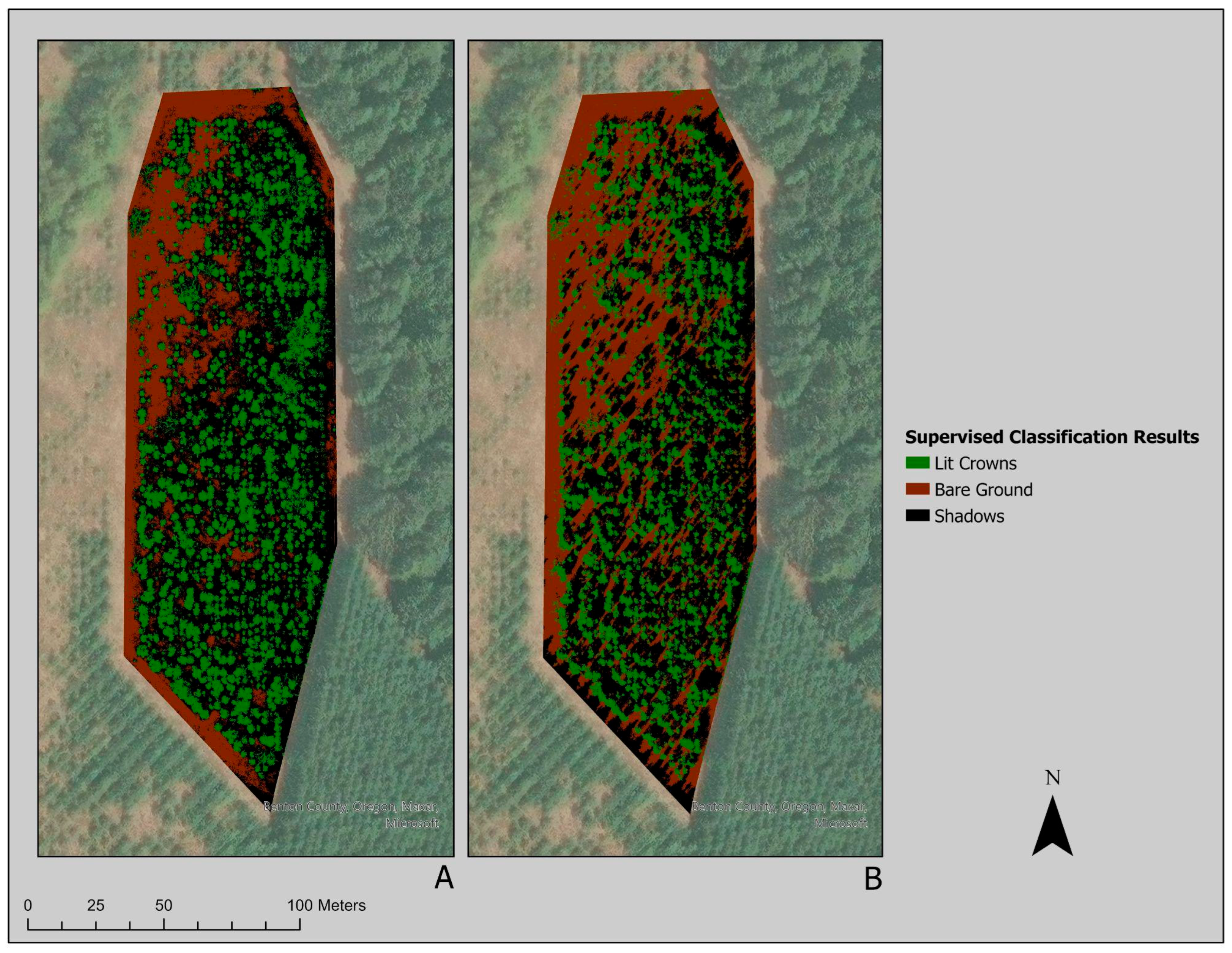
Using rasters of the entire Pacific Madrone orchard under both sunny and cloudy flight conditions (“the sunny and cloudy orthos”), we classified pixels in each raster as belonging to one of three classes (lit crowns, bare ground, or shadows), using ArGISPro’s Training Samples Manager as a part of its Imagery-Classification Tool workflow. We had approximately 160 samples per class. To create the sunny and cloudy classified output rasters, we used the Classify function as a part of the same workflow, selecting support vector machines as the supervised classification algorithm. From the rasters classified by SVM (“classified SVM rasters”), we extracted the lit crown pixels. We extracted the lit crown pixels from the classified SVM rasters by both selecting that class in the raster attribute table and using the Extract by Attribute Geoprocessing Tool, selecting “lit crowns” in the “class_name” column. We then converted those extracted output rasters into polygons with the Raster to Polygon Geoprocessing Tool, choosing not to simplify polygons, and identifying the relevant field by color (e.g., red). We next took the output polygons (“the tree crown polygons”), which conform to the crown volume of the entire Pacific Madrone orchard under both sunny and cloudy conditions, and imported them into RStudio (v4.4.2) for additional processing.
In RStudio, we also imported the sunny and cloudy orthos and converted the rasters into stacks with the following bands: “B”, “G”, “R”, “RE”, “NIR”, and “LWIR”. We examined the histograms for the B, G, R, and LWIR bands in both stacks to verify that each spectral band differed between flight conditions. We then used “band math” to create additional bands for each stack that corresponds to several vegetative indices (i.e., “TGI”, “GRVI”, “NDVI”, “NDRE”, “GNDVI”, “MSR”, “MSRE”, “GCI”, “RECI”). For simplicity, we will call these expanded stacks the sunny and cloud stacks. Using the terra::rast function in the terra package in R, we combined the sunny and cloudy stacks with the tree crown polygons. These combinations (“the sunny and cloudy crown statistics”) were then converted into data objects that allowed us to analyze and visualize the correlations between variables within each condition and between variables across conditions, using cor() and corrplot() in R. Below is a sample code, where M1 refers to the sunny crown statistics and M2 refers to the cloudy crown statistics:
  • M1 < -cor(crn_stats_su[,c(“B”, “G”, “R”, “RE”, “NIR”, “LWIR”, “TGI”, “GRVI”, “NDVI”, “NDRE”, “GNDVI”, “MSR”, “MSRE”, “GCI”, “RECI”)])
  • corrplot(M1, method = “number”)
  • M2 < -cor(crn_stats_cl[,c(“B”, “G”, “R”, “RE”, “NIR”, “LWIR”, “TGI”, “GRVI”, “NDVI”, “NDRE”, “GNDVI”, “MSR”, “MSRE”, “GCI”, “RECI”)])
  • corrplot(M2, method = “number”)
Although M1 and M2 have the same number of columns, corresponding to the spectral variables of interest, they have different lengths, due to the cloudy rasters featuring a greater number of observations. Even so, we visualized the correlation between the sunny crown statistics and cloudy crown statistics for the entire Pacific Madrone orchard using cor() and corrplot() in R:
  • b < -cor(M1, M2)
  • corrplot(b, addCoef.col = ‘green’, tl.cex = 1.2, tl.col = ‘black’, method = ‘color’)
Additionally, we calculated the R-squared and p values, all of which were significant at the <0.001 level.

2.6. Analysis of Survey Trees Using Spectral Variables of Interest

To analyze the surveyed trees using vegetative indices, we hand-digitized the 29 survey tree crowns in ArcGISPro (v3.5), using geolocation data from the 2019 survey of the Pacific Madrone plot, as well as sunny and cloudy orthos georeferenced to the 2019 ortho. This shapefile captured all 29 survey tree crowns in both the sunny and cloudy orthos. To ensure capturing as many useful pixels as possible, we used an irregular Polygon Tool to digitize the survey tree crowns. Once that shapefile was imported into RStudio, we combined it with a csv file containing the 2024 survey data (e.g., tree height, blight measurements, tree id, etc.). Using the terra::rast function in the terra package in R, we combined that with the sunny and cloudy stacks (for the entire Pacific Madrone orchard). We then extracted the spectral data from the sunny and cloudy stacks within the survey tree crown polygons, using the terra::extract function in R. After examining the histograms for NDVI, GRVI, and TGI indices in both data frames (“sunny data” and “cloudy data”) to verify that they differed, we used the sunny and cloudy data to compare each spectral band/index using paired t-tests for within-pair variation. The sample code is shown as follows:
  • t.test(cl_d$B, su_d$B, paired = TRUE)
  • t.test(cl_d$G, su_d$G, paired = TRUE)
  • t.test(cl_d$R, su_d$R, paired = TRUE)
With the addition of a “condition” column (0 for sunny, 1 for cloudy), we combined the two data frames and ran linear regressions on each spectral band/index for within- and between-pair variation. The sample code is shown as follows:
  • survB < -lm(survey_condition_test$B [1:29]~survey_condition_test$B [30:58], data = survey_condition_test)
  • summary(survB)

Blight Index Modeling of the Survey Tree Crowns Across Sunny and Cloudy Conditions

To identify which spectral variables best enable detection of blight under either the sunny or cloudy flight condition, we created a blight index out of the blight measurements in the 2024 survey data (see Ground Survey, above). Provided below is the first component of the blight index and the ultimate formula for creating that continuous variable, using the sunny data:
  • sunny_data$blight_0a[sunny_data$Blight_0 < 25] < −1
  • sunny_data$blight_0a[sunny_data$Blight_0 ≥ 25 & sunny_data$Blight_0 ≤ 50] < −2
  • sunny_data$blight_0a[sunny_data$Blight_0 > 50 & sunny_data$Blight_0 ≤ 75] < −3
  • sunny_data$blight_0a[sunny_data$Blight_0 > 75] < −4
  • sunny_data$blight_ind < −0 * sunny_data$blight_0a + 1 * sunny_data$blight_0_25a + 5 * sunny_data$blight_25_50a + 25 * sunny_data$blight_50a
Using both the sunny data (29 observations) and the cloudy data (29 observations) in a combined data frame (mentioned above in example code as “survey_condition_test”), we used the ranger package in R to identify variable importance for the Random Forest classification of the sunny or cloudy condition (0 or 1) and the Random Forest regression of blight index (whose values ranged from 31 to 106), employing out-of-bag (OOB) error estimation, which provides an internal measure of model validation without requiring a separate test set. We used all 58 observations and 1000 trees because the purpose was to inform feature selection for downstream linear modeling. Based on those variable importance rankings, we ran 5 multiple linear regressions using the lm() function in R to predict the blight index in the data frame consisting of both sunny and cloudy data. In Model 1, we predicted blight index with G, RE, Height, MSRE, NDRE, GNDVI, GCI, and RECI. In Model 2, we predicted blight index with B, R, Height, LWIR, NDRE, MSRE, and RECI. In Model 3, we predicted blight index with B, R, Height, NIR, LWIR, TGI, NDVI, GRVI, and MSR. In Model 4, we predicted blight index with R, B, Height, GCI, NIR, NDVI, MSR, and GNDVI. In Model 5, we predicted blight index with R, B, Height, GCI, NIR, MSR, and GNDVI. An example code is shown as follows:
  • model1 < -summary(lm(blight_ind~G + RE + Height + MSRE + NDRE + GNDVI + GCI + RECI, data = survey_condition_test))
  • model1
  • model2 < -summary(lm(blight_ind~B + R + Height + LWIR + NDRE + MSRE + RECI, data = survey_condition_test))
  • model2
  • model3 < -summary(lm(blight_ind~B + R + Height + NIR + LWIR + TGI + NDVI + GRVI + MSR, data = survey_condition_test))
  • model3
  • model4 < -summary(lm(blight_ind~R + B + Height + GCI + NIR + NDVI + MSR + GNDVI, data = survey_condition_test))
  • model4
  • model5 < -summary(lm(blight_ind~R + B + Height + GCI + NIR + MSR + GNDVI, data = survey_condition_test))
  • model5

3. Results

3.1. Results of Supervised Classification of Entire Pacific Madrone Plot Using Support Vector Machines

We generated a correlation matrix comparing all indices and bands for the sunny and cloudy crown volumes for the lit crowns only (Figure 2). The Pearson’s correlation coefficient showed the relationship between two variables on a scale of −1 to 1, with −1 being a perfect negative linear correlation, 1 being a perfect positive linear correlation, and 0 as having no correlation. The sunny NDRE values and the cloudy NDRE values were correlated with a Pearson’s correlation coefficient of 0.96. A close and similar correlation of 0.97 was found for NDVI. Overall, indices (RECI, NDRE, MSRE, GNDVI, GCI, NDVI, MSR, GRVI, TGI) had high positive correlation, ranging from 0.86 (TGI) to 0.97 (GCI), with the exception of GRVI (0.57). The correlations for bands (R, G, B, NIR, RE, LWIR) were also high but slightly lower than the indices, ranging from 0.80 (NIR) to 0.98 (R).

3.2. Supervised Classification Accuracy Assessment

A supervised classification accuracy assessment was completed using ArcGIS Pro to determine how accurately the computer could distinguish between lit crowns, bare ground, and shadows in the sunny ortho imagery. This assessment included creating 33 random crown points, 26 random ground points, and 40 random shadow points within our designated area but not lying within the predetermined polygons we used to train the computer model. These points were then each assessed by hand and assigned a value, 1–3, depending on what category the point represented, where 1 = lit crowns, 2 = bare ground, and 3 = shadows. Following categorization, we created a confusion matrix to determine the computer model’s accuracy on a random selection of points which fell into each of the three desired categories (Table 2). The SVM supervised classification performance, based on the confusion matrix generated from the 100 datapoints, is as follows: kappa = 0.87 (95% CI: 0.84, 0.96), balanced accuracy = 0.93, and true positive rate (lit crowns) = 97%.

3.3. Results of Linear Regression of 29 Survey Tree Crowns

We conducted linear regression of each spectral band/index for the 29 survey tree crowns across sunny and cloudy conditions. Table 3 shows the adjusted R-squared and p-values for linear regressions of the cloudy and sunny data for the 29 survey tree crowns, with cloudy as the independent variable (x) and sunny as the dependent variable (y).
The adjusted R-squared values show how much of the variability in sunny band or index values can be explained by the corresponding cloudy band or index, with the adjusted R-squared ranging from 0.23 (LWIR) to 0.95 (NDVI). The highest adjusted R-squared values were for NDVI (adjusted R2 =0.95), MSRE (adjusted R2 = 0.95), and RECI (adjusted R2 = 0.95), showing that, for those specific indices, the images on cloudy days explained over 94% of the variability of their corresponding index values on sunny days. The lowest adjusted R-squared value was for LWIR, with the cloudy image only explaining 23.49% of the variability in the sunny image.

3.4. Results of Paired T-Tests of 29 Survey Tree Crowns

We conducted paired t-tests on the 29 survey tree crowns across the sunny and cloudy conditions (Table 4). The mean difference from a paired t-test is identified whether there is a statistically significant difference between the two conditions (sunny, cloudy) in identical crowns. The greatest mean difference that we identified was −9.903 for MSR. The smallest mean difference we identified was −0.012 for blue. All mean differences were statistically significant at the <0.01 level.

3.5. Results of Blight Index Modeling Using Multiple Linear Regression

We used multiple linear regression to model blight in a dataset consisting of 58 observations (29 cloudy survey crowns and 29 sunny survey crowns). The results of our blight index modeling using multiple linear regression revealed that our blight index, across sunny and cloudy conditions, was a function of the following independent variables, all of which were statistically significant at the <0.05 level: red, blue, height, GCI, NIR, MSR, and GNDVI. Model 5 was our best performing model at predicting blight index within the survey tree crowns across both sunny and cloudy conditions. The adjusted R-squared for the overall model was 0.25, indicating that it explained 25% of the variance in the blight index across sunny and cloudy conditions. The p-value for the overall model was significant at the <0.01 level (p = 0.0025).
Given that our final blight prediction model (model 5) had a sample size of 58 and 7 variables, we took the 10 variables from the best performing multiple linear regression models (models 3 to 5) other than LWIR, whose inconsistency/variation can already be explained by intraday cloud drift, and performed AIC model selection with the Multi-Model Inference package in R. The best performing model, in terms of AIC, consisted of the blue band, the red band, and tree height (AIC = 497.9, R2 = 0.19). The second best performing model, in terms of AIC, consisted of GVRI, the red band, and tree height (AIC = 498.7, R2 = 0.18). The third best performing model, in terms of AIC, consisted of tree height (AIC = 498.8, R2 = 0.14). The fourth best performing model, in terms of AIC, consisted of the red band, the blue band, tree height, GCI, NIR, MSR, and GDNDVI (AIC = 499.2, R2 = 0.25). The fourth best performing model, in terms of AIC, is our final blight prediction model (model 5).

4. Discussion

4.1. Contribution to Literature

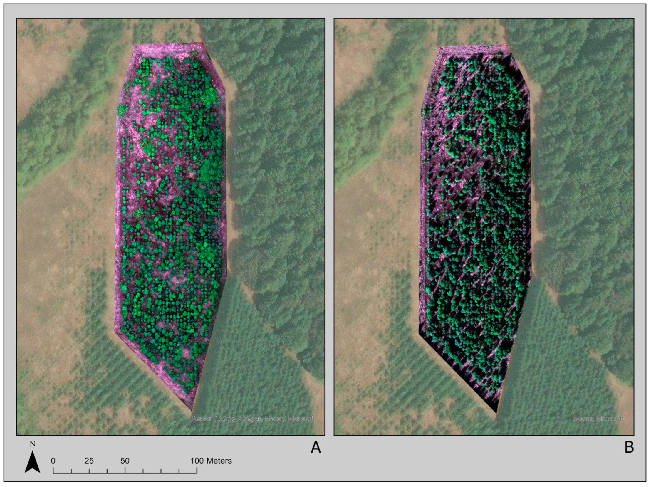
Our study improved upon the prior literature and research studies examining differences between spectral indices across sunny and cloudy conditions (see Figure 3). Our contribution mainly consists of the following: (a) confirming index-dependent differences with multispectral UAS sensors (which can be less sensitive to differences in skylight conditions than hyperspectral sensors), (b) expanding the range of vegetation indexes under evaluation, (c) conducting paired t-tests of within-canopy data, allowing for an inference of a role for canopy architecture, and (d) using SVM for tree crown classification, including the classification and/or elimination of shadows (see Figure 4).
First, we established that multispectral UAS surveys have sufficient sensitivity. Arroyo-Mora et al., using a full-range pushbroom hyperspectral UAS sensor (400–2500 nm) under variable cloud cover and skylight conditions, found statistically significant index-dependent differences across cloudy and sunny conditions for the following spectral indices: NDVI, CRI, ARI2, CAI, NDLI, and NDWI [10]. Similarly, using a multispectral UAS sensor, we found statistically significant band- or index-dependent differences across cloudy and sunny conditions for the following spectral indices/variables: B, G, R, RE, NIR, LWIR, TGI, GRVI, NDVI, NDRE, GNDVI, MSR, MSRE, GCI, and RECI. Additionally, our paired t-tests identified within canopy band- or index-dependent differences for the same spectral bands/indices, suggesting a role for canopy architecture (see Table 4, above).
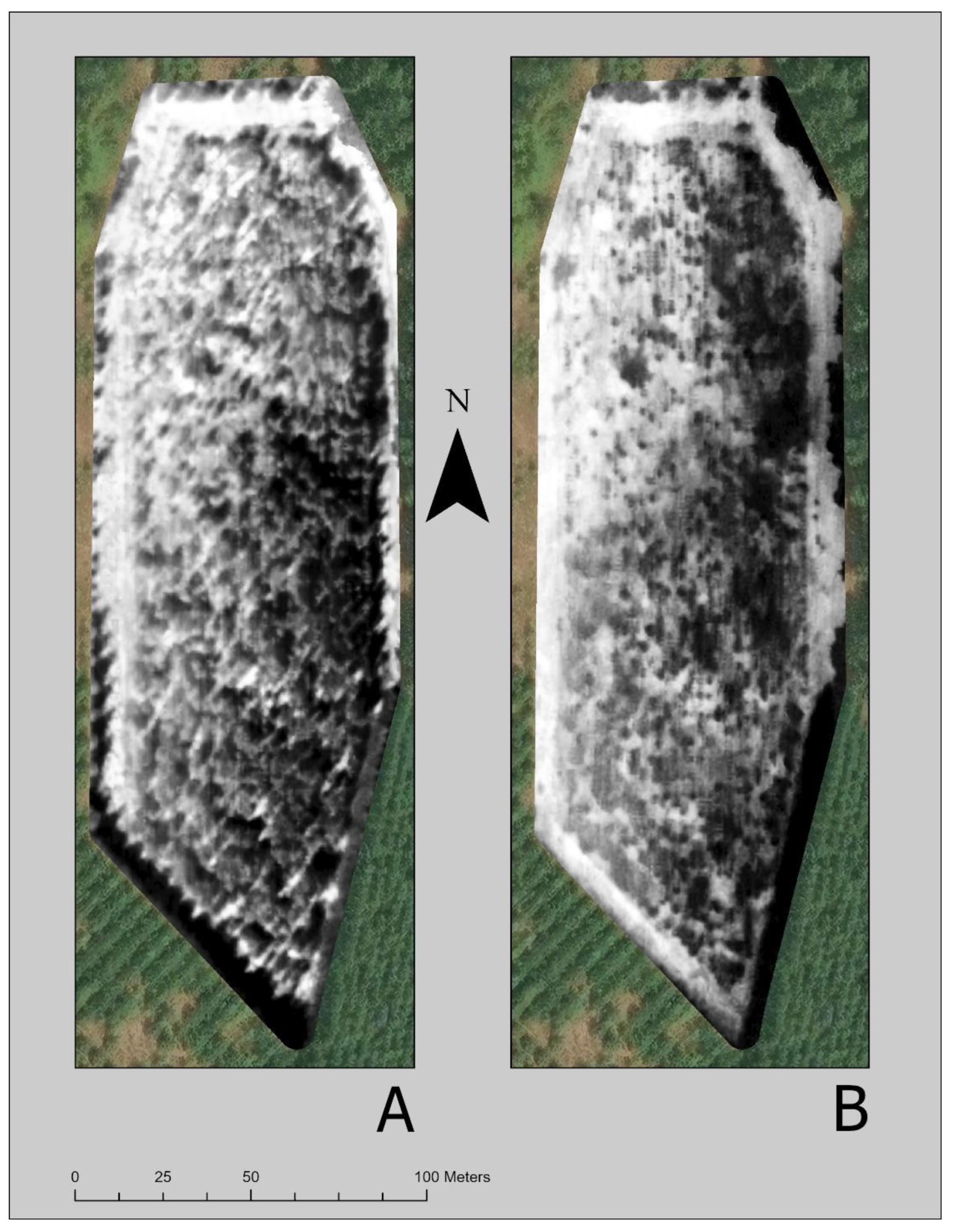
Moreover, we identified at least one spectral difference caused by cloud cover. De Souza et al. compared active sensors (a Crop Circle ACS-470 (Holland Scientific, Inc., Lincoln, NE, USA) and a Greenseeker RT100 (NTech Industries, Inc., Ukiah, CA, USA)), passive sensors (a hyperspectral bidirectional passive spectrometer and a HandySpec Field sensor (tec5 AG, Steinbach, Germany)), and UAS imagery captured with a Parrot Sequoia multispectral sensor (Parrot SA, Paris, France) to identify differences due to time of day and cloud cover in the multiple spectral indices [7]. The spectral indices included NDVI, GNDVI, NIR/Red, NIR/Green, NIR/Red edge, Red edge/Red, Water Index WI (R900/R970), and Red Edge Inflection Point (REIP). Using linear regression, they found that indexes mainly self-agreed across sunny and cloudy conditions, but there were statistically significant differences across cloudy and sunny conditions, with the most stable differences in NIR/Red edge ratio, Water Index WI (R900/R970), and REIP. With respect to NDVI, De Souza et al. inferred that the variability in NDVI was due to reduced solar radiation under cloud cover [7]. Similarly, we used linear regression to find significant agreement across the following spectral indices/variables under sunny and cloudy conditions: B, G, R, RE, NIR, LWIR, TGI, GRVI, NDVI, NDRE, GNDVI, MSR, MSRE, GCI, and RECI (see Table 3, above). With respect to LWIR, however, we found the smallest amount of self-agreement across sunny and cloudy conditions, consistent with the impact of cloud cover blocking sunlight and trapping longwave radiation (Figure 5) [30]. Attributing the low R2 value to cloud drift effects—specifically the transient trapping and release of LWIR radiation as clouds move across the scene diurnally—is consistent with our paired t-test results (see Table 4, above), which show a positive mean difference for the red band (0.016) and negative mean differences for the blue, near infrared, and longwave radiation bands (−0.012, −0.211, and −4.183, respectively).
Importantly, while most UAS surveys for disease monitoring purposes use deep learning (i.e., convolutional neural networks or CNNs) and Random Forest algorithms for the classification of tree crowns [4], we contributed to the SVM literature on tree crown classification, e.g., [31], demonstrating that our methods provide a high level of accuracy (see Section 3.2, above) and enable reliable within-crown statistical analysis.
In addition to improving upon the prior literature and research studies on index-dependent spectral differences between sunny and cloudy conditions, we also confirmed findings from prior studies relating both to forest disease monitoring with UAS [5,6] and spectral imaging from UAS under variable illumination [8]. Wing and Barker found that several spectral vegetation indices strongly correlated under cloudy flight conditions in October 2019 (GVRI, MSR, NDVI, and TGI), with GVRI showing the strongest correlation with blight presence [6]. Furthermore, they found a statistically significant relationship between the D8 flow accumulation model and blight presence [6]. Here, we found that the Red, Blue, GCI, NIR, MSR, and GNDVI spectral variables best explained the presence of blight within Pacific Madrone tree crowns under both cloudy and sunny conditions. As a part of the same multiple linear regression model, which was informed by our use of Random Forest for feature selection, we found that tree height has a statistically significant inverse relationship with blight presence. While the relationships between the specific spectral vegetation indices in Wing and Barker and our study are different, what the findings in both have in common is cloudy conditions improve the performance of certain spectral indices due to atmospheric scattering caused by cloud cover [32]. This is directly in line with Barker et al. who found that, in predicting the presence of blight in Pacific Madrone tree crowns using Random Forest classification, “[s]pectral predictors including mean reflectance in red and blue bands had relatively high importance to model accuracy” [5]. Notably, our AIC model selection confirmed this prior research. The best performing model, in terms of AIC, is consistent with Barker, et al. [5]; the second best performing model, in terms of AIC, is consistent with Wing and Barker [6]. Lastly, we were able to use multispectral UAS to achieve results consistent with the prior literature without the need for Tucker tensor decomposition [33] and/or capturing signal-to-noise ratio data [10], indicating that, like Hakala et al., “high accuracy UAV remote sensing, with stereoscopic and spectrometric capabilities, is possible also in diverse conditions,” making such methods “suitable for many environmental measurement and monitoring applications” [8].

4.2. Flight Timing

Our initial UAS flight was conducted during cloudy weather conditions on 18 October 2024. We repeated the flight under more favorable, sunny conditions on 24 October 2024. However, the flights were not conducted at the same time of day. The cloudy flight occurred at approximately 1:00 p.m. PST, closer to solar noon, while the sunny flight occurred later at 3:00 p.m. PST. Notably, in October, solar noon in Oregon occurs near 1:00 p.m., and sunset follows around 6:30 p.m. One would expect this shift in the sun’s angle over the short afternoon period to alter the lighting conditions for the two different flight timings, influencing shadowing, contrast, and canopy reflectance in the imagery. We would also expect that the strong, positive correlations we observed in spectral bands and indices between light conditions would have been strengthened had the second flight occurred closer to solar noon.

4.3. Connection to Madrone Health

Our findings demonstrate the effects cloudy weather may have on orthomosaics created for applying machine learning tree segmentation algorithms to Pacific Madrone tree stands. Understanding how weather can impact band accuracy (or the accuracy of vegetation indices under conditions of decreased red and increased blue, near infrared, and longwave infrared electromagnetic radiation) has real world consequences for combating Pacific Madrone tree blight. The leaf spots we saw in the field are likely a result of fungal pathogens, which are transmittable both airborne and through water splashing from one affected leaf to another [2]. To limit the spread of these pathogens to unaffected Madrone stands, efficiently understanding the scale of the issue is necessary to give resource managers the ability to perform countermeasures. These measures can take place in the form of pruning affected branches and racking/removing affected leaves prior to a rainstorm [2]. Since the fungal pathogens transmit primarily through water during rainstorms, being able to obtain fast and accurate data is necessary in a Mediterranean-type environment such as the Willamette Valley. Rapid and accurate data acquisition can allow resource managers the ability to both analyze the data and act on it in between rainstorms, depending on the intermission between storms, which will greatly improve Madrone state resistivity. Through the combination of modern UAS, onboard sensors, and previous Madrone conservation knowledge, helping preserve the Pacific Northwest native Madrone tree will be more time and cost efficient.

5. Conclusions

5.1. Key Findings

First, we found high levels of agreement across cloudy and sunny conditions for several commonly used vegetative indices (e.g., NDVI [adjusted R2 = 0.95], MSRE [adjusted R2 = 0.95], RECI [adjusted R2 = 0.95], GCI [adjusted R2 = 0.92], MSR [adjusted R2 = 0.92], and GNDVI [adjusted R2 = 0.92]) (See Table 3). This suggests flying under conditions in deviation from traditional guidelines may be acceptable practice, expanding the range of potential flight schedules for UAS disease surveys.
Second, cloud cover may improve blight detection. Contrary to the intuition that cloud cover may impair remote sensing work by changing shadows, contrast, and canopy reflectance, we found that diffuse skylight conditions under cloud cover make certain wavelengths more available (e.g., blue and near infrared), make certain wavelengths less available (e.g., red) (Table 4), and improve the performance of certain vegetation indexes (GCI, MSR, and GNDVI). Our relatively most explanatory and least noisy multiple linear regression model (p = 0.0025, AIC = 497.9) indicated that the most robust predictors of foliar blight in Pacific Madrone crowns across sunny and cloudy conditions were the red, blue, and near infrared bands, the GCI, MSR, and GNDVI vegetative indexes, and tree height.
Third, with respect to tree structure, all our multiple linear regression models showed that tree height and foliar blight presence have a statistically significant inverse relationship (p < 0.005). Additionally, we were able to show that band- and index-dependent spectral differences are present within canopies at the <0.01 level (Table 4), suggesting that canopy architecture—not just the presence of chlorophyll—plays a role.
Lastly, our tree crown delineation method, using SVM to perform a supervised classification of tree crowns, bare ground, and shadows, yielded a kappa of 0.865, a balanced accuracy of 92.5%, and a true positive rate of 97% (Table 2).

5.2. Future Directions

Given our key findings, future directions for this field of research are at least four-fold. First, the type of cloud cover may impact the variability of vegetative index performance on detecting foliar blight. We did not conduct a systematic analysis of different cloud types (e.g., cumulus, altocumulus, and cirrus clouds) on ambient electromagnetic radiation and/or solar irradiance. Second, given the association of foliar blight with Madrone decline, an inverse relationship between tree height and foliar blight presence could be an indication of resilience that may be associated with underlying site hydrology. It is an open question whether our findings apply to non-orchards, where Pacific Madrones may be in competition with other tree species. Third, the multispectral sensor we used for our UAS flights does not have a shortwave infrared (SWIR) band. SWIR has proven to be useful in detecting foliar diseases in laboratory settings and glasshouse conditions [34,35]. Given the usefulness of SWIR in detecting vegetation liquid [36], future research on UAS blight detection under variable illumination could incorporate multispectral UAS sensors that include a SWIR band and compare the performance of NDWI and NDII [37] to other vegetation indexes in addition to the red and blue bands. Fourth, although we had success with SVM, filling a gap in the literature, where CNNs and Random Forest are typically used for crown classification, a comparative study of SVM versus other ML algorithms for this classification task could be a future direction.
Previous publications from the AIS lab [5,6] and others [38] demonstrate the transformative potential of UAS, onboard sensors such as multispectral cameras, and machine learning algorithms in expanding the scope and depth of ecological and environmental investigations. These rapidly developing technologies enable us to gather actionable, high-resolution data that reveal intricate patterns and processes in the natural world. In an era of variable climate and shrinking budgets, UAS remote sensing, enhanced by the power of machine learning, offers a cost-effective and efficient method to actively survey and monitor and preserve critical resources and places of interest.

Author Contributions

Conceptualization, M.C.W. and M.G.W.; methodology, M.C.W.; software, M.C.W.; validation, M.C.W. and M.G.W.; formal analysis, M.C.W., J.H.W., S.G., A.M.A., D.C.H., A.H.M. and M.G.W.; investigation, M.C.W., J.H.W., S.G., A.M.A., D.C.H., A.H.M. and M.G.W.; resources, M.C.W., J.H.W., S.G., A.M.A., D.C.H., A.H.M. and M.G.W.; data curation, M.C.W., J.H.W., S.G., A.M.A., D.C.H., A.H.M. and M.G.W.; writing—original draft preparation, M.C.W., J.H.W., S.G., A.M.A., D.C.H., A.H.M. and M.G.W.; writing—review and editing, M.C.W., J.H.W., S.G., A.M.A., D.C.H., A.H.M. and M.G.W.; visualization, M.C.W. and J.H.W.; supervision, M.G.W.; project administration, M.G.W. All authors have read and agreed to the published version of the manuscript.

Funding

This research received no external funding.

Data Availability Statement

The raw data supporting the conclusions of this article will be made available by the authors upon request.

Acknowledgments

We appreciate being able to measure and image the Pacific Madrone orchard with access provided by Starker Forests, Inc, Corvallis, OR, USA. We also thank Matt Barker for creating a confusion matrix for our image classification results.

Conflicts of Interest

The authors declare no conflicts of interest. The funders had no role in the design of the study; in the collection, analyses, or interpretation of data; in the writing of the manuscript; or in the decision to publish the results.

References

  1. Immel, D.L. Plant Guide: Pacific Madrone; USDA, NRCS: Washington, DC, USA, 2006. Available online: https://plants.usda.gov/DocumentLibrary/plantguide/pdf/cs_arme.pdf (accessed on 11 November 2024).
  2. Bennett, M.; Shaw, D.C. Diseases and Insect Pests of Pacific Madrone; Oregon State University, Extension Service: Corvallis, OR, USA, 2008. [Google Scholar]
  3. Elliott, M. The Decline of Pacific Madrone (Arbutus menziesii Pursh) in Urban and Natural Environments: Its Causes and Management. Ph.D. Thesis, University of Washington, Seattle, WA, USA, 1999. [Google Scholar]
  4. Duarte, A.; Borralho, N.; Cabral, P.; Caetano, M. Recent advances in forest insect pests and diseases monitoring using UAV-based data: A systematic review. Forests 2022, 13, 911. [Google Scholar] [CrossRef]
  5. Barker, M.I.; Burnett, J.D.; Haddad, T.; Hirsch, W.; Kang, D.K.; Wing, M.G. Multi-temporal Pacific madrone leaf blight assessment with unoccupied aircraft systems. Ann. For. Res. 2023, 66, 171–181. [Google Scholar] [CrossRef]
  6. Wing, M.G.; Barker, M. Applying unoccupied aircraft system multispectral remote sensing to examine blight in a Pacific madrone orchard. Int. J. For. Hortic. 2024, 10, 20–30. [Google Scholar] [CrossRef]
  7. de Souza, R.; Buchhart, C.; Heil, K.; Plass, J.; Padilla, F.M.; Schmidhalter, U. Effect of time of day and sky conditions on different vegetation indices calculated from active and passive sensors and images taken from UAV. Remote Sens. 2021, 13, 1691. [Google Scholar] [CrossRef]
  8. Hakala, T.; Honkavaara, E.; Saari, H.; Mäkynen, J.; Kaivosoja, J.; Pesonen, L.; Pölönen, I. Spectral imaging from UAVs under varying illumination conditions. Int. Arch. Photogramm. Remote Sens. Spat. Inf. Sci. 2013, 40, 189–194. [Google Scholar] [CrossRef]
  9. Slade, G.; Anderson, K.; Graham, H.A.; Cunliffe, A.M. Repeated drone photogrammetry surveys demonstrate that reconstructed canopy heights are sensitive to wind speed but relatively insensitive to illumination conditions. Int. J. Remote Sens. 2025, 46, 24–41. [Google Scholar] [CrossRef]
  10. Arroyo-Mora, J.P.; Kalacska, M.; Løke, T.; Schläpfer, D.; Coops, N.C.; Lucanus, O.; Leblanc, G. Assessing the impact of illumination on UAV pushbroom hyperspectral imagery collected under various cloud cover conditions. Remote Sens. Environ. 2021, 258, 112396. [Google Scholar] [CrossRef]
  11. Guerra-Hernández, J.; González-Ferreiro, E.; Monleón, V.J.; Faias, S.P.; Tomé, M.; Díaz-Varela, R.A. Use of multi-temporal UAV-derived imagery for estimating individual tree growth in Pinus pinea stands. Forests 2017, 8, 300. [Google Scholar] [CrossRef]
  12. Gu, J.; Grybas, H.; Congalton, R.G. A comparison of forest tree crown delineation from unmanned aerial imagery using canopy height models vs. spectral lightness. Forests 2020, 11, 605. [Google Scholar] [CrossRef]
  13. Gu, J.; Grybas, H.; Congalton, R.G. Individual tree crown delineation from UAS imagery based on region growing and growth space considerations. Remote Sens. 2020, 12, 2363. [Google Scholar] [CrossRef]
  14. Guimarães, N.; Pádua, L.; Marques, P.; Silva, N.; Peres, E.; Sousa, J.J. Forestry remote sensing from unmanned aerial vehicles: A review focusing on the data, processing and potentialities. Remote Sens. 2020, 12, 1046. [Google Scholar] [CrossRef]
  15. PRISM Climate Group, Oregon State University. Available online: https://prism.oregonstate.edu (accessed on 5 December 2024).
  16. DeWald, L.E.; Elliott, M.; Sniezko, R.A.; Chastagner, G.A. Geographic and local variation in Pacific madrone (Arbutus menziesii) leaf blight. In Proceedings of the 6th International Workshop on the Genetics of Tree-Parasite Interactions: Tree Resistance to Insects and Diseases: Putting Promise into Practice, Mt. Sterling, OH, USA, 5–10 August 2018. [Google Scholar]
  17. Nesbit, P.R.; Hugenholtz, C.H. Enhancing UAV–SFM 3D model accuracy in high-relief landscapes by incorporating oblique images. Remote Sens. 2019, 11, 239. [Google Scholar] [CrossRef]
  18. Hostens, D.S.; Dogwiler, T.; Hess, J.W.; Pavlowsky, R.T.; Bendix, J.; Martin, D.T. Assessing the role of sUAS mission design in the accuracy of digital surface models derived from structure-from-motion photogrammetry. In sUAS Applications in Geography; Springer: Cham, Switzerland, 2022; pp. 123–156. [Google Scholar]
  19. Agisoft. Agisoft Metashape User Manual; Agisoft: St. Petersburg, Russia, 2024; Available online: https://www.agisoft.com/downloads/user-manuals/ (accessed on 11 November 2024).
  20. MicaSense, Inc. What is the Center Wavelength and Bandwidth of Each Filter for MicaSense Sensors? MicaSense, Inc.: Seattle, WA, USA, 2024; Available online: https://support.micasense.com/hc/en-us/articles/214878778-What-is-the-center-wavelength-and-bandwidth-of-each-filter-for-MicaSense-sensors (accessed on 27 August 2025).
  21. Hunt, E.R., Jr.; Daughtry, C.S.; Eitel, J.U.; Long, D.S. Remote sensing leaf chlorophyll content using a visible band index. Agronomy 2011, 103, 1090–1099. [Google Scholar] [CrossRef]
  22. Hunt, E.R., Jr.; Doraiswamy, P.C.; McMurtrey, J.E.; Daughtry, C.S.; Perry, E.M.; Akhmedov, B. A visible band index for remote sensing leaf chlorophyll content at the canopy scale. Int. J. Appl. Earth Obs. Geoinf. 2013, 21, 103–112. [Google Scholar] [CrossRef]
  23. Tucker, C.J. Red and photographic infrared linear combinations for monitoring vegetation. Remote Sens. Environ. 1979, 8, 127–150. [Google Scholar] [CrossRef]
  24. Rouse, J.W., Jr.; Haas, R.H.; Deering, D.W.; Schell, J.A.; Harlan, J.C. Monitoring the Vernal Advancement and Retrogradation (Green Wave Effect) of Natural Vegetation; Final Report, Type III for the Period September 1972–November 1974; Texas A&M University: Remote Sensing Center: College Station, TX, USA, 1974. [Google Scholar]
  25. Barnes, E.M.; Clarke, T.R.; Richards, S.E.; Colaizzi, P.D.; Haberland, J.U.; Kostrzewski, M.; Waller, P.; Choi, C.; Riley, E.; Thompson, T.; et al. Coincident detection of crop water stress, nitrogen status and canopy density using ground-based multispectral data. In Proceedings of the Fifth International Conference on Precision Agriculture, Bloomington, MN, USA, 16 July 2000; Volume 1619. No. 6. [Google Scholar]
  26. Gitelson, A.A.; Kaufman, Y.J.; Merzlyak, M.N. Use of a green channel in remote sensing of global vegetation from EOS-MODIS. Remote Sens. Environ. 1996, 58, 289–298. [Google Scholar] [CrossRef]
  27. Chen, J.M. Evaluation of vegetation indices and a modified simple ratio for boreal applications. Can. J. Remote Sens. 1996, 22, 229–242. [Google Scholar] [CrossRef]
  28. Cao, Q.; Miao, Y.; Wang, H.; Huang, S.; Cheng, S.; Khosla, R.; Jiang, R. Non-destructive estimation of rice plant nitrogen status with Crop Circle multispectral active canopy sensor. Field Crops Res. 2013, 154, 133–144. [Google Scholar] [CrossRef]
  29. Gitelson, A.A.; Viña, A.; Ciganda, V.; Rundquist, D.C.; Arkebauer, T.J. Remote estimation of canopy chlorophyll content in crops. Geophys. Res. Lett. 2005, 32, L08403. [Google Scholar] [CrossRef]
  30. Luo, H.; Quaas, J.; Han, Y. Diurnally asymmetric cloud cover trends amplify greenhouse warming. Sci. Adv. 2024, 10, eado5179. [Google Scholar] [CrossRef]
  31. Xiao, D.; Pan, Y.; Feng, J.; Yin, J.; Liu, Y.; He, L. Remote sensing detection algorithm for apple fire blight based on UAV multispectral image. Comput. Electron. Agric. 2022, 199, 107137. [Google Scholar] [CrossRef]
  32. Mol, W.; Heusinkveld, B.; Mangan, M.R.; Hartogensis, O.; Veerman, M.; van Heerwaarden, C. Observed patterns of surface solar irradiance under cloudy and clear-sky conditions. Q. J. R. Meteorol. Soc. 2024, 150, 2338–2363. [Google Scholar] [CrossRef]
  33. Wang, S.; Baum, A.; Zarco-Tejada, P.J.; Dam-Hansen, C.; Thorseth, A.; Bauer-Gottwein, P.; Bandini, F.; Garcia, M. Unmanned Aerial System multispectral mapping for low and variable solar irradiance conditions: Potential of tensor decomposition. ISPRS J. Photogramm. Remote Sens. 2019, 155, 58–71. [Google Scholar] [CrossRef]
  34. Ahlawat, V.; Jhorar, O.; Kumar, L.; Backhouse, D. Using hyperspectral remote sensing as a tool for early detection of leaf rust in blueberries. In Proceedings of the International Symposium on Remote Sensing of Environment—The GEOSS Era: Towards Operational Environmental Monitoring, Sydney, Australia, 10–15 April 2011. [Google Scholar]
  35. Gorretta, N.; Nouri, M.; Herrero, A.; Gowen, A.; Roger, J.M. Early detection of the fungal disease “apple scab” using SWIR hyperspectral imaging. In Proceedings of the 10th Workshop on Hyperspectral Imaging and Signal Processing: Evolution in Remote Sensing (WHISPERS), Amsterdam, The Netherlands, 24–26 September 2019; pp. 1–4. [Google Scholar]
  36. Stark, B.; McGee, M.; Chen, Y. Short wave infrared (SWIR) imaging systems using small Unmanned Aerial Systems (sUAS). In Proceedings of the 2015 International Conference on Unmanned Aircraft Systems (ICUAS), Denver, CO, USA, 9–12 June 2015; pp. 495–501. [Google Scholar]
  37. Ji, L.; Zhang, L.; Wylie, B.K.; Rover, J. On the terminology of the spectral vegetation index (NIR− SWIR)/(NIR+ SWIR). Int. J. Remote Sens. 2011, 32, 6901–6909. [Google Scholar] [CrossRef]
  38. Marques, P.; Pádua, L.; Adão, T.; Hruška, J.; Peres, E.; Sousa, A.; Sousa, J.J. UAV-based automatic detection and monitoring of chestnut trees. Remote Sens. 2019, 11, 855. [Google Scholar] [CrossRef]
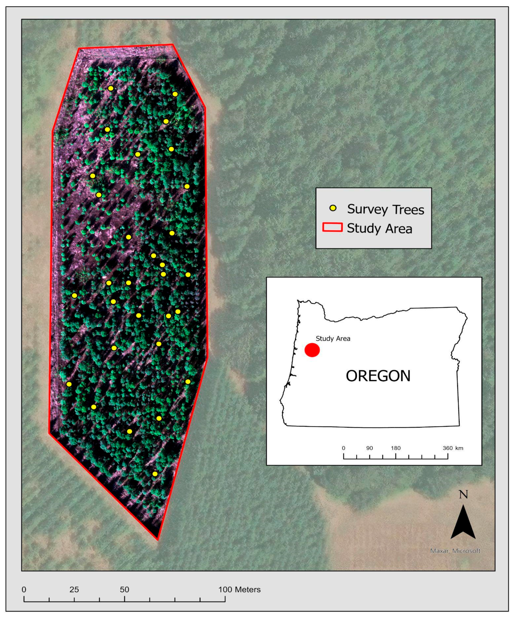
Figure 1. Study area location. Credit: Esri, Benton County, Oregon, Maxar, Microsoft.
Remotesensing 17 03141 g001
Figure 2. Pearson correlation values (r) for Pacific Madrone crowns imaged in sunny (x-axis) and overcast conditions (y-axis). Table 1 contains the abbreviation key.
Remotesensing 17 03141 g002
Figure 3. Orthographic images for (A) cloudy conditions and (B) sunny conditions. Credit: Esri, Benton County, Oregon, Maxar, Microsoft.
Remotesensing 17 03141 g003
Figure 4. Supervised classification results for (A) cloudy conditions and (B) sunny conditions. Credit: Esri, Benton County, Oregon, Maxar, Microsoft.
Remotesensing 17 03141 g004
Figure 5. A side-by-side comparison of the thermal (LWIR) band from our multispectral UAS sensor. The sunny flight is on the left (A); the cloudy flight is on the right (B). The cloudy LWIR explains only ~23% of the variability in the sunny LWIR.
Remotesensing 17 03141 g005
Table 1. Vegetation indices constructed from individual bands 1–6. Formula describes how vegetation indices are derived, and reference denotes the source of the VI.
Band Name or Vegetation IndexFormula *Reference
  • Blue (B)
475 ± 32 nm[20]
2.
Green (G)
560 ± 27 nm[20]
3.
Red (R)
668 ± 14 nm[20]
4.
Red edge (RE)
717 ± 12 nm [20]
5.
Near infrared (NIR)
842 ± 57 nm [20]
6.
Longwave infrared (LWIR)
~11 µm (11,000 nm), bandwidth ~6 µm [20]
7.
Triangular Greenness Index (TGI)
–0.5 × [190 × (R − G) − 120 × (R − B)][21,22]
8.
Green red Vegetation Index (GRVI)
NIR/G[23]
9.
Normalized Difference Vegetation Index (NDVI)
(NIR − R)/(NIR + R)[24]
10.
Normalized Difference Red Edge (NDRE)
(NIR − RE)/(NIR + RE)[25]
11.
Green Normalized Difference Vegetation Index (GNDVI)
(NIR − G)/(NIR + G)[26]
12.
Modified Simple Ratio Index (MSR)
(NIR/R − 1)/(√(NIR/R) + 1)[27]
13.
Modified Simple Ratio Index Red Edge (MSRE)
(NIR/RE − 1)/(√(NIR/RE) + 1)[28]
14.
Green Chlorophyll Index (GCI)
(NIR/G) − 1[29]
15.
Red Edge Chlorophyll Index (RECI)
(NIR/RE) − 1[29]
* Wavelength associated with band and R is a reflectance of the corresponding band: blue (B), green (G), red (R), red edge (RE), near infrared (NIR).
Table 2. Confusion matrix: Aggregated cell counts. Cells on the diagonal axis indicate random points correctly identified by the SVM classification.
PredictionReference
Class123
13202
21266
30033
Table 3. Adjusted R2 and p-values for the linear regression of all bands/indexes under cloudy (x) and sunny (y) conditions. The p-values for all relationships were highly and positively significant (p < 0.005), suggesting that the correlation between cloudy and sunny data was high for all bands and indices other than LWIR. LWIR had a statistically significant low positive correlation. Table 1 contains the abbreviation key.
Band/IndexAdjusted R2p-ValueRSE
B0.66<0.0050.00
G0.82<0.0050.00
R0.62<0.0050.00
RE0.80<0.0050.03
NIR0.84<0.0050.05
LWIR0.23<0.0051.67
TGI0.87<0.0050.54
GRVI0.91<0.0050.00
NDVI0.95<0.0050.00
NDRE0.95<0.0050.01
GNDVI0.92<0.0050.00
MSR0.92<0.0050.01
MSRE0.95<0.0050.03
GCI0.92<0.0050.48
RECI0.95<0.0050.07
Table 4. Mean differences and p-values for paired t-tests of survey tree crowns under cloudy and sunny conditions. The mean differences were small across most cloudy and sunny pairs of crowns; the largest differences were found within the MSR, LWIR, and TGI bands/indices. Table 1 contains the abbreviation key.
Band/IndexMean Differencep-Value
B−0.012<0.005
G−0.024<0.005
R0.016<0.005
RE−0.094<0.005
NIR−0.211<0.005
LWIR−4.183<0.005
TGI−2.394<0.005
GRVI−0.505<0.005
NDVI−0.108<0.005
NDRE−0.008<0.005
GNDVI−0.018<0.005
MSR−9.903<0.005
MSRE−0.023<0.005
GCI−0.823<0.005
RECI−0.056<0.005
Disclaimer/Publisher’s Note: The statements, opinions and data contained in all publications are solely those of the individual author(s) and contributor(s) and not of MDPI and/or the editor(s). MDPI and/or the editor(s) disclaim responsibility for any injury to people or property resulting from any ideas, methods, instructions or products referred to in the content.