GEO SAR Refocusing Algorithm of Ship Targets with Complex Motion via CFSFD-Based ISAR Technique

Highlights

What are the main findings?

• The Geosynchronous synthetic aperture radar (GEO SAR) received signal from ship targets with complex motion is derived and modeled as a multicomponent 2-D joint sine-series-polynomial phase signal (2-D JSPS). In addition, a joint envelope-phase estimation named complex fast-time slow-time frequency distribution (CFSFD) is proposed to achieve instantaneous frequency estimation for such a signal.
• A GEO SAR refocusing algorithm for ship targets with complex motion is proposed, which is a hybrid SAR/ISAR refocusing algorithm. In this algorithm, CFSFD-based range-migration-correction-free inverse SAR (RMC-free ISAR) technique is used to replace the existing RMC, followed by the time–frequency transform approach.

What is the implication of the main finding?

• 2-D JSPS provides a detailed mathematical model for analyzing the received signal of ship targets with complex motion. In this model, both radar motion, ship translation and ship rotation are considered. CFSFD is a 3-D distribution designed for the 2-D JSPS, with the three dimensions corresponding to fast-time, slow-time, and instantaneous frequency (IF). The physical significance of this distribution is the spectrum of the signal’s IF varying along the fast-time and slow-time. More precisely, in CFSFD, the 2-D JSPS will highly concentrate along its azimuth IF, enabling the accurately estimation of the signal’s azimuth IF. Moreover, CFSFD exhibits high accuracy and well suppression to cross-term interference, which further improves the imaging quality.
• By using CFSFD-based RMC-free ISAR technique, the proposed refocusing algorithm can simultaneously overcome the difficulties in GEO SAR imaging of ship targets with complex motion, including long synthetic aperture time, low signal-to-noise ratio, and high-order space-varying phase and range migration, and ultimately obtain clear refocused images of the target, which cannot be achieved in existing refocusing algorithm.

Abstract

In geosynchronous orbit satellite synthetic aperture radar (GEO SAR) maritime surveillance, imaging of ship targets with complex motion is a hard task. The difficulty lies in how to process the received signal with an extremely low signal-to-noise ratio (SNR), long synthetic aperture time, high-order phase term and range migration. To address the issue, this paper proposes a GEO SAR refocusing algorithm for ship targets with complex motion via ISAR technique, which is based on complex fast-time slow-time frequency distribution (CFSFD). First, the received signal of ship targets with complex motion is derived and modeled as a multicomponent 2-D joint sine-series-polynomial phase signal (2-D JSPS), where 2-D signal is used to describe the signal with range migration induced by complex motion. To deal with the signal, a joint envelope-phase estimation named CFSFD is proposed. Even under low SNR and long synthetic aperture time, CFSFD can achieve directly instantaneous frequency analysis for 2-D JSPS accurately. Finally, a hybrid SAR/ISAR refocusing algorithm is proposed, in which CFSFD-based ISAR technique replaces the range migration correction followed by time–frequency transform approach, yielding clear refocused results of ship targets with complex motion. Simulation and real data experiments validate the effectiveness of the proposed algorithm.

1. Introduction

The first satellite of Geosynchronous synthetic aperture radar (GEO SAR) in the world, Ludi Tance-4 (01) (L-SAR 04A), was launched on July 2023, validating the capability of GEO SAR to provide continuous surveillance for a given sea area or ground area [1]. In addition to L-SAR 04A, other research and experiments on the GEO SAR system have been gaining increasing attention in recent years, including research on orbits [2,3], drifting ionospheric [4], trajectory optimization [5], performance analysis [6,7], moving target detection [8], and maritime surveillance [9].

In GEO SAR maritime surveillance, ship target imaging is an important task. In practice, some ship targets will exhibit complex motions, i.e., the combination of the translational motion along the trajectory driven by their own propulsion and the forced periodic rotations induced by sea waves. A basic assumption in SAR imaging is that the illuminated area or target remains stationary, and refocusing algorithms are required for such ship targets with complex motion [10]. According to the differences in processing, existing refocusing algorithms can be classified into three kinds as follows:

• SAR moving target indication (SAR-MTI) refocusing algorithm [11]. This algorithm is built based on the SAR imaging process. SAR-MTI first compensates for the components in the echo signal caused by the radar platform’s non-uniform linear motion, using the navigation data provided by the radar platform. Subsequently, the motion parameters of the target are estimated, allowing the components in the echo signal induced by the target’s motion to be compensated as well. After this compensation, the echo signal becomes equivalent to that of a stationary target, and the subsequent processing can be carried out using the same algorithms as those employed for stationary targets in SAR imaging.
  The advantages and disadvantages of SAR-MTI are as follows: SAR-MTI can be implemented by adding only an additional step, i.e., motion estimation and compensation, into the existing SAR imaging workflow, that is its simplicity and compatibility. In addition, compared with radar platform motion estimation from the echo signal, navigation data are more accurate and can ensure high-precision compensation. However, the improvement in image quality depends on the accuracy of the target motion modeling. For ship targets with complex motion, constructing an accurate motion model and estimating the corresponding parameters are hard, resulting in a decline in refocusing performance. This trend has also been reflected in recent research. For instance, Zhu et al. [9] and Qi et al. [12] employed the SAR-MTI algorithm to refocus ship targets with only translational motion.
• Inverse SAR (ISAR) refocusing algorithm [13,14]. This algorithm treats both the radar platform motion and the target motion as the relative motion between the target and the radar, and the translational motion of this relative motion is compensated. After compensation, the echo signal becomes equivalent to that of a stationary radar with a target undergoing only rotational motion. By performing azimuth Doppler frequency analysis on this echo signal, a refocused image can be obtained.
  The ISAR algorithm performs better than SAR-MTI in handling targets with complex motion, as time–frequency analysis techniques can estimate frequencies even under the influence of high-order phase terms induced by complex motion, and this is the key advantage of ISAR. For this reason, Shi et al. [15], Wei et al. [16], Guo et al. [17] and Yang et al. [18] adopt the ISAR algorithm to refocus targets with rotation or complex motion. However, its limitation lies in the fact that both the radar and target motions used for compensation are estimated directly from the echo data, resulting in lower compensation accuracy. In other words, high-precision radar motion information can be obtained from navigation data, whereas the ISAR algorithm relies on less accurate motion estimates for compensation.
• Hybrid SAR/ISAR refocusing algorithm [10,19]. It is exactly a processing chain combing SAR and ISAR algorithm. First, the navigation data is used to compensate for the radar platform’s motion, and that is the SAR motion compensation. Next, the residual motion is estimated and compensated, and that is ISAR motion compensation. Final, a refocused image can be obtained by the azimuth Doppler frequency analysis.
  The advantage of Hybrid SAR/ISAR is that it employs navigation data, which ensures high-precision radar motion compensation. In addition, it uses frequency analysis for imaging, making it effective in processing targets with complex motion. The disadvantage of the algorithm is that the procedure is relatively cumbersome. In recent years, research interest in hybrid SAR/ISAR is increasing: Qian et al. [20] and Chen et al. [21] proposed their hybrid SAR/ISAR algorithms to refocus maneuvering ships and space targets, respectively.

The advantages and disadvantages of the three algorithms discussed above are summarized in

Table 1. Advantages and disadvantages of the three algorithms.

Algorithm	Advantages	Disadvantages
SAR-MTI	Simplicity and compatibility to existing SAR algorithm	Decline in refocusing performance for target with complex motion
ISAR	Good refocusing performance for target with complex motion	Low compensation accuracy
Hybrid SAR/ISAR	Both good refocusing performance for target with complex motion and high compensation accuracy	Procedure is relatively cumbersome

for clearer comparison. It can be seen that, when dealing with targets with complex motion, only the hybrid SAR/ISAR algorithm can achieves a high compensation accuracy and well imaging performance simultaneously. Thus, the hybrid SAR/ISAR imaging algorithm is adapted in this paper. To minimize the error during extracting the received signal of target, when the SAR imaging approach is linear, such as simple Fourier transform (FT) [19], the received signal of a target can be extracted by SAR image segmentation and inversion mapping. When the algorithm is not linear, the received signal of a target can be extracted using a target echo extraction algorithm [9]. Additionally, the received signal of a target can also be obtained by locating the target’s position by target detection and then extracting the corresponding portion of the SAR received signal after range compression. This ensures that the obtained received signal of a target is the same as the origin SAR received signal of the target. In previous research, the way to achieve target detection [22], extract received signal of ship target [19] and SAR motion compensation [9] has been well established. However, it is still hard to obtain a clear image with the existing ISAR algorithm for ship targets with complex motion.

The existing ISAR algorithm for target with complex rotation implements range migration correction (RMC), followed by instantaneous frequency (IF) estimation, which is achieved by time–frequency transform (TFT) [20,23]. Commonly used TFTs include Spectrogram [24], smoothed pseudo Wigner–Ville distribution (SPWVD), and complex-lag time–frequency distribution (CTD) [25,26]. Among these TFTs, the CTD algorithm perform best for signal with high-order phase term induced by 3-D rotation [27,28].

TFT can achieve IF estimation of a 1-D signal, while the received signal of the target with range migration (a varying fast-time delay of signal) needs to be treated as a 2-D signal. Hence, before applying TFT, RMC must be performed to eliminate the fast-time delay. According to the method of estimating range migration, existing RMC algorithms can be classified into two kinds, as follows:

• RMC algorithm based on envelope-only estimation, e.g., auto-correlation algorithm [20]. This kind of algorithm estimates range migration by using the peak position of the received signal after range compression, i.e., the envelope position. These algorithms are well-suited for both low-order and high-order range migration. However, since the received signal’s peak will be overwhelmed by noise under low SNR, their performance deteriorates significantly in such cases. In addition, these algorithms typically correct range migration by shifting the signal along the range dimension, making them difficult to apply to space-varying range migration caused by complex motion of ship targets.
• RMC algorithm based on phase-only estimation, e.g., keystone transform (KT) and second-order KT (SOKT) [29]. This kind of algorithm estimates range migration by using the relationship between the received signal’s phase and the range migration, which does not require shifting the signal and is capable of signal with space-varying range migration. However, the highest-order currently achievable by such algorithm is second-order, i.e., SOKT. Since the synthetic aperture time of GEO SAR is several tens of seconds or longer, the higher-order terms of fast-time delay caused by complex motion of ship targets cannot be ignored and reduce the performance of this kind of algorithms. Moreover, although phase-only estimation provides well performance in low SNR, it still does not match that of joint phase-envelope estimation, which is lacking in current research [30].

For the received signal within GEO SAR of ship targets with complex motion, the RMC algorithm needs the good performance when simultaneously exhibits low SNR, long synthetic aperture time, and high-order space-varying range migration. From the analysis above, none of the existing RMC algorithms can achieve this. In summary, traditional RMC followed by TFT approach is hard to achieve IF estimation for such a received signal, hindering the existing hybrid SAR/ISAR refocusing algorithm from obtaining a clear image.

To address the issue, this paper proposes a GEO SAR refocusing algorithm for ship targets with complex motion, which is based on the RMC-free ISAR technique achieved by the complex fast-time slow-time frequency distribution (CFSFD). First, the received signal of the ship target in such a scenario is derived and modeled as a multicomponent 2-D joint sine-series-polynomial phase signal (2-D JSPS). 2-D signal is used to describe the fast-time delay induced by complex motion, and the occurrence and impact of the fast-time delay are also analyzed. Sine-series phase is used to describe the phase induced by ship’s rotation. Polynomial phase is the phase induced by ship’s translational motion and radar’s motion after SAR motion compensation.

Next, to process 2-D JSPS, in contrast to improve existing RMC algorithms, we propose a transform named CFSFD. CFSFD is a 3-D distribution designed for the 2-D JSPS, corresponding to the curve of the signal’s IF varies along the fast-time and slow-time. The greatest advantage of CFSFD is that it can directly achieve azimuth IF analysis on a 2-D signal without any process like RMC, enabling its application in RMC-free ISAR imaging. Moreover, CFSFD exhibits high accuracy and well suppression to cross-term interference even under low SNR and long synthetic aperture time. Since CFSFD can achieve a IF estimation for the received signal within GEO SAR of ship targets with complex motion, a refocusing algorithm is proposed. This refocusing algorithm can obtain clear imaging result in the scenario of this paper by using CFSFD-based RMC-free ISAR technique to replace the traditional RMC followed by TFT approach. Simulation and real data experiment validate the effectiveness of the proposed algorithm.

2. Materials and Methods

2.1. Overall Framework of Proposed Refocusing Algorithm

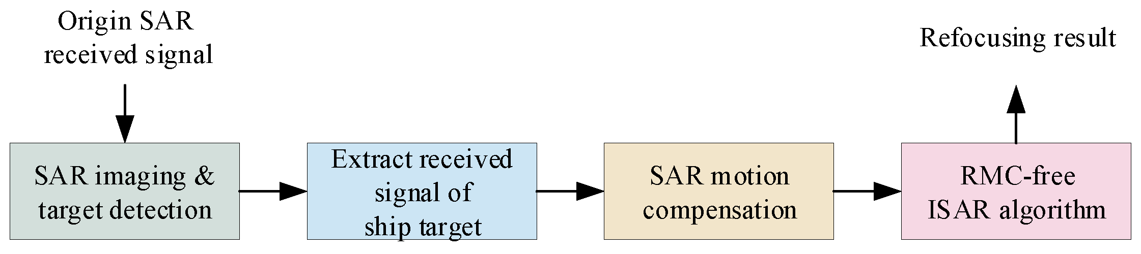
In the beginning, the overall framework of the proposed GEO SAR refocusing algorithm for ship targets with complex motion via CFSFD-based ISAR technique is introduced. This algorithm is designed based on the hybrid SAR/ISAR algorithm, and the step can be concluded as follows, as shown in Figure 1.

(1) 

Coarse SAR imaging and target detection.

(2) 

Extracting the received signal of the detected ship target.

(3) 

SAR motion compensation.

(4) 

RMC-free ISAR algorithm: Directly analyze azimuth Doppler frequency via CFSFD without RMC, and well-focused image can be obtained.

For steps (1) and (2), the methods proposed in [19] enables a constant false alarm rate detection with a high performance for ship targets, as well as a complete extraction of the received signal of each ship target. Therefore, this paper adopts the method presented in [19] as steps (1) and (2), and these two steps will not be further discussed. The remaining Section 2 focus on how to obtain a well-focused image starting from the extracted received signal through SAR motion compensation, followed by RMC-free ISAR algorithm.

2.2. Geometry and Signal Model

2.2.1. Geometry Model

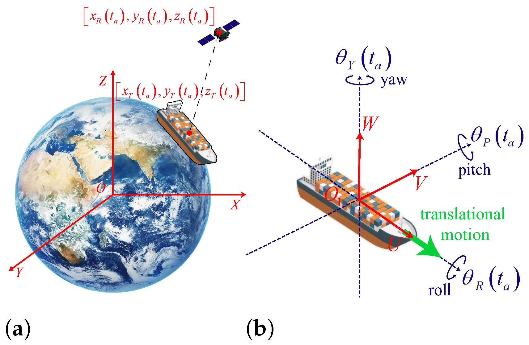
Before deriving the received signal model, the geometry model must be constructed. The satellite used in this paper is a GEO satellite designed to provide a long-time surveillance of South China Sea [9]. The orbit parameters are shown in

Table 2. Parameters of GEO SAR.

Semimajor	Eccentricity	Inclination	Argument of Perigee	RAAN	True Anomaly
42,150 km	0	${30}^{\circ }$	0	${180}^{\circ }$	$3^{\circ }$

. As shown in Figure 2a, the radar’s coordinates in the earth centered earth fixed (ECEF) coordinate system $O\text{-}XYZ$ can be written as

$$\begin{array}{c}{\mathbf{r}}_R\left(t_a\right)=\left[\begin{array}{c}{x}_R\left(t_a\right)\\ y_R\left(t_a\right)\\ z_R\left(t_a\right)\end{array}\right]=\left[\begin{array}{c}{x}_{R0}\\ y_{R0}\\ z_{R0}\end{array}\right]+\left[\begin{array}{c}\Delta x_R\left(t_a\right)\\ \Delta y_R\left(t_a\right)\\ \Delta z_R\left(t_a\right)\end{array}\right]\hfill \end{array}$$

(1)

where ${\mathbf{r}}_{R0}={\mathbf{r}}_R\left(0\right)$ is the initial position of radar. $\Delta {\mathbf{r}}_R\left(t_a\right)={\left[\Delta x_R\left(t_a\right),\Delta y_R\left(t_a\right),\Delta z_R\left(t_a\right)\right]}^T$ indicates the change in position induced by satellite motion, which can be calculated with the orbital elements.

Next, consider the complex motion of the ship target. Under the influence of wind and sea waves, the ship undergoes 3-D rotation: roll, pitch, and yaw. As shown by the blue arrows in Figure 2b, $O_1$ is the ship rotation center, U-axis is the longitudinal axis that runs fore and aft, V-axis is the transverse axis that runs side to side, and W-axis is the vertical axis that runs up and down. Roll, pitch and yaw are the oscillatory angular motions about U-axis, V-axis and W-axis, respectively. Roll, pitch, and yaw constitute the ship’s rotational motion. In addition, there is translational motion caused by the ship’s own propulsion, as shown by the green arrow in Figure 2b. Ship’s complex motion is the combination of the rotations and the translational motion. Hence, the coordinate of a scatterer p in the under ECEF can be written as

$$\begin{array}{c}{\mathbf{r}}_p\left(t_a\right)=\left[\begin{array}{c}{x}_p\left(t_a\right)\\ y_p\left(t_a\right)\\ z_p\left(t_a\right)\end{array}\right]=\mathbf{W}\left(t_a\right){\mathbf{u}}_p+{\mathbf{r}}_T\left(t_a\right)\hfill \\ {\mathbf{u}}_p=\left[\begin{array}{c}{u}_0\\ v_0\\ w_0\end{array}\right],{\mathbf{r}}_T\left(t_a\right)=\left[\begin{array}{c}{x}_T\left(t_a\right)\\ y_T\left(t_a\right)\\ z_T\left(t_a\right)\end{array}\right]=\Delta {\mathbf{r}}_T\left(t_a\right)+{\mathbf{r}}_{T0},\mathbf{W}\left(t_a\right)=\left[\begin{array}{ccc}{a}_{11}& a_{12}& a_{13}\\ a_{21}& a_{22}& a_{23}\\ a_{31}& a_{32}& a_{33}\end{array}\right]\hfill \end{array}$$

(2)

where ${\mathbf{r}}_T\left(t_a\right)$ is the coordinates of the ship rotation center in ECEF. ${\mathbf{r}}_{T0}={\mathbf{r}}_T\left(0\right)$ is the initial position of ship’s rotation center, and $\Delta {\mathbf{r}}_T\left(t_a\right)$ indicate the change in position induced by ship’s translational motion. ${\mathbf{u}}_p$ is the position of p under the target coordinate system $O_1\text{-}UVW$. $\mathbf{W}\left(t_a\right)$ is the rotation matrix, and the elements are

$$\begin{array}{c}{a}_{11}=cos{\theta }_{P}cos{\theta }_Y, a_{12}=-cos{\theta }_{P}sin{\theta }_Y, a_{13}=sin{\theta }_P\hfill \\ a_{21}=sin{\theta }_{R}sin{\theta }_{P}cos{\theta }_Y+cos{\theta }_{R}sin{\theta }_Y\hfill \\ a_{22}=-sin{\theta }_{R}sin{\theta }_{P}sin{\theta }_Y+cos{\theta }_{R}cos{\theta }_Y\hfill \\ a_{23}=-sin{\theta }_{R}cos{\theta }_P\hfill \\ a_{31}=-cos{\theta }_{R}sin{\theta }_{P}cos{\theta }_Y+sin{\theta }_{R}sin{\theta }_Y\hfill \\ a_{32}=cos{\theta }_{R}sin{\theta }_{P}sin{\theta }_Y+sin{\theta }_{R}cos{\theta }_Y\hfill \\ a_{33}=cos{\theta }_{R}cos{\theta }_P.\hfill \end{array}$$

(3)

where ${\theta }_R\left(t_a\right)$, ${\theta }_P\left(t_a\right)$, and ${\theta }_Y\left(t_a\right)$ are the rotation angles of roll, pitch and yaw, which can be evaluated by ship’s parameter and sea state. In previous research, these rotation angles are modeled as a sinusoidal function [31], which is

$${\theta }_{\mathrm{angle}}\left(t_a\right)=A_{\mathrm{angle}}sin\left(2\pi F_{\mathrm{angle}}{t}_a+{\vartheta }_{\mathrm{angle}}\right)+{\mathrm{\Theta }}_{\mathrm{angle}}$$

(4)

where $\mathrm{angle}=R,P,Y$, $A_{\mathrm{angle}}$ is the amplitude, $F_{\mathrm{angle}}$ is the rotation frequency, and ${\vartheta }_{\mathrm{angle}}$ is the initial phase. ${\mathrm{\Theta }}_{\mathrm{angle}}$ is the rotation angle that transforms $O_1\text{-}UVW$ coordinate system to $O\text{-}XYZ$ coordinate system.

The frequency and amplitude in (4) can be evaluated by the ship dynamics and the sea state (seeing the parts of sea keeping in [32]). The ship parameters used in this paper are shown in

Table 3. Ship parameters.

Waterplane Coefficient	Ship Length	Ship Width	Resistance of Roll	Depth of Draft	Natural Roll Period	Resistance of Pitch	Natural Pitch Period	Coefficient of Pitch
0.7	300 m	50 m	0.07	10 m	15 s	0.45	8 s	0.1

. They correspond to a large cargo vessel, which is one of the most common and representative targets in GEO SAR maritime surveillance. According to the Douglas offing state grade and the Beaufort scale, the ship rotation parameters in different sea states are shown in

Table 4. Ship rotation Parameters in different sea states.

Sea State	Wave Height	Wave Length	Roll Rotation Angle	Pitch Rotation Angle	Yaw Rotation Angle	Roll Period	Pitch Period	Yaw Period
3	1.5 m	15 m	5.3°	0.4°	0.2°	14.1 s	8.1 s	7.4 s
5	2.5 m	28 m	15°	1.7°	1°	12.0 s	6.7 s	7.5 s

. In this paper, sea states 3 and 5 are selected for analysis. This is because in lower sea states, the amplitude of complex motion induced by wind and waves on large vessels is small, and existing algorithms can already achieve refocusing [33]. In higher sea states, navigation becomes too dangerous, and ships typically stay in port rather than sail. Therefore, sea states 3 and 5 are chosen as the most representative conditions for maritime surveillance of ships with complex motion.

2.2.2. Signal Model

After extracting, the obtained signal is identical to the SAR received signal of the ship target after range compression. Hence, the received signal within GEO SAR image of the ship target with complex motion can be expressed as [14]

$$\begin{array}{c}\hfill S\left(t,t_a\right)=\sum _p{\sigma }_{p}sinc\left(B\left(t-{\displaystyle \frac{\lambda }{2\pi c}}{\phi }_p\left(t_a\right)\right)\right)exp\left(j{\phi }_p\left(t_a\right)\right)\end{array}$$

(5)

where ${\sigma }_p$ is the scatterer intensity, B is the bandwidth, $\lambda$ is the wavelength, and c is the speed of light. ${\phi }_p\left(t_a\right)$ is the phase function in azimuth dimension, which is

$$\begin{array}{c}\hfill {\phi }_p\left(t_a\right)={\displaystyle \frac{4\pi q{R}_p\left(t_a\right)}{\lambda }}\end{array}$$

(6)

where q is the ratio between the one-way propagation distance and slant range since the stop-go assumption in GEO SAR imaging no longer holds [9]. $R_p\left(t_a\right)$ is the slant range of the scatterer, which can be written as

$$\begin{array}{c}{R}_p\left(t_a\right)={\left|{\mathbf{r}}_R\left(t_a\right)-{\mathbf{r}}_p\left(t_a\right)\right|}_2.\hfill \end{array}$$

(7)

where ${\left|•\right|}_2$ is the 2-norm operator.

${\phi }_p\left(t_a\right)$ can be decomposed into three components [17,34]. That is

$$\begin{array}{c}\hfill {\phi }_p\left(t_a\right)={\displaystyle \frac{4\pi q}{\lambda }}{\left|{\mathbf{r}}_R\left(t_a\right)-{\mathbf{r}}_{T0}-\Delta {\mathbf{r}}_T\left(t_a\right)-\mathbf{W}\left(t_a\right){\mathbf{u}}_p\right|}_2\approx {\phi }_{1,p}\left(t_a\right)+{\phi }_{2,p}\left(t_a\right)+{\phi }_{3,p}\left(t_a\right)\end{array}$$

(8)

where ${\phi }_{1,p}\left(t_a\right)$ is the phase induced by radar motion, ${\phi }_{2,p}\left(t_a\right)$ is the phase induced by ship’s translational motion, and ${\phi }_{3,p}\left(t_a\right)$ is the phase induced by ship’s rotation, as shown as follows

$$\begin{array}{cc}\hfill & {\phi }_{1,p}\left(t_a\right)={\displaystyle \frac{4\pi q}{\lambda }}{\left|{\mathbf{r}}_R\left(t_a\right)-\left({\mathbf{r}}_{T0}+{\mathbf{W}}_0{\mathbf{u}}_p\right)\right|}_2\hfill \\ \hfill & {\phi }_{2,p}\left(t_a\right)={\displaystyle \frac{4\pi q}{\lambda }}{\left|{\mathbf{r}}_{R0}-\left({\mathbf{r}}_T\left(t_a\right)+{\mathbf{W}}_0{\mathbf{u}}_p\right)\right|}_2\hfill \\ \hfill & {\phi }_{3,p}\left(t_a\right)={\displaystyle \frac{4\pi q}{\lambda }}{\left|{\mathbf{r}}_{R0}-\left({\mathbf{r}}_{T0}+\mathbf{W}\left(t_a\right){\mathbf{u}}_p\right)\right|}_2\hfill \end{array}$$

(9)

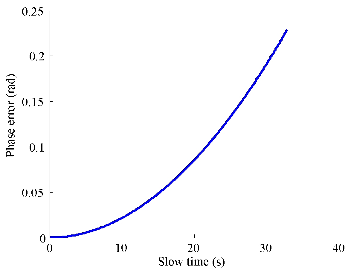
(8) holds when the phase error induced by the approximation is smaller than $\pi /2$, which is the basic assumption in this paper. In sea state 5 and with the radar parameters used in this paper, the phase error with respect to the synthetic aperture time is shown in Figure 3. It can be observed that when the synthetic aperture time is less than 32 s, the phase error is always smaller than $\pi /2$ and can therefore be neglected. Consequently, the sub-aperture time discussed in this paper should be no longer than 32 s. In addition, it should be noted that under milder sea states, the phase error would be even smaller, allowing for a longer permissible synthetic aperture time.

Let us discuss the three phase terms in detail. The first term ${\phi }_{1,p}\left(t_a\right)$ can be written as

$$\begin{array}{c}{\phi }_{1,p}\left(t_a\right)={\phi }_{\mathrm{SAR},\mathrm{p}}\left(t_a\right)+\Delta {\phi }_1\left(t_a\right)\hfill \\ {\phi }_{\mathrm{SAR},\mathrm{p}}\left(t_a\right)={\displaystyle \frac{2\pi q}{\lambda }}{\displaystyle \frac{V_E^2{\left(t_a-T_{p0}\right)}^2}{R_0}},\Delta {\phi }_1\left(t_a\right)={\displaystyle \frac{4\pi q}{\lambda }}{\left|{\mathbf{r}}_R\left(t_a\right)-{\mathbf{r}}_{T0}\right|}_2-{\displaystyle \frac{2\pi q}{\lambda }}{\displaystyle \frac{V_E^2{t}_a^2}{R_0}}\hfill \end{array}$$

(10)

where ${\phi }_{\mathrm{SAR},\mathrm{p}}\left(t_a\right)$ is a linear frequency modulation phase induced by the radar’s uniform motion perpendicular to RLOS. $V_E$ is the effective velocity of satellite, $T_{p0}$ is the aperture center moment (ACM) of scatterer p, and $R_0$ is the initial slant range. Another part is $\Delta {\phi }_1\left(t_a\right)$, which is the phase term induced by remaining motion of radar.

The second term ${\phi }_2\left(t_a\right)$ is the phase induced by translational motion. For different scatterers on the same target, it can be written as the same polynomial function [1,35]

$$\begin{array}{c}\hfill {\phi }_2\left(t_a\right)=\sum _n\Delta r_{T,n}{t}_a^n\end{array}$$

(11)

The third term ${\phi }_{3,p}\left(t_a\right)$ is induced by rotation, and it can be modeled as a sine-series functions [1,23]

$$\begin{array}{c}\hfill {\phi }_{3,p}\left(t_a\right)=\sum _n{A}_{n,p}sin\left({\omega }_{n,p}{t}_a+{\psi }_{n,p}\right)\end{array}$$

(12)

At this point, the received signal model of the ship target with complex motion within GEO SAR image is fully established.

2.3. SAR Motion Compensation

After extracting the received signal of the target, the SAR motion compensation needs to be implement. The SAR compensation function can be constructed as

$$\begin{array}{c}{H}_c\left(f_t,t_a\right)=exp\left(-j{\displaystyle \frac{\lambda f_t}{c}}\Delta {\phi }_1\left(t_a\right)\right)exp\left(-j\Delta {\phi }_1\left(t_a\right)\right)\hfill \end{array}$$

(13)

where $f_t$ is the range frequency corresponding to t. $\Delta {\phi }_1\left(t_a\right)$ can be obtained from (10). $V_E$ and ${\mathbf{r}}_R\left(t_a\right)$ can be obtained according to the prior information about SAR platform’s motion. ${\mathbf{r}}_{T0}$ and $T_{C0}$ can be obtained by target detection and estimation of the target’s position.

The received signal of ship target after SAR motion compensation is

$$\begin{array}{c}\hfill S_1\left(t,t_a\right)={\mathrm{IFT}}_t\left[{\mathrm{FT}}_t\left[S\left(t,t_a\right)\right]H_c\left(f_t,t_a\right)\right]=\sum _p{\sigma }_{p}sinc\left(B\left(t-{\displaystyle \frac{\lambda }{2\pi c}}{\phi }_{c,p}\left(t_a\right)\right)\right)exp\left(j{\phi }_{c,p}\left(t_a\right)\right)\end{array}$$

(14)

where ${\mathrm{IFT}}_t[•]$ and ${\mathrm{FT}}_t[•]$ are the inverse Fourier transform and the Fourier transform over t, respectively. ${\phi }_{c,p}\left(t_a\right)$ is the phase of scatterer p after SAR motion compensation, which is

$$\begin{array}{c}\hfill {\phi }_{c,p}\left(t_a\right)={\phi }_{\mathrm{SAR},\mathrm{p}}\left(t_a\right)+{\phi }_2\left(t_a\right)+{\phi }_{3,p}\left(t_a\right)\end{array}$$

(15)

2.4. ISAR Process

After SAR motion compensation, ISAR processing is required. The traditional ISAR algorithm is briefly introduced in Section 2.4.1, followed by an analysis of why this algorithm is difficult to apply to GEO SAR imaging of ship targets with complex motion. Specifically, the reason is the presence of higher-order space-varying range migration in the received signal. In Section 2.4.2, a RMC-free ISAR algorithm is proposed, which enables ISAR processing in the presence of higher-order space-varying range migration, thereby achieving GEO SAR refocusing for ship targets with complex motion.

2.4.1. Analysis of Traditional ISAR Algorithm

The first step in traditional ISAR technique is correcting the envelope shift in (14), and the signal after correction can be written as [29]

$$S_c\left(t,t_a\right)=\sum _p{\sigma }_{p}sinc\left(B\left(t-{\displaystyle \frac{\lambda {\phi }_{c,p0}}{2\pi c}}\right)\right)exp\left(j{\phi }_{c,p}\left(t_a\right)\right)$$

(16)

where ${\phi }_{c,p0}$ is the value of ${\phi }_{c,p}\left(t_a\right)$ at the initial time. Then, by using TFT to estimate the azimuth IF in $t_a=T_{\mathrm{IM}}$, the refocusing imaging result can be obtain as [36]

$$\begin{array}{c}H\left(t,f_a\right)={\displaystyle \sum _p}{\sigma }_{p}sinc\left(B\left(t-{\displaystyle \frac{\lambda {\phi }_{c,p0}}{2\pi c}}\right)\right)w_A\left(f_a-I{F}_p\left(T_{\mathrm{IM}}\right)\right)\hfill \end{array}$$

(17)

where $w_A$ is the envelope in azimuth dimension, which is determined in the process of TFT. $I{F}_p\left(T_{IM}\right)$ is the IF at $t_a=T_{\mathrm{IM}}$, which can be rewritten as

$$\begin{array}{c}I{F}_p\left(t_a\right)={\displaystyle \frac{d{\phi }_{c,p}\left(t_a\right)}{2\pi d{t}_a}}=I{F}_{\mathrm{SAR},\mathrm{p}}\left(t_a\right)+I{F}_2\left(t_a\right)+I{F}_{3,p}\left(t_a\right)\hfill \end{array}$$

(18)

where

$$\begin{array}{c}I{F}_{\mathrm{SAR},\mathrm{p}}\left(t_a\right)={\displaystyle \frac{d{\phi }_{\mathrm{SAR},\mathrm{p}}\left(t_a\right)}{2\pi d{t}_a}},I{F}_2\left(t_a\right)={\displaystyle \frac{d{\phi }_{2,p}\left(t_a\right)}{2\pi d{t}_a}},I{F}_{3,p}\left(t_a\right)={\displaystyle \frac{d{\phi }_{3,p}\left(t_a\right)}{2\pi d{t}_a}}\hfill \end{array}$$

(19)

The fundamental principle of ISAR imaging is that when the target can be considered a rigid body, the azimuth instantaneous Doppler frequency induced by rotation is proportional to the azimuth coordinate of the scatterer on the target [36]. That is

$$I{F}_{3,p}={\displaystyle \frac{d{\phi }_{3,p}\left(t_a\right)}{2\pi d{t}_a}}=\vartheta u_p$$

(20)

where $I{F}_{3,p}$ is the azimuth IF induced by rotation. $\vartheta$ is a proportional coefficient: $\vartheta ={\displaystyle \frac{2q{\omega }_0}{\lambda }}sin{\theta }_e$, where ${\omega }_0$ is the instantaneous angular velocity, ${\theta }_e$ is the angle between the radar line of sight and the instantaneous rotation axis of the target. $u_p$ is the azimuth coordinate of the scatterer in the target. In addition, when the target’s rotational velocity is high, the variation of $I{F}_{3,p}$ among different scatterers is much greater than that of $I{F}_{\mathrm{SAR},\mathrm{p}}$. Therefore, $I{F}_{\mathrm{SAR},\mathrm{p}}$ can be regarded as identical for all scatterers, and it is rewritten as $I{F}_{\mathrm{SAR}}$.

Based on the above derivation, it can be seen that in (17), the received signal of p will form a peak at $t={\displaystyle \frac{\lambda {\phi }_{c,p0}}{2\pi c}}$ and $\mathrm{\Omega }=I{F}_{\mathrm{SAR}}\left(T_{\mathrm{IM}}\right)+I{F}_2\left(T_{\mathrm{IM}}\right)+\vartheta u_p$. In (6), it can be seen that ${\phi }_{c,p0}$ is proportional to the slant range, indicating the position of the scatterer in range dimension. Meanwhile, $\vartheta u_p$ indicates the position of the scatterer in azimuth dimension. Thus, the peak in (17) is the imaging result of p.

The performance of such a RMC followed by TFT approach relies on the RMC algorithm, i.e., the transform from (14) to (16). However, the existing RMC algorithms are hard in correcting the space-varying fast-time delay induced by complex motion. In (14), the fast-time delay term is ${\displaystyle \frac{\lambda }{2\pi c}}{\phi }_{c,p}\left(t_a\right)$. It means that the position of the envelope of target’s received signal in fast-time dimension (range dimension) will change over $t_a$. This phenomenon is called range migration or envelope shift. The complex motion of ships consists of both translation and rotation, and in this subsection, their respective effects on range migration need to be analyzed separately. The fast-time delay term can be rewritten as

$$\begin{array}{c}\hfill \begin{array}{c}{t}_{RMC}\left(t_a\right)={\displaystyle \frac{\lambda }{2\pi c}}{\phi }_{c,p}\left(t_a\right)=t_{T,p}\left(t_a\right)+t_{R,p}\left(t_a\right)\hfill \end{array}\end{array}$$

(21)

where $t_{T,p}\left(t_a\right)$ is the fast-time delay induced by translational motion, and $t_{R,p}\left(t_a\right)$ is the fast-time delay induced by rotation. They can be rewritten as

$$\begin{array}{c}\hfill \begin{array}{c}{t}_{T,p}\left(t_a\right)={\displaystyle \frac{\lambda }{2\pi c}}{\displaystyle \sum _n}{r}_{T,n}{t}_a^n+{\displaystyle \frac{q}{c}}{\displaystyle \frac{V_E^2{\left(t_a-T_{p0}\right)}^2}{R_0}}\hfill \\ t_{R,p}\left(t_a\right)={\displaystyle \frac{\lambda }{2\pi c}}{\displaystyle \sum _n}{A}_{n,p}sin\left({\omega }_{n,p}{t}_a+{\psi }_{n,p}\right)\hfill \end{array}\end{array}$$

(22)

As mentioned in (16), for existing ISAR technique, RMC needs be implemented first. To achieve a high-resolution imaging, the remaining range migration should be less than the resolution in range dimension, i.e., ${\displaystyle \frac{c}{2B}}$. Consider the correction for $t_{T,p}\left(t_a\right)$ first. Since the extremely long distance of GEO SAR (42,150 km), $c{R}_0\gg V_E^2{T}_{p0}^2$ holds, and the variation of ${\displaystyle \frac{q}{c}}{\displaystyle \frac{V_E^2{\left(t_a-T_{p0}\right)}^2}{R_0}}$ for different scatterer is much smaller than ${\displaystyle \frac{c}{2B}}$ and can be neglect. Thus, $t_{T,p}\left(t_a\right)$ can be regard as the same for all scatterers. There are many ways can be used to handle such a range migration without space-variation, e.g., auto-correlation algorithm [20].

Next consider the correction for $t_{R,p}\left(t_a\right)$. This term varies for each scatterer and is related to the position of the scatterer, i.e., space-varying. In addition, it can be seen that $t_{R,p}\left(t_a\right)$ has third-order terms and higher. The widely applied SOKT [29] algorithm can correct the linear and quadratic term of the space-varying fast-time delay. After SOKT, the relative resident high-order fast-time delay induced by rotation is

$$\begin{array}{c}\hfill {\rho }_{RN,p}\left(t_a\right)={\displaystyle \frac{2B}{c}}\left(t_{R,p}\left(t_a\right)-a_{R0,p}-a_{R1,p}{t}_a-a_{R2,p}{t}_a^2\right)\end{array}$$

(23)

where $a_{R0,p}$, $a_{R1,p}$ and $a_{R2,p}$ is the polynomial coefficient of $t_{R,p}$. In traditional SAR/ISAR research, when the target rotation is small or synthetic aperture time is short, $t_{R,p}\left(t_a\right)$ can be approximated as linear or quadratic. However, for GEO SAR imaging for ship targets with complex motion, this assumption no longer holds due to the rotation and long synthetic aperture time. As analysis above, when the relative resident high-order fast-time delay induced by rotation is large than 1, it should be taken into account, meaning SOKT is inappropriate for such a signal. The critical condition can be written as

$$\begin{array}{cc}\hfill max\left[{\rho }_{RN,p}\left(t_a\right)\right]-min\left[{\rho }_{RN,p}\left(t_a\right)\right]<1,& t_a\in \left[0,T_S\right]\hfill \end{array}$$

(24)

where $T_S$ is the synthetic aperture time.

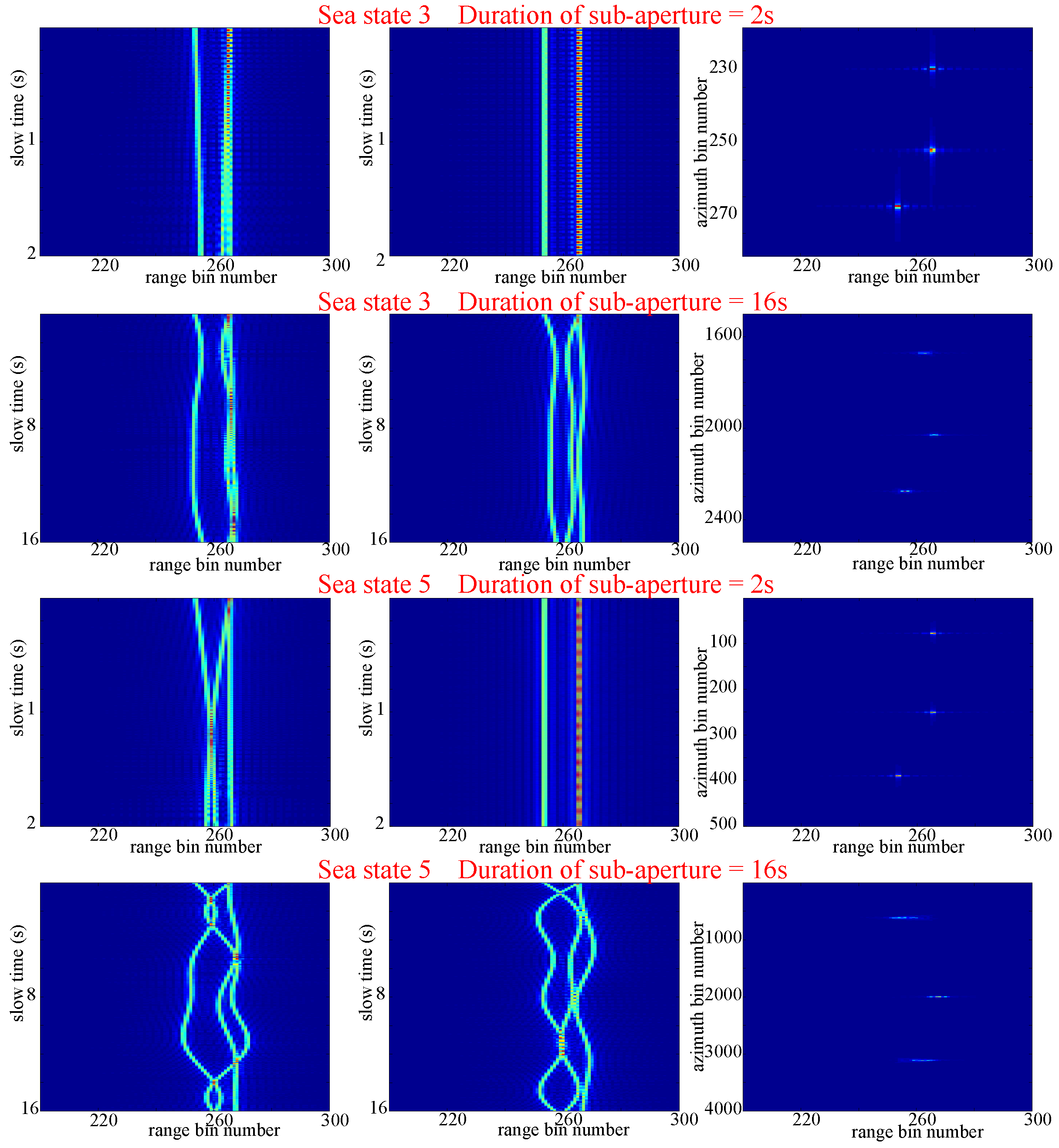
Whether (24) holds depends on many factors, including $T_S$, signal bandwidth, and the variation of ${\rho }_{RN,p}\left(t_a\right)$. The variation of ${\rho }_{RN,p}\left(t_a\right)$, in turn, is depended on factors such as the size and shape of the ship target, and the rotation velocity related on the sea state. Therefore, a specific imaging scenario is selected as an example for analysis, and a three-point target simulation is conducted. The reason for using such a target is that the simulation is designed to show the range migration of the scatterers’ received signals in different sea states and sub-aperture times. To better observe the range migration of the echoes, it is preferable to have as few scatterers as possible. The bandwidth is 70 MHz. The motion parameters are in Table 4. Since the ship’s rotation in Sea state 1 is too slight, the scenario in this condition was not simulated. The synthetic aperture time of GEO SAR in this paper is 80 s. For a target with complex motion, using the full synthetic aperture time is extremely hard and the sub-aperture needs to be used in existing research [37]. Thus, $T_S$ is substituting with the duration of sub-aperture, and the typical $T_S$ is tens of seconds. As shown in Figure 4, from left to right are the received signal of the ship target, the received signal of the ship target after SOKT and the refocusing imaging result, respectively. From up to down are the results in different sea state and $T_S$. It can be seen that when both the sea state is high and $T_S$ is long (for example, sea state 3 and $T_S$ = 16 s or sea state 5 and $T_S$ = 16 s), the impact of high-order fast-time delay induced by rotation arises, which cannot be corrected by SOKT and will blur the imaging result.

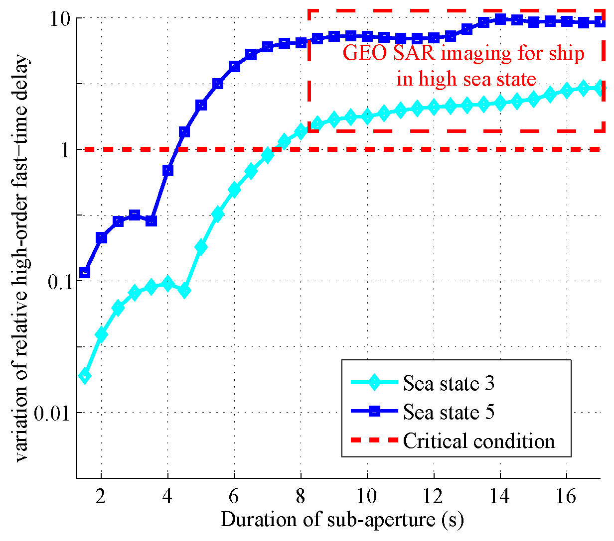
Figure 5 provides a more intuitive illustration of the relative high-order fast-time delay in different sea state and $T_S$. The critical condition in (24) is indicated by the red dashed. For example, in sea state 3 with $T_S$ = 2 s, the variation in relative high-order fast-time delay terms induced by rotation remains below 1, meaning it does not need to be considered. However, GEO SAR imaging requires a high SNR gain, necessitating a $T_S$ of several tens of seconds or longer. The high-order fast-time delay caused by the ship’s severe rotation is an essential factor to be considered, as indicated by the red dashed box.

In conclusion, when both the sea state is high and synthetic aperture time is long, the high-order fast-time delay induced by rotation cannot be neglected. In such a condition, the received signal of ship targets with complex motion cannot be corrected by the existing RMC algorithm, and the traditional ISAR algorithm is hard to be implemented.

2.4.2. RMC-Free ISAR Algorithm

As discussed in Section 2.4.1, the problem of the traditional ISAR algorithm in refocusing GEO SAR images of ship targets with complex motion lies in the fact that existing RMC algorithms cannot fully eliminate higher-order space-varying range migration. Meanwhile, TFT algorithms require complete range migration correction before azimuth IF estimation. Therefore, two possible approaches can address this issue: 1. Developing an advanced RMC algorithm capable of fully eliminating higher-order space-varying range migration. 2. Using a new algorithm that can estimate the azimuth IF even in the presence of range migration. The RMC-free ISAR algorithm proposed in this paper follows the second approach.

Consider a transform with an input signal $S_1\left(t,t_a\right)$ and an output $\mathrm{G}\left(t,t_a,\mathrm{\Omega }\right)$. In addition, this transform should also satisfy that each scatterer’s signal will form a peak in $t=\mathrm{\Gamma }{\phi }_{c,p}\left(t_a\right)$ and $\mathrm{\Omega }={\phi }_{c,p}^{\prime }\left(t_a\right)$, where $\mathrm{\Gamma }$ is an arbitrary nonzero constant.

Then, set a imaging moment $T_{\mathrm{IM}}$. Letting $S_2\left(t,\mathrm{\Omega }\right)=\mathrm{G}\left(t,T_{\mathrm{IM}},\mathrm{\Omega }\right)$, we have

$$\begin{array}{c}{S}_2\left(t,\mathrm{\Omega }\right)={\displaystyle \sum _p}{\sigma }_p{w}_r\left(t-\mathrm{\Gamma }{\phi }_{c,p}\left(T_{\mathrm{IM}}\right)\right)w_A\left(\mathrm{\Omega }-I{F}_p\left(T_{\mathrm{IM}}\right)\right)\hfill \end{array}$$

(25)

where $w_r(•)$ and $w_a(•)$ is the envelope function of the peak in $\mathrm{G}\left(t,t_a,\mathrm{\Omega }\right)$. From (6), it can be seen that ${\phi }_{c,p}\left(T_{\mathrm{IM}}\right)$ indicates the range position of the scatterer. Meanwhile, from (18) to (20), it can be seen that $I{F}_p\left(T_{\mathrm{IM}}\right)$ indicates the azimuth position of the scatterer. Thus, the peak in (25) is the imaging result of p. That is the RMC-free ISAR algorithm.

The key to this algorithm lies in the transform $\mathrm{G}\left(t,t_a,\mathrm{\Omega }\right)$. In Section 3, a transform that satisfies the above requirements, i.e., CFSFD, is introduced. By substituting CFSFD for $\mathrm{G}\left(t,t_a,\mathrm{\Omega }\right)$ in the above formulation, a well-focused image can be obtained, thereby achieving GEO SAR refocusing for targets with complex motion.

3. Complex Fast-Time Slow-Time Frequency Distribution

From (15), ${\phi }_{c,p}\left(t_a\right)$ can be rewritten as a joint sine-series-polynomial function

$$\begin{array}{c}\hfill {\phi }_{c,p}\left(t_a\right)=a_{0,p}+\sum _n{a}_n{t}_a^n+\sum _n{b}_{n,p}sin\left(c_{n,p}{t}_a+d_{n,p}\right)\end{array}$$

(26)

Thus, the received signal of ship target in such a scenario is a multicomponent 2-D joint sine-series-polynomial phase signal (2-D JSPS). Next, this section will introduce an algorithm for IF analysis of 2-D JSPS, namely the CFSFD. It can directly achieve azimuth IF analysis on a 2-D signal without any process like RMC, while has high accuracy and well suppression to cross-term interference even under low SNR and long synthetic aperture time.

3.1. Algorithm of Complex Fast-Time Slow-Time Frequency Distribution

First, consider a noise-free 1-D signal as

$$\begin{array}{c}\hfill S_{1\mathrm{D}}\left(t_a\right)=A_{0}exp\left(j\phi \left(t_a\right)\right)\end{array}$$

(27)

where $A_0$ is the amplitude, $\phi \left(t_a\right)$ is the phase function.

The results in [28] indicates that complex-lag time–frequency distribution (CTD) is an excellent time–frequency analysis algorithm for signals with nonlinear phase terms. The CTD of a 1-D signal can be expressed as

$$\begin{array}{c}\hfill \mathrm{CTD}\left(t_a,\omega \right)={\int }_{-\infty }^{\infty }\begin{array}{c}{S}_{1\mathrm{D}}\left(t_a+{\displaystyle \frac{\tau }{4}}\right)S_{1\mathrm{D}}^{*}\left(t_a-{\displaystyle \frac{\tau }{4}}\right)S_{1\mathrm{D}}^{-j}\left(t_a+j{\displaystyle \frac{\tau }{4}}\right)S_{1\mathrm{D}}^j\left(t_a-j{\displaystyle \frac{\tau }{4}}\right)e^{-j\omega \tau }d\tau \hfill \end{array}\end{array}$$

(28)

where $S_{1\mathrm{D}}\left(t_a+j\tau \right)$ is the 1-D signal with a complex lag $j\tau$. The complex lag of a 1-D signal is defined as

$$\begin{array}{c}\hfill S_{1\mathrm{D}}\left(t_a+j\tau \right)={\displaystyle \frac{1}{2\pi }}{\int }_{-\infty }^{\infty }F{T}_{\tau }\left[S_{1\mathrm{D}}\left(t_a+\tau \right)\right]e^{-\omega \tau }{e}^{j\omega t_a}d\omega .\end{array}$$

(29)

According to [25], (28) can be rewritten as

$$\begin{array}{c}\hfill \mathrm{CTD}\left(t_a,\omega \right)=A_0^2\delta \left(\omega -{\phi }^{\prime }\left(t_a\right)\right){\otimes }_{\omega }F{T}_{\tau }\left[exp\left(j{Q}_{\mathrm{CTD}}\left(t,\tau \right)\right)\right]\end{array}$$

(30)

where ${\otimes }_{\omega }$ is convolution over $\omega$, $F{T}_{\tau }\left[•\right]$ means Fourier transform (FT) over $\tau$. $Q_{\mathrm{CTD}}\left(t,\tau \right)$ is the spread factor, and it can be written as the series composed of derivatives with different orders

$$\begin{array}{c}\hfill Q_{\mathrm{CTD}}\left(t,\tau \right)={\phi }^{\left(5\right)}\left(t_a\right){\displaystyle \frac{{\tau }^5}{4^{4}5!}}+{\phi }^{\left(9\right)}\left(t_a\right){\displaystyle \frac{{\tau }^9}{4^{8}9!}}+\dots \end{array}$$

(31)

where ${\phi }^{\left(n\right)}\left(t_a\right)$ is n-th order derivative of the phase function. In (31), it can be seen that for the order less than four, derivative coefficients are equal to zero, meaning that CTD is completely immune to fourth-order and lower phase terms. Additionally, the fifth-order spread factor is ${\displaystyle \frac{1}{4^{4}5!}}\approx {\displaystyle \frac{1}{3\times {10}^4}}$, and the ninth-order spread factor is ${\displaystyle \frac{1}{4^{8}9!}}\approx {\displaystyle \frac{1}{2\times {10}^{10}}}\approx 0$. Hence, CTD still performs well for signals with fifth-order and above phase terms.

From the derivation of [25], (30) reaches its maximum when the following equation holds

$$\begin{array}{c}\hfill \omega ={\phi }^{\prime }\left(t_a\right)\end{array}$$

(32)

where ${\phi }^{\prime }\left(t_a\right)$ is the first-order derivative of the phase function, i.e., the IF. It means that the peak position of $\mathrm{CTD}\left(t_a,\omega \right)$ precisely lies on the function of the IF with respect to slow-time, and thus $\mathrm{CTD}\left(t_a,\omega \right)$ is the time–frequency distribution of $S_{1\mathrm{D}}\left(t_a\right)$.

Next consider a noise-free 2-D signal with space-varying fast-time delay as

$$\begin{array}{c}\hfill S\left(t, t_a\right)=A_{0}sinc\left[{\mathrm{\Gamma }}_1\left(t-{\mathrm{\Gamma }}_2\phi \left(t_a\right)\right)\right]exp\left(j\phi \left(t_a\right)\right)\end{array}$$

(33)

where ${\mathrm{\Gamma }}_1$ and ${\mathrm{\Gamma }}_2$ is two known constants.

CTD is designed for 1-D signal. Using CTD to handle $S\left(t, t_a\right)$ should choose a fast-time bin to decompose the 2-D signal into a 1-D signal, i.e., $S\left(T, t_a\right)$, where T is the processed fast-time bin. However, when the signal has a fast-time delay, doing so will cause some of the signal’s energy to fall outside the processed fast-time bin, leading to performance degradation. Therefore, we proposed a complex fast-time slow-time frequency distribution algorithm (CFSFD) that can directly perform time–frequency analysis on the 2-D signal with fast-time delay. CFSFD is defined as

$$\begin{array}{c}\hfill \begin{array}{c}\mathrm{CFSFD}\left(t, t_a, \mathrm{\Omega }\right)={\int }_{-\infty }^{\infty }\left[\begin{array}{c}W\left(\tau \right)S\left(t+{\mathrm{\Gamma }}_2\mathrm{\Omega }{\displaystyle \frac{\tau }{4}}, t_a+{\displaystyle \frac{\tau }{4}}\right)S^{*}\left(t-{\mathrm{\Gamma }}_2\mathrm{\Omega }{\displaystyle \frac{\tau }{4}}, t_a-{\displaystyle \frac{\tau }{4}}\right)\hfill \\ \times S^{-j}\left(t+{\mathrm{\Gamma }}_2\mathrm{\Omega }{\displaystyle \frac{\tau }{4}}, t_a+j{\displaystyle \frac{\tau }{4}}\right)S^j\left(t-{\mathrm{\Gamma }}_2\mathrm{\Omega }{\displaystyle \frac{\tau }{4}}, t_a-j{\displaystyle \frac{\tau }{4}}\right)\hfill \end{array}\right]e^{-j\mathrm{\Omega }\tau }d\tau \hfill \end{array}\end{array}$$

(34)

where $W\left(\tau \right)$ is the window function. $\mathrm{\Omega }$ is the IF. The 2-D signal with complex lag is

$$\begin{array}{c}\hfill \begin{array}{c}S\left(t+{\mathrm{\Gamma }}_2\mathrm{\Omega }{\displaystyle \frac{\tau }{4}},t_a+j{\displaystyle \frac{\tau }{4}}\right)={\displaystyle \frac{1}{2\pi }}{\int }_{-\infty }^{\infty }F{T}_{\tau }\left[S\left(t+{\mathrm{\Gamma }}_2\mathrm{\Omega }{\displaystyle \frac{\tau }{4}},t_a+{\displaystyle \frac{\tau }{4}}\right)\right]e^{-\omega {\displaystyle \frac{\tau }{4}}}{e}^{j\omega t_a}d\omega .\hfill \end{array}\end{array}$$

(35)

By substituting (33) and (35) into (34), it can be rewritten as (36)

$$\begin{array}{cc}\hfill & \mathrm{CFSFD}\left(t,t_a,\mathrm{\Omega }\right)=\hfill \\ & A_0^4{\int }_{-\infty }^{\infty }\left[\begin{array}{c}W\left(\tau \right)\left[sinc\left[{\mathrm{\Gamma }}_1\left(t+{\mathrm{\Gamma }}_2\mathrm{\Omega }{\displaystyle \frac{\tau }{4}}-{\mathrm{\Gamma }}_2\phi \left(t_a+{\displaystyle \frac{\tau }{4}}\right)\right)\right]exp\left(j\phi \left(t_a+{\displaystyle \frac{\tau }{4}}\right)\right)\right]\hfill \\ \times {\left[sinc\left[{\mathrm{\Gamma }}_1\left(t-{\mathrm{\Gamma }}_2\mathrm{\Omega }{\displaystyle \frac{\tau }{4}}-{\mathrm{\Gamma }}_2\phi \left(t_a-{\displaystyle \frac{\tau }{4}}\right)\right)\right]exp\left(j\phi \left(t_a-{\displaystyle \frac{\tau }{4}}\right)\right)\right]}^{*}\hfill \\ \times {\left[\begin{array}{c}{\displaystyle \frac{1}{2\pi }}{\int }_{-\infty }^{\infty }F{T}_{\tau }\left\{A_{0}sinc\left[{\mathrm{\Gamma }}_1\left(t+{\mathrm{\Gamma }}_2\mathrm{\Omega }{\displaystyle \frac{\tau }{4}}-{\mathrm{\Gamma }}_2\phi \left(t_a+{\displaystyle \frac{\tau }{4}}\right)\right)\right]\right\}{e}^{-\omega {\displaystyle \frac{\tau }{4}}}{e}^{j\omega t_a}d\omega \hfill \\ \times {\int }_{-\infty }^{\infty }F{T}_{\tau }\left[A_{0}exp\left(j\phi \left(t_a+{\displaystyle \frac{\tau }{4}}\right)\right)\right]e^{-\omega {\displaystyle \frac{\tau }{4}}}{e}^{j\omega t_a}d\omega \hfill \end{array}\right]}^{-j}\hfill \\ \times {\left[\begin{array}{c}{\displaystyle \frac{1}{2\pi }}{\int }_{-\infty }^{\infty }F{T}_{\tau }\left\{A_{0}sinc\left[{\mathrm{\Gamma }}_1\left(t-{\mathrm{\Gamma }}_2\mathrm{\Omega }{\displaystyle \frac{\tau }{4}}-{\mathrm{\Gamma }}_2\phi \left(t_a-{\displaystyle \frac{\tau }{4}}\right)\right)\right]\right\}{e}^{\omega {\displaystyle \frac{\tau }{4}}}{e}^{j\omega t_a}d\omega \hfill \\ \times {\int }_{-\infty }^{\infty }F{T}_{\tau }\left[A_{0}exp\left(j\phi \left(t_a-{\displaystyle \frac{\tau }{4}}\right)\right)\right]e^{\omega {\displaystyle \frac{\tau }{4}}}{e}^{j\omega t_a}d\omega \hfill \end{array}\right]}^j\hfill \end{array}\right]e^{-j\mathrm{\Omega }\tau }d\tau \hfill \end{array}$$

(36)

The peaks of (36) are located at (37), and the explanation is as follows.

$$\begin{array}{c}\hfill \begin{array}{c}t={\mathrm{\Gamma }}_2\phi \left(t_a\right)\hfill \\ \mathrm{\Omega }={\phi }^{\prime }\left(t_a\right).\hfill \end{array}\end{array}$$

(37)

(36) can be rewritten as

$$\begin{array}{c}\hfill \mathrm{CFSFD}\left(t,t_a,\mathrm{\Omega }\right)=A_0^4{\int }_{-\infty }^{\infty }W\left(\tau \right)M\left(t,\mathrm{\Omega },\tau \right)P\left(\tau \right)e^{-j\mathrm{\Omega }\tau }d\tau \end{array}$$

(38)

where $M\left(t,\mathrm{\Omega },\tau \right)$ is the envelope match term and $P\left(\tau \right)$ is the phase match term, which can be written as

$$\begin{array}{c}\begin{array}{c}M\left(t,\mathrm{\Omega },\tau \right)={\displaystyle \frac{1}{4{\pi }^2}}sinc\left[{\mathrm{\Gamma }}_1\left(t+{\mathrm{\Gamma }}_2\mathrm{\Omega }{\displaystyle \frac{\tau }{4}}-{\mathrm{\Gamma }}_2\phi \left(t_a+{\displaystyle \frac{\tau }{4}}\right)\right)\right]sin{c}^{*}\left[{\mathrm{\Gamma }}_1\left(t-{\mathrm{\Gamma }}_2\mathrm{\Omega }{\displaystyle \frac{\tau }{4}}-{\mathrm{\Gamma }}_2\phi \left(t_a-{\displaystyle \frac{\tau }{4}}\right)\right)\right]\hfill \\ \times {\left\{\int \begin{array}{c}F{T}_{\tau }\left\{A_{0}sinc\left[{\mathrm{\Gamma }}_1\left(t+{\mathrm{\Gamma }}_2\mathrm{\Omega }{\displaystyle \frac{\tau }{4}}-{\mathrm{\Gamma }}_2\phi \left(t_a+{\displaystyle \frac{\tau }{4}}\right)\right)\right]\right\}{e}^{-\omega {\displaystyle \frac{\tau }{4}}}{e}^{j\omega t_a}d\omega \hfill \end{array}\right\}}^{-j}\hfill \\ \times {\left\{\int \begin{array}{c}F{T}_{\tau }\left\{A_{0}sinc\left[{\mathrm{\Gamma }}_1\left(t-{\mathrm{\Gamma }}_2\mathrm{\Omega }{\displaystyle \frac{\tau }{4}}-{\mathrm{\Gamma }}_2\phi \left(t_a-{\displaystyle \frac{\tau }{4}}\right)\right)\right]\right\}{e}^{\omega {\displaystyle \frac{\tau }{4}}}{e}^{j\omega t_a}d\omega \hfill \end{array}\right\}}^j\hfill \end{array}\hfill \\ \begin{array}{c}P\left(\tau \right)=exp\left(j\phi \left(t_a+{\displaystyle \frac{\tau }{4}}\right)\right){exp}^{*}\left(j\phi \left(t_a-{\displaystyle \frac{\tau }{4}}\right)\right)\hfill \\ \times {\left[\int F{T}_{\tau }\left[A_{0}exp\left(j\phi \left(t_a+{\displaystyle \frac{\tau }{4}}\right)\right)\right]e^{-\omega {\displaystyle \frac{\tau }{4}}}{e}^{j\omega t_a}d\omega \right]}^{-j}{\left[\int F{T}_{\tau }\left[A_{0}exp\left(j\phi \left(t_a-{\displaystyle \frac{\tau }{4}}\right)\right)\right]e^{\omega {\displaystyle \frac{\tau }{4}}}{e}^{j\omega t_a}d\omega \right]}^j\hfill \end{array}\hfill \end{array}$$

(39)

Consider $\int P\left(\tau \right)e^{-j\mathrm{\Omega }\tau }d\tau$, the FT of phase term. The integration is exactly the same as (28). From (32), $\int P\left(\tau \right)e^{-j\mathrm{\Omega }\tau }d\tau$ reaches its maximum when $\mathrm{\Omega }={\phi }^{\prime }\left(t_a\right)$. On the other hand, it can be seen from (39) that $M\left(t,\mathrm{\Omega },\tau \right)$ consists of four sinc functions with time delay. In other words, it is a real-valued envelope function and does not affect the phase. It can also be observed that the maximum value of $M\left(t,\mathrm{\Omega },\tau \right)$ is $1/4{\pi }^2$. Therefore, the following inequality holds

$$\begin{array}{c}{\int }_{-\infty }^{\infty }M\left(t,\mathrm{\Omega },\tau \right)P\left(\tau \right)e^{-j\mathrm{\Omega }\tau }d\tau \le {\int }_{-\infty }^{\infty }{\displaystyle \frac{1}{4{\pi }^2}}P\left(\tau \right)e^{-j\mathrm{\Omega }\tau }d\tau \hfill \end{array}$$

(40)

Hence, only when $M\left(t,\mathrm{\Omega },\tau \right)$ reaches its maximum, can $\int M\left(t,\mathrm{\Omega },\tau \right)P\left(\tau \right)e^{-j\mathrm{\Omega }\tau }d\tau$ reaches its maximum. In addition, the maximum of $M\left(t,\mathrm{\Omega },\tau \right)$ can be reached when zero equals the variable in sinc functions, i.e., $t+{\mathrm{\Gamma }}_2\mathrm{\Omega }{\displaystyle \frac{\tau }{4}}-{\mathrm{\Gamma }}_2\phi \left(t_a+{\displaystyle \frac{\tau }{4}}\right)$ and $t-{\mathrm{\Gamma }}_2\mathrm{\Omega }{\displaystyle \frac{\tau }{4}}-{\mathrm{\Gamma }}_2\phi \left(t_a-{\displaystyle \frac{\tau }{4}}\right)$. By rewritten $\phi \left(t_a+{\displaystyle \frac{\tau }{4}}\right)$ as $\phi \left(t_a+{\displaystyle \frac{\tau }{4}}\right)=\phi \left(t_a\right)+{\phi }^{\prime }\left(t_a\right){\displaystyle \frac{\tau }{4}}+\Delta \phi \left(t_a\right)$, the variable in sinc functions can be rewritten as

$$\begin{array}{c}t+{\mathrm{\Gamma }}_2\mathrm{\Omega }{\displaystyle \frac{\tau }{4}}-{\mathrm{\Gamma }}_2\phi \left(t_a+{\displaystyle \frac{\tau }{4}}\right)=\left(t-{\mathrm{\Gamma }}_2\phi \left(t_a\right)\right)+{\mathrm{\Gamma }}_2\left(\mathrm{\Omega }-{\phi }^{\prime }\left(t_a\right)\right){\displaystyle \frac{\tau }{4}}+{\mathrm{\Gamma }}_2\Delta \phi \left(t_a\right)\hfill \\ t-{\mathrm{\Gamma }}_2\mathrm{\Omega }{\displaystyle \frac{\tau }{4}}-{\mathrm{\Gamma }}_2\phi \left(t_a-{\displaystyle \frac{\tau }{4}}\right)=\left(t-{\mathrm{\Gamma }}_2\phi \left(t_a\right)\right)-{\mathrm{\Gamma }}_2\left(\mathrm{\Omega }-{\phi }^{\prime }\left(t_a\right)\right){\displaystyle \frac{\tau }{4}}-{\mathrm{\Gamma }}_2\Delta \phi \left(t_a\right)\hfill \end{array}$$

(41)

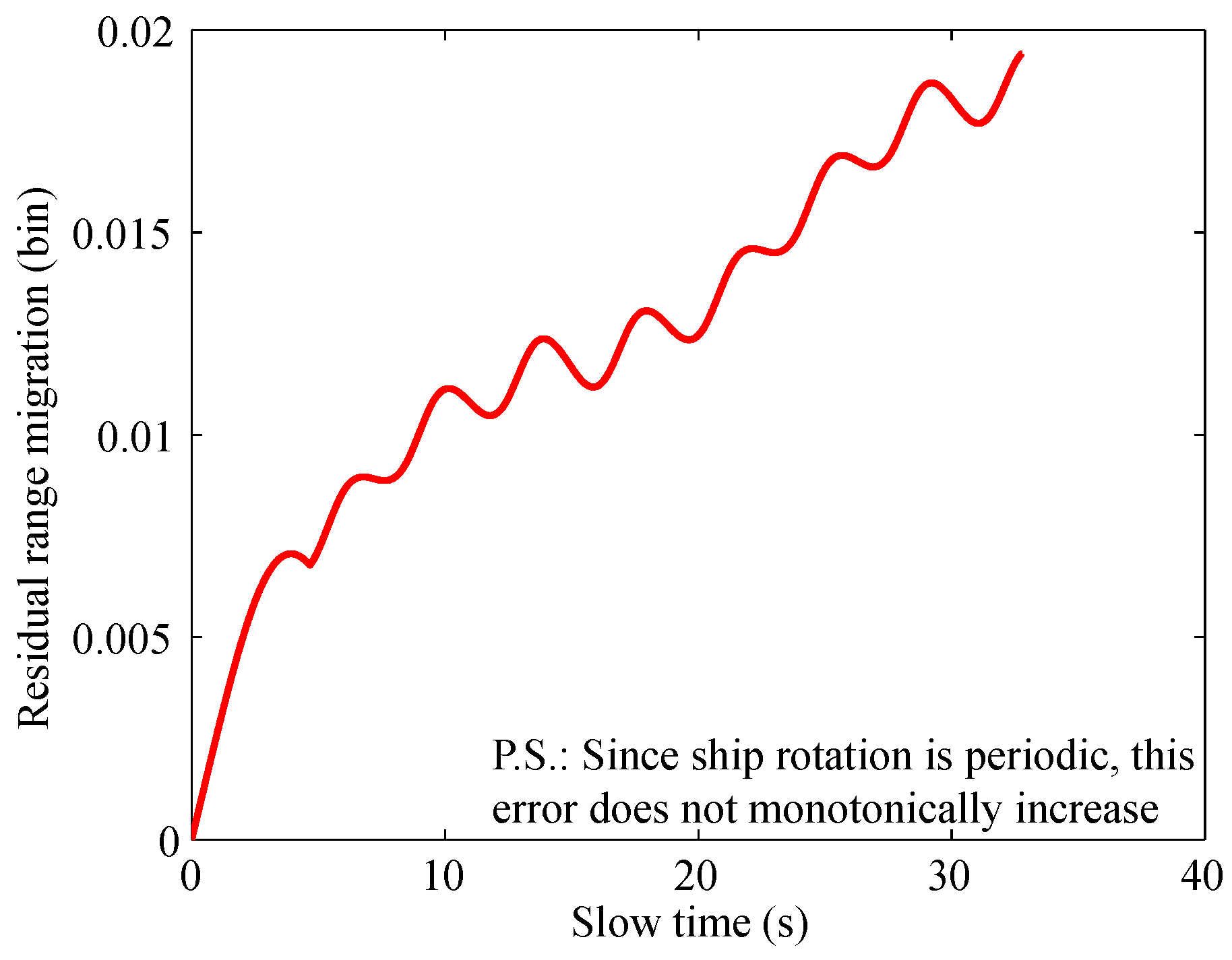
where $\Delta \phi \left(t_a\right)$ is high-order phase error. This phase error corresponds to the residual range migration, which causes the metric $M\left(t,\mathrm{\Omega },\tau \right)$ to deviate from its peak value. Although the signal can be considered to remain within the same range bin when the residual range migration is less than half of a range bin, for high-precision imaging, we recommend that the residual range migration should less than one-tenth of a range bin. In sea state 5 and with the radar parameters used in this paper, the residual range migration induced by $\Delta \phi \left(t_a\right)$ is much smaller than one-tenth of a range bin (the length of range bin is 2 m) and can be neglected, as shown in Figure 6.

In (41), when $t={\mathrm{\Gamma }}_2\phi \left(t_a\right)$, the first term equal to 0. When $\mathrm{\Omega }={\phi }^{\prime }\left(t_a\right)$, the second term equal to 0. Thus, when (37) holds, the variable in sinc functions equal to 0, $M\left(t,\mathrm{\Omega },\tau \right)$ equals to $1/4{\pi }^2$. Since $\int P\left(\tau \right)e^{-j\mathrm{\Omega }\tau }d\tau$ reaches its maximum in $\mathrm{\Omega }={\phi }^{\prime }\left(t_a\right)$, the equality in (40) holds, and (36) reaches it maximum. That is (36) reaches it maximum in (37).

By comparing (37) with (32), it can be seen that the peaks of $\mathrm{CFSFD}\left(t,t_a,\mathrm{\Omega }\right)$ is no longer located on the function of the IF with respect to slow-time, but rather on the function of the IF and fast-time delay with respect to slow-time. Therefore, CFSFD is not a traditional slow-time frequency distribution. Instead, it is a fast-time slow-time frequency distribution. The advantages of CFSFD are as follows and will be verified in next subsection.

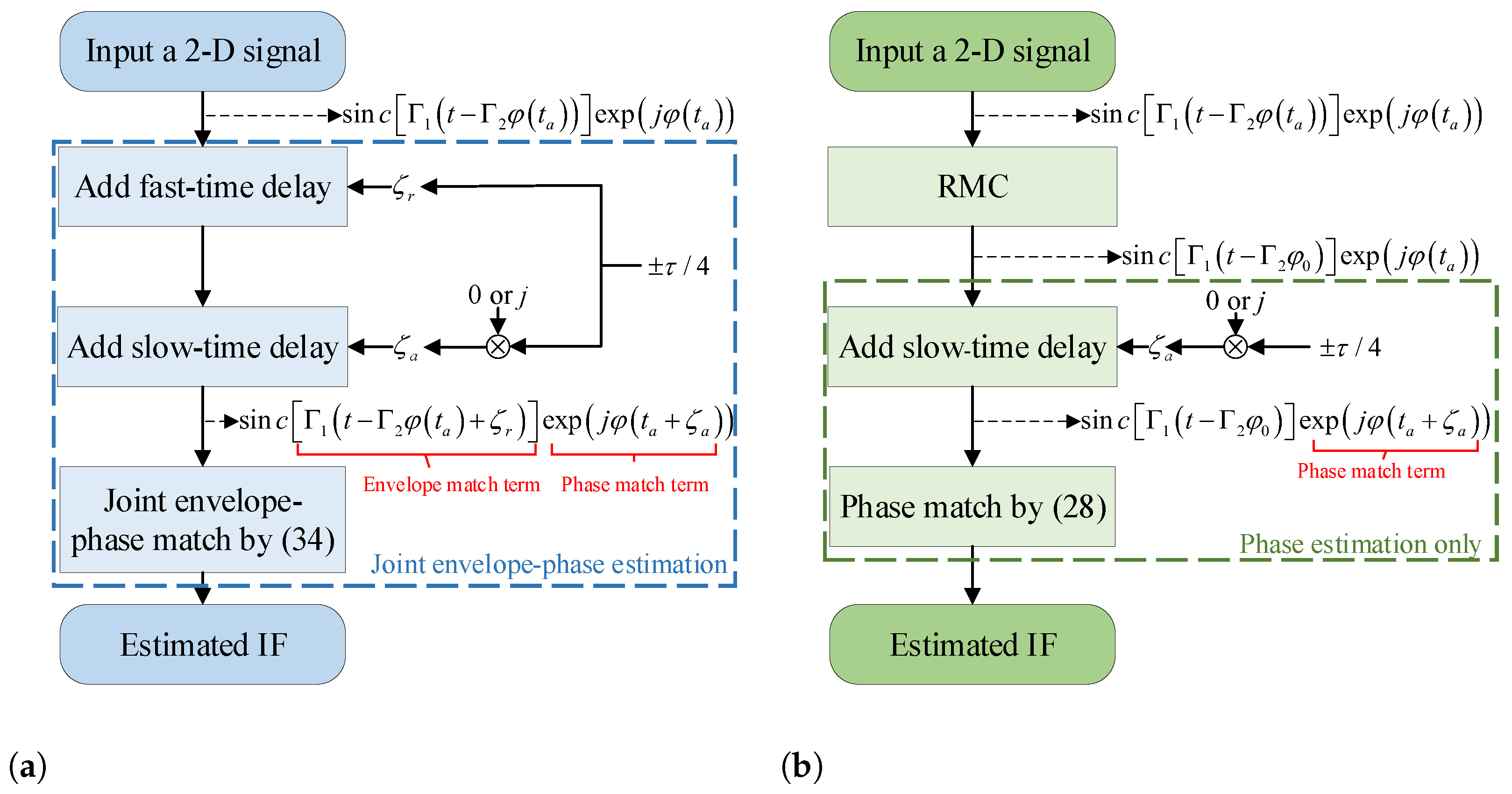
• Figure 7a shows the flowchart of the proposed CFSFD, while Figure 7b illustrates the flowchart of the method based on traditional TFT. It can be seen that, compared with the traditional TFT, the CFSFD introduces an additional fast-time delay to match the range migration term, i.e., the envelope match term in the figure. When the fast-time delay and the range migration are matched, the envelope match term reaches its maximum value while the range migration is eliminated. Therefore, CFSFD gains the ability to directly process signals with fast-time delay without RMC.
• When $\mathrm{\Omega }$ does not match the signal’s IF, both the envelope and phase terms of CFSFD decay rapidly. In contrast, existing TFT only experience phase term decay. As a result, CFSFD exhibits faster decay outside the peak, improving estimation accuracy.
• In (33), when the components’ phases are different, their envelopes are different, too. Therefore, for multicomponent signal, the envelope terms of CFSFD only match the envelope of one component under a set of t and $\mathrm{\Omega }$, i.e., envelope terms reach its peak. Other components, due to the mismatch of their envelopes, will have their amplitudes suppressed by the envelope terms of CFSFD. Thus, CFSFD exhibits good cross-term suppression performance.
• The phase match terms of CFSFD are same as that of CTD, allowing CFSFD to inherit the excellent performance in handling high-order phase terms.

3.2. Numerical Example

Consider a three-components 2-D JSPS, the phase function of each component is

$$\begin{array}{c}\mathrm{Signal}1:{\phi }_1\left(t_a\right)=40sin\left(2\pi t_a/30\right)+9sin\left(2\pi t_a/25\right)+sin\left(2\pi t_a/20\right)+0.01t_a^2+0.2t_a\hfill \\ \mathrm{Signal}2:{\phi }_2\left(t_a\right)=-30sin\left(2\pi t_a/30\right)+15sin\left(2\pi t_a/25\right)-2sin\left(2\pi t_a/20\right)+0.01t_a^2+0.2t_a\hfill \\ \mathrm{Signal}3:{\phi }_3\left(t_a\right)=20sin\left(2\pi t_a/30\right)-12sin\left(2\pi t_a/25\right)-3sin\left(2\pi t_a/20\right)+0.01t_a^2+0.2t_a.\hfill \end{array}$$

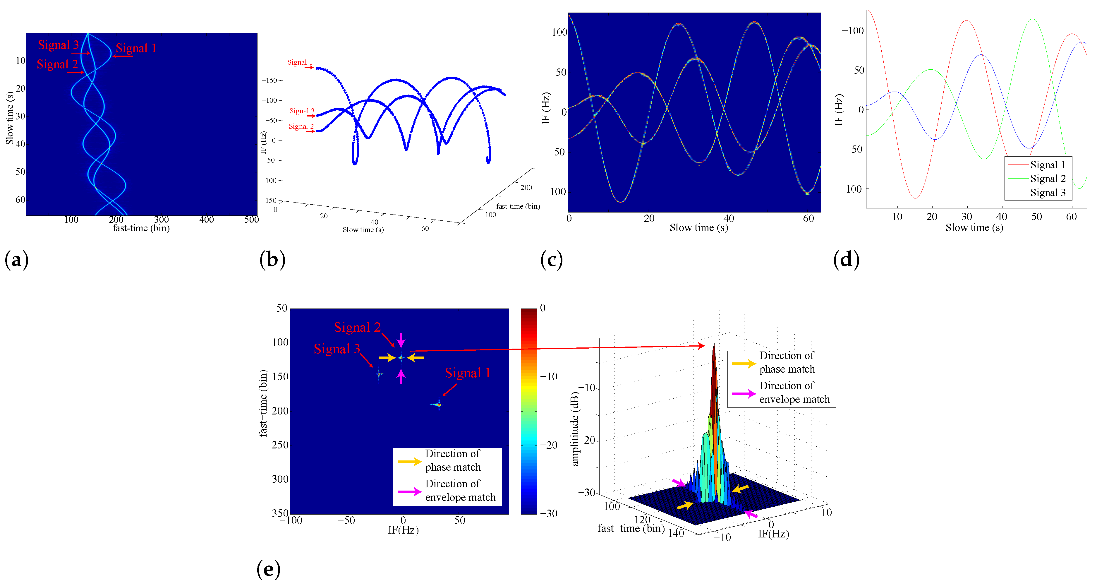
For simplification, the three components are called Signal 1, Signal 2 and Signal 3, respectively. The amplitude of each component is the same. The sampling rate in fast-time dimension is 150 MHz, the pulse repetition frequency (PRF) is 250 Hz, ${\mathrm{\Gamma }}_1=70$ Hz, and ${\mathrm{\Gamma }}_2=1/70$. The three components signal is shown in Figure 8a. The unit of fast-time is bin, and the length of the bin is equal to the resolution in fast-time dimension. By implementing CFSFD, the spectrum is obtained. However, $\mathrm{CFSFD}\left(t,t_a,\mathrm{\Omega }\right)$ is a function with three variables and cannot be printed in the paper directly. Therefore, we normalize $\mathrm{CFSFD}\left(t,t_a,\mathrm{\Omega }\right)$, and then the points larger than −10 dB are shown in Figure 8b. It can be seen that these points form three curves, which corresponds to the IF and fast-time delay of the three components.

By projecting the CFSFD spectrum onto the fast-time dimension, the time–frequency spectrum can be obtained as shown in Figure 8c. The theoretical IF of the three components are shown in Figure 8d, and it is same as the projection of CFSFD spectrum. It can also be observed that there are no cross-terms at the overlap of the three components, showing the cross-term suppression ability of CFSFD.

To illustrate how CFSFD achieve envelope and phase matched more vividly, a slice in $t_a=8$ s from Figure 8b is presented in Figure 8e, i.e., $\mathrm{CFSFD}\left(t,t_a=8\mathrm{s},\mathrm{\Omega }\right)$. It can be seen that three components form three peaks corresponding to their IF and fast-time delay in 8 s, respectively. Taking the peak of Signal 2 as example, the yellow arrow represents the direction of envelope match, meaning that as t gets closer to ${\mathrm{\Gamma }}_2\phi \left(t_a\right)$, the envelope gradually matches, and the function reaches its maximum value along this row. The purple arrow represents the direction of phase match, meaning that as $\mathrm{\Omega }$ gets closer to the IF of signal, the phase gradually matches, and the function reaches its maximum value along this column. Only when the phase and envelope match simultaneously, resulting in the overall maximum value of the function.

3.3. Accuracy and Concentration Analysis

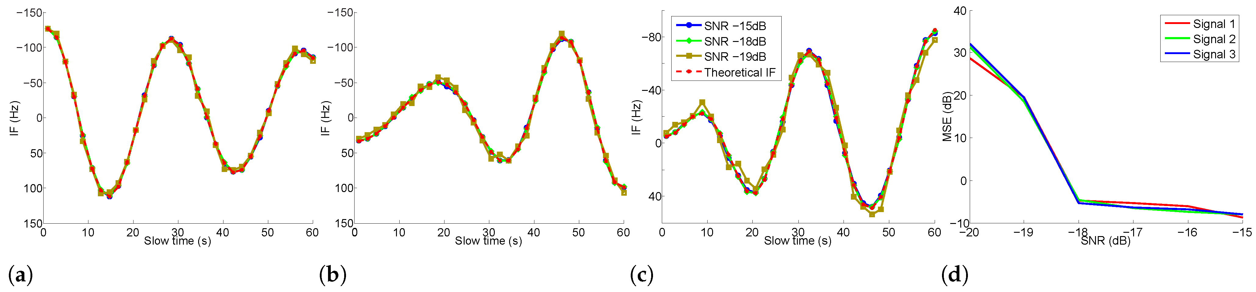
To show the high accuracy and good concentration of CFSFD in the low SNR, the three-components signal is mixed with additive white Gaussian noise (AWGN). The SNR is set as −20 dB to −15 dB. The estimated IF of the three components are shown in Figure 9a, b and c, respectively. The red line is the theoretical IF for reference. It can be seen that when SNR $\ge -18$ dB, the estimated IF with the two SNR are almost overlap to the theoretical IF, showing the high accuracy of the proposed algorithm under the low SNR. When SNR $<-19$ dB the errors of estimation increase sharply as shown in Figure 9d. Thus, the threshold SNR of CFSFD is −19 dB.

The concentration of TFT is defined as [28]

$$\begin{array}{c}\hfill M_{\mathrm{con}}={\displaystyle \frac{\int \int {\left|TFT\left(t,\omega \right)\right|}^{4}d\omega dt}{{\left(\int \int {\left|TFT\left(t,\omega \right)\right|}^{2}d\omega dt\right)}^2}}\end{array}$$

(42)

where $TFT\left(t,\omega \right)$ is a TFT’s time–frequency spectrum. The larger the $M_{\mathrm{con}}$ is, the better the TFT’s concentration is.

CFSFD is a fast-time slow-time frequency transform with three variables, and it is concentration cannot be calculated by (42). For ease of comparison, we use the projection of CFSFD spectrum onto the the fast-time dimension (like Figure 8c) to calculate the concentration of CFSFD.

Table 5. Concentration of different algorithms ($\times {10}^{-7}$).

Spectrogram	SPWVD	CTD	CFSFD
0.020	0.029	0.199	3.791

presents the concentration of CFSFD and several mainstream TFTs with SNR = −15 dB. It can be seen the concentration of CFSFD is greater than that of these TFTs.

4. Detailed Steps of Proposed GEO SAR Refocusing Algorithm

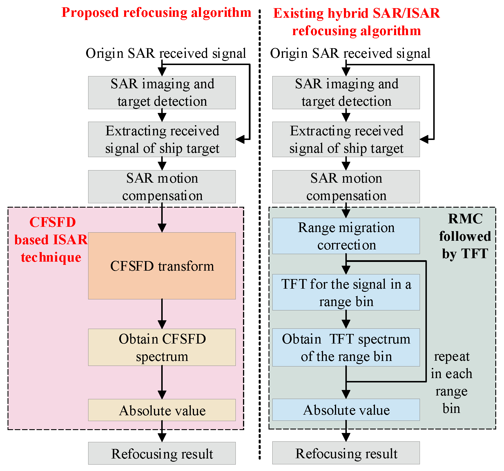
Based on the analysis above, the GEO SAR refocusing algorithm for ship target with complex motion via CFSFD-based ISAR technique is proposed. The steps of the proposed refocusing algorithm and the comparison with existing SAR/ISAR refocusing algorithm are shown in Figure 10. It can be seen that the proposed algorithm uses CFSFD to achieve IF estimation for ISAR imaging, replacing the traditional IF estimation approach of RMC followed by TFT. This algorithm is RMC-free, since CFSFD is a joint phase-envelope estimation. The detailed steps are provided below.

(1) 

SAR imaging and target detection.

(2) 

Extracting the received signal of the ship target, denoting as $S(t,t_a)$. The detailed steps can refer to [9,10,19].

(3) 

Implement SAR motion compensation for $S(t,t_a)$, and denote the signal after compensation as $S_1(t,t_a)$. The detailed steps are in Section 2.3.

(4) 

Implement CFSFD on $S_1(t,t_a)$, and obtain the spectrum $\mathrm{CFSFD}\left(t,t_a,\mathrm{\Omega }\right)$

(5) 

Set $T_{\mathrm{IM}}$, which is the time of imaging. The algorithm of optimal time selection refers to [33]. Get the spectrum at $t_a=T_{\mathrm{IM}}$, i.e., $S_2\left(t,\mathrm{\Omega }\right)=\mathrm{CFSFD}\left(t,T_{\mathrm{IM}},\mathrm{\Omega }\right)$

(6) 

Let $S_3\left(t,\mathrm{\Omega }\right)=\left|H_3\left(t,\mathrm{\Omega }\right)\right|$, which is the refocusing result.

It should be reiterated that the applicability of the proposed algorithm requires the errors in (8) and (41) to be negligible. Under the parameters used in this paper, both equations hold within a 32 s sub-aperture time. When the parameters change, the threshold need to be recalculated.

5. Results

In this section, a simulated experiment and an experiment on spaceborne SAR data are presented. The two experiments are conducted on the personal computer equipped with 13th Gen Inter(R) (address: 2200 Mission College Blvd. Santa Clara, CA, USA, 95054-1549) Core(TM) i7-13700K CPU, Intel(R) UHD Graphics 770 (128 MB) GPU and 32 GB RAM.

5.1. Simulated Experiment

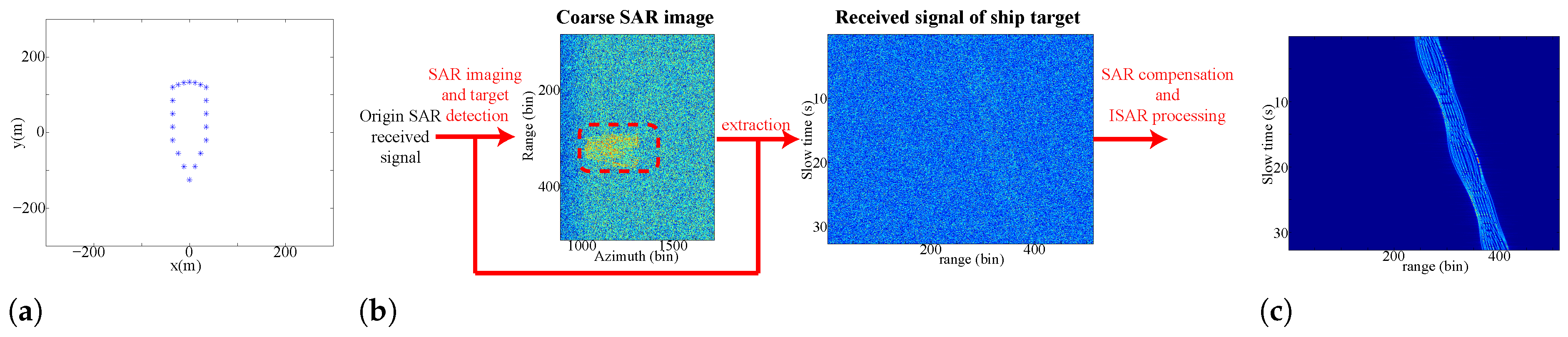
In this subsection, a simulated experiment is conducted to show the performance of the proposed GEO SAR refocusing algorithm for ship target with complex motion via CFSFD-based ISAR technique. The ship target model consisted of scatterers with the same scattering intensity is used, as shown in Figure 11a. The ship target undergoes complex motion, including a forced 3-D rotation induced by the wave under Level 5 sea state and a 20 knots translational motion along the trajectory driven by its own propulsion. The full synthetic aperture time is 80 s and the used sub-aperture time is 32 s. More parameters of the experiment are shown in

Table 6. Radar parameters of simulated experiment.

Carrier Frequency	Bandwidth	Pulse Width	Sub-Aperture Time	Pulse Repetition Frequency	Antenna Aperture	Incidence Angle	SNR (After Range Compression)
2 GHz	70 MHz	10 us	32 s	250 Hz	40 m	${17}^{\circ }$	−15 dB

and

Table 7. Ship target motion parameter of simulated experiment.

Velocity	Acceleration	Maximum Roll Rotation Angle	Roll Period	Maximum Pitch Rotation Angle	Pitch Period	Maximum Yaw Rotation Angle	Yaw Period
20 knots	0.2 knots/s	15°	12 s	1.7°	6.7 s	1°	7.5 s

. After SAR imaging and target detection, the received signal of the ship target is extracted, as shown in Figure 11b. For clarity, the received signal of the ship target with noise removal is also given in Figure 11c, and obviously this signal is a multicomponent 2-D JSPS. The SNR in this simulation is set to −15 dB, following the first helicopter platform-based equivalent GEO SAR experiment in [38]. It should be noted that the antenna aperture and gain of the satellite used in this paper differ from those in [38]. Thus, the SNR is also different, although the radar equation used for calculation is the same.

After SAR motion compensation, the ISAR technique based on CFSFD is used to obtain refocusing imaging result. For comparison, the algorithms of RMC followed by TFT are also employed, which are the most commonly used ISAR refocusing algorithm in existing research [11,20]. SOKT is currently the highest-order KT-type algorithm, which is capable of handling space-varying range migration [29]. Therefore, SOKT is selected as the RMC algorithm in the comparison experiments. Meanwhile, several commonly used time–frequency distributions including Spectrogram, SPWVD, and CTD are adopted as the TFT algorithms in the comparison experiments, as they perform well for first-order, second-order, and fourth-order polynomial phases, respectively [28]. Finally, the comparison algorithms used in this paper is SOKT-Spectrogram, SOKT-SPWVD, and SOKT-CTD.

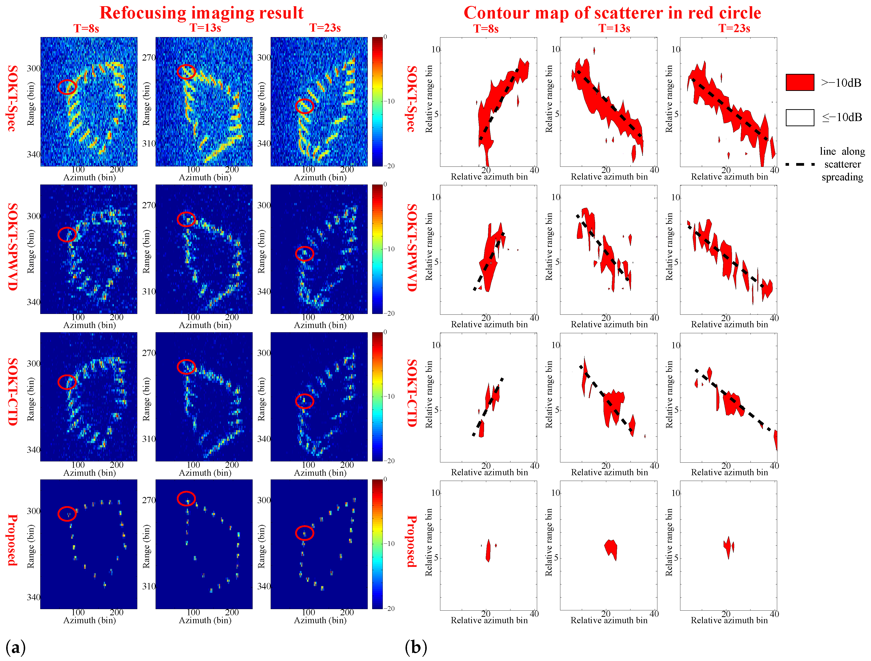
The refocusing results of different algorithms are shown in Figure 12a. From left to right are the refocusing results in $T=8$ s, $T=13$ s and $T=23$ s, respectively. From up to down are the results of SOKT-Spectrogram, SOKT-SPWVD, SOKT-CTD and proposed algorithm, respectively. It can be seen that the refocusing results of proposed algorithm is the clearest.

To better observe the blurring of the refocusing results, we selected a scatterer at each imaging time and plotted its imaging result as a contour map, as shown in Figure 12b. The contour map correspond to the scatterers indicated by red circle in Figure 12a. In the contour maps of SOKT-Spectrogram, SOKT-SPWVD and SOKT-CTD, it can seen that the scatterer is blurred in both range and azimuth dimension, appearing as a line (indicated by the black dash line) rather than a point. In the contour maps of proposed algorithm, we can see that the scatterer is well-focused in both azimuth and range dimension and have no distortion, appearing as a point rather than a line.

Image entropy [18,20] and impulse response width (IRW) [17] are two commonly used quantitative metrics for evaluating ISAR image quality. The image entropy is defined as

$$E_I=-\sum _1^M\sum _1^N{\displaystyle \frac{I^2\left(n,m\right)}{P}}ln{\displaystyle \frac{I^2\left(n,m\right)}{P}}$$

(43)

where $E_I$ is the image entropy, and $I(n,m)$ is the image. n and m are the range bin number and the azimuth bin number, respectively. The image has N azimuth bins and M range bins. $P={\displaystyle \sum _1^M}{\displaystyle \sum _1^N}{I}^2\left(n,m\right)$. The IRW is the peak width of the scatterer’s imaging result along a given dimension. Since the direction of line of scatterer spreading not align with either the range or azimuth dimensions, the IRW in the two dimensions cannot describe the degree of blurred and distortion. Thus, we use the IRW along the line of scatterer spreading as the indicators. The image entropy and the IRW along the line of scatterer spreading are shown in

Table 8. Image entropies of Figure 12 in simulation.

	T = 8 s	T = 13 s	T = 23 s
SOKT-Spec	9.44	9.44	9.45
SOKT-SPWVD	7.88	7.91	7.97
SOKT-CTD	7.51	7.66	7.42
Proposed	6.74	6.84	6.79

and

Table 9. IRW (bin) along line of scatterer spreading in Figure 12 in simulation.

	T = 8 s	T = 13 s	T = 23 s
SOKT-Spec	25.4	34.1	42.8
SOKT-SPWVD	13.0	26.1	41.3
SOKT-CTD	10.9	25.4	36.2
Proposed	2.2	5.8	5.1

, respectively. It can be seen that the proposed algorithm has minimum image entropies and minimum IRW. Therefore, the proposed algorithm performs best in GEO SAR refocusing for ship target with complex motion.

5.2. Experiment on Spaceborne SAR Data

In this subsection, a set of low earth orbit (LEO) SAR data is used to verify the effectiveness of the proposed algorithm in practical maritime surveillance scenarios. The altitude of the satellite is about 600 km with a Ku-band spaceborne radar. The used sub-aperture time is 10 s.

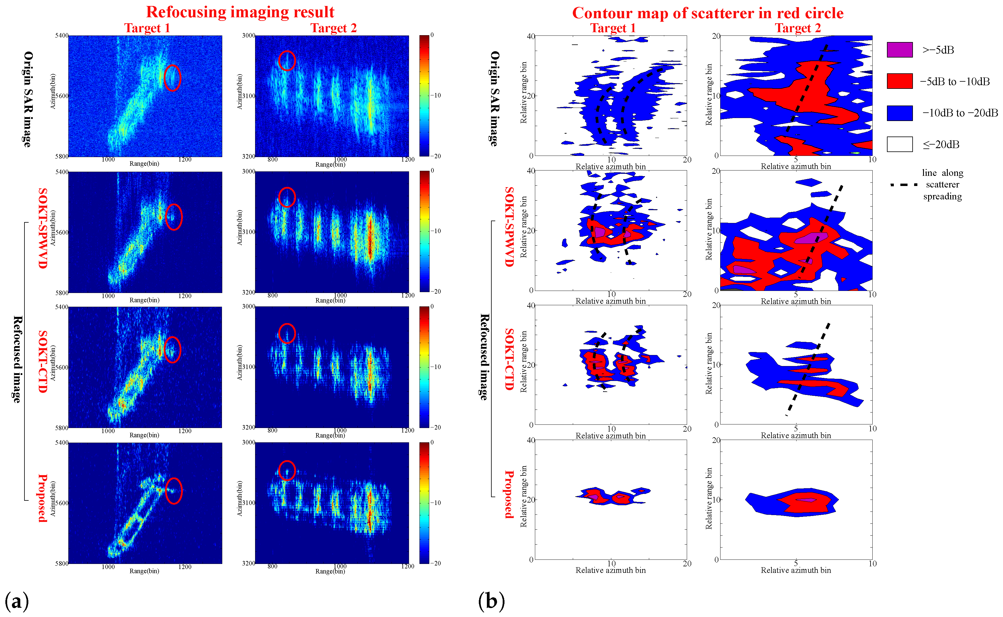
First, the received signal of two ship targets with complex motion is extracted from the origin SAR data, and the SAR imaging results of the two targets are shown in the first row of Figure 13a. It can be seen that the imaging results of the ship targets are severely blurred. To more clearly observe these imaging results, several strong scatterers on the ship target were selected for analysis, as indicated by the red circles. The profiles corresponding to the red circles are shown in Figure 13b. It can be seen that in the original SAR image, these scatterers exhibit severe distortion, distributed along the black dashed lines rather than appearing as point-like scatterers. This phenomenon indicates that the complex motion of the ship target was not compensated, which is similar to the simulation experiment result of SOKT-Spectrogram algorithm (seeing Figure 12a).

Subsequently, different refocusing algorithms are applied to refocus the two targets. Since the SOKT-Spectrogram algorithm has already been verified in simulation experiments to be ineffective for handling such a target, resulting in poor performance, it is not included in the comparison. The refocusing results obtained using SOKT-SPWVD, SOKT-CTD, and the proposed algorithm are shown in the second, third, and fourth rows of Figure 13a, respectively. It can be observed that the three algorithm all improve the imaging quality of the refocused results, while the proposed algorithm achieves the best performance: the refocused ship targets obtained using the comparison algorithms still exhibit blurred boundaries. In contrast, the refocused ship targets using the proposed algorithm not only show clear and distinct boundaries but also allow the ship’s structures to be more clearly identified. The contour map of scatterers indicated by the red circles are also shown in Figure 13b. It can be seen that the scatterers still exhibit distortion in the refocusing results of SOKT-SPWVD and SOKT-CTD, while the scatterer of the proposed algorithm appear as a point.

The image entropy of these imaging results and the IRW along the line of scatterer spreading are shown in

Table 10. Image entropies of Figure 13 in experiment on spaceborne SAR data.

Algorithm	Target 1	Target 2
Origin SAR image	6.65	5.82
SOKT-SPWVD	4.43	4.18
SOKT-CTD	4.38	3.99
Proposed	2.95	3.15

and

Table 11. IRW (bin) along line of scatterer spreading in Figure 13 in experiment on spaceborne SAR data.

Algorithm	Target 1	Target 2
Origin SAR image	24.0	8.2
SOKT-SPWVD	8.4	7.3
SOKT-CTD	8.0	6.6
Proposed	4.8	3.5

, respectively. The proposed algorithm has minimum image entropies and minimum IRW. In conclusion, the real data experiment shows that the proposed algorithm achieves the best performance in GEO SAR refocusing for ship target with complex motion.

6. Discussion

6.1. Discussion on Simulated Experiment

In the simulated experiment, the proposed algorithm and three algorithms for comparison are used to refocused the ship target with complex motion. In Figure 12a, it is obvious that the refocusing result of the proposed algorithm are clearest, with minimum image entropy and minimum IRW, indicating its best performance.

Figure 12b, on the other hand, illustrates the underlying reason why the proposed algorithm outperforms the others. In Figure 12b, it can be seen that the scatterers appear as a line rather than a point in the results of SOKT-Spectrogram, SOKT-SPWVD and SOKT-CTD. This line extends across both the range bins and azimuth bins, indicating that the scatterer is blurred in both the two dimensions. The presence of blurred in the range dimension suggests that the SOKT algorithm cannot completely eliminate the space-varying fast-time delay, and the remaining range migration make the scatterers distorted. This phenomenon is consistent with the analysis presented in Section 2.4 of this paper, which points out that existing RMC algorithms is difficult to deal with the range migration in received signals from targets with complex motion. In addition, it can be observed that the defocusing in the results of SOKT-Spectrogram is more severe than that in the results of SOKT-SPWVD and SOKT-CTD. This is because the Spectrogram algorithm is affected by the second-order phase term and higher.

In the refocusing results of the proposed algorithm, the scatterer form a circular spot rather than a line, and shows a significantly reduced span in both the range and azimuth dimensions. This phenomenon indicates the refocusing results are well-focused in both azimuth and range dimension and have no distortion. These results validate the ability of the CFSFD algorithm to perform frequency analysis on received signals from complex motion targets with range migration, consistent with the theory and experiments presented in Section 3. It also demonstrates the effectiveness of the GEO SAR refocusing algorithm for ship target with complex motion via the CFSFD-based ISAR technique.

Finally, the resolution is discussed. The image obtained using the ISAR or hybrid SAR/ISAR algorithm have a range resolution of ${\displaystyle \frac{c}{2B}}$ and an azimuth resolution of ${\displaystyle \frac{\lambda }{2\theta }}$ [39], where $\theta$ is the rotation angle in azimuth dimension. Thus, the range resolution of the experiment is 2.14 m. After accounting for the radar’s incidence angle, the resolution is 2.14/$sin{17}^{\circ }=7.33$ m. In Figure 12a, it can be observed that the range dimension corresponds to the lengthwise direction of the ship. The ship occupies 40 bins ($40\times 7.33=293.2$ m) in the range dimension, consistent with the actual ship length 300 m. The azimuth dimension corresponds to the ship’s width direction. Thus, $\theta$ is the roll rotation angle ${15}^{\circ }$, and the azimuth resolution is 0.29 m. The ship image occupies 155 bins ($155\times 0.29=44.5$ m) in the azimuth dimension, consistent with the actual ship width 50 m.

6.2. Discussion on Experiment on Spaceborne SAR Data

In this experiment, the received signals of two real ships are used instead of point scatterers’ simulated received signals. From the results of this experiment, it is evident that the refocusing results of proposed algorithm is the clearest, with the minimum IRW and minimum image entropy, indicating that the proposed algorithm performs best in this experiment. Then, the equivalence between this LEO SAR experiments and GEO SAR imaging for ship target with complex motion is analyzed as follows.

First, let us discuss the differences between LEO SAR and GEO SAR from a theoretical perspective. (1) to (12) in the paper derive the received echo model for GEO SAR. It can be observed that applying the same derivation process to LEO SAR requires only two modifications: In (6), the ratio q equals 1 for LEO SAR; the approximation in (8) needs to be re-evaluated for LEO SAR parameters. q is a constant ratio, and its specific value does not affect the characteristics of the received signal. The approximation in (8) also holds under the LEO SAR parameters used in this paper, as the sub-aperture time is significantly shorter (the shorter the sub-aperture time, the smaller the approximation error becomes). Therefore, under the condition that (8) remains valid, the LEO SAR signal can substitute for the GEO SAR signal to verify the proposed algorithm. In other words, only when the approximation in (8) no longer holds do the effects of the ultra-long synthetic aperture time in GEO SAR become significant, making LEO SAR unsuitable as a substitute.

Next, whether imaging ship targets with complex motion using GEO SAR or LEO SAR, the main challenge lies in the fact that the ship’s complex motion introduces high-order space-varying range migration in the received signal. Existing algorithms are unable to handle such a signal, whereas the proposed algorithm can. This is precisely the advantage of the proposed algorithm. In the results of SOKT-Spectrogram, SOKT-SPWVD and SOKT-CTD shown in Figure 13b, the scatterers are blurred in both the range and azimuth dimensions, consistent with the results in simulation experiments. The defocusing in range dimension indicates that SOKT cannot fully eliminate range migration, demonstrating the presence of higher-order range migration caused by the target’s complex motion. Meanwhile, the proposed algorithm successfully achieves well-focused imaging. Therefore, this experiment effectively verifies the key advantage of the proposed algorithm: its capability to handle signals with high-order space-varying range migration caused by the target’s complex motion.

In summary, although the LEO SAR experiment can only partially reflect the conditions of the GEO SAR scenario, it can still verify the advantages of the proposed algorithm: its ability to process signals containing high-order space-varying range migration caused by complex motion and obtain well-focused image, which cannot be achieved by the other compared algorithms.

7. Conclusions

In this paper, we focus on the GEO SAR refocusing of ship targets with complex motion, and a GEO SAR refocusing algorithm for ship target with complex motion via CFSFD-based ISAR technique is proposed. This hybrid SAR/ISAR refocusing algorithm uses CFSFD-based ISAR technique to replace the traditional RMC followed by TFT approach, and can obtain clear refocusing result when simultaneously encountering low SNR, long synthetic aperture time, and high-order space-varying range migration. Simulation and real data experiment validate the effectiveness of the proposed algorithm.

References

1. Yu, J.; Yu, Z.; Li, C. GEO SAR Imaging of Maneuvering Ships Based on Time–Frequency Features Extraction. IEEE Trans. Geosci. Remote Sens. 2022, 60, 5226321. [Google Scholar] [CrossRef] [Scilit]
2. Monti, M.; Guarnieri, A.M.; Pelliccia, F.; Renga, A. Geostationary Interferometric SAR: Orbit Design and Control Implementation. IEEE Trans. Geosci. Remote Sens. 2025, 63, 5211017. [Google Scholar] [CrossRef] [Scilit]
3. Monti, M.; Monti-Guarnieri, A.; Petrushevsky, N.; Prati, C.; Graziano, D.; Renga, A.; Pelliccia, F.; Blasone, G.P.; Montuori, A. Geostationary SAR: Orbit Design and Optimization. In Proceedings of the 15th European Conference on Synthetic Aperture Radar, Munich, Germany, 23–26 April 2024; pp. 895–900. [Google Scholar]
4. Tang, F.; Ji, Y.; Zhang, Y.; Dong, Z.; Wang, Z.; Zhang, Q.; Zhao, B.; Gao, H. Drifting Ionospheric Scintillation Simulation for L-band Geosynchronous SAR. IEEE J. Sel. Top. Appl. Earth Obs. Remote Sens. 2024, 17, 842–854. [Google Scholar] [CrossRef] [Scilit]
5. Sun, Z.; Sun, H.; An, H.; Li, Z.; Wu, J.; Yang, J. Trajectory Optimization for Maneuvering Platform Bistatic SAR with Geosynchronous Illuminator. IEEE Trans. Geosci. Remote Sens. 2024, 62, 5203715. [Google Scholar] [CrossRef] [Scilit]
6. Li, C.; Zhang, Q.; Liu, J.; Han, G.; Liu, B.; Duan, C.; Lu, Z. Subretrograde Geosynchronous SAR: Parameter Design and Performance Analysis. IEEE J. Sel. Top. Appl. Earth Obs. Remote Sens. 2024, 17, 68–83. [Google Scholar]
7. Hu, C.; Li, Y.; Chen, Z.; Liu, F.; Zhang, Q.; Monti-Guarnieri, A.V.; Hobbs, S.; Anghel, A.; Datcu, M. Distributed Spaceborne SAR: A Review of Systems, Applications, and the Road Ahead. IEEE Geosci. Remote Sens. Mag. 2025, 13, 329–361. [Google Scholar] [CrossRef] [Scilit]
8. Cui, C.; Dong, X.; Chen, Z. GEO SA-BSAR Synchronization and MTI Algorithm Based on Direct Signal and Clutter Subspace. IEEE J. Sel. Top. Appl. Earth Obs. Remote Sens. 2024, 17, 4368–4378. [Google Scholar] [CrossRef] [Scilit]
9. Zhu, X.; Jiang, Y.; Liu, Z.; Zhang, Y.; Wang, Y.; Hua, Q. Division and Focusing of Multiple Moving Ship Targets for GEO SAR via MFDFrFT Spectrum Analysis. IEEE Trans. Geosci. Remote Sens. 2024, 62, 5217816. [Google Scholar] [CrossRef] [Scilit]
10. Cao, R.; Wang, Y.; Zhao, B.; Lu, X. Ship Target Imaging in Airborne SAR System Based on Automatic Image Segmentation and ISAR Technique. IEEE J. Sel. Top. Appl. Earth Obs. Remote Sens. 2021, 14, 1985–2000. [Google Scholar] [CrossRef] [Scilit]
11. Cao, R.; Wang, Y.; Sun, S.; Zhang, Y. Three Dimension Airborne SAR Imaging of Rotational Target with Single Antenna and Performance Analysis. IEEE Trans. Geosci. Remote Sens. 2022, 60, 5225417. [Google Scholar] [CrossRef] [Scilit]
12. Qi, X.; Zhang, Y.; Jiang, Y.; Liu, Z.; Yang, C. MosReformer: Reconstruction and Separation of Multiple Moving Targets for Staggered SAR Imaging. Remote Sens. 2023, 15, 4911. [Google Scholar] [CrossRef] [Scilit]
13. Wang, Y.; Zhao, B. Inverse Synthetic Aperture Radar Imaging of Nonuniformly Rotating Target Based on the Parameters Estimation of Multicomponent Quadratic Frequency-Modulated Signals. IEEE Sens. J. 2015, 15, 4053–4061. [Google Scholar] [CrossRef] [Scilit]
14. Zhu, X.; Jiang, Y.; Liu, Z.; Chen, R.; Qi, X. A Novel ISAR Imaging Algorithm for Maneuvering Targets. IEEE Geosci. Remote Sens. Lett. 2022, 19, 4502905. [Google Scholar] [CrossRef] [Scilit]
15. Shi, S.; Zhang, H.; Deng, Y.; Ren, M. Increase the Coherent Processing Interval for SAR Focusing of Maneuvering Ships by Data Resampling. IEEE Trans. Geosci. Remote Sens. 2024, 62, 5210322. [Google Scholar] [CrossRef] [Scilit]
16. Jiang, Y.; Wei, J.; Liu, Z.; Zhang, Y.; Wang, Y. A Novel Three-Dimension Imaging Algorithm Based on Trajectory Association of ISAR Image Sequence. IEEE Geosci. Remote Sens. Lett. 2023, 20, 4000405. [Google Scholar] [CrossRef] [Scilit]
17. Guo, J.; Yang, W.; Qi, W.; Deng, J.; Zeng, H.; Chen, J.; Wang, Y.; Ji, W.; Wang, W. Refocusing of Rotating Ships in Spaceborne SAR Imagery Based on NLCS Principle. IEEE Trans. Geosci. Remote Sens. 2024, 62, 5207015. [Google Scholar] [CrossRef] [Scilit]
18. Yang, S.; Li, S.; Fan, H.; Liu, Y. High-Resolution ISAR Imaging of Maneuvering Targets Based on Azimuth Adaptive Partitioning and Compensation Function Estimation. IEEE Trans. Geosci. Remote Sens. 2023, 61, 5222115. [Google Scholar] [CrossRef] [Scilit]
19. Martorella, M.; Pastina, D.; Berizzi, F.; Lombardo, P. Spaceborne Radar Imaging of Maritime Moving Targets with the Cosmo-SkyMed SAR System. IEEE J. Sel. Top. Appl. Earth Obs. Remote Sens. 2014, 7, 2797–2810. [Google Scholar] [CrossRef] [Scilit]
20. Qian, G.; Wang, Y. Monostatic-Equivalent Algorithm via Taylor Expansion for BiSAR Ship Target Imaging. IEEE Trans. Geosci. Remote Sens. 2023, 61, 5200919. [Google Scholar] [CrossRef] [Scilit]
21. Chen, R.; Jiang, Y. Hybrid SAR-ISAR Imaging for Space Target via 2-D Spectrum and SIHR with Spaceborne Radar. IEEE Trans. Aerosp. Electron. Syst. 2024, 60, 2106–2127. [Google Scholar] [CrossRef] [Scilit]
22. Long, Y.; Zhao, F.; Zheng, M.; Zhao, L.; He, W. An Unambiguous Imaging Method of Moving Target for Maritime Scenes with Spaceborne High-Resolution and Wide-Swath SAR. IEEE Trans. Geosci. Remote Sens. 2022, 60, 5224519. [Google Scholar] [CrossRef] [Scilit]
23. Chen, V.C.; Miceli, W.J. Time-Varying Spectral Analysis for Radar Imaging of Manoeuvring Targets. Iee Proc. Radar Sonar Navig. 1998, 145, 262–268. [Google Scholar] [CrossRef] [Scilit]
24. Stankovic, L.; Thayaparan, T.; Dakovic, M.; Popovic-Bugarin, V. Micro-Doppler Removal in the Radar Imaging Analysis. IEEE Trans. Aerosp. Electron. Syst. 2013, 49, 1234–1250. [Google Scholar] [CrossRef] [Scilit]
25. Stankovic, L. Time-Frequency Distributions with Complex Argument. IEEE Trans. Signal Process. 2002, 50, 475–486. [Google Scholar] [CrossRef] [PubMed]
26. Cornu, C.; Stankovic, S.; Ioana, C.; Quinquis, A.; Stankovic, L. Generalized Representation of Phase Derivatives for Regular Signals. IEEE Trans. Signal Process. 2007, 55, 4831–4838. [Google Scholar] [CrossRef] [Scilit]
27. Stankovic, S.; Orovic, I.; Ioana, C. Effects of Cauchy Integral Formula Discretization on the Precision of If Estimation: Unified Approach to Complex-Lag Distribution and Its Counterpart l-Form. IEEE Signal Process. Lett. 2009, 16, 327–330. [Google Scholar] [CrossRef] [Scilit]
28. Orovic, I.; Orlandic, M.; Stankovic, S.; Uskokovic, Z. A Virtual Instrument for Time-Frequency Analysis of Signals with Highly Nonstationary Instantaneous Frequency. IEEE Trans. Instrum. Meas. 2011, 60, 791–803. [Google Scholar] [CrossRef] [Scilit]
29. Zeng, C.; Li, D.; Luo, X.; Song, D.; Liu, H.; Su, J. Ground Maneuvering Targets Imaging for Synthetic Aperture Radar Based on Second-Order Keystone Transform and High-Order Motion Parameter Estimation. IEEE J. Sel. Top. Appl. Earth Obs. Remote Sens. 2019, 12, 4486–4501. [Google Scholar] [CrossRef]
30. Xu, J.; Xia, X.G.; Peng, S.B.; Yu, J.; Peng, Y.N.; Qian, L.C. Radar Maneuvering Target Motion Estimation Based on Generalized Radon-Fourier Transform. IEEE Trans. Signal Process. 2012, 60, 6190–6201. [Google Scholar] [CrossRef] [Scilit]
31. Yu, J.; Yu, Z.; Guo, Y.; Li, C. Signal Separation in GEO SAR Imaging of Maneuvering Ships by Removing Micro-Motion Effect. IEEE J. Sel. Top. Appl. Earth Obs. Remote Sens. 2022, 15, 788–803. [Google Scholar] [CrossRef] [Scilit]
32. Molland, A.F. The Maritime Engineering Reference Book a Guide to Ship Design, Construction and Operation; Butterworth-Heinemann: Oxford, UK, 2011. [Google Scholar]
33. Cao, R.; Wang, Y.; Yeh, C.; Zhang, Y.; Lu, X. A Novel Optimal Time Window Determination Approach for ISAR Imaging of Ship Targets. IEEE J. Sel. Top. Appl. Earth Obs. Remote Sens. 2022, 15, 3475–3503. [Google Scholar] [CrossRef] [Scilit]
34. Hu, B.; Jiang, Y.; Zhang, S.; Zhang, Y.; Yeo, T.S. Generalized Omega-K Algorithm for Geosynchronous SAR Image Formation. IEEE Geosci. Remote Sens. Lett. 2015, 12, 2286–2290. [Google Scholar] [CrossRef] [Scilit]
35. Liu, Z.; Jiang, Y.; Wang, Y.; Du, Y. Radar Imaging of Nonstationary Rotating Ship Target with GEO-Shipborne Bistatic Configuration. IEEE Sens. J. 2019, 19, 5213–5218. [Google Scholar] [CrossRef] [Scilit]
36. Berizzi, F.; Mese, E.; Diani, M.; Martorella, M. High-Resolution ISAR Imaging of Maneuvering Targets by Means of the Range Instantaneous Doppler Technique: Modeling and Performance Analysis. IEEE Trans. Image Process. 2001, 10, 1880–1890. [Google Scholar] [CrossRef] [Scilit]
37. Melzi, M.; Hu, C.; Dong, X.; Li, Y.; Cui, C. Velocity Estimation of Multiple Moving Targets in Single-Channel Geosynchronous SAR. IEEE Trans. Geosci. Remote Sens. 2020, 58, 5861–5879. [Google Scholar] [CrossRef] [Scilit]
38. Zhang, T.; Ding, Z.; Zhang, Q.; Zhao, B.; Zhu, K.; Li, L.; Gao, Y.; Dai, C.; Tang, Z.; Long, T. The First Helicopter Platform-Based Equivalent GEO SAR Experiment with Long Integration Time. IEEE Trans. Geosci. Remote Sens. 2020, 58, 8518–8530. [Google Scholar] [CrossRef] [Scilit]
39. Wang, J.; Li, Y.; Song, M.; Xing, M. Joint Estimation of Absolute Attitude and Size for Satellite Targets Based on Multi-Feature Fusion of Single ISAR Image. IEEE Trans. Geosci. Remote Sens. 2022, 60, 5111720. [Google Scholar] [CrossRef] [Scilit]
Figure 1. Overall framework of proposed GEO SAR refocusing algorithm.
Remotesensing 17 03659 g001
Figure 2. Geometry model and complex motion of ship. (a) Geometry model. (b) Complex motion of ship.
Remotesensing 17 03659 g002
Figure 3. Phase error induced by approximation in (8).
Remotesensing 17 03659 g003
Figure 4. Three-point target imaging simulation. From left to right are the received signal of the ship target, the received signal of the ship target after SOKT and refocusing result, respectively. From up to down are the results in different sea state and T S .
Remotesensing 17 03659 g004
Figure 5. The variation in relative high-order fast-time delay terms induced by rotation. Due to the period rotation, the function is not monotonic.
Remotesensing 17 03659 g005
Figure 6. The residual range migration induced by high-order phase error.
Remotesensing 17 03659 g006
Figure 7. (a) Flowchart of proposed CFSFD. (b) Flowchart of method based on traditional TFT.
Remotesensing 17 03659 g007
Figure 8. Three-components signal and the CFSFD spectrum. (a) The three-components signal. (b) CFSFD spectrum. (c) Projection of CFSFD spectrum onto the fast-time dimension. (d) Theoretical IF. (e) The slice in t a = 8 s from (b).
Remotesensing 17 03659 g008
Figure 9. Estimated IF and theoretical IF of three components. (a) Estimated IF of signal 1. (b) Estimated IF of signal 2. (c) Estimated IF of signal 3. (d) MSEs of IF estimations.
Remotesensing 17 03659 g009
Figure 10. GEO SAR refocusing algorithm for ship target with complex motion via CFSFD-based ISAR technique and the comparison with existing hybrid SAR/ISAR refocusing algorithm.
Remotesensing 17 03659 g010
Figure 11. Target model, signal, and procedures in simulated experiment. (a) Target model. The asterisks indicate the scatterers. (b) Processing chain in simulated experiment. (c) Received signal of ship target with noise removal.
Remotesensing 17 03659 g011
Figure 12. Results of simulated experiment. (a) Refocusing results of different algorithms in different imaging time. From left to right are the results in T = 8 s, T = 13 s and T = 23 s, respectively. From up to down are the results of SOKT-Spectrogram, SOKT-SPWVD, SOKT-CTD and proposed algorithm, respectively. (b) Contours of the scatterers indicated by red circle in (a).
Remotesensing 17 03659 g012
Figure 13. Results of real data experiment. (a) Results of real data experiment. From left to right are refocusing results of two different targets. The first row are the origin SAR imaging results of the two targets. The second, third, and fourth rows are the refocusing results obtained using SOKT-SPWVD, SOKT-CTD, and the proposed algorithm, respectively. (b) Contours of the scatterers indicated by red circle in (a).
Remotesensing 17 03659 g013