A Robust Coarse-to-Fine Ambiguity Resolution Algorithm for Moving Target Tracking Using Time-Division Multi-PRF Multiframe Bistatic Radars

Highlights

What are the main findings?

• A novel time-division multi-PRF multiframe (TD-MPMF) framework is proposed to achieve coherent integration, detection, and tracking in bistatic radar systems.
• The proposed TD-MPMF-SVM algorithm effectively resolves range and Doppler ambiguities by exploiting the multi-PRF coupling relationship and feature-domain SVM classification.

What is the implication of the main finding?

• The method substantially enhances range and Doppler ambiguities’ resolution accuracy and robustness under low-SNR and high-speed target conditions.
• Demonstrate its capability for accurate long-range and high-speed target tracking under low-SNR bistatic radar conditions.

Abstract

The bistatic radar has been widely applied in moving target detection and tracking due to its unique bistatic perspective, low power, and good concealment. With the growing demand for detecting remote and high-speed moving targets, two challenges inevitably arise in the bistatic radar. The first challenge is the range ambiguity and Doppler ambiguity caused by long-range and high-speed targets. The second challenge is the low signal-to-noise ratio (SNR) of the target caused by insufficient echo power. Addressing these challenges is essential for enhancing the performance of the bistatic radar. This paper proposes a robust two-step ambiguity resolution algorithm for detecting and tracking moving targets using a time-division multiple pulse repetition frequency (PRF) multiframe (TD-MPMF) under the bistatic radar. By exploring the coupling relationship between measurement data under different PRFs and frames, the data in a single frame is divided into multiple subframes to formulate a maximization problem, where each subframe corresponds to a specific PRF. Firstly, all possible state values of the measurement data in each subframe are listed based on the maximum unambiguous range and the maximum unambiguous Doppler. Secondly, a coarse threshold is applied based on prior knowledge of potential targets to filter out candidates. Thirdly, the sequence is transformed from the polar coordinate into the feature transform domain. Based on the linear relationship between the range and velocity of multiple PRFs with moving targets in the feature domain, the support vector machine (SVM) is used to classify the target measurements. By employing the SVM to determine the maximum margin hyperplane, the true target range and Doppler are derived, thereby enabling the generation of the target trajectory. Simulation results show better ambiguity resolution performance and more robust qualities than the traditional algorithm. An experiment using a TD-MPMF bistatic radar is conducted, successfully tracking an aircraft target.

1. Introduction

The bistatic radar has undergone significant development in recent years. Transmitter–receiver configurations are no longer confined to a single type of platform. Satellites, airborne vehicles, and ground stations can all serve as transmitter–receiver systems. Due to its unique bistatic perspective, the bistatic radar has been applied to target detection and tracking [1]. However, the single pulse repetition frequency (PRF) mode, whether low, medium or high, severely constrains its detection capability. Recently, detection of long-distance high-speed moving targets has become a focus of research. Due to the limitations of the PRF selected for pulse-Doppler (PD) radar in terms of detection range, range ambiguity and Doppler ambiguity inevitably arise.

By multiple PRFs, the advanced radar system can overcome the ambiguity issue while avoiding problems associated with clutter cancelation [2]. Recently, multiple PRF multiframe (MPMF) radar systems combined with different tracking algorithms have attracted widespread interest. In the MPMF system, ref. [3] proposed the MPMF track-before-detect (TBD) algorithm. This algorithm jointly uses multi-PRF and multiframe information to simultaneously resolve ambiguities and estimate the target trajectory. However, ref. [3] requires a high computational burden. Reference [4] proposed an efficient parallel multiframe and multi-PRF TBD (PMFP-TBD) algorithm that decomposes the joint multi-PRF and multiframe optimization problem into multiple maximization problems for each PRF type, thereby reducing the computation.

At present, there are two main methods for moving target detection and tracking: detect-before-track (DBT) [5] and TBD [6]. While both methods are widely used, TBD has gained particular attention for its ability to handle low signal-to-noise ratio (SNR) scenarios through integrated processing. TBD makes a judgment after searching and accumulating the target trajectory. It stores the accumulation results by setting a threshold first, then hypothesizes target paths among the results of multiple frames and accumulates along these paths. In this case, TBD is considered to form a target trajectory when its accumulated result exceeds the set threshold. In contrast, the DBT method first accumulates target energy through matched filtering and coherent integration, then applies a threshold to detect the results, and finally sends the detection outputs to the tracking module for target tracking. However, both the DBT and TBD algorithms are affected by ambiguities, thus degrading detection and tracking performance. To address potential ambiguities, both TBD and DBT typically employ a multi-PRF scheme. In DBT, ambiguity is resolved after detection, while for TBD, it treats ambiguous solutions as candidate states during tracking, then selects the true trajectory based on a global optimality criterion.

The traditional ambiguity resolution algorithms mainly include Chinese Remainder Theorem (CRT) [7], one-dimensional clustering (1DC) algorithm [8], and residual look-up table (RLUT) method [9]. The CRT converts the range/Doppler ambiguity problem into a system of congruent equations, resulting in a low computation [10]. However, on the one hand, the CRT has limited robustness, due to significant deviations in ambiguity resolution results caused by minor errors [11]; on the other hand, the CRT requires mutually prime PRFs to avoid the failure in solving the congruent equations. The 1DC method obtains the actual value of the target by listing all possible range/Doppler results of the target and then finding the target’s actual value according to the minimum variance criterion, while the RLUT method constructs a residual difference table from the residuals and then searches for the true range/Doppler of the target. 1DC and RLUT are highly fault-tolerant. However, both algorithms only consider the scenario where the number of ambiguities is identical. To address the ambiguity problem and low SNR in space-borne surveillance radar, ref. [12] proposed a range and Doppler ambiguity resolution method based on a two-dimensional (2D) ambiguity matrix. Reference [12] addresses the ambiguity resolution primarily by constructing a 2D ambiguity matrix and computing the mean values of range/Doppler under different PRFs. Reference [13] applied the ambiguity matrix algorithm to a bistatic radar. In [13], a satellite serves as the transmitter and an airship as the receiver; the algorithm accounts for cases in which the target lies on the boundary of the ambiguity matrix, thereby suppressing edge effects. Moreover, both methods have an implicit restriction: the designed PRFs should not differ significantly, especially not in multiple relationships, because the same ambiguity number is typically considered; if the PRFs differ too much, the ambiguity numbers for the target across different PRFs will be inconsistent, making it impossible to obtain the true value of the target. For this issue, a range ambiguity resolution algorithm [14] based on range correction using the Newton iteration to obtain the true range for constant velocity (CV) targets is utilized. However, this algorithm is also based on the assumption that the target has the same ambiguity number and can only handle range ambiguity or Doppler ambiguity.

Traditional MPMF radar moving target detection and tracking algorithms mainly comprise three steps: moving target detection, ambiguity resolution, and moving target tracking. However, ambiguity resolution algorithms typically assume that the target is stationary across PRFs, with no relative displacement between PRFs [12,13]. Ambiguity resolution and target tracking are implemented independently. Range and Doppler ambiguities can be resolved using multi-PRF and multiframe data to achieve target tracking. The proposed algorithm jointly exploits the coupling across multi-PRF and multiframe, achieving target association and tracking while resolving range and Doppler ambiguities. The proposed robust coarse-to-fine ambiguity resolution algorithm mainly consists of three steps. Firstly, under the polar coordinate system, the detection results from multi-PRF are extended based on the maximum unambiguous range and maximum unambiguous Doppler. The target satisfies a linear motion relationship among different PRFs. Based on prior knowledge of the target to be detected, a coarse threshold is applied to filter potential target tracks. No constraints are imposed on the relationships between different PRFs; instead, a variable-length sliding window is applied to screen the multi-PRF data for preliminary assessment. Since each PRF’s assessment is independent, a parallel processing architecture is used to handle the screened data. Secondly, the potential target tracks are transformed into the feature transform domain. Thirdly, based on the linear coupling relationship of the target between multi-PRF, the SVM is employed to find a hyperplane in the feature space. The values at the hyperplane represent the target’s true range and true Doppler, thereby resolving both range and Doppler ambiguities. Compared with the traditional ambiguity resolution algorithm, the proposed algorithm simultaneously resolves both range and Doppler ambiguities and achieves target association across multiple frames. Meanwhile, the proposed method addresses range errors induced by target motion across PRFs under insufficient sampling and handles cases where non-coprime PRFs place the target under different ambiguity indices, thereby improving robustness. To validate the effectiveness of the proposed algorithm, both simulation and experiment were carried out. The experimental results were compared with the targets’ GPS data, confirming the ambiguity resolution and detection performance of the proposed algorithm.

The rest of this article is organized as follows. Section 2 introduces the TD-MPMF bistatic radar system and signal model. Section 3 proposes a robust coarse-to-fine time-division multi-PRF multiframe SVM-based (TD-MPMF-SVM) algorithm applied to the TD-MPMF system. Section 4 provides the simulation results and validates the effectiveness of the proposed algorithm through experimental results. Conclusions are drawn in Section 5.

2. TD-MPMF Bistatic Radar System and Signal Model

Consider a multi-PRF PBR system working in a medium PRF mode [15,16]. A medium PRF indicates that range and Doppler ambiguities coincide, facilitating the subsequent proof. The conclusion drawn here also applies to low-PRF and high-PRF modes.

2.1. Radar System Model

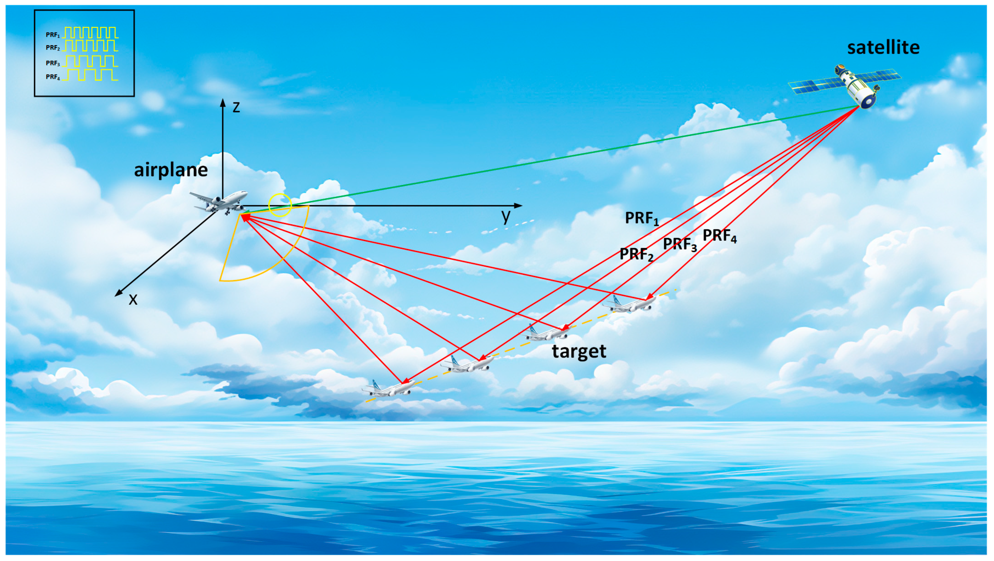
With the iterative upgrades of aerial platforms, early warning detection of airborne targets has become increasingly important. As shown in Figure 1, the TD-MPMF bistatic radar system comprises two main components: the transmitter and the dual-channel receiver. In Figure 1, the TD-MPMF bistatic radar system uses a ground-based radar as the transmitter and an airborne platform as the receiver. However, this bistatic configuration is not limited to those platforms—ground stations, airborne platforms, satellite platforms, or even novel airship platforms can serve as either transmitter or receiver. The ${PRF}_l(l=1,2,\dots ,L)$ are employed periodically in an alternating fashion. The whole cycle spans from ${PRF}_1$ to ${PRF}_L$, covering a total of L different PRFs. Unlike a traditional monostatic radar, the TD-MPMF bistatic radar receiving platform has two receive channels: one channel receives the direct-path signal from the radiation source, while the other channel receives the target-reflected echo signal. The antenna for receiving the direct-path signal is an omnidirectional antenna.

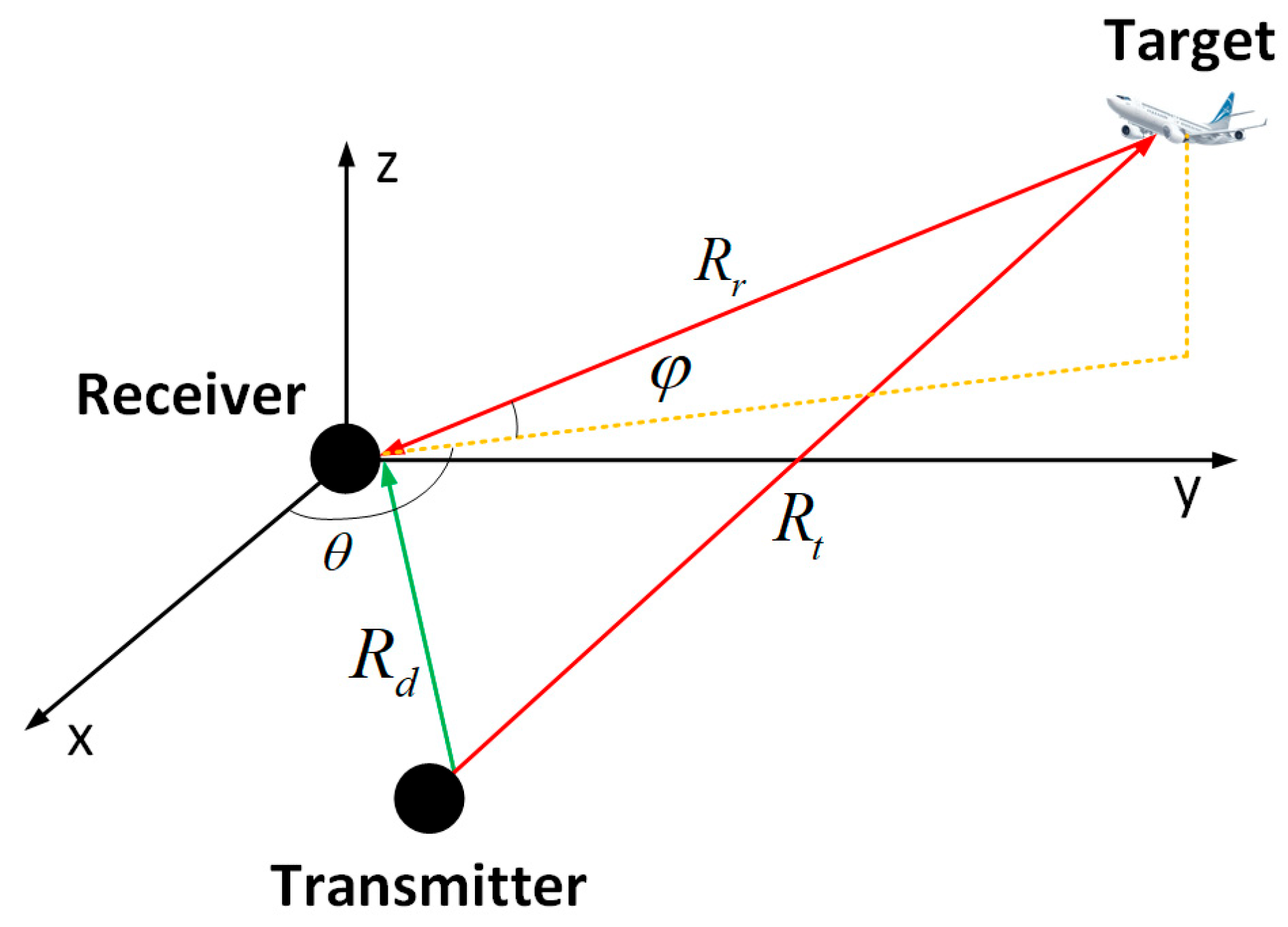
We set the receiving platform as the coordinate origin to establish an $x–y–z$ coordinate system. The geometric relationship among the radiation source, the receiving platform, and the target is shown in Figure 2. Within one coherent processing interval (CPI), the radiation source, target, and receiving platform are assumed to remain relatively stationary under a “stop-and-go” model. $\theta$ is the azimuth angle of the target, and $\phi$ is the elevation angle of the target.

In the TD-MPMF bistatic radar system, range ambiguity typically refers to ambiguity in the two-way range difference. It is the sum of the transmitter-to-target distance and the target-to-receiver distance minus the transmitter-to-receiver distance, expressed as follows:

$$R^{\ast }=R_t+R_r-R_d$$

(1)

where $R_t$ is the distance between the transmitter and the target, $R_r$ is the distance between the target and the receiving platform, and $R_d$ is the distance between the transmitter and the receiving platform. Let $f_l^p$ be the value of the $l$-th PRF, $T_l^p$ is the corresponding pulse repetition interval, $c$ is the speed of light, and $\lambda$ is the wavelength. The maximum unambiguous range is $R_{ul}=c·T_l^p$ and the maximum unambiguous velocity is $V_{ul}=\lambda ·f_l^p/2$.

Assume the radiation source transmits a narrowband linear frequency modulation (LFM) signal; it can be expressed as follows:

$$s_t(\mathit{\tau })=rect({\displaystyle \frac{\tau }{T_p}})exp(j\pi K_r{\tau }^2)$$

(2)

where $rect\left(x\right)=\left\{\begin{array}{c}1,\left|x\right|\le 0.5\\ 0,\left|x\right|\ge 0.5\end{array}\right.$, $T_p$ is the pulse duration, $K_r=B/T_p$ is the frequency modulation ratio, and $B$ is the signal bandwidth.

The transmitted signal reaches the receiving platform through two paths: one path travels a distance of $R_d$ to the reference channel, while the other travels a distance of $R_t+R_r$ to the detection channel. Based on the transmission delays of the two channels, the echo signal can be expressed as follows:

$$\begin{array}{cc}{s}_r\left(\eta ,\tau \right)& =A_r\mathrm{rect}\left[{\displaystyle \frac{\eta }{T_a}}\right]\mathrm{rect}\left[{\displaystyle \frac{\tau -\left(R_t\left(\eta \right)+R_r\left(\eta \right)\right)/c}{T_p}}\right]\hfill \\ & ·\exp \left\{-j\pi K_r{\left(\tau -{\displaystyle \frac{R_t\left(\eta \right)+R_r\left(\eta \right)}{c}}\right)}^2\right\}\hfill \\ & ·\exp \left\{-j2\pi {\displaystyle \frac{R_t\left(\eta \right)+R_r\left(\eta \right)}{\lambda }}\right\}\hfill \end{array}$$

(3)

$$\begin{array}{cc}{s}_d\left(\eta ,\tau \right)& =A_d\mathrm{rect}\left[{\displaystyle \frac{\eta }{T_a}}\right]\mathrm{rect}\left[{\displaystyle \frac{\tau -R_d\left(\eta \right)/c}{T_p}}\right]\hfill \\ & ·\exp \left\{-j\pi K_r{\left(\tau -{\displaystyle \frac{R_d\left(\eta \right)}{c}}\right)}^2\right\}·\exp \left\{-j2\pi {\displaystyle \frac{R_d\left(\eta \right)}{\lambda }}\right\}\hfill \end{array}$$

(4)

where $\tau$ is the fast time, $\eta$ is the slow time, $T_a$ is the coherent integration time, $A_r$ is the amplitude of the target-reflected echo signal, and $A_d$ is the amplitude of the direct-path signal. The Taylor expansion of the two-way range difference can be approximately expressed as follows:

$$R^{*}\left(\eta \right)=R_t\left(\eta \right)+R_r\left(\eta \right)-R_d\left(\eta \right)\approx R_0-\lambda f_d\eta$$

(5)

where $R_t\left(\eta \right)$ is the distance between the transmitter and the target at time $\eta$, $R_r\left(\eta \right)$ is the distance between the receiving platform and the target at time $\eta$, $R_d\left(\eta \right)$ is the distance between the transmitter and the receiving platform at time $\eta$, and $f_d$ is the Doppler frequency.

2.2. Target Model

Assume the target moves in a straight line at a CV (see the proof in Appendix A) in a 3D coordinate system, and the number of targets is unknown and denoted by $m(m=1,2,\dots ,M)$; the number of observation frames is denoted by $k(k=1,2,\dots ,K)$. During the observation period, targets may enter or leave the observation area. The state vector of a target in polar coordinates can be expressed as follows:

$$P_k^m={[R_k^m,v_k^m,{\theta }_k^m,{\phi }_k^m]}^{{\rm T}}$$

(6)

where $R_k^m$ is the radial distance of the target, $v_k^m$ is its radial velocity, ${\theta }_k^m$ is its azimuth angle, ${\phi }_k^m$ is its elevation angle, and $T$ represents matrix transpose.

The transformation between polar coordinates and Cartesian coordinates can be expressed as follows:

$$\left\{\begin{array}{c}{x}_k^m=R_k^m\cos {\phi }_k^m\cos {\theta }_k^m\\ {\dot{x}}_k^m=v_k^m\cos {\phi }_k^m\cos {\theta }_k^m\\ y_k^m=R_k^m\cos {\phi }_k^m\sin {\theta }_k^m\\ {\dot{y}}_k^m=v_k^m\cos {\phi }_k^m\sin {\theta }_k^m\\ z_k^m=R_k^m\sin {\phi }_k^m\\ {\dot{z}}_k^m=v_k^m\sin {\phi }_k^m\end{array}\right.$$

(7)

According to the above relationship, the state vector of the target in the Cartesian coordinate system can be expressed as follows:

$$X_k^m={\left[x_k^m,{\dot{x}}_k^m,y_k^m,{\dot{y}}_k^m,z_k^m,{\dot{z}}_k^m\right]}^{{\rm T}}$$

(8)

where $x_k^m$, $y_k^m$, $z_k^m$ are the position parameters of the target, ${\dot{x}}_k^m$, ${\dot{y}}_k^m$, ${\dot{z}}_k^m$ are their velocity. The state equation of a CV linear motion target is the following:

$$X_{k+1}^m=F{X}_k^m+\mathsf{\Gamma }{U}_k^m$$

(9)

where $U_k^m$ is the random disturbance generated during the target’s motion, modeled as a Gaussian random process with a mean of 0 and a variance of ${\omega }_k^m$. $F$ is the state transition matrix. $\mathsf{\Gamma }$ is the process noise driving matrix.

$$F=\left[\begin{array}{cccccc}1& T_a& 0& 0& 0& 0\\ 0& 1& 0& 0& 0& 0\\ 0& 0& 1& T_a& 0& 0\\ 0& 0& 0& 1& 0& 0\\ 0& 0& 0& 0& 1& T_a\\ 0& 0& 0& 0& 0& 1\end{array}\right]$$

(10)

$$\mathsf{\Gamma }=\left[\begin{array}{ccc}{T}_a^2/2& 0& 0\\ T_a& 0& 0\\ 0& T_a^2/2& 0\\ 0& T_a& 0\\ 0& 0& T_a^2/2\\ 0& 0& T_a\end{array}\right]$$

(11)

The state vector of multiple targets at the $k$-th frame is defined as $P_k={\left[{\left(P_k^1\right)}^{⊺},{\left(P_k^2\right)}^{⊺},\dots ,{\left(P_k^M\right)}^{⊺}\right]}^{⊺}$. The state vector of the m-th target from the 1st frame to the $K$-th frame is defined as $P_{1:K}^m=\left[P_1^m,P_2^m,\dots ,P_K^m\right]$, while that of multiple targets from the 1st frame to the $K$-th frame is defined as $P_{1:K}=\left[P_{1:K}^1,P_{1:K}^2,\dots ,P_{1:K}^M\right]$. In the Cartesian coordinate system, the corresponding state vector can be expressed as $X_k={\left[{\left(X_k^1\right)}^{⊺},{\left(X_k^2\right)}^{⊺},\dots ,{\left(X_k^M\right)}^{⊺}\right]}^{⊺}$, $X_{1:K}^m=\left[X_1^m,X_2^m,\dots ,X_K^m\right]$, and $X_{1:K}=\left[X_{1:K}^1,X_{1:K}^2,\dots ,X_{1:K}^M\right]$.

2.3. Measurement Model

Under the TD-MPMF system, the relationship between the measured ambiguous value ${\widehat{r}}_k^m$ of the target slant range and the true state value $R_k^m$ can be expressed as follows:

$$\left\{\begin{array}{c}{R}_k^m={\widehat{r}}_k^m+i_r\times R_{u1}\\ R_{k+1}^m={\widehat{r}}_{k+1}^m+i_r\times R_{u2}\\ \dots \\ R_{k+L-1}^m={\widehat{r}}_{k+L-1}^m+i_r\times R_{uL}\end{array}\right.$$

(12)

where $i_r$ is the possible ambiguity number of the slant range, $u_r$ is the maximum possible ambiguity number of the slant range, $i_r=0,1,\dots u_r$. Similarly, the relationship between the measured ambiguous value ${\widehat{v}}_k^m$ of the target’s radial velocity and the true state value $v_k^m$ can be expressed as follows:

$$\left\{\begin{array}{c}{v}_k^m={\widehat{v}}_k^m+i_v\times V_{u1}\\ v_{k+1}^m={\widehat{v}}_{k+1}^m+i_v\times V_{u2}\\ \dots \\ v_{k+L-1}^m={\widehat{v}}_{k+L-1}^m+i_v\times V_{uL}\end{array}\right.$$

(13)

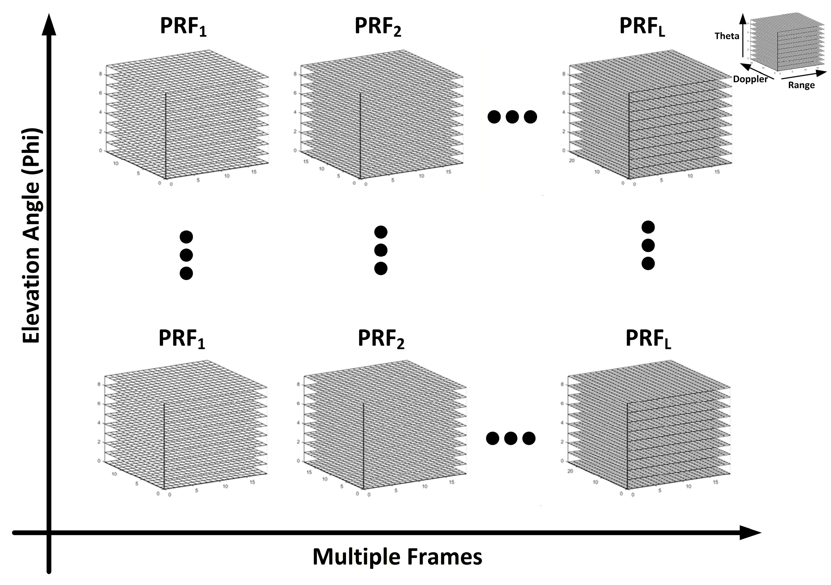
where $i_v$ is the possible ambiguity number of the radial velocity, and $u_v$ is the maximum possible ambiguity number of the radial velocity, $i_v=0,1,\dots u_v$. Assume the signal’s center frequency is $f_c=c/\lambda$, and the signal’s sampling rate is $f_s$. The range resolution is ${\rho }_r=c/B$. The Doppler resolution is ${\rho }_d=1/T_a$ and the corresponding velocity resolution is ${\rho }_v={\rho }_d·\lambda$. The resolutions of azimuth and elevation angles are ${\rho }_{\theta }$ and ${\rho }_{\phi }$, respectively. These are related to the 3dB beamwidths of the antenna in the azimuth and elevation directions, respectively [17]. After CFAR detection of the echo data, discrete measurement data is obtained. The measurement data is a four-dimensional data block as shown in Figure 3, and for the $k$-th frame it can be expressed as follows:

$$\begin{array}{l}\left\{{\tilde{z}}_k^l\left(i,j,p,q\right),i=1,2,\dots ,N_r^l,j=1,2,\dots ,N_d^l\right.,\\ \left.p=1,2,\dots ,N_{\theta }^l,q=1,2,\dots ,N_{\phi }^l\right\}\end{array}$$

(14)

where ${\tilde{z}}_k^l\left(i,j,p,q\right)$ is the amplitude corresponding to the $l$-th PRF unit of the $k$-th frame, $N_r^l=⌈R_{ul}/{\rho }_r⌉$, $N_d^l=⌈V_{ul}/{\rho }_d⌉+1$, $N_{\theta }^l=⌈\mathsf{\Theta }/{\rho }_{\theta }⌉$, $N_{\phi }^l=⌈\mathsf{\Phi }/{\rho }_{\phi }⌉$, and $⌈·⌉$ represents the rounding up operation. In the TD-MPMF system, the relationship between $k$ and $l$ can be expressed as follows:

$$l=\left(k-1\right)\mathrm{mod}L+1$$

(15)

where mod is the modulo operator.

3. Proposed Robust TD-MPMF-SVM Algorithm

3.1. TD-MPMF Framework

Due to its bistatic configuration in the TD-MPMF system, the echoes inevitably contain direct waves and other types of clutter (multipath echoes, stationary clutter). Therefore, preprocessing of the echo data is necessary, which mainly includes two parts: direct wave suppression [18,19,20] and clutter suppression [21,22].

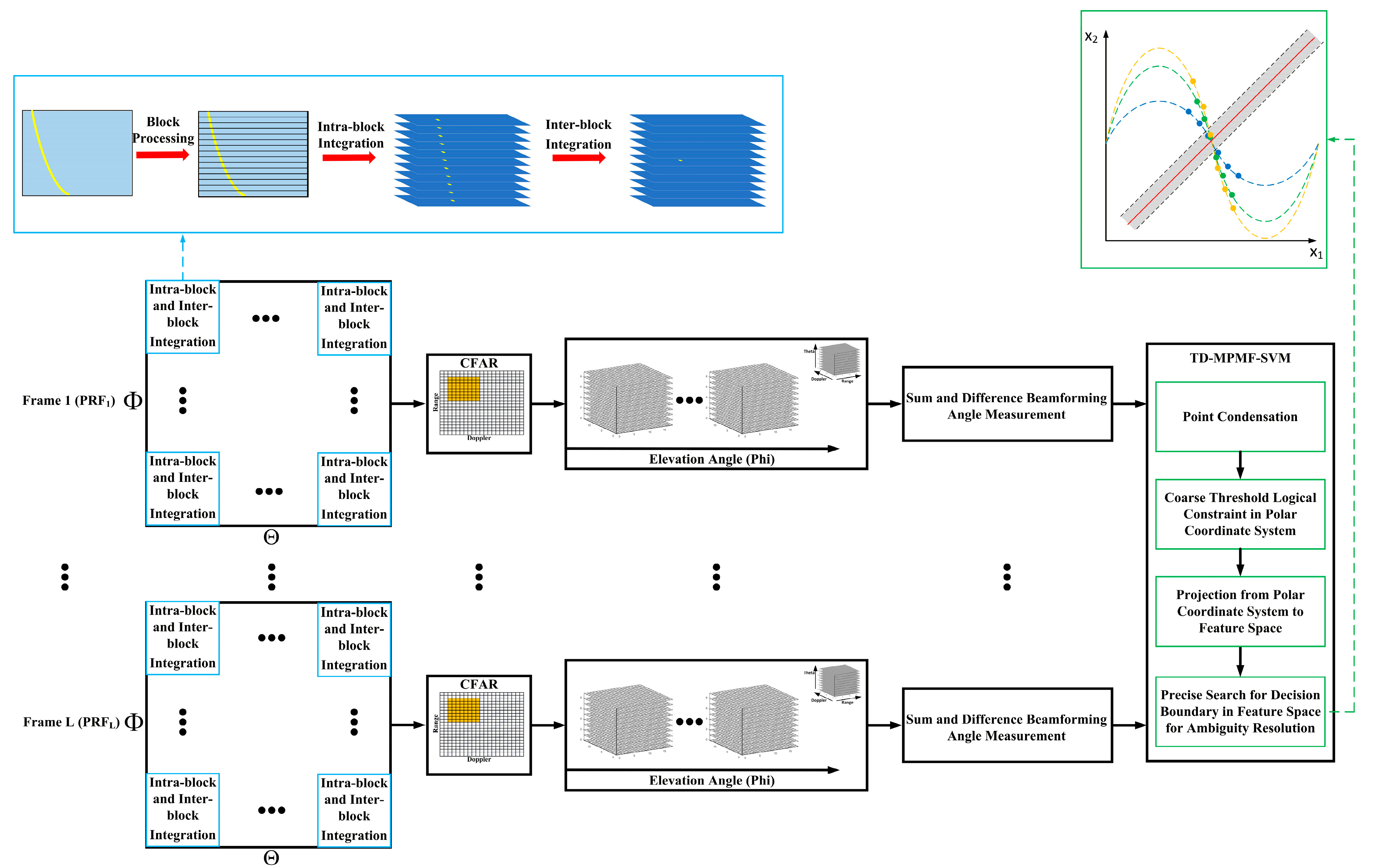
After performing data preprocessing on the echo data, the TD-MPMF method is applied. The processing flow-chart of the TD-MPMF method is shown in Figure 4. After preprocessing, the echo signal $s_r\left(\eta ,\tau \right)$ is transformed into the range frequency domain by performing FFT along the range dimension, which can be expressed as follows:

$$\begin{array}{c}{s}_r\left(\eta ,f_{\tau }\right)=A_m\mathrm{rect}\left[{\displaystyle \frac{\eta }{T_a}}\right]\mathrm{rect}\left[f_{\tau }\right]·\exp \left\{j\pi {\displaystyle \frac{{f_{\tau }}^2}{K_r}}\right\}\\ ·\exp \left\{-j2\pi {\displaystyle \frac{f_{\tau }+f_c}{c}}\left(R_t\left(\eta \right)+R_r\left(\eta \right)\right)\right\}\end{array}$$

(16)

where $f_{\tau }$ is the range–frequency domain. The compensation of the range quadratic phase factor in the range–frequency domain can be expressed as follows:

$$H\left(f_{\tau }\right)=\exp \left\{-j\pi {\displaystyle \frac{{f_{\tau }}^2}{K_r}}\right\}$$

(17)

Next, coherent processing is performed by segmenting the echo signal into sub-blocks. The criterion for segmentation is that within each sub-block, the target’s range migration (RM) and Doppler migration (DM) can be ignored. The echo signal is segmented in the azimuth dimension, and the segmentation must satisfy the following conditions:

$$\lambda f_d{t}_{sub}\le {\displaystyle \frac{c}{fs}}\Rightarrow t_{sub}\le {\displaystyle \frac{c}{\lambda f_{d}fs}}$$

(18)

where $t_{sub}$ is the coherent integration time for each sub-block after segmentation. For the segmented sub-block data, the effects of RM and DM can be ignored, allowing for a direct azimuth FFT on the sub-block data. This results in coherent processing in the azimuth direction for the echo signal.

After the first stage of coherent processing, the echo signal undergoes coherent integration within each sub-block. However, relative RM and Doppler phase deviation still exist between the sub-blocks, meaning that direct coherent integration cannot be performed. The relative RM and Doppler phase deviation between the sub-blocks must be compensated. After the intra-block coherent processing, the echo signal is accumulated in the azimuth direction in the 2D frequency domain. The processed echo signal can be expressed as follows:

$$s_{nsub}\left(f_{d\_temp},f_{\tau }\right)=A_{m}P\left(f_{\tau }\right)\times \exp \left(-j2\pi {\displaystyle \frac{f_{\tau }+f_c}{c}}R\left(f_{d\_temp}\right)\right)$$

(19)

$$s_r=\left[\begin{array}{c}{s}_{1sub}\\ s_{2sub}\\ ⋮\\ s_{N^{*}sub}\end{array}\right]$$

(20)

where $f_{d\_temp}$ is the Doppler bin where the target is located, $s_{nsub}$ is the $n$-th sub-block of the echo signal, $n=1,2,\dots ,N^{*}$, and $P\left(·\right)$ is the signal after performing FFT on the range dimension. The different positions reflect the Doppler frequency of the target, which indicates the relative position offset of each sub-block at that frequency location. To reduce the relative RM between sub-block data, the relative RM factor can be compensated for in the range frequency domain, aligning the same target from different sub-block data to the same range bin. The relative RM compensation factor between sub-blocks can be expressed as follows:

$$H_{rc}=\exp \left\{{\displaystyle \frac{-j2\pi \left(f_c+f_{\tau }\right)}{c}}\lambda f_{d\_temp}{k}^{*}{T}_b\right\}$$

(21)

where $T_b$ is the time duration of the sub-block data, and $k^{*}$ is the relative offset (in terms of the number of sub-blocks) between sub-blocks. By performing the inverse fast fourier transform (IFFT) along the range dimension on the inter-block coherent parameter space matrix, and converting it to the moving target parameter domain, the final parameter matrix can be expressed as follows:

$$Spara\left(R_0,fd\right)=rIFFT\left({\displaystyle \sum _{n=1}^{N^{*}}{S}_{nsub}·H_{rc}}\right)$$

(22)

The inter-block coherent result is subjected to CFAR detection [23], resulting in discrete measurement data ${\tilde{z}}_k^l\left(i,j,p,q\right)$. Next, the received measurement data from the antenna array undergoes sum-and-difference beamforming for angle estimation [24,25,26], resulting in the azimuth and elevation angles of all detected targets. Then, the angle-estimated measurement data is input into the ambiguity resolution module. The relevant algorithms for this part will be discussed in detail in the next section. Finally, the ambiguity resolution results are tracked using Kalman filtering, and the target trajectory is then obtained [27,28,29].

3.2. TD-MPMF-SVM Algorithm

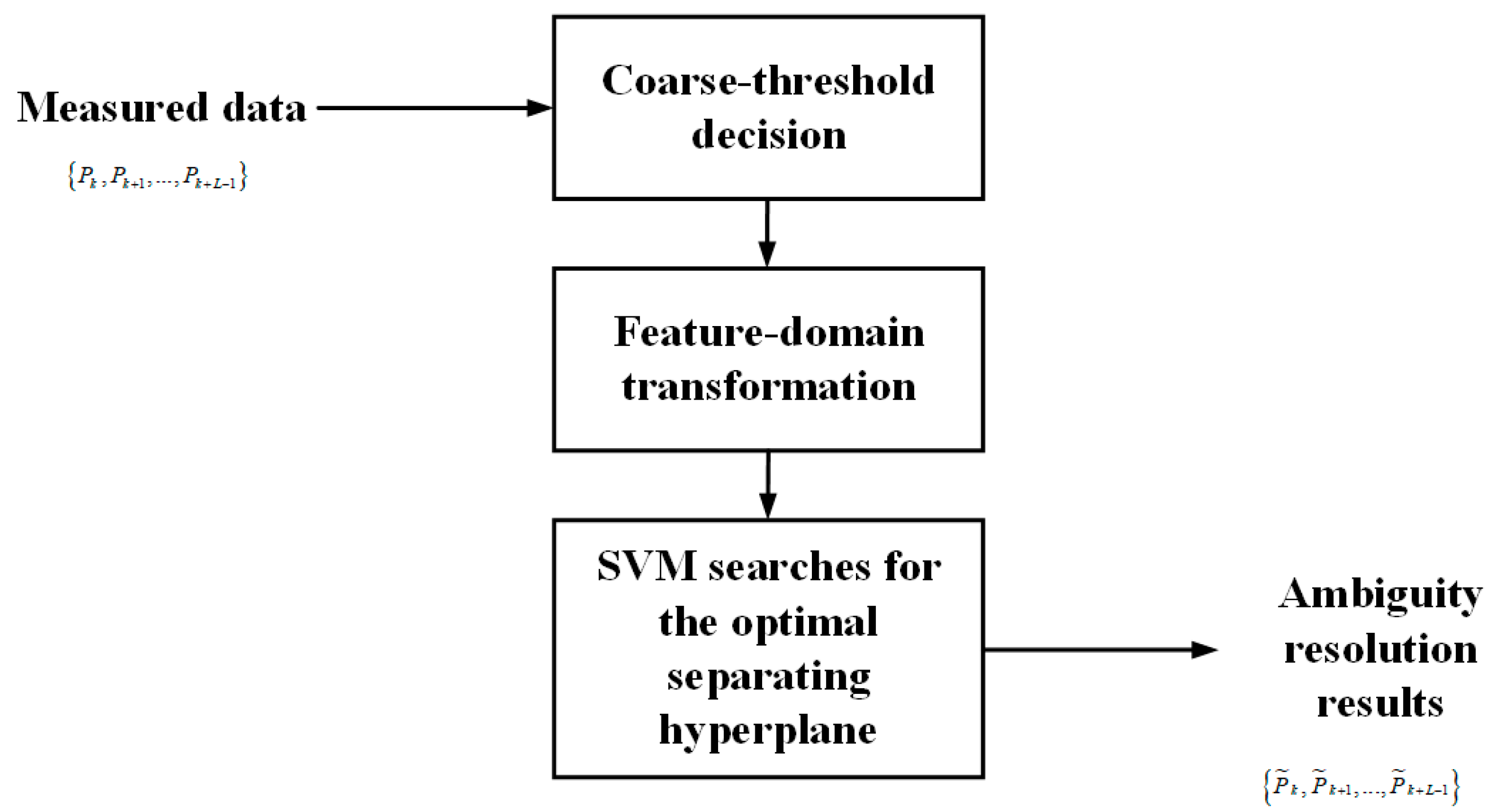
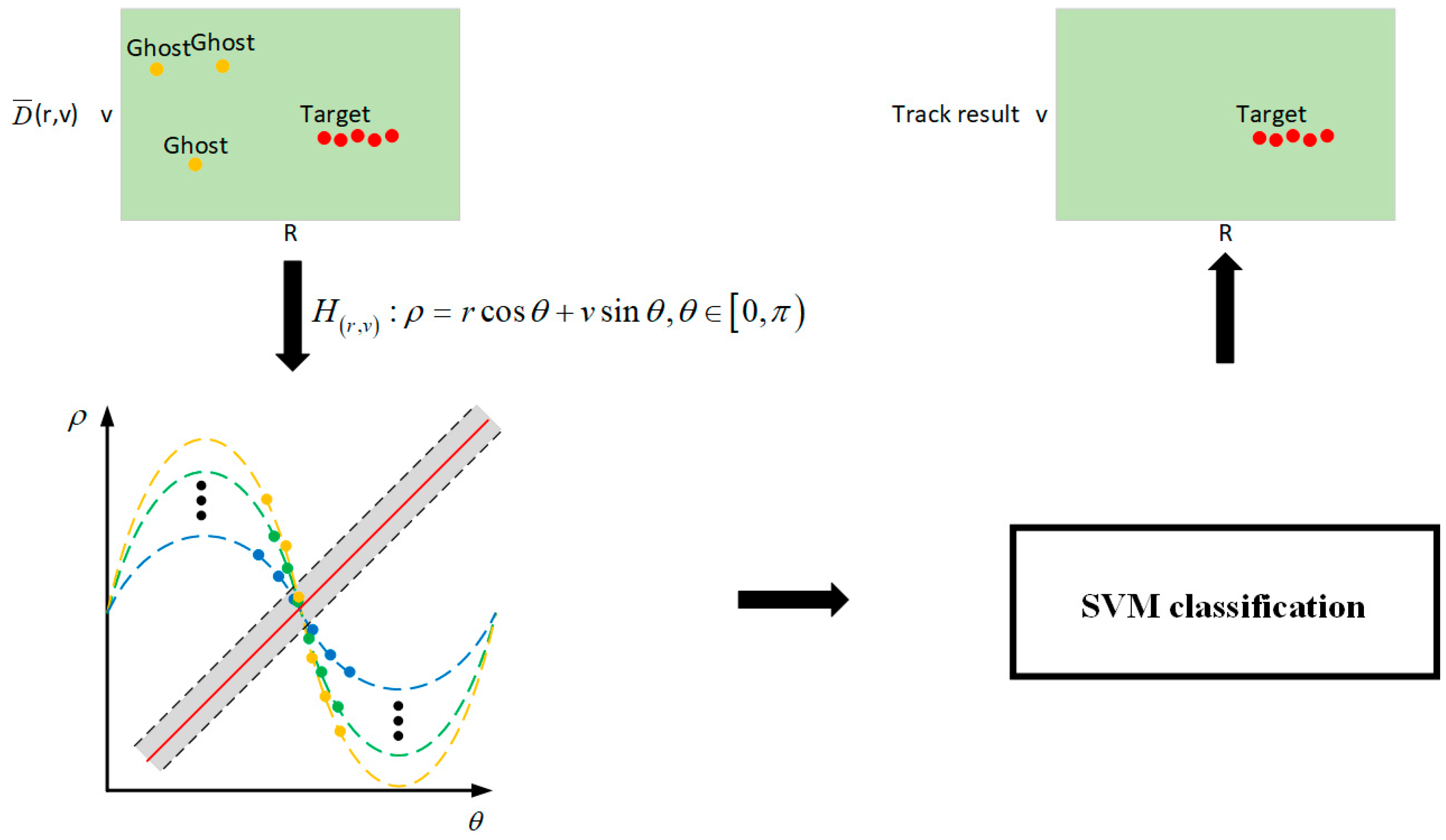
After algorithm processing in the previous section, the azimuth and elevation angles for all the measurement data have been obtained. For convenience in the following discussion, the set of all measurement data is denoted as $P_k$ and the ambiguity resolution result is denoted as ${\tilde{P}}_k$. The TD-MPMF-SVM algorithm takes discrete measurements obtained under multi-PRF as its input and its output is the target’s true range and velocity after ambiguity resolution. This algorithm divides the coherent integration time of a single frame into L subframes according to the number of PRFs. By leveraging the coupling relationship between multi-PRF, the ambiguity in target sequence measurements is resolved in three steps. The first step is that potential track points are filtered using a coarse threshold. The second step is that the data is converted from polar coordinates to the feature domain through a feature-domain transformation. The third step is that an SVM identifies the optimal hyperplane to produce the ambiguity resolution results. The block diagram of the ambiguity resolution algorithm is shown in Figure 5.

1.

The multi-frame multi-PRF measurement data extension involves setting a coarse threshold and using a logical method to evaluate the inter-frame matrix, thus filtering potential target tracks;

The measurement data matrix for the $k$-th frame with $L$ PRFs is denoted as $\left\{{\tilde{z}}_k^1,{\tilde{z}}_k^2,\dots ,{\tilde{z}}_k^L\right\}$. To construct the state matrix for all detected measurement data based on the maximum unambiguous range $R_{ul}$ and maximum unambiguous velocity $V_{ul}$, we assume that a certain target’s measurement value is $P_k^m$. The corresponding state matrix can be expressed as follows:

$$\left[\begin{array}{ccc}[r_k^m,v_k^m]& \dots & [r_k^m,v_k^m+N_v·V_{ul}]\\ \dots & \dots & \dots \\ [r_k^m+N_r·R_{ul},v_k^m]& \dots & [r_k^m+N_r·R_{ul},v_k^m+N_v·V_{ul}]\end{array}\right]$$

(23)

where $N_r$ is the maximum possible range ambiguity number, and $N_v$ is the maximum possible velocity ambiguity number. In the polar coordinate system, the matrix $P_k$ can be extended ${\overline{P}}_k$ using Equation (23), and the collection of $L$ PRFs measurement data can be expressed as follows:

$${\overline{P}}_{k:k+L-1}=\left\{\left.{\overline{P}}_k,{\overline{P}}_{k+1},\dots ,{\overline{P}}_{k+L-1}\right|\left(r,v\right)\right\}$$

(24)

Select two adjacent matrices from the set ${\overline{P}}_{k:k+L-1}$ and calculate their relative velocity difference and acceleration:

$${\displaystyle \frac{r_{k+i+1}^{m_{k+i+1}}-r_{k+i}^{m_{k+i}}}{T_a}}-v_{k+i}^{m_{k+i}}=\Delta {\overline{v}}_{k+i},i=0,1,\dots ,L-2$$

(25)

$${\displaystyle \frac{v_{k+i+1}^{m_{k+i+1}}-v_{k+i}^{m_{k+i}}}{T_a}}={\overline{a}}_{k+i},i=0,1,\dots ,L-2$$

(26)

The collection of all the relative velocity differences and accelerations for all PRFs can be represented as follows:

$$\Delta {\overline{v}}_{L-1}=\left\{\Delta {\overline{v}}_k,\Delta {\overline{v}}_{k+1},\dots ,\Delta {\overline{v}}_{k+L-2}\right\}$$

(27)

$${\overline{a}}_{L-1}=\left\{{\overline{a}}_k,{\overline{a}}_{k+1},\dots ,{\overline{a}}_{k+L-2}\right\}$$

(28)

$∆{\overline{v}}_{L-1}$ and ${\overline{a}}_{L-1}$ should both satisfy the following condition:

$$\left\{\begin{array}{c}\Delta {\overline{v}}_{\min }\le \max \left\{\left|\Delta {\overline{v}}_{L-1}\right|\right\}\le \Delta {\overline{v}}_{\max }\\ {\overline{a}}_{\min }\le \max \left\{\left|{\overline{a}}_{L-1}\right|\right\}\le {\overline{a}}_{\max }\end{array}\right.$$

(29)

where $∆{\overline{v}}_{min}$ and $∆{\overline{v}}_{max}$ are the velocity threshold set based on prior knowledge, and ${\overline{a}}_{min}$ and ${\overline{a}}_{max}$ are the acceleration threshold set based on prior knowledge. Examine the measurement values of the set ${\overline{P}}_{k:k+L-1}$ by exhaustive search, and if they satisfy Equation (29), store them in set $D\left(r,v\right)$.

2.

Perform point condensation on the filtered track set, select stationary and low-speed targets, and then perform a coordinate transformation to convert them from polar coordinates to feature space. Use SVM for classification to find the separating hyperplane, thereby obtaining the target ambiguity resolution result.

After coarse thresholding, the potential target track set $D\left(r,v\right)$ is obtained, where each track is represented by $L:\left\{\left(r_1,v_1\right),\left(r_2,v_2\right),\dots ,\left(r_L,v_L\right)\right\}$.

Point condensation is performed on the track $L$ to filter out stationary and low-speed targets. The track for stationary targets is represented by $L_{static}:\left\{\left(r,0\right),\left(r,0\right),\dots ,\left(r,0\right)\right\}$. For low-speed targets, the distance relationship between frames can be expressed as follows:

$$\left\{\begin{array}{c}{r}_2=r_1+v_1·T_a\\ r_3=r_2+v_2·T_a\\ \dots \\ r_L=r_{L-1}+v_{L-1}·T_a\end{array}\right.$$

(30)

Since it is a low-speed target, the condition is satisfied when

$${\displaystyle \sum _{i=1}^{L-1}{v}_i{T}_a}\le 3·{\rho }_r$$

(31)

It can be assumed that $r_1=r_2=\cdots =r_L$. The point condensation pseudo-code is presented in

Table 1. TD-MPMF-SVM point condensation pseudo-code.

Note: Point set $D\left(r,v\right)$, point track set $L:\left\{\left(r_1,v_1\right),\left(r_2,v_2\right),\dots ,\left(r_L,v_L\right)\right\}$, maximum range value $∆r_{max}$, maximum velocity value $∆v_{max}$.
1	Input: $D$, $L$, $∆r_{max}$, $∆v_{max}$;
2	Output: $L^{*}$;
3	$r_{min}=min\left(\left\{r_1,r_2,\dots ,r_L\right\}\right)$, $r_{max}=max\left(\left\{r_1,r_2,\dots ,r_L\right\}\right)$;
4	$v_{min}=min\left(\left\{v_1,v_2,\dots ,v_L\right\}\right)$, $v_{max}=max\left(\left\{v_1,v_2,\dots ,v_L\right\}\right)$;
5	$∆r=r_{max}-r_{min}$, $∆v=v_{max}-v_{min}$;
6	If$∆r\le ∆r_{max}$ and $∆v\le ∆v_{max}$ then
7	$L^{*}=L$
8	delete $L$ in $D\left(r,v\right)$
9	End if

.

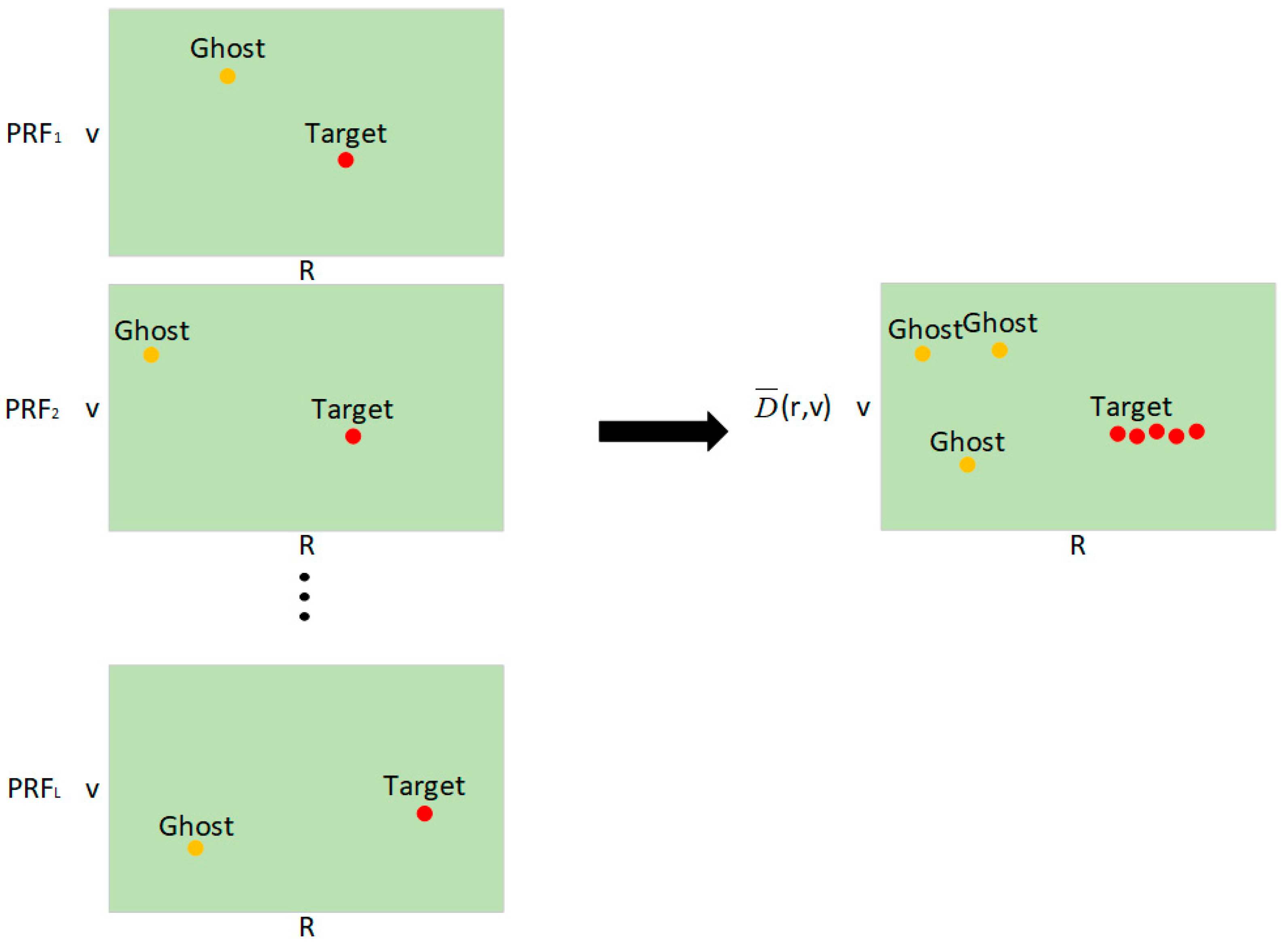
After removing stationary and low-speed clutter, the remaining measurements $\overline{D}\left(r,v\right)$ are used for tracking. In a TD-MPMF system, targets exhibit range shifts across different PRFs. However, because the targets move at CV, the same target maintains a linear (or approximately linear) relationship across the multi-PRF measurements, as illustrated in Figure 6.

Transform the remaining track set $\overline{D}\left(r,v\right)$ from polar coordinates to the feature space; it can be represented as follows:

$$H_{\left(r,v\right)}:\rho =r\cos \theta +v\sin \theta ,\theta \in \left[0,\pi \right)$$

(32)

Therefore, for each measurement point in the track set $\overline{D}\left(r,v\right)$, a curve can be obtained. For the same target in the CV mode, the $L$ curves must intersect at $\left(v,{\displaystyle \frac{\pi }{2}}\right)$ (see the proof in Appendix B). The SVM-based fine-stage procedure is shown in Figure 7.

For a CV target, the positive class voting points from the target are located at or clustered around the intersection $\left({\rho }^{*},{\theta }^{*}\right)=\left(v,{\displaystyle \frac{\pi }{2}}\right)$. Therefore, the ideal classification hyperplane should satisfy the following:

1.

For positive class points, it is required that ${\omega }^{T}x+b$ approaches 0 at the intersection point;

2.

For negative class points, their values should have a sufficient gap from the positive class to ensure correct classification.

Specifically, since the intersection point is within the positive class, it must satisfy the following:

$${\omega }^T\left(\begin{array}{c}v\\ {\displaystyle \frac{\pi }{2}}\end{array}\right)+b=0$$

(33)

This provides a geometric constraint for the hyperplane solved by the SVM. Only when all positive class points exhibit consistency in the $H_{\left(r,v\right)}$ space can the SVM find a maximum margin-separating hyperplane that effectively divides the positive and negative classes. On the contrary, if the positive class points do not exhibit good linear separability in the $H_{\left(r,v\right)}$ space, the SVM will not be able to find a hyperplane that satisfies the conditions for all support vectors.

4. Simulation and Experimental Results

4.1. Simulation Results

The detection performance of the TD-MPMF-SVM algorithm is compared with that of the MPMF-AM algorithm outlined in [13]. The performance metrics used in the algorithm performance comparison are described as follows:

1.

Optimal sub-pattern assignment (OSPA) distance;

In mathematics, the OSPA distance is used to evaluate the difference between two finite sets in terms of both the number of elements and the individual differences [30,31]. Let $d^{\left(c_{cut}\right)}\left(\overline{x},x\right)≔\mathrm{m}\mathrm{i}\mathrm{n}(c_{cut},‖\widehat{x}-x‖)$, where $c_{cut}$ is the cutoff distance, $X=\left\{x_1,x_2,\dots ,x_m\right\}$ is the target true state vector, while $\widehat{X}=\left\{{\widehat{x}}_1,{\widehat{x}}_2,\dots ,{\widehat{x}}_n\right\}$ is the estimated target state vector. For $p\ge 1$, the OSPA distance is calculated as follows:

$${\overline{d}}_{OSPA,p}^{(c_{cut})}(\widehat{X},X):=\left\{\begin{array}{c}{({\displaystyle \frac{1}{m}}(\underset{\pi \in {\Pi }_m}{\min }{\displaystyle \sum _{i=1}^n{d}^{(c_{cut})}{({\widehat{x}}_i,x_{\pi (i)})}^p+c_{cut}^p(m-n)}))}^{{\displaystyle \frac{1}{p}}},m\ge n>0\\ {\overline{d}}_{OSPA,p}^{(c_{cut})}(X,\widehat{X}),n>m>0\end{array}\right.$$

(34)

If $m=n=0$, ${\overline{d}}_{OSPA,p}^{\left(c_{cut}\right)}\left(X,\widehat{X}\right)={\overline{d}}_{OSPA,p}^{\left(c_{cut}\right)}\left(\widehat{X},X\right)=0$. $p$ is the distance order. In this paper, we set $p=1$ and $c_{cut}=1$.

2.

Target detection probability.

This represents the probability that the estimated state value of the target deviates from the true value within three grid cells.

The simulation scenario is as shown in Figure 1. The number of PRFs in the multiple PRF radar system is set to $L=4$, and the relevant radar system parameters are shown in

Table 2. Multiple PRF radar system parameters.

Parameter	Value	Parameter	Value
$\mathsf{\Theta }$	[−60°~60°]	$\mathsf{\Phi }$	[−60°~60°]
$R$	[0~1000 km]	$V$	$[-600 \mathrm{m}/\mathrm{s}~600 \mathrm{m}/\mathrm{s}$]
$f_s$	2.5 MHz	${\rho }_r$	150 m
${\rho }_v$	$0.24 \mathrm{m}/\mathrm{s}$	${\rho }_{\theta }$	1°
${\rho }_{\phi }$	1°	$f_c$	$1.25 \mathrm{G}\mathrm{H}\mathrm{z}$
$B$	$2 \mathrm{M}\mathrm{H}\mathrm{z}$	$T_p$	$100 \mu \mathrm{s}$
${PRF}_1$	$900 \mathrm{H}\mathrm{z}$	${PRF}_2$	$1200 \mathrm{H}\mathrm{z}$
${PRF}_3$	$1500 \mathrm{H}\mathrm{z}$	${PRF}_4$	$2100 \mathrm{H}\mathrm{z}$

. Since the coherent integration time for all PRFs is 1 s, the corresponding pulse numbers are 900, 1200, 1500, and 2100. In the simulation, the PRF values are set with a wide range, covering low, medium, and high PRF modes. The purpose of this setup is to verify that the TD-MPMF-SVM algorithm is applicable to all PRF modes.

Establish an East-North-Up (ENU) coordinate system with the receiving platform as the origin, where the $x$-axis points east, the $y$-axis points north, and the $z$-axis points upward (towards the sky). The smallest angle required to rotate clockwise or counterclockwise from the north direction around the $z$-axis to the projection of the target point on the $xoy$ plane is denoted as $\theta$. A clockwise rotation is considered positive, and the azimuth angle ranges from −180° to 180°. $\phi$ is defined as the angle between the line connecting the origin and the target point and the $xoy$ plane. The elevation angle is positive when the target is above the $xoy$ plane and negative when it is below the $xoy$ plane, with a range from −90° to 90°. The receiving platform is an aircraft platform, flying in the stratosphere at an altitude of 11,000 m. The initial coordinates of the high-orbit satellite are $\left(-\mathrm{708,000} \mathrm{m}, -\mathrm{2,138,000} \mathrm{m}, \mathrm{36,000,000} \mathrm{m}\right)$. The velocity of the high-orbit satellite is 3000 m/s.

To more effectively demonstrate the performance of the algorithm, a time-varying scenario is designed. The total number of simulation frames is 100, with a maximum of five targets, all with CV linear motion. The appearance times of the five targets are 0 s, 20 s, 40 s, 60 s, and 80 s, respectively. Their initial distance, radial velocity, azimuth angle, and elevation angle are as follows: $\left\{\left[600 \mathrm{k}\mathrm{m},500\mathrm{m}/\mathrm{s},45°,5°\right],\left[600 \mathrm{k}\mathrm{m},425\mathrm{m}/\mathrm{s},30°,-2°\right],\left[700 \mathrm{k}\mathrm{m},133.33\mathrm{m}/\mathrm{s},60°,3°\right],\left[700 \mathrm{k}\mathrm{m},175\mathrm{m}/\mathrm{s},75°,2°\right],\left[800 \mathrm{k}\mathrm{m},60\mathrm{m}/\mathrm{s},15°,-4°\right]\right\}$.

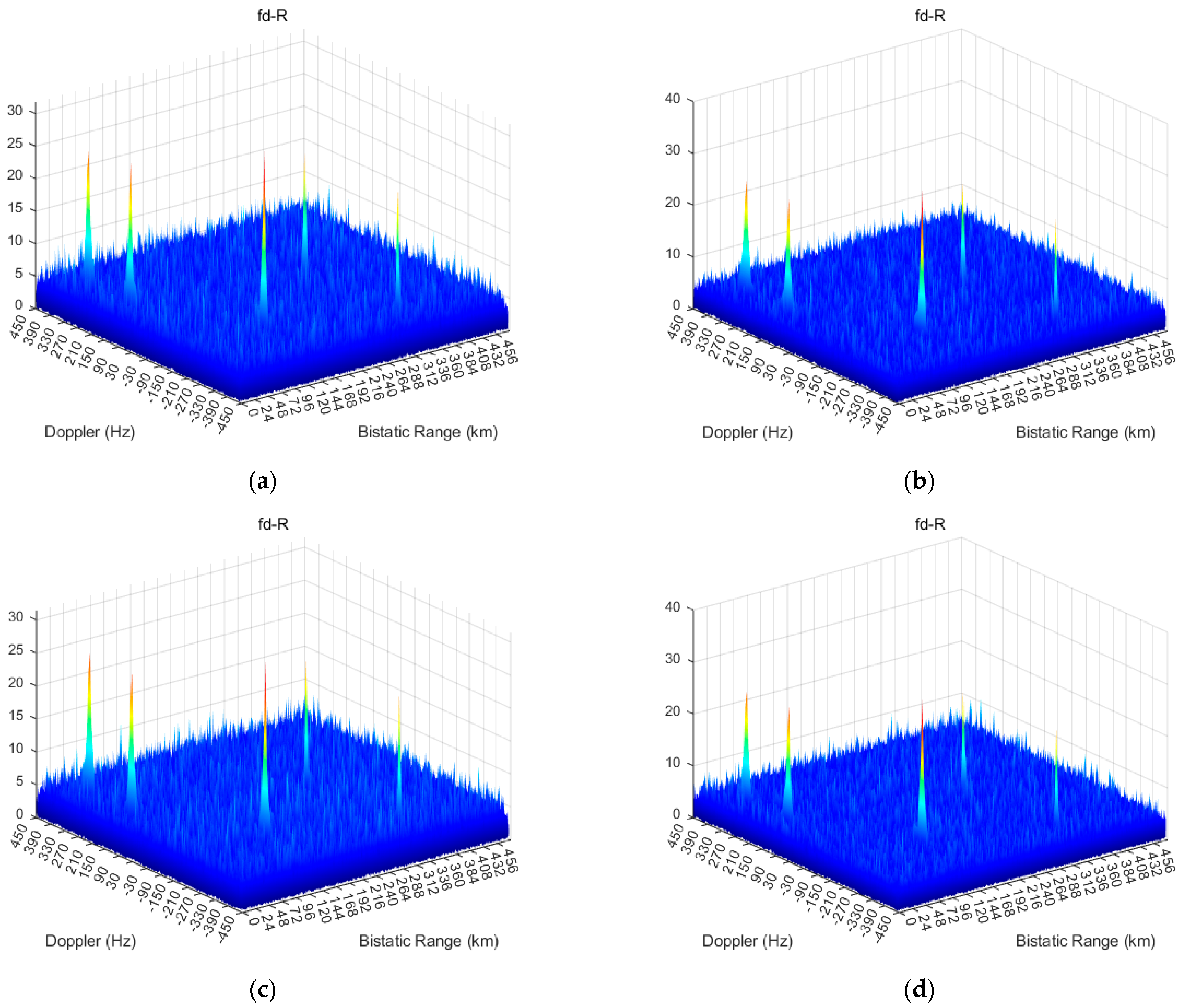
Coherent integration results in the Doppler/range domain for four consecutive frames are presented. All coherent integration results were obtained in the presence of range and Doppler ambiguities. At k = 80, 81, 82, 83, the coherent integration results of the target are shown in Figure 8. The figure shows the coherent integration results for five targets under different PRFs. It can be observed that, under TD PRF mode, the same targets generate relative range.

The CFAR parameters are shown in

Table 3. The parameters of CFAR detection.

Parameter	Value
CFAR type	CA-CFAR
Training cells (per side)	5
Guard cells (per side)	2
False alarm rate	10−6

. We performed CFAR detection on the results of the secondary coherent processing to obtain the target measurements as shown in

Table 4. The Doppler results of target measurements from CFAR detection.

Frame	80	81	82	83
Target	$f_d\left(\mathrm{H}\mathrm{z}\right)$	$f_d\left(\mathrm{H}\mathrm{z}\right)$	$f_d\left(\mathrm{H}\mathrm{z}\right)$	$f_d\left(\mathrm{H}\mathrm{z}\right)$
1	121.2	119.8	121.2	119.8
2	308.8	308.8	308.8	307.4
3	−219	−219	−219	−219
4	14.8	14.8	14.8	13.4
5	−346.4	−346.4	−345	−347.8

and

Table 5. The range results of target measurements from CFAR detection.

Frame	80	81	82	83
Target	$R\left(\mathrm{m}\right)$	$R\left(\mathrm{m}\right)$	$R\left(\mathrm{m}\right)$	$R\left(\mathrm{m}\right)$
1	39,120	39,360	39,480	39,720
2	41,040	41,160	41,280	41,520
3	138,120	138,240	138,240	138,360
4	306,960	307,440	307,800	308,400
5	325,080	325,560	326,160	326,760

.

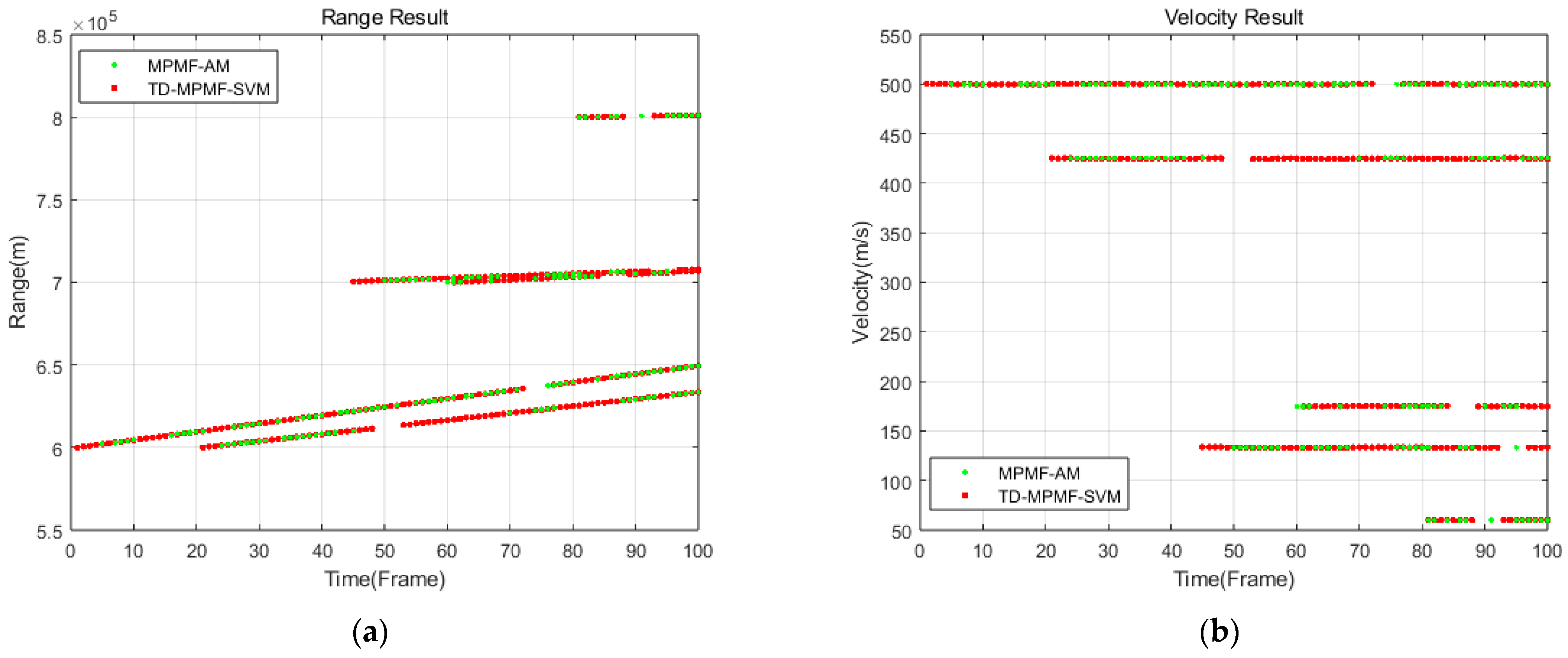
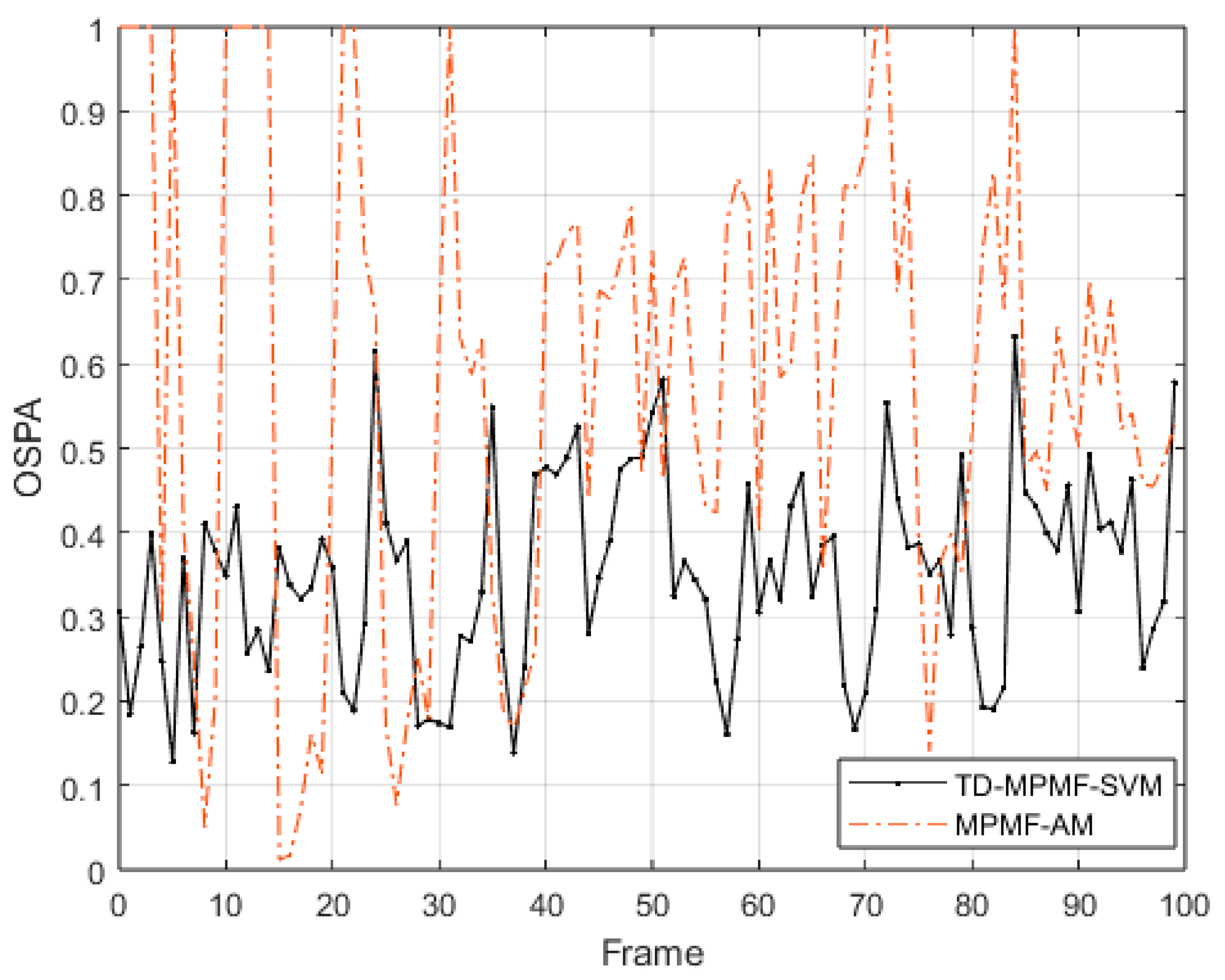
To verify the algorithm’s effectiveness in suppressing ghosts, ghosts are generated at each time step using a random process. The generation process of ghosts follows a Poisson distribution with an intensity of ${\lambda }^{\left(p\right)}$, and their spatial distribution follows a uniform distribution. When ${\lambda }^{\left(p\right)}=20$, the ambiguity resolution results of the two algorithms are shown in Figure 9, and the OSPA distance results are shown in Figure 10. Figure 9 compares the frame-by-frame range and velocity estimates for five targets obtained by the baseline MPMF-AM and the proposed TD-MPMF-SVM algorithm. Figure 9 shows that the MPMF-AM algorithm produces more frequent track fragmentation, while the proposed TD-MPMF-SVM method more accurately and continuously recovers the targets’ true bistatic ranges and radial velocities. Across the full sequence of Figure 10, TD-MPMF-SVM yields systematically lower OSPA values than MPMF-AM, indicating that the proposed method attains smaller combined errors in target localization and target number estimation. The proposed TD-MPMF-SVM algorithm significantly reduces OSPA errors relative to MPMF-AM, indicating improved ambiguity resolution and more continuous target tracking under TD-MPMF mode.

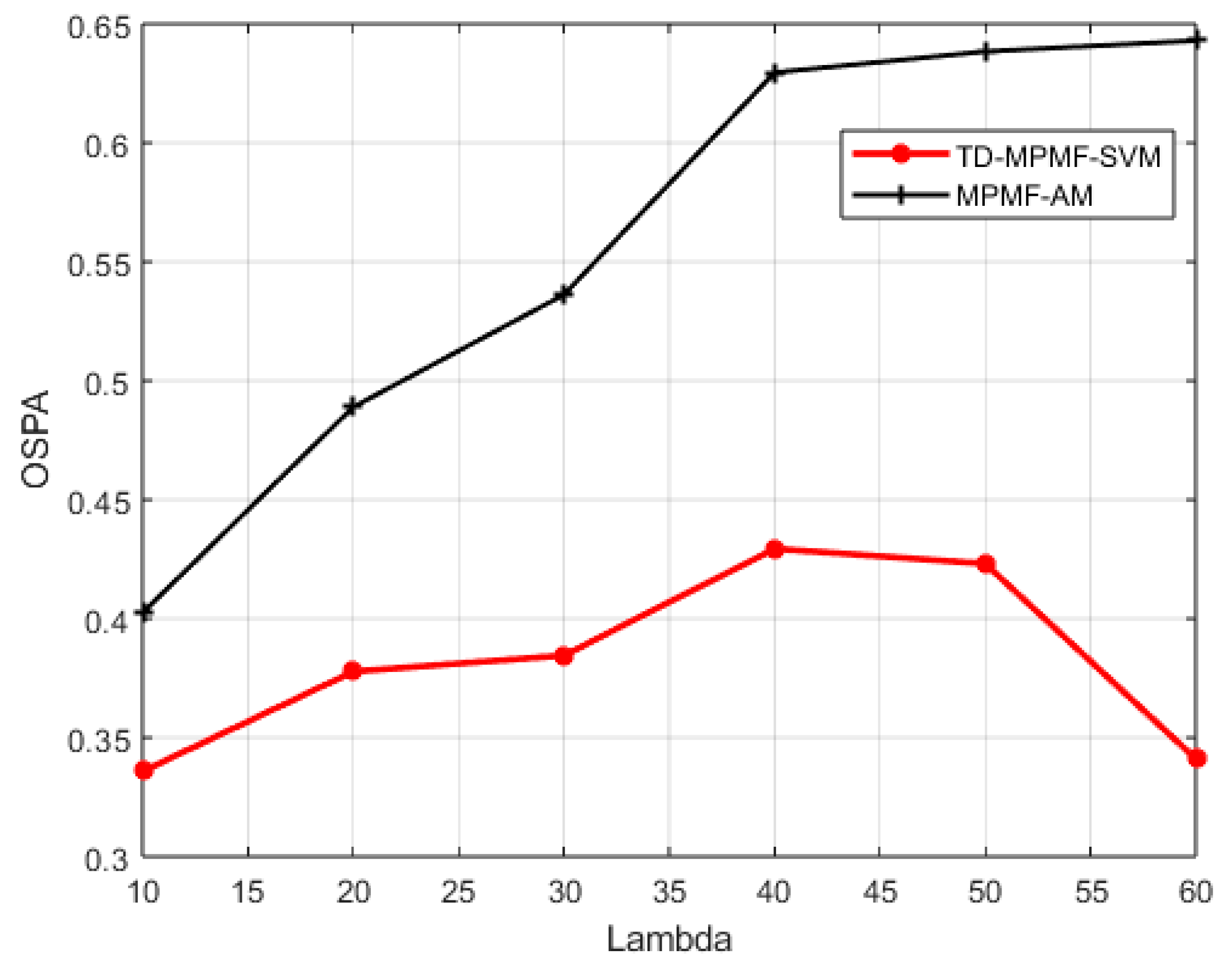
To demonstrate the detection performance of the algorithm under different clutter intensities, a single target $\left[600 \mathrm{k}\mathrm{m},500 \mathrm{m}/\mathrm{s},45°,5°\right]$ is simulated. The intensity of the Poisson random process is set to ${\lambda }^{\left(p\right)}=10, 20, 30, 40, 50, 60,$, and each ${\lambda }^{\left(p\right)}$ is tested with 100 Monte Carlo trials. The average OSPA distances of the two algorithms are shown in Figure 11. The results clearly demonstrate that the proposed TD-MPMF-SVM algorithm achieves better tracking performance than the MPMF-AM algorithm under different clutter intensities.

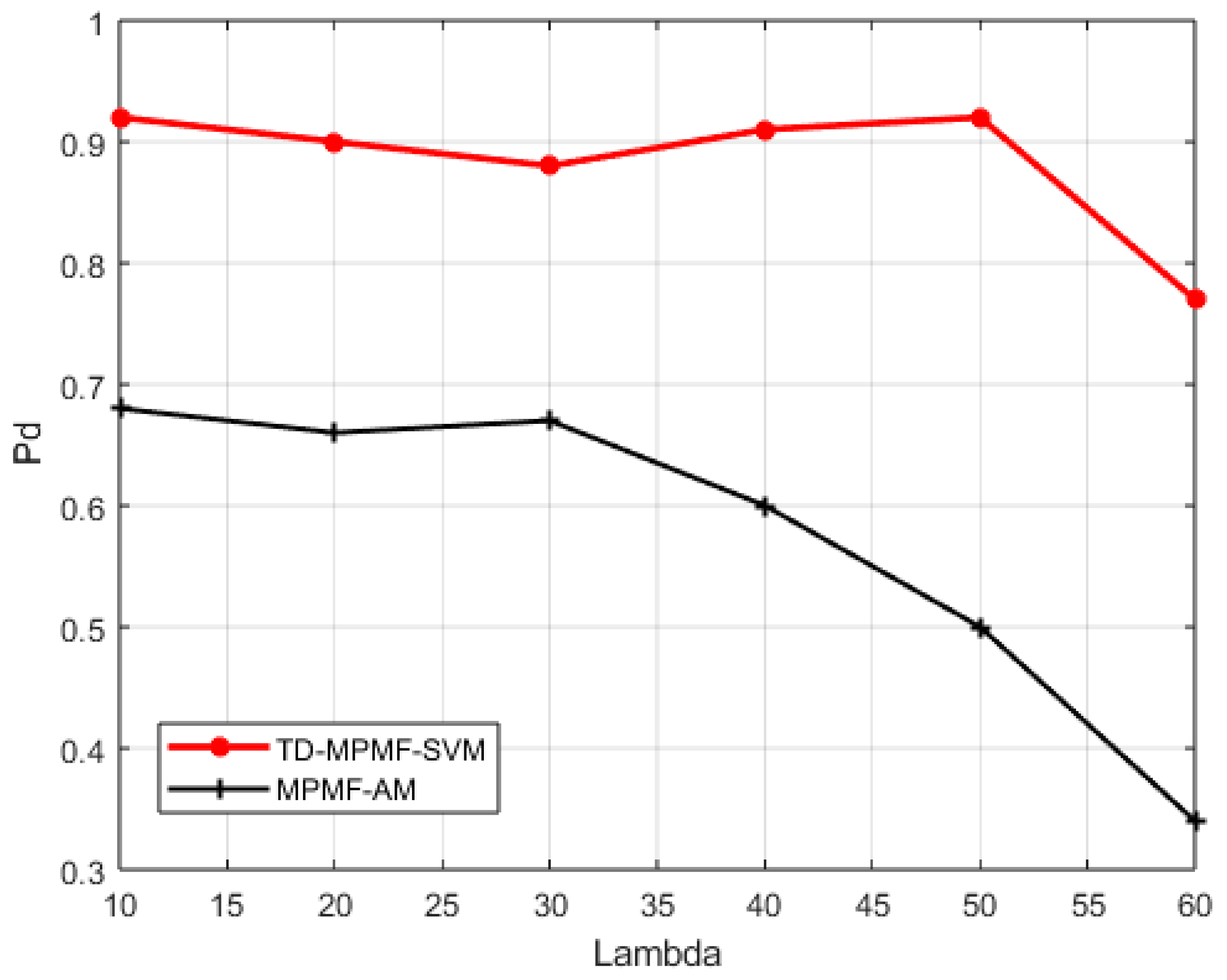
Figure 12 shows the detection probabilities of the two algorithms under different clutter intensities. In various clutter environments, TD-MPMF-SVM maintains a high detection probability and consistently outperforms the MPMF-AM algorithm. When the Poisson intensity ${\lambda }^{\left(p\right)}$ is less than 60, the detection probability of the TD-MPMF-SVM algorithm remains around 0.9.

4.2. Experimental Results

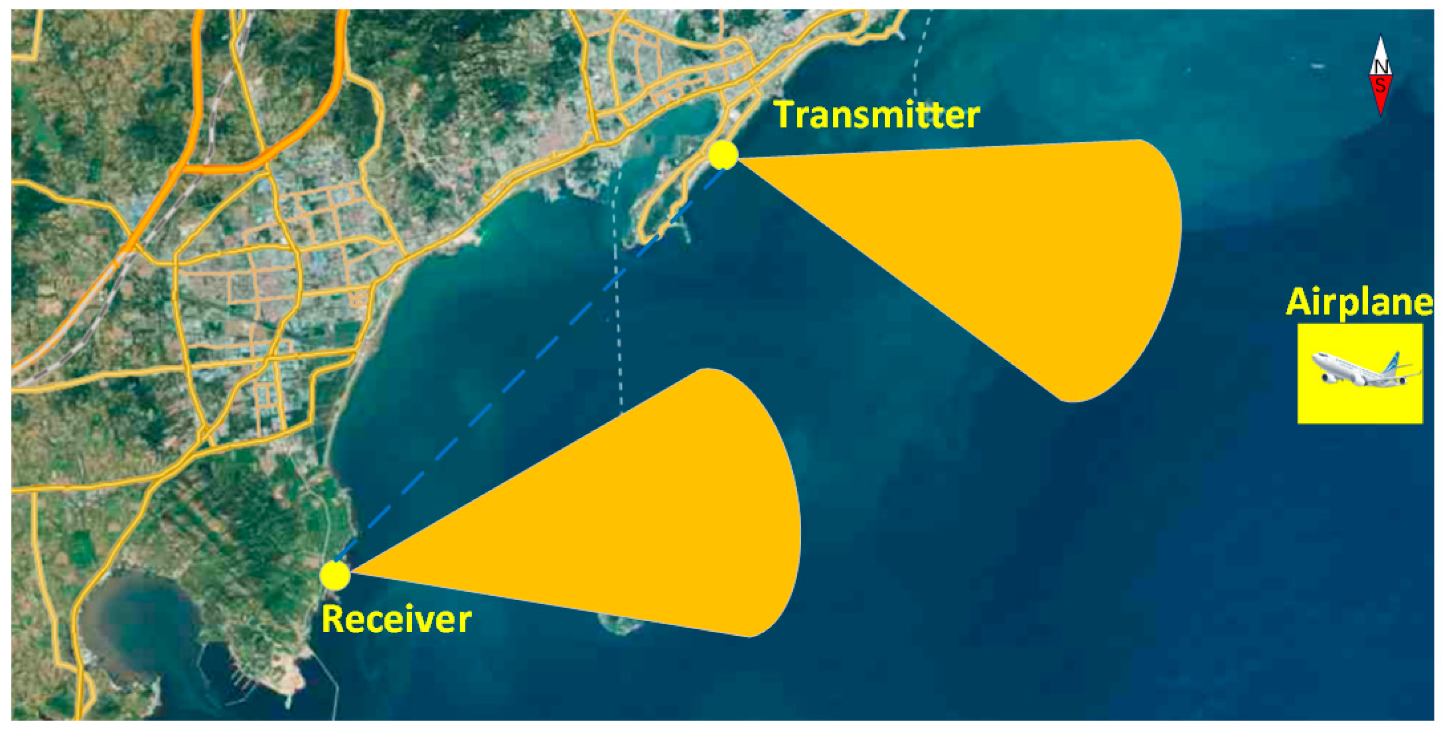
On 22 September 2024, an aircraft detection experiment was conducted in Qingdao, Shandong, China. The experimental scenario is shown in Figure 13, and the radar system parameters are listed in

Table 6. Experimental radar system parameters.

Parameter	Value	Parameter	Value
$f_c$	1.25 GHz	$B$	2 MHz
${PRF}_1$	623.44 Hz	$T_{p1}$	$160.4 \mu \mathrm{s}$
${PRF}_2$	621.89 Hz	$T_{p2}$	$160.8 \mu \mathrm{s}$
${PRF}_3$	515.46 Hz	$T_{p3}$	$194 \mu \mathrm{s}$
${PRF}_4$	512.3 Hz	$T_{p4}$	$195.2 \mu \mathrm{s}$
$f_s$	2.5 MHz	Duty Ratio	0.1

. Both the transmitter and receiver were ground-based platforms and located on the same side of the target. The ground-based receiving platform was oriented toward the target while simultaneously receiving the direct wave signal from the ground-based transmitting platform. The receiving array antenna employed digital beam forming (DBF) technology [32] to achieve multi-channel signal reception.

The number of PRFs of the radar system is $L=4$. Each PRF has a duty ratio of 0.1, and the corresponding azimuth integration time is 0.75 s. Each PRF constitutes a sub-frame. Four PRFs together form a large frame, with an interval of 10 s between consecutive large frames.

1.

Scenario 1

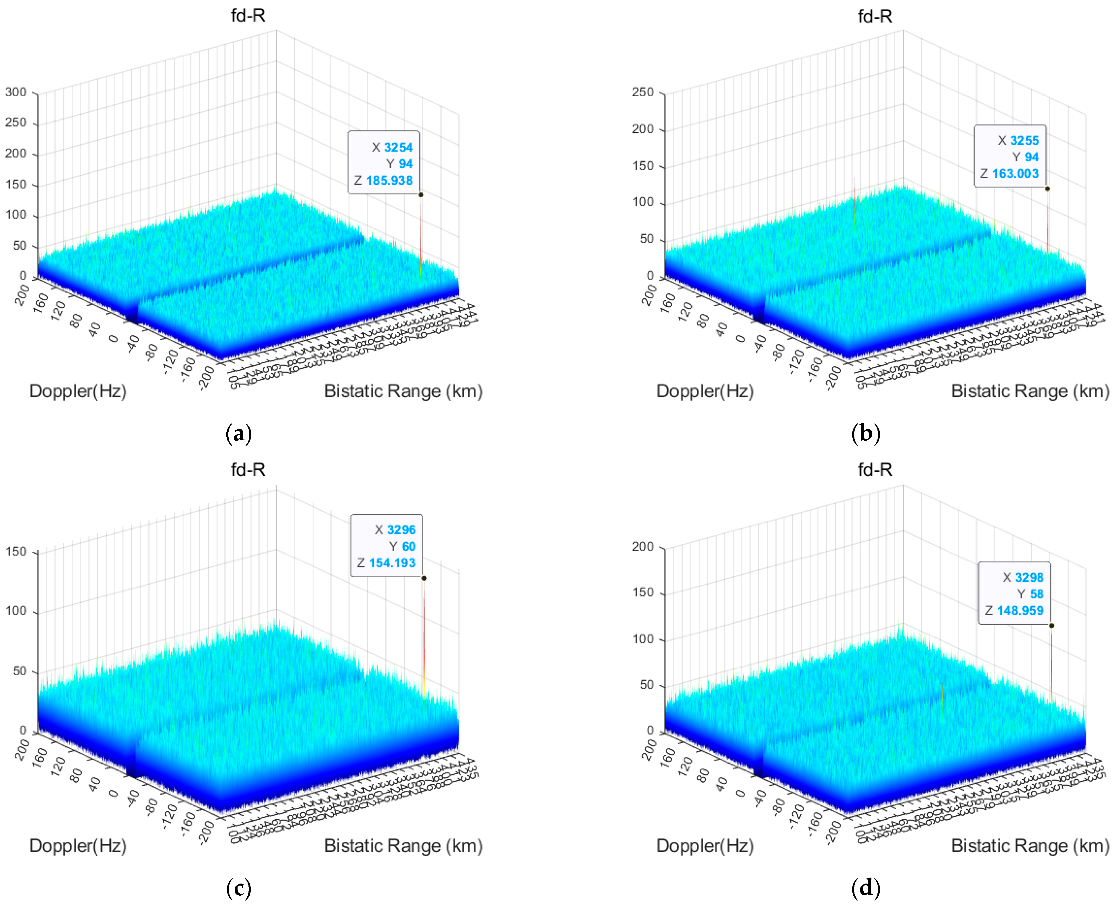
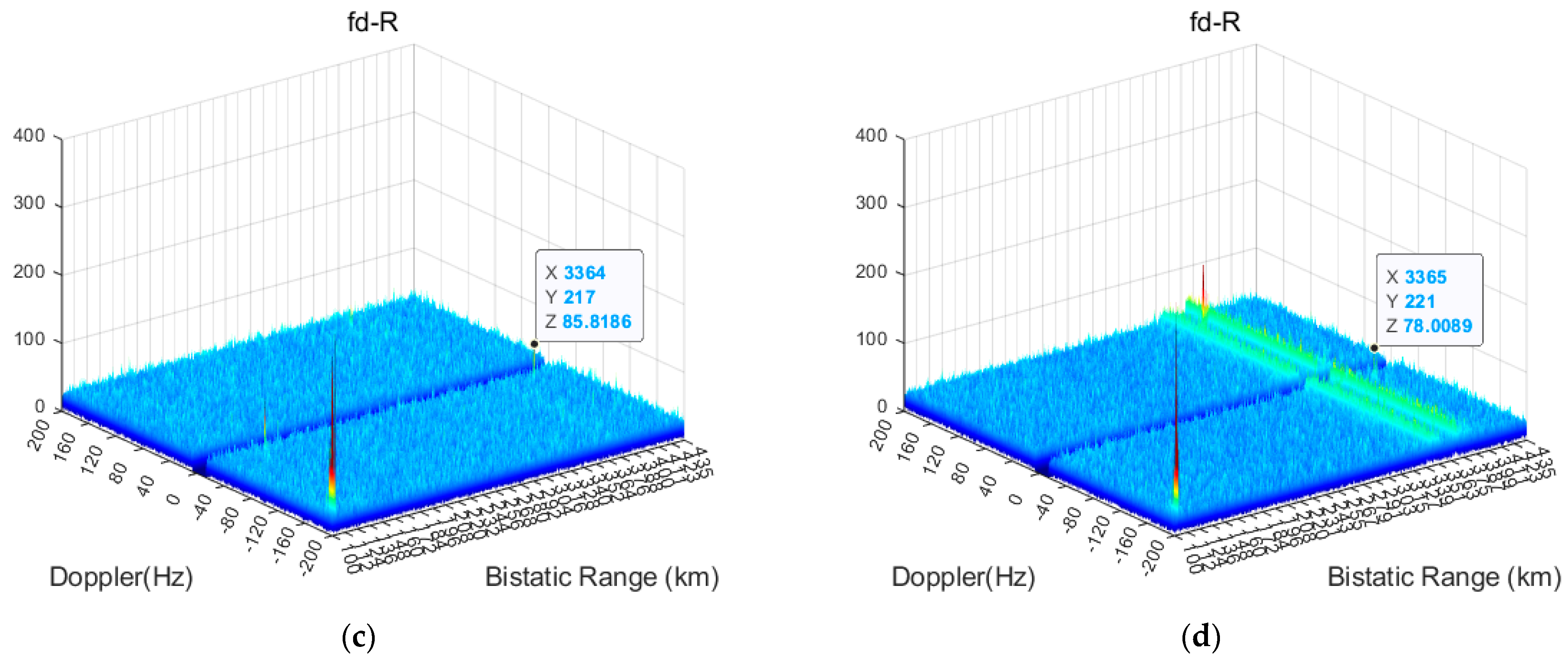
The aircraft maintains approximately CV radial motion while performing cross-beam movement, causing continuous changes in its angle. In frames 13, 14, 15, and 16, the target coherent integration results are shown in Figure 14 and the SNR from CFAR detection is listed in

Table 7. Scenario 1: SNR of CFAR detection output target.

Frame Number	SNR (dB)
13	19.79
14	18.4
15	18.68
16	18.38

.

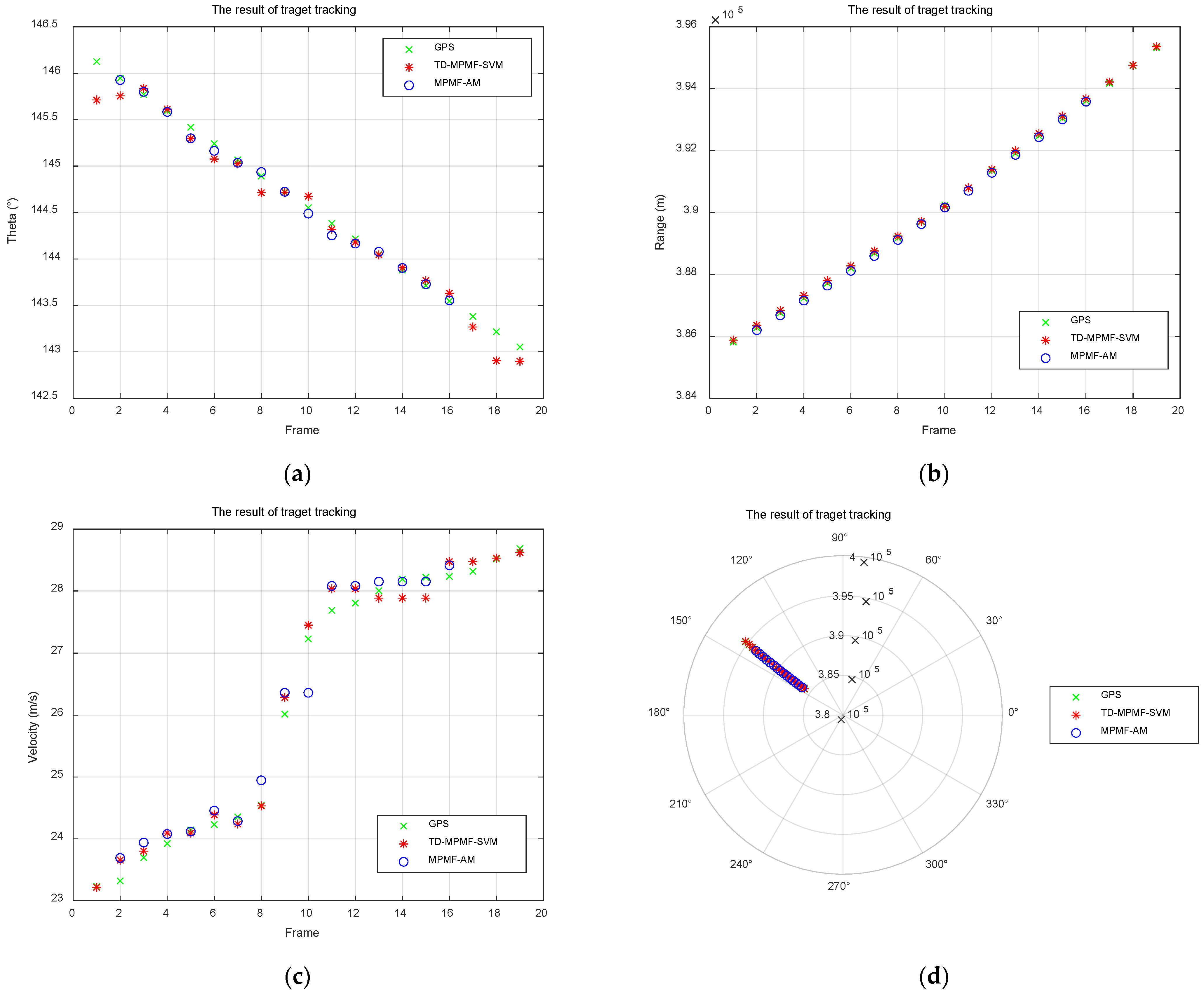
The CFAR detection results are processed using sum-difference beamforming angle estimation to obtain the azimuth angle. The target angle results are shown in Figure 15a. Then, ambiguity resolution is performed to obtain the true distance and true velocity of the target. The true distance results are shown in Figure 15b, while the true velocity results are in Figure 15c. Finally, the Kalman filtering algorithm is applied for target tracking, and the results are shown in Figure 15d.

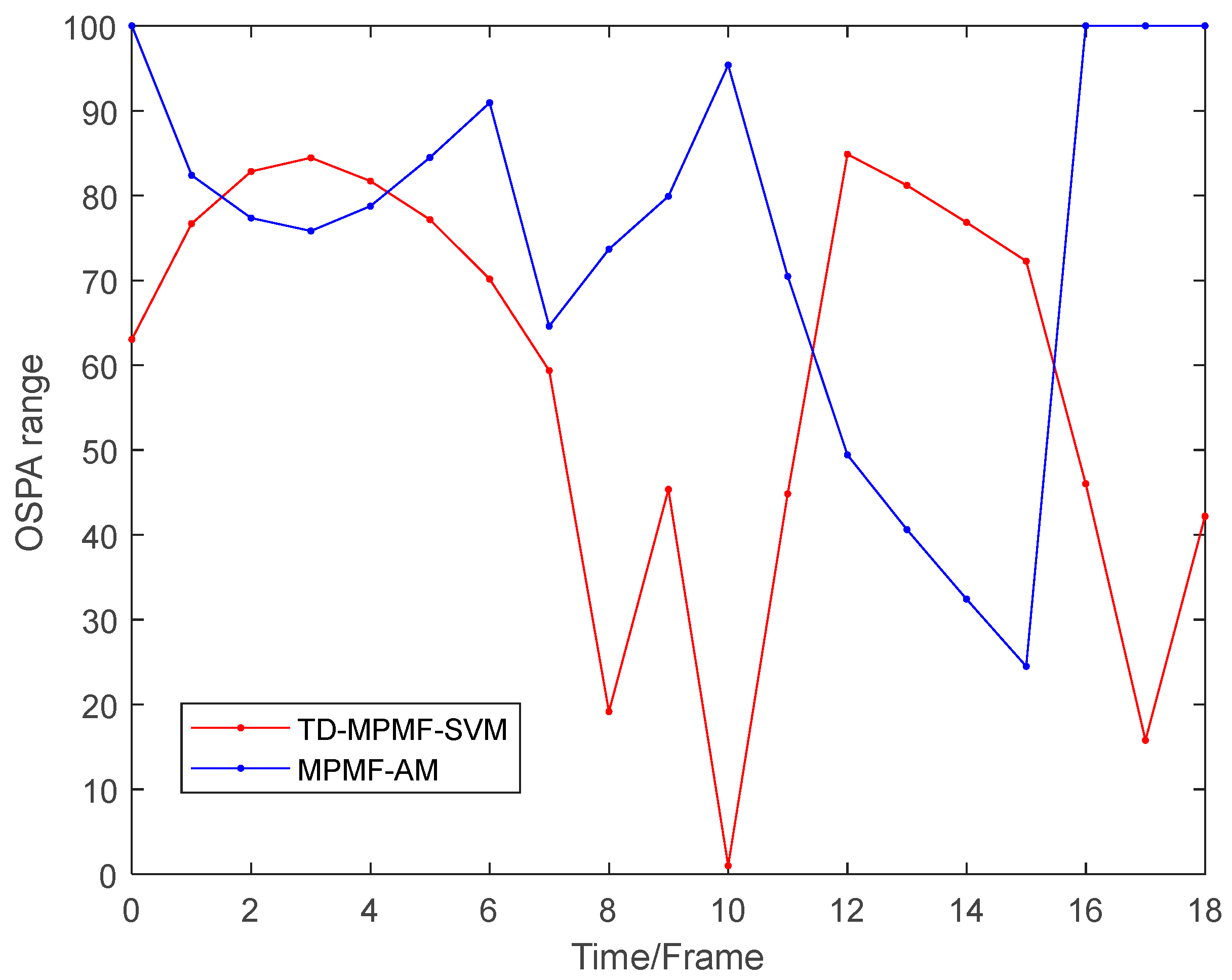
To quantitatively compare the ambiguity resolution and tracking performance of TD-MPMF-SVM and MPMF-AM in MTD, we use OSPA as the evaluation metric, where $c_{cut}$ is 100 m. The results are shown in Figure 16. The mean OSPA for TD-MPMF-SVM is 59.2 m, whereas that for MPMF-AM is 74.77 m. Based on these OSPA results, TD-MPMF-SVM demonstrates superior performance in moving target detection and tracking.

The root mean square error (RMSE) of the range and velocity ambiguity resolution results compared to the true values is shown in

Table 8. Scenario 1: RMSE of ambiguity resolution results.

	Range (m)	Velocity (m/s)
RMSE	64.24	0.2

.

2.

Scenario 2

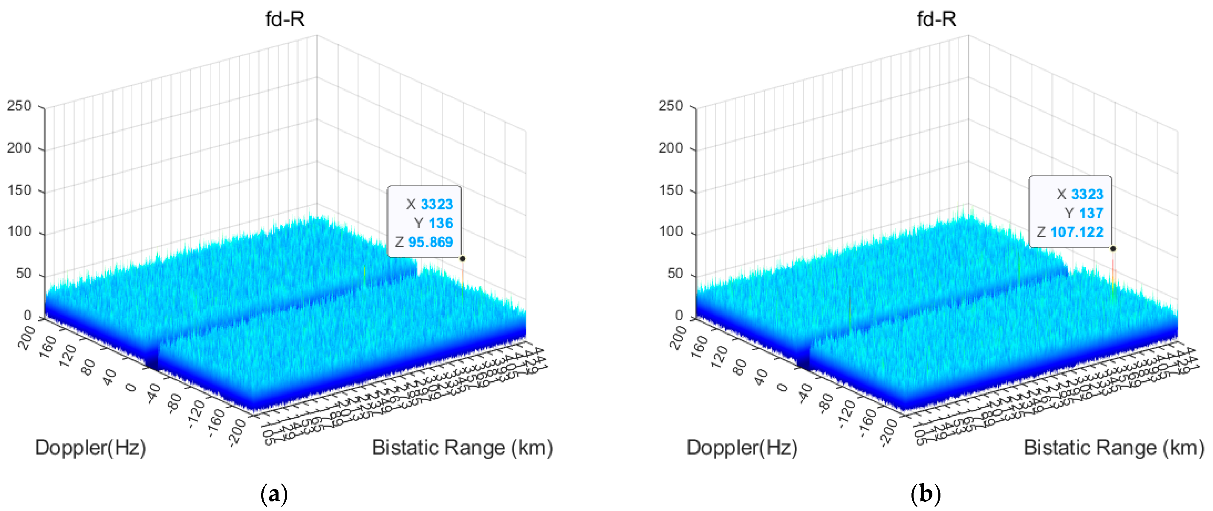
The aircraft moves in a CV radial motion, with the direction of movement pointing towards the receiving platform. In frames 13, 14, 15, and 16, the target coherent integration results are shown in Figure 17, and the CFAR detection SNR is presented in

Table 9. Scenario 2: SNR of CFAR detection output target.

Frame Number	SNR (dB)
13	14.74
14	15.51
15	14.57
16	13.35

.

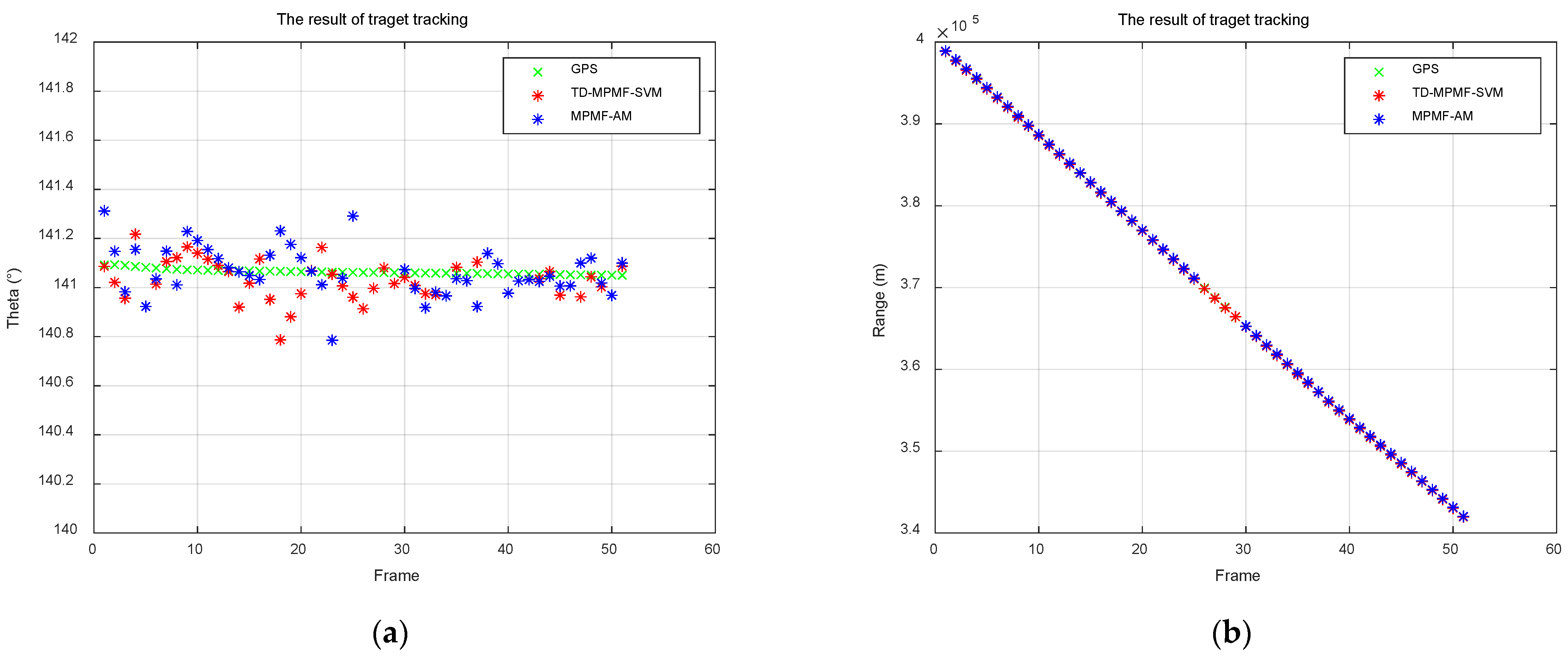
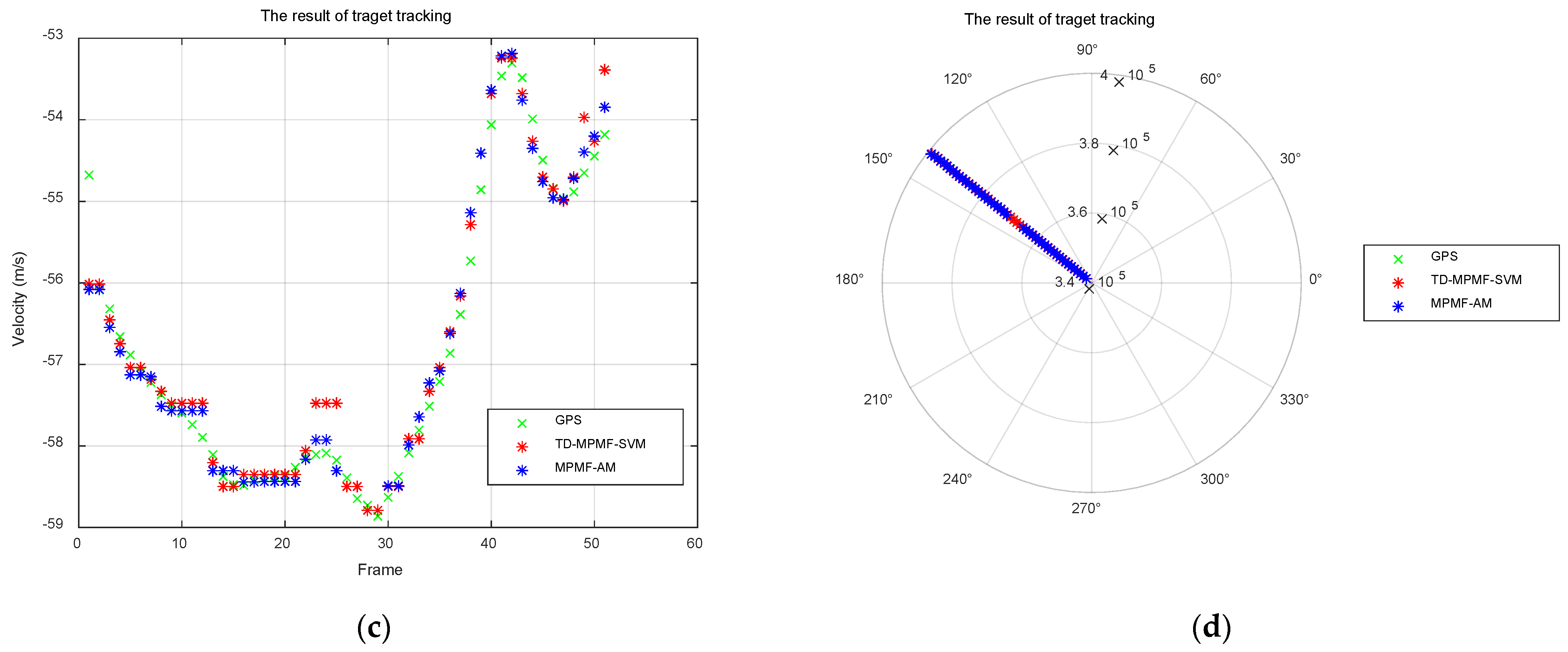
The CFAR detection results are processed using sum-difference beamforming angle estimation to obtain the azimuth angle. The target angle results are shown in Figure 18a. Then, ambiguity resolution is performed to obtain the true distance and true velocity of the target. The true distance results are shown in Figure 18b, and the true velocity results are in Figure 18c. Finally, the Kalman filtering results are shown in Figure 18d.

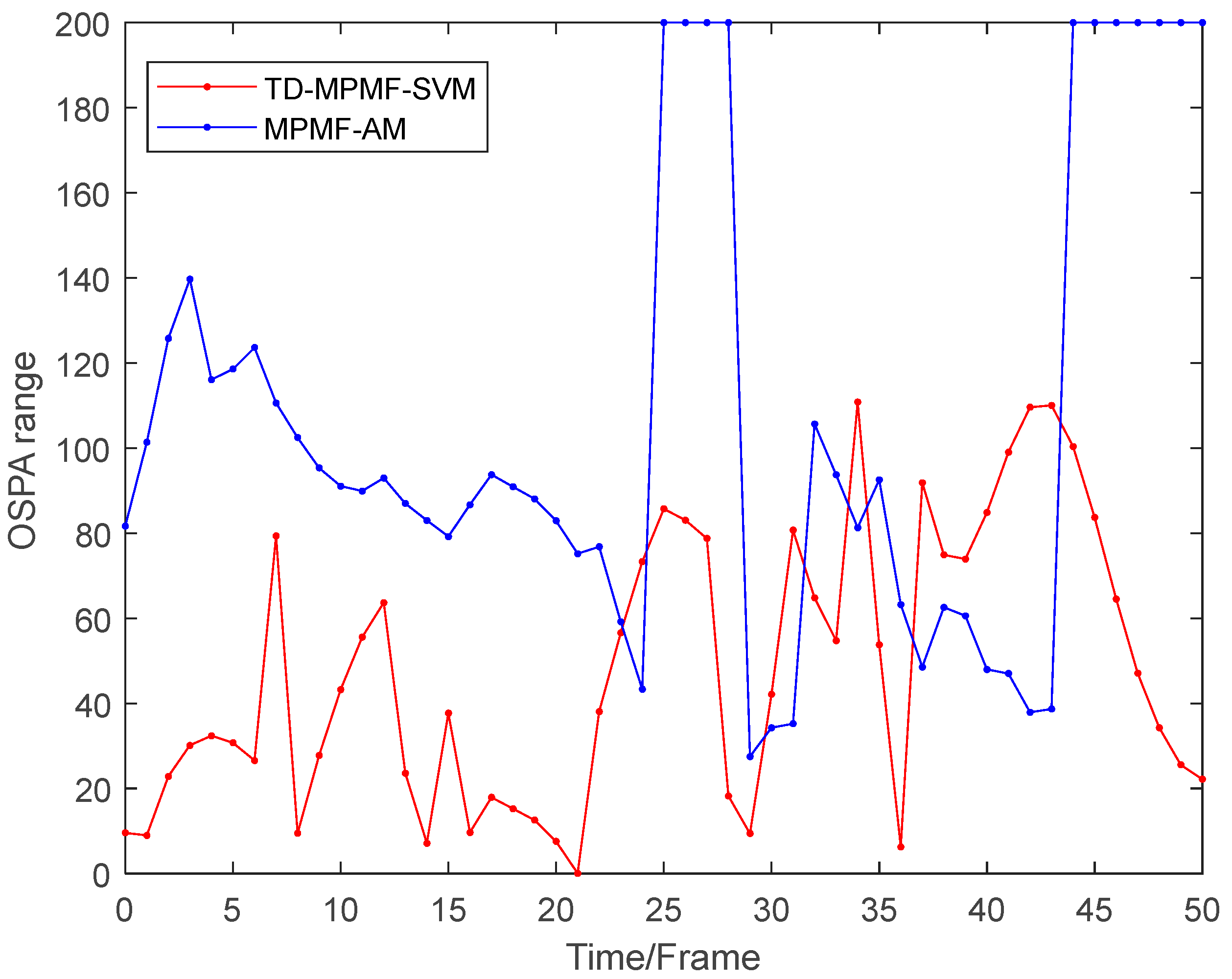
To quantitatively compare the ambiguity resolution and tracking performance of TD-MPMF-SVM and MPMF-AM in MTD, we use OSPA as the evaluation metric, where $c_{cut}$ is 200 m. The results are shown in Figure 19. The mean OSPA for TD-MPMF-SVM is 48.05 m, whereas that for MPMF-AM is 106.12 m. Based on these OSPA results, TD-MPMF-SVM demonstrates superior performance in moving target detection and tracking.

The results for the range and velocity ambiguity resolution results compared to the true values are shown in

Table 10. Scenario 2: RMSE of ambiguity resolution results.

	Range (m)	Velocity (m/s)
RMSE	34.91	0.34

.

5. Conclusions

In this work, the TD-MPMF-based framework for multi-PRF has been proposed, together with the developed TD-MPMF-SVM algorithm. TD-MPMF achieves coherent integration, detection, and tracking of targets in a TD-MPMF system. Intra-frame processing performs block-wise coherent integration, improving processing efficiency while ensuring integration gain. Inter-frame processing utilizes the TD-MPMF-SVM algorithm to decompose the joint simultaneous detection of multiple PRFs into a target detection maximization problem under an MPMF system. Firstly, the TD-MPMF-SVM algorithm expands all possible state values based on the current target state. Secondly, it establishes a target motion model to describe the variation relationship between different frames and PRFs, setting a coarse threshold to filter all target state sequences and obtain potential target sequences. Finally, the target state sequences in the polar coordinate system are transformed into the feature domain and SVM is used to extract the true target state sequence. As demonstrated by computer simulations, the proposed TD-MPMF-SVM algorithm achieves higher accuracy in ambiguity resolution compared to the MPMF-AM algorithm. Moreover, real-world experimental results have also verified the effectiveness of the proposed algorithm.

References

1. Barbary, M.; Zong, P. Novel Anti-Stealth on Sub-Nyquist Scattering Wave Deception Jammer With Stratospheric Balloon-Borne Bistatic Radar Using KA-STAP-FTRAB Algorithm. IEEE Sens. J. 2015, 15, 6437–6453. [Google Scholar] [CrossRef]
2. Ferrari, A.; Berenguer, C.; Alengrin, G. Doppler ambiguity resolution using multiple PRF. IEEE Trans. Aerosp. Electron. Syst. 1997, 33, 738–751. [Google Scholar] [CrossRef]
3. Li, W.; Yi, W.; Wen, M.; Orlando, D. Multi-PRF and multi-frame track-before-detect algorithm in multiple PRF radar system. Signal Process. 2020, 174, 107648. [Google Scholar] [CrossRef]
4. Li, W.; Yi, W.; Kong, L.; Teh, K.C. An Efficient Track-Before-Detect for Multi-PRF Radars With Range and Doppler Ambiguities. IEEE Trans. Aerosp. Electron. Syst. 2022, 58, 4083–4100. [Google Scholar] [CrossRef]
5. Xiong, W.; Lu, Y.; Song, J.; Chen, X. A Two-Stage Track-before-Detect Method for Non-Cooperative Bistatic Radar Based on Deep Learning. Remote Sens. 2023, 15, 3757. [Google Scholar] [CrossRef]
6. Grossi, E.; Lops, M.; Venturino, L. Track-before-detect for multiframe detection with censored observations. IEEE Trans. Aerosp. Electron. Syst. 2014, 50, 2032–2046. [Google Scholar] [CrossRef]
7. Xia, X.G.; Wang, G. Phase Unwrapping and A Robust Chinese Remainder Theorem. IEEE Signal Process. Lett. 2007, 14, 247–250. [Google Scholar] [CrossRef]
8. Trunk, G.; Brockett, S. Range and velocity ambiguity resolution. In Proceedings of the Record of the 1993 IEEE National Radar Conference, Lynnfield, MA, USA, 20–22 April 1993; pp. 146–149. [Google Scholar]
9. Wen, L.; Teng, L.; Yueqiu, H. Resolution of range and velocity ambiguity for a medium pulse Doppler radar. In Proceedings of the Record of the IEEE 2000 International Radar Conference [Cat. No. 00CH37037], Alexandria, VA, USA, 12 May 2000; pp. 560–564. [Google Scholar]
10. Xiao, L.; Xia, X.G.; Wang, Y.P. Exact and Robust Reconstructions of Integer Vectors Based on Multidimensional Chinese Remainder Theorem (MD-CRT). IEEE Trans. Signal Process. 2020, 68, 5349–5364. [Google Scholar] [CrossRef]
11. Xiao, H.; Xiao, G. On Solving Ambiguity Resolution With Robust Chinese Remainder Theorem for Multiple Numbers. IEEE Trans. Veh. Technol. 2019, 68, 5179–5184. [Google Scholar] [CrossRef]
12. Zhu, J.; Li, Y.; Duan, C.; Wang, W.; Wen, C.; Huang, Y. A Range and Velocity Ambiguity Resolution Method Based on Ambiguity Matrix Completion and Elimination with Low SNR. In Proceedings of the 2019 IEEE International Conference on Signal, Information and Data Processing (ICSIDP), Chongqing, China, 11–13 December 2019; pp. 1–6. [Google Scholar]
13. Mao, Y.; Song, C.; Wang, B. Algorithm for the Weak Target Joint Detection and Ambiguity Resolution Based on Ambiguity Matrix. Remote Sens. 2024, 16, 1597. [Google Scholar] [CrossRef]
14. Zhao, P.; Wang, P.; Tang, T.; Ren, Z.; Men, Z. An Improved Range Ambiguity Resolution Algorithm for GNSS-Based Bistatic Radar Target Detection. In Proceedings of the IGARSS 2024—2024 IEEE International Geoscience and Remote Sensing Symposium, Athens, Greece, 7–12 July 2024; pp. 7685–7688. [Google Scholar]
15. Hovanessian, S.A. Medium PRF Performance Analysis. IEEE Trans. Aerosp. Electron. Syst. 1982, AES-18, 286–296. [Google Scholar] [CrossRef]
16. Alabaster, C.M.; Hughes, E.J.; Matthew, J.H. Medium PRF radar PRF selection using evolutionary algorithms. IEEE Trans. Aerosp. Electron. Syst. 2003, 39, 990–1001. [Google Scholar] [CrossRef]
17. Luo, J.; Huang, Y.; Mao, D.; Zhang, Y.; Zhang, Y.; Yang, J. Azimuth–Elevation Forward-Looking Super-Resolution Imaging Based on Sparse Doppler Phase Convolution Model for High-Speed Platform. IEEE Trans. Geosci. Remote Sens. 2024, 62, 5110118. [Google Scholar] [CrossRef]
18. Tang, T.; Wang, P.; Chen, J.; Zhao, P.; Ren, Z.; Zeng, H. A Time-Frequency Synchronization Method Using Dual-Channel Processing For GNSS-Based Passive Radar Moving Target Detection. In Proceedings of the IGARSS 2024—2024 IEEE International Geoscience and Remote Sensing Symposium, Athens, Greece, 7–12 July 2024; pp. 6368–6371. [Google Scholar]
19. Sun, W.; Xu, H.; Wu, S. A Novel Compensation Method to Calibrate Dispersion Effect for Spaceborne Synthetic Aperture Radar. In Proceedings of the 2024 IEEE International Conference on Signal, Information and Data Processing (ICSIDP), Zhuhai, China, 22–24 November 2024; pp. 1–5. [Google Scholar]
20. Fang, Y.; Atkinson, G.; Sayin, A.; Chen, J.; Wang, P.; Antoniou, M.; Cherniakov, M. Improved Passive SAR Imaging With DVB-T Transmissions. IEEE Trans. Geosci. Remote Sens. 2020, 58, 5066–5076. [Google Scholar] [CrossRef]
21. Yu, J.; Pan, B.; Yu, Z.; Zhu, H.; Li, H.; Li, C.; Sun, H. Sea Clutter Suppression Based on Chaotic Prediction Model by Combining the Generator and Long Short-Term Memory Networks. Remote Sens. 2024, 16, 1260. [Google Scholar] [CrossRef]
22. Wang, H.; Lujing, C. On adaptive spatial-temporal processing for airborne surveillance radar systems. IEEE Trans. Aerosp. Electron. Syst. 1994, 30, 660–670. [Google Scholar] [CrossRef]
23. Kronauge, M.; Rohling, H. Fast Two-Dimensional CFAR Procedure. IEEE Trans. Aerosp. Electron. Syst. 2013, 49, 1817–1823. [Google Scholar] [CrossRef]
24. He, Y.D.; Zhou, J.; Zhou, B.H. Adaptive Sum and Difference Beamforming for Monopulse System with Array Antennas. In Proceedings of the 2010 6th International Conference on Wireless Communications Networking and Mobile Computing (WiCOM), Chengdu, China, 23–25 September 2010; pp. 1–5. [Google Scholar]
25. Xu, Z.; Xiong, Z.; Wu, J.; Xiao, S. Symmetrical difference pattern monopulse for low-angle tracking with array radar. IEEE Trans. Aerosp. Electron. Syst. 2016, 52, 2676–2684. [Google Scholar] [CrossRef]
26. Chen, S.; Zhao, Y.; Hu, Y.; Pang, X. Beamspace Maximum Likelihood Algorithm Based on Sum and Difference Beams for Elevation Estimation. J. Syst. Eng. Electron. 2024, 35, 589–598. [Google Scholar] [CrossRef]
27. Zhang, H.; Liu, W.; Zhang, Q.; Zhang, L.; Liu, B.; Xu, H.X. Joint Power, Bandwidth, and Subchannel Allocation in a UAV-Assisted DFRC Network. IEEE Internet Things J. 2025, 12, 11633–11651. [Google Scholar] [CrossRef]
28. Zhang, H.; Liu, W.; Zhang, Q.; Liu, B. Joint Customer Assignment, Power Allocation, and Subchannel Allocation in a UAV-Based Joint Radar and Communication Network. IEEE Internet Things J. 2024, 11, 29643–29660. [Google Scholar] [CrossRef]
29. Zhang, H.; Liu, W.; Zhang, Q.; Fei, T. A robust joint frequency spectrum and power allocation strategy in a coexisting radar and communication system. Chin. J. Aeronaut. 2024, 37, 393–409. [Google Scholar] [CrossRef]
30. Schuhmacher, D.; Vo, B.T.; Vo, B.N. A Consistent Metric for Performance Evaluation of Multi-Object Filters. IEEE Trans. Signal Process. 2008, 56, 3447–3457. [Google Scholar] [CrossRef]
31. Vo, B.T.; Vo, B.N.; Cantoni, A. The Cardinality Balanced Multi-Target Multi-Bernoulli Filter and Its Implementations. IEEE Trans. Signal Process. 2009, 57, 409–423. [Google Scholar] [CrossRef]
32. Tian, Z.; Yu, Z.; Guo, Y.; Yu, J.; Li, D. Azimuth Multichannel SAR Imaging Algorithm Based on Spectral Extrapolation and Image Fusion. IEEE Trans. Geosci. Remote Sens. 2024, 62, 5219815. [Google Scholar] [CrossRef]
Figure 1. The scenario using the TD-MPMF bistatic radar system.
Remotesensing 17 03583 g001
Figure 2. The geometric relationship of the TD-MPMF bistatic radar system.
Remotesensing 17 03583 g002
Figure 3. Radar data structure.
Remotesensing 17 03583 g003
Figure 4. Processing flow-chart of the TD-MPMF method.
Remotesensing 17 03583 g004
Figure 5. Block diagram of the TD-MPMF-SVM algorithm.
Remotesensing 17 03583 g005
Figure 6. Multi-PRF measurement data.
Remotesensing 17 03583 g006
Figure 7. SVM fine-stage procedure.
Remotesensing 17 03583 g007
Figure 8. Target coherent integration results: (a) k = 80; (b) k = 81; (c) k = 82; (d) k = 83.
Remotesensing 17 03583 g008
Figure 9. When λ ( p ) = 20 , the ambiguity resolution results of the TD-MPMF-SVM algorithm and the MPMF-AM algorithm are presented: (a) range results; (b) velocity results.
Remotesensing 17 03583 g009
Figure 10. When λ ( p ) = 20 , OSPA distance of TD-MPMF-SVM and MPMF-AM algorithms is presented.
Remotesensing 17 03583 g010
Figure 11. OSPA distance of TD-MPMF-SVM and MPMF-AM algorithms under different Poisson intensities λ ( p ) .
Remotesensing 17 03583 g011
Figure 12. Detection probabilities of TD-MPMF-SVM and MPMF-AM algorithms under different Poisson intensities λ ( p ) .
Remotesensing 17 03583 g012
Figure 13. Experimental scene description.
Remotesensing 17 03583 g013
Figure 14. Scenario 1: Target coherent integration results: (a) k = 13, (b) k = 14, (c) k = 15, (d) k = 16.
Remotesensing 17 03583 g014
Figure 15. Scenario 1: (a) angle measurement results, (b) range ambiguity resolution results, (c) velocity ambiguity resolution results, (d) target track results.
Remotesensing 17 03583 g015
Figure 16. Scenario 1: OSPA distance of TD-MPMF-SVM and MPMF-AM algorithms.
Remotesensing 17 03583 g016
Figure 17. Scenario 2: Target coherent integration results: (a) k = 13, (b) k = 14, (c) k = 15, (d) k = 16.
Remotesensing 17 03583 g017aRemotesensing 17 03583 g017b
Figure 18. Scenario 2: (a) angle measurement results, (b) range ambiguity resolution results, (c) velocity ambiguity resolution results, (d) target track results.
Remotesensing 17 03583 g018aRemotesensing 17 03583 g018b
Figure 19. Scenario 2: OSPA distance of TD-MPMF-SVM and MPMF-AM algorithms.
Remotesensing 17 03583 g019