Filter-Wise Mask Pruning and FPGA Acceleration for Object Classification and Detection

Highlights

What are the main findings?

• A novel filter-wise mask pruning approach is proposed, which achieves the benefits of both unstructured and structured pruning. The newly introduced structural constraint on the filter dimension leads to more regularity, generating more hardware-friendly and performant models.
• An FMP-based acceleration architecture is proposed for real-time processing. The strategy for calculation parallelism and memory access is dedicatedly optimized to enhance workload balance and throughput.

What are the implications of the main findings?

• The proposed pruning method is proven on both classification networks and detection networks. The pruning rate can achieve 75.1% for VGG-16 and 84.6% for ResNet-50 without accuracy compromise. The pruned YOLOv5s achieves a pruning rate of 53.43% with a slight accuracy degradation of 0.6%.
• The proposed acceleration architecture is implemented on FPGA to evaluate its practical execution performances. The throughput reaches up to 809.46MOPS. The pruned network achieves the speedup of 2.23× and 4.4×, with a compression rate of 2.25× and 4.5×, respectively, converting the model compression to the execution speedup effectively.

Abstract

Pruning and acceleration has become an essential and promising technique for convolutional neural networks (CNN) in remote sensing image processing, especially for deployment on resource-constrained devices. However, how to maintain model accuracy and achieve satisfactory acceleration simultaneously remains to be a challenging and valuable problem. To break this limitation, we introduce a novel pruning pattern of filter-wise mask by enforcing extra filter-wise structural constraints on pattern-based pruning, which achieves the benefits of both unstructured and structured pruning. The newly introduced filter-wise mask enhances fine-grained sparsity with more hardware-friendly regularity. We further design an acceleration architecture with optimization of calculation parallelism and memory access, aiming to fully translate weight pruning to hardware performance gain. The proposed pruning method is firstly proven on classification networks. The pruning rate can achieve 75.1% for VGG-16 and 84.6% for ResNet-50 without accuracy compromise. Further to this, we enforce our method on the widely used object detection model, the you only look once (YOLO) CNN. On the aerial image dataset, the pruned YOLOv5s achieves a pruning rate of 53.43% with a slight accuracy degradation of 0.6%. Meanwhile, we implement the acceleration architecture on a field-programmable gate array (FPGA) to evaluate its practical execution performance. The throughput reaches up to 809.46MOPS. The pruned network achieves a speedup of 2.23× and 4.4×, with a compression rate of 2.25× and 4.5×, respectively, converting the model compression to execution speedup effectively. The proposed pruning and acceleration approach provides crucial technology to facilitate the application of remote sensing with CNN, especially in scenarios such as on-board real-time processing, emergency response, and low-cost monitoring.

1. Introduction

Real-time processing in remote sensing has been evolving rapidly, driven by collaborative breakthroughs in remote sensing detectors, computing technology, algorithm and hardware upgrades [1,2,3,4]. With remote sensing processing transitioning from “post hoc analysis” to “in situ intervention”, the edge intelligence plays more and more essential roles [2]. However, the harsh restrictions on computing resources and power, whether on on-orbit satellites or unmanned aerial vehicles (UAV), impose stringent limitations on the size and complexity of CNN models [5,6,7].

To overcome this hurdle, plenty of prior works are intensively studied to reduce model size and accelerate computation simultaneously, on hardware platforms including graphics processing units (GPUs) [8,9,10], field-programmable gate arrays (FPGAs) [11,12,13] and application-specific integrated circuits (ASICs) [14,15,16]. Benefiting from the significant redundancy of the parameterization of CNNs, the sparsity-centric pruning techniques have achieved outstanding results by exploiting the sparsity of weights [17,18] or activations [19,20,21].

Among them, weight pruning has drawn more study attention. Early efforts mainly relied on iterative and heuristic methods [22,23,24]; for instance, Han et al. [25] reported that top-K pruning achieves a reduction in the number of weights by a factor of 13×, with an accuracy degradation of less than 1%. Despite the high sparsity, the sparse networks do not guarantee high improvement in hardware-level performance, such as CNN inference acceleration. Specifically, the general but unstructured weight pruning, with a random number of non-zero elements, barely takes advantage of vector-processing architectures and memory buses, often leading to a poor workload and preventing high parallelism [26]. Moreover, the indices for the generic sparse matrix representation impedes the weight storage and throughput. For example, though the compressed sparse row (CSR) format [27] is helpful to save index storage, the decoding of the index requires a search over the whole activation vector, bringing little acceleration and even speed degradation. Both the above-mentioned overheads pose great challenges in hardware implementation.

Contrary to irregular pruning, structural pruning can generate more hardware-friendly models by reducing the network complexity at a coarse-grained level, including vector-wise pruning, kernel-wise pruning, channel-wise pruning, and filter-wise pruning [28]. Figure 1 illustrates the pruning methods on weight matrix with a shape of 4 × 3 × 3 × 3. Consequently, the pruned network keeps the original structure, which is well-fitted to regular hardware, to obtain performance gain. Nonetheless, such methods suffer more accuracy degradation as the increment of pruning granularity. Taking [29] as an example, Alex Renda et al. achieved 9.31× compression with 1% accuracy loss when using unstructured pruning, while a similar accuracy performance could only be maintained at 1.70× compression in filter pruning.

To address the performance issue, pattern pruning methods [30,31,32] have been proposed for a better compromise between hardware efficiency and accuracy, which explore an intermediate sparse dimension. With fine-grained pruning patterns inside coarse-grained structures, pattern pruning methods guarantee the uniform count of residual weights in convolutional kernels, to the benefit of thread synchronization and workload balance. Tan et al. [32] achieved a compression rate of up to 8.4×, with only 0.2% accuracy loss on the specific hardware accelerator. It can be observed that, although the indices’ storage is relatively reduced, the total throughput of feature data and weight is not improved, and the calculation pipeline is not compressed sufficiently with the high compression rate. Additionally, the optimizations, e.g., kernel reordering, perform on-the-fly and take time. Thus, an exploration space still remains between sparsity regularity and practical speedup in hardware deployment.

Besides the study on general-purpose deep learning compression, plenty of works focus on high-accuracy detection models. Lightweight and compact structures are designed to improve large-scale networks with a lightweight cross stage partial (L-CSP) module [33] and an L-Ghost EMO module [34]. Weight pruning is also an extensive compression approach for detection models. Ma et al. [35] perform sparsity training by applying ${\mathcal{l}}_1$-norm regularization to the channel-scaling factors to find less important channels and layers for YOLOv4. Utilizing the channel pruning strategy, a lightweight YOLOv7 model achieves a high level of accuracy for human detection on portable devices [36]. As far as we know, the structured pruning techniques, such as channel-wise and filter-wise pruning, draw the most attention to accelerate the detection task, while the application and evaluation of finer-grained pruning is worth more exploration.

In this paper, we propose the filter-wise mask pruning (FMP) method, which enforces extra filter-wise structural constraints on pattern-based pruning, and an acceleration architecture is further put forward. Compared with the prior pattern pruning methods [31,32,37], the reinforced structural regularity brings three merits: (1) Benefitting from the feature that all the kernels in the identical input channel among the filters share the same input feature map, and the filter-wise structural constraint keeps the correspondence relation between the data and weights. Consequently, only the unpruned weights and data are fetched and fed into MACs, streaming without interruption by invalid data, while the output channels compute concurrently. That means the transferring and computing time originally used for pruned weights can be eliminated correspondingly, speeding up the model inference process. (2) With the data shared among the filters, only one input feature map buffer is needed in the on-chip memory allocation. The weight buffer overhead is remarkably reduced, since only the unpruned weights are cached. (3) In acceleration architecture, the control logic is simplified, thus reducing logic resource consumption. The sparse matrix encoding/decoding strategy is simplified due to the limited and shared patterns among the filters. The controllers for input and output buffers can be shared in multiple parallel channels, due to identical scheduling. The implementation of filter-wise mask pruning consists of two stages: (1) sparse matrix generating, through filter-wise mask setting up, group lasso regularization and fine-tune, and (2) model execution of acceleration architecture with optimization for the data path and parallel computing.

Experiment results demonstrate the effectiveness of the proposed pruning method and acceleration architecture. The accuracy performance of our pruning method is firstly proven on classification networks. We achieve a pruning rate of 75.1% for VGG-16 and 84.6% for ResNet-50, with even a small accuracy promotion by 0.04% and 0.07%, respectively. Further to this, with a grazing livestock dataset established on UAV images, we investigate the pruning performances on the object detection model, YOLOv5. We also implement the FMP-based acceleration architecture on an FPGA platform, achieving the maximum throughput, up to 809.46MOPS. When the network is pruned with a compression rate of 2.25× and 4.5×, it can achieve speedups of 2.23× and 4.4×, respectively, exhibiting a promising execution acceleration.

The key contributions of this paper include:

• Aiming for efficient model compression, a novel filter-wise mask pruning approach is proposed, which achieves the benefits of both unstructured and structured pruning. Besides the fine-grained pattern pruning, the newly introduced structural constraint on filter dimension leads to more regularity, generating more hardware-friendly and performant models.
• We further propose FMP-based acceleration architecture for real-time processing. Aiming for efficient streaming computing, the strategy for calculation parallelism and memory access are dedicatedly optimized to enhance workload balance and throughput, which fully translates weight pruning to hardware performance gain.
• We conduct extensive experiments on various remote sensing tasks, including VGG-16 and ResNet-50 for object classification and YOLOv5 for object detection, providing benchmarks and tricks for sparse network generation. The proposed acceleration architecture is implemented in FPGA, achieving a high-performing speedup.

The remainder of this paper is organized as follows. Section 2 presents the methodology and design of filter-wise mask pruning and details about the FMP-based acceleration architecture. Furthermore, in Section 3, we present the evaluation of the proposed method and the implementation of the acceleration architecture in FPGA. In Section 4, a general discussion including the future promotion of this work is presented. Finally, Section 5 concludes the highlights and achievements of the work.

2. Materials and Methods

2.1. Filter-Wise Mask Pruning

In this subsection, we introduce the pruning pattern of filter-wise mask, in which all filters share an identical sparsity mask. Further to this, the methodology and its implementation details are presented in the subsections below. Our approach is a noteworthy example of hardware/software co-design that achieves an excellent inference speedup and accuracy performance.

An excellent hardware performance depends on both the high-speed computation and lower memory access. Although plenty of prior works have been conducted in structured/unstructured weight pruning, the significant design space remains for a valuable tradeoff between execution efficiency and prediction quality. To achieve the goal, we explore a more effectual spatial constraint on the weight matrix, which seeks a balance between structural flexibility and regularity. Flexibility is a vital guarantee for accuracy retention; meanwhile, better regularity enables more efficient hardware execution. Inspired by the fine-grained pruning patterns [31], we apply identical pattern masks among the filters, but the pattern differs in the kernels in one filter to avoid huge flexibility degradation. We want to stress that the improvement of the sparsity pattern not only converts the compression rate to computation reduction effectively but also lessens the memory bandwidth pressure. Designed for parallel acceleration, our method is appliable to FPGAs and GPUs.

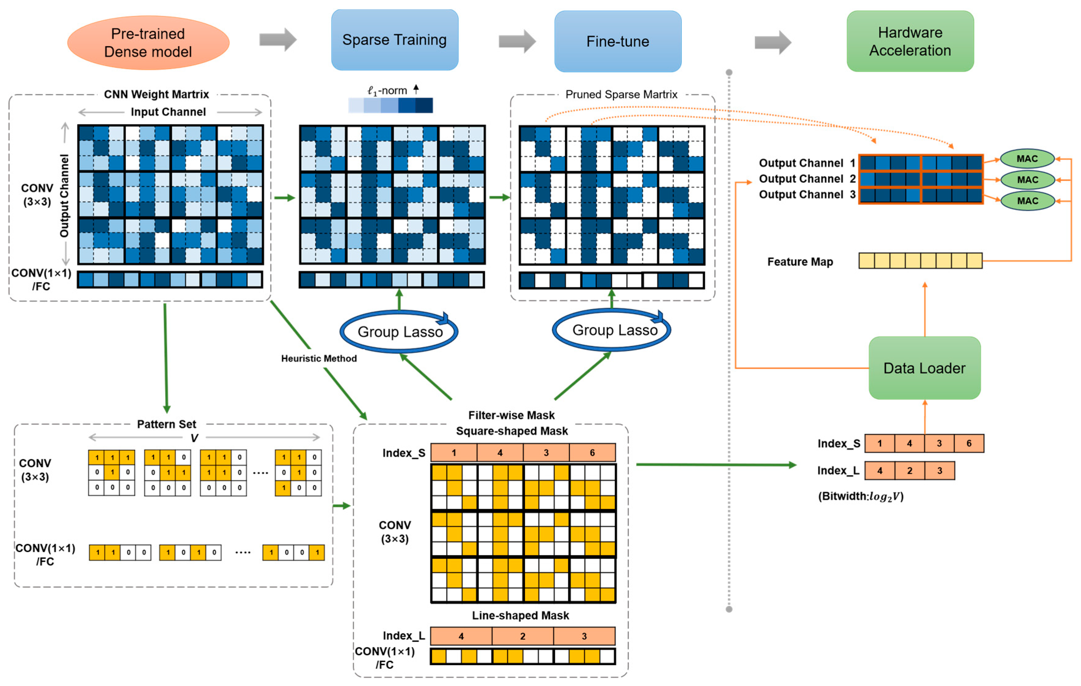
The overall flow of FMP is illustrated in Figure 2, which is composed of four stages. First, a mask set is established, containing the most valuable pattern masks, which are detailed in the next subsection. Different mask subsets correspond to different kernel sizes, as the example in Figure 2 demonstrates, in which the square-shaped masks are for the most commonly used kernels (e.g., size of 3 × 3, 7 × 7) in CONV layers and the line-shaped masks are for 1 × 1 kernels in FC layers. Given the total number of patterns $V$, the width of indices can be limited to ${\log }_{2}V$. With each index corresponding to a specific pattern style, the cumbersome decoding process can be simplified. In the second stage, the pattern masks are applied to the pre-trained dense model, and the sparse training is conducted. Consequently, the weights inside the masks can be learned higher and others are enforced to near-zero, which will be removed in the pruning process. This is helpful to avoid a severe accuracy penalty. Subsequently, pruning the regularized weights with masks, the sparse model is fine-tuned to recover accuracy. In the last stage, the hardware acceleration is conducted based on the pruned weight matrix and its corresponding indices. The data-path and parallel computing are optimized, which is detailed in Section 2.2.

2.1.1. Design of Filter-Wise Mask

Here, we define the problem of deriving the filter-wise mask. Let us first focus on the pruning patterns. Considering the most common 3 × 3 kernels, if we set the number of preserved weights in a kernel to be $U$, the total number of possible patterns could be $\left(\begin{array}{c}9\\ U\end{array}\right)$. Actually, a large proportion of them are redundant; thus, we employ the heuristic algorithm to search for the candidate pattern set. Firstly, we scan the whole pre-trained CNN model to find all the possible patterns that fit for each kernel. Then, we count the numbers for each pattern and further select the top V patterns with the highest appearance frequency. Hence, the pattern set adapter to the model is formed, denoted as $\mathit{P}=\{P_v:0<v\le V\}$. The empirical number of the valuable patterns can be limited to less than 16 without obvious accuracy drops [32].

In recent studies, smaller convolutional kernels (e.g., 1 × 1) have been adopted to develop light-weight networks. Therefore, we import the N:M structured sparsity [37,38] to form a line-shaped pattern, which is more suitable for 1 × 1 convolutional kernels. Regarding the FC layers to be special CONV layers, the pruning methodology is also applicable, and in the following contents they will not be discussed individually, to simplify the explanations.

Next, we explain how we generate the filter-wise mask for the network. With a given L-layer CNN model, we denote the collection of weights in the l-th layer as a 4D tensor $W^l\in {\mathbb{R}}^{N_l\times C_l\times H_l\times D_l}$, where $N_l$, $C_l$, $H_l$ and $D_l$ represent the number of the output channels, the number of kernels, the height of the kernel and the width of the kernel, respectively. The collection of all weights in the network is $\mathit{W}=\{W^l:0<l\le L\}$. We denote $W_{n,c}^l$ as the c-th kernel in the n-th filter in the l-th layer for simplicity.

Network pruning can be defined as imposing a sparsity mask $\mathit{\Omega }$ upon $\mathit{W}$, where $\mathit{\Omega }$ is a binary tensor with the same dimensions as $\mathit{W}$. The sparse network can be formulated as follows:

$$\tilde{\mathit{W}}=\mathit{W}\odot \mathit{\Omega },$$

(1)

$$s.t. {\mathit{ }\mathit{\Omega }=\{\Omega }_{n,c}^l:0<l\le L, 0<c\le C_l, 0<n\le N_l\},$$

$${\Omega }_{n,c}^l\in \mathit{P}.$$

where $\odot$ denotes Hadamard product.

For the filter-wise mask, since all the filters share an identical filter mask, $\mathit{\Omega }$ can be regarded as a sequence of filter mask ${\overline{\Omega }}^l$, every element of which is a distinct kernel mask, $i.e., {\Omega }_{:,c}^l={\overline{\Omega }}_c^l, c=1,\dots ,C_l$. Since the criteria to identify the important weights by weight and gradient has been proven to have a superior performance [39,40,41], we take this into consideration when optimizing the sparsity mask. The mask optimization can be expressed as follows:

$${\displaystyle \frac{\arg \max }{{\overline{\Omega }}_c^l}} {‖W_{:,c}^l\odot g(W^l)\odot {\overline{\Omega }}_c^l‖}_{ 2},$$

(2)

$$s.t.{\overline{\Omega }}_c^l\in \mathit{P},\mathit{ }c=1,\dots ,C_l, l=1,\dots ,L.$$

where $g\left(W^l\right)={\nabla }_{W^l}\mathcal{L}\left(W^l\right)$ denotes the gradients of the network and $\mathcal{L}\left(W^l\right)$ represents the loss function.

Algorithm 1 illustrates the flow of the filter-wise mask generation. Starting from the pre-trained dense network, we carry out forward and backward propagation to obtain the gradient in the first batch processing. Next, for each layer, we select the most valuable pattern style for each kernel, with the aid of ${\mathcal{l}}_2$-norm metric. Further, we count and select the most commonly appearing patterns in every single input channel and thus develop a sequence of masks along the filter dimension. Finally, the filter-wise mask can be developed.

Algorithm 1: Filter-wise mask pattern set generation

Input: Weight matrix of a pre-trained CNN model $\mathit{W}$, number of patterns V, number of non-zeros in kernel $\mathit{U}$; Initialization: Predefined pattern set $\mathit{P}$; Output: Filter-wise sparsity mask $\mathit{\Omega }$; 1    ${\mathit{E}}_{\mathbf{0}}=\mathit{L}\mathit{o}\mathit{s}\mathit{s}\left(\mathit{W}\right)$; 2    $\mathit{g}\left(\mathit{W}\right)=\mathbf{\nabla }{\mathit{E}}_{\mathbf{0}}$; 3    for l from 1 to L do 4        for $n \mathrm{from} 1 \mathrm{to} {\mathit{N}}_{\mathit{l}}$$, c \mathrm{from} 1 \mathrm{to} {\mathit{C}}_{\mathit{l}}$ do 5            for ${\mathit{P}}_{\mathit{k}}\in \mathit{P}$ do 6                Obtain ${\mathcal{l}}_{\mathbf{2}}$-norm according to Equation (2); 7                Sort ${\mathcal{l}}_{\mathbf{2}}$-norm and obtain the pattern index ${\mathit{i}\mathit{d}\mathit{x}}_{\mathit{n},\mathit{c}}$ with the largest magnitude; 8            end 9        end 10    for c from 1 to ${\mathit{C}}_{\mathit{l}}$ do 11        Count and obtain the most common pattern index ${\mathit{i}\mathit{d}\mathit{x}}_{\mathit{c}}^{\mathit{\prime }}$; 12    end 13    Form ${\overline{\mathit{\Omega }}}^{\mathit{l}}$ with ${\mathit{i}\mathit{d}\mathit{x}}^{\mathit{\prime }}$.

2.1.2. Weight Sparsification with Filter-Wise Mask

Group Lasso is an efficient regularization to train a more compact network [42,43], which can effectively push the trivial weights towards zero in a sparsity structure. For sparse training, we apply group Lasso to sparse weight, updating it to maintain accuracy to the maximum extent. The objective of sparse training can be defined as follows:

$$\mathcal{L}={\sum }_{(x,y)}loss\left(f\right(x,\mathit{W}),y)+\lambda r(\tilde{\mathit{W}})$$

(3)

where $r(·)$ indicates the sparsity-induced penalty on the sparse network, and $\lambda$ controls the magnitude of regularization. Here, we use ${\mathcal{l}}_2$-norm, and $r(·)$ is written as follows:

$$r(\tilde{\mathit{W}})={\sum }_{l=1}^{L}r({\tilde{W}}^l)={\sum }_{l=1}^L\left({\sum }_{n=1}^N{\sum }_{c=1}^C{\Vert W_{n,c}^l\odot {\Omega }_{n,c}^l\Vert }_{ 2}\right)$$

(4)

When employing group Lasso, as indicated in Equation (4), we tend to reinforce the nontrivial weights inside the pattern mask and zero out those outside the mask, through back-propagation.

After pruning with masks, we retrain the pruned network for a few extra epochs to recover accuracy when the regularization is only imposed on the unpruned weights, and it can be formulated as follows:

$$\mathcal{L}={\sum }_{(x,y)}loss\left(f\right(x,\mathit{W}\odot \mathit{\Omega }),y)$$

(5)

2.2. Acceleration Architecture with FMP

In the above subsections, all benefits given by FMP are described in theory. As is well-known, unstructured pruning suffers from the poor workload balance and burdensome coordinates that decode the overall execution performance. In this section, we set forth the acceleration architecture design details, which enable the hardware properties that are adaptive to algorithm improvements.

2.2.1. Data-Path Optimization for Streaming Computation

The excellent acceleration relies on the capacity of the computation and memory access. Although the general unstructured pruning achieves a noticeable reduction in the amount of weights and calculation, the irregularity often results in performance degradations in actual hardware implementation [44,45]. As discussed above, the FMP maintains the regular structure to enable the regular data access and balanced workload simultaneously. To fully convert the regularity trait into high computation performance, we will show how we optimize the data path and the parallelism scheme, which are essential to efficient parallel and pipeline calculation.

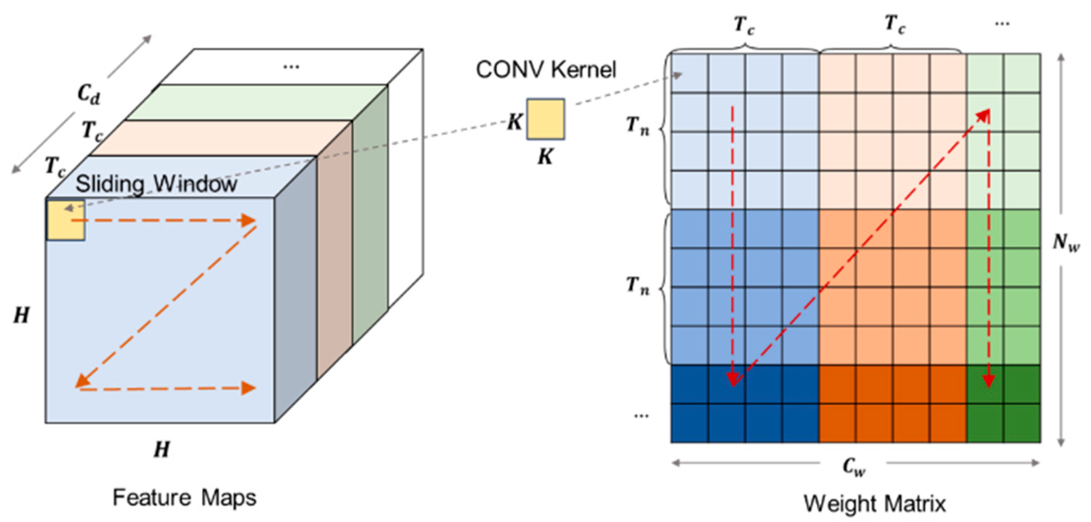
In most embedded hardware implementation, it is unprocurable to store the entire feature maps and weights on the limited on-chip memory. We also use block-based computations and data reuse to eliminate the off-chip accesses; meanwhile, we minimize the on-chip memory occupation. Since the structured filter-wise mask is enforced on the weight matrix, the weight reuse is a relatively straightforward solution to avoid temporary data reaccess from the off-chip memory [46]. Figure 3 illustrates the scheduling scheme. Here we assume that the input feature map has the same height and width, denoted as $H$. Similarly, the height and width of convolutional kernels is denoted as $K$. We adopt the traditional sliding convolution window for convolution. As we can see, the convolution window first slides horizontally across the row, pixel by pixel, then shifts down to the next row and repeats the sliding operation. Supposing stride = 1, with padding for simpler illustration, every kernel will be reused $H\times H$ times, with the convolution window sliding across the feature plane. Meanwhile, there will be K-1 overlapped rows/columns during the sliding process, resulting in the feature data being reused $K\times K$ times. These features provide optimization space for data-path and streaming computation.

As shown in the weight matrix in Figure 3, the convolutional computation is performed in two parallel dimensions: the input channel ($T_c$) and the output channel ($T_n$). Owing to the diversity of kernel masks in FMP among the input channels, the feature elements involved in convolution differ too. Thus, the traditional concept of the convolution block with a size of $K\times K\times T_c$ evolves into independent feature planes (i.e., $K\times K$ pixels) with $T_c$ channels in parallel. Regarding the output channel parallelism, since the filters share the same filter-wise mask, the feature data involved in convolution remains the same among the $T_n$ filters. As a consequence, there are parallel computing channels with an amount of $T_c\times T_n$ running simultaneously, corresponding to the weight block in the same color, shown in Figure 3, which is called a computing unit. Taking data reuse into consideration, firstly, the computing unit moves forwards along the output channel direction, sharing the same feature maps. After shifting $⌈N_w/T_n⌉$ steps, the first $T_c$ input channels are completed. Then, the computing unit comes to the next $T_c$ input channels and repeats the above-mentioned process. The entire input feature map will be traversed after repeating $⌈C_d/T_c⌉$ times, completing the whole convolutional layer.

2.2.2. FMP-Based Convolutional Processing

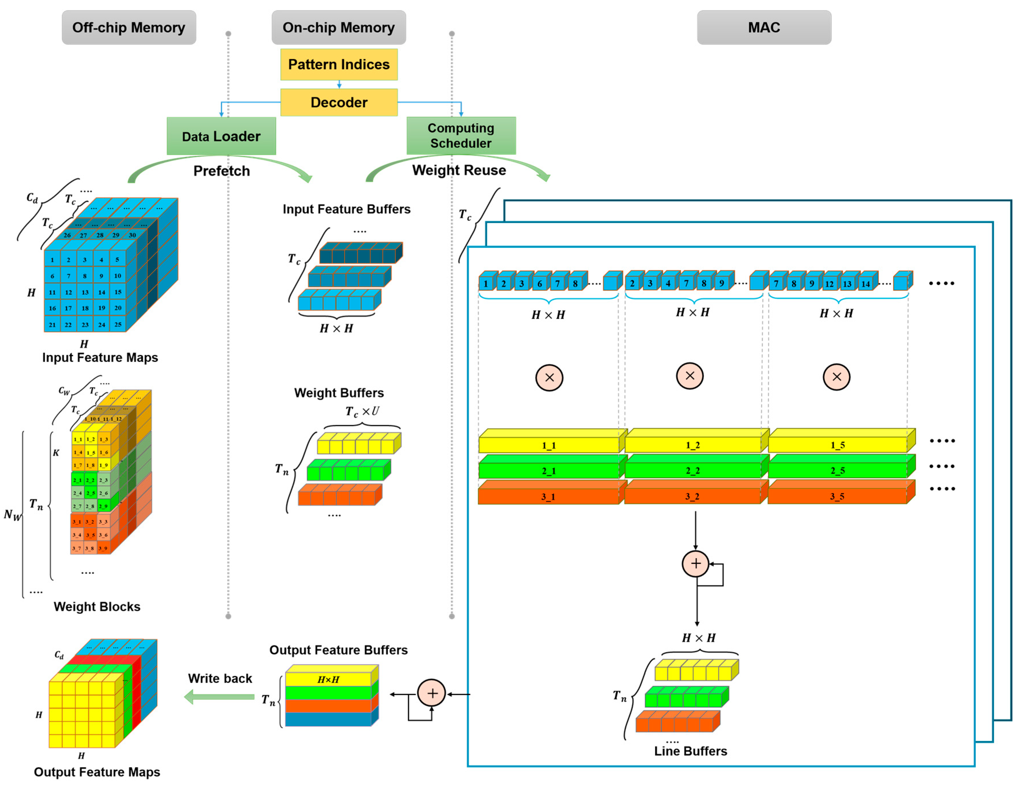
Here, we focus on the convolution computation in a computing unit to demonstrate the convolutional processing, as represented in Figure 4. Although we adopt the traditional concept of a sliding convolution window, we make an advance in substituting the sliding spatial convolution by traversing the input features, where the convolution computation is split into multiplications and accumulations of each weight with its corresponding input features. Each weight element is reused, with $H\times H$ feature elements in one feature plain. Under this transformation, for a certain input channel, only one input feature buffer is needed, and it provides identical input features that can be shared by multiple filters. Unlike the dense network, only the unpruned weights in FMP are involved in computation. Assuming there are $U$ non-zero weights preserved in a kernel, the feature traverse operation repeats U times for every weight in the kernel. The data fetching and convolution computation are controlled by a computing scheduler with the guidance of mask patterns, which are provided by a decoder, according to pattern indices.

The product results of weights and features are cached in a line buffer, first temporarily. With the processing of the following weight and its corresponding feature sequence, the corresponding products are accumulated and rewritten into the line buffer concurrently. Compared with traditional ping-pong buffers, our circular buffers further achieve smaller memory consumption. Corresponding to the parallel computing channels, there are $T_c\times T_n$ line buffers in parallel in total, which store the partial convolution results for each computing channel. Accumulations of the corresponding partial results should be carried out to obtain the final output features, which are cached in output feature buffers. The line buffer size can be set as $H\times H$ at maximum. It is notable that, if the on-chip memory is not large enough for all the line buffers, the number of input features reusing the identical weight can be split into tiles of $T_a$; thus, the line buffer size can be reduced to $T_a$. Under the circumstances, a loop for tiles needs to be brought in to repeat $⌈H\times H/T_a⌉$ times for a whole traverse of the feature map.

In view of the limited on-chip SRAM and off-chip bandwidth, the data access for feature and weight are designed dedicatedly, as illustrated in the left part of Figure 4, which can be explained in conjunction with Figure 3 for better understanding. Supposing feature maps and weights are initialized in off-chip memory, the input feature buffer and weight buffer are established for prefetching. The dual-port block RAMs are used as buffers, which can support reading out for computation and writing in for cache concurrently. Considering that all feature maps participate in computation, the whole feature map with a size of $H\times H$ should be fetched in through burst access. Since the input features data involved in convolution differs among the input channels, $T_c$ feature buffers are established for each input channel, avoiding access conflict. To hide the transmission latency of feature maps, when the computing unit moves to the last one along the output channel, the next feature block containing the next $T_c$ input channel can be prefetched. On this occasion, once the convolution window slides over the feature line, it is no longer in use and can be replaced by the feature line of the next $T_c$ input channel.

In contrast to input feature maps, only the masked weights are necessary for calculation. Considering that all the $T_n$ output channels share the same input features and run concurrently, there should be $T_n$ separate weight buffers for each filter to feed weights synchronously. To simplify the weight buffer design, the weights in one filter are stored in one buffer. Considering $T_c$ computing channels run in parallel and the corresponding weights should be provided through the sole outport of the buffer, we flatten the reading sequence using the idle period during weight reuse. That means computing sequences along the $T_c$ computing channels have delays between each other. The size of one weight buffer is only $T_c\times U$($U$ is the number of non-zero weights in a kernel). As for weight refreshing, weights can also be loaded from external memory, in sync with feature updating.

2.2.3. Overview of Acceleration Architecture

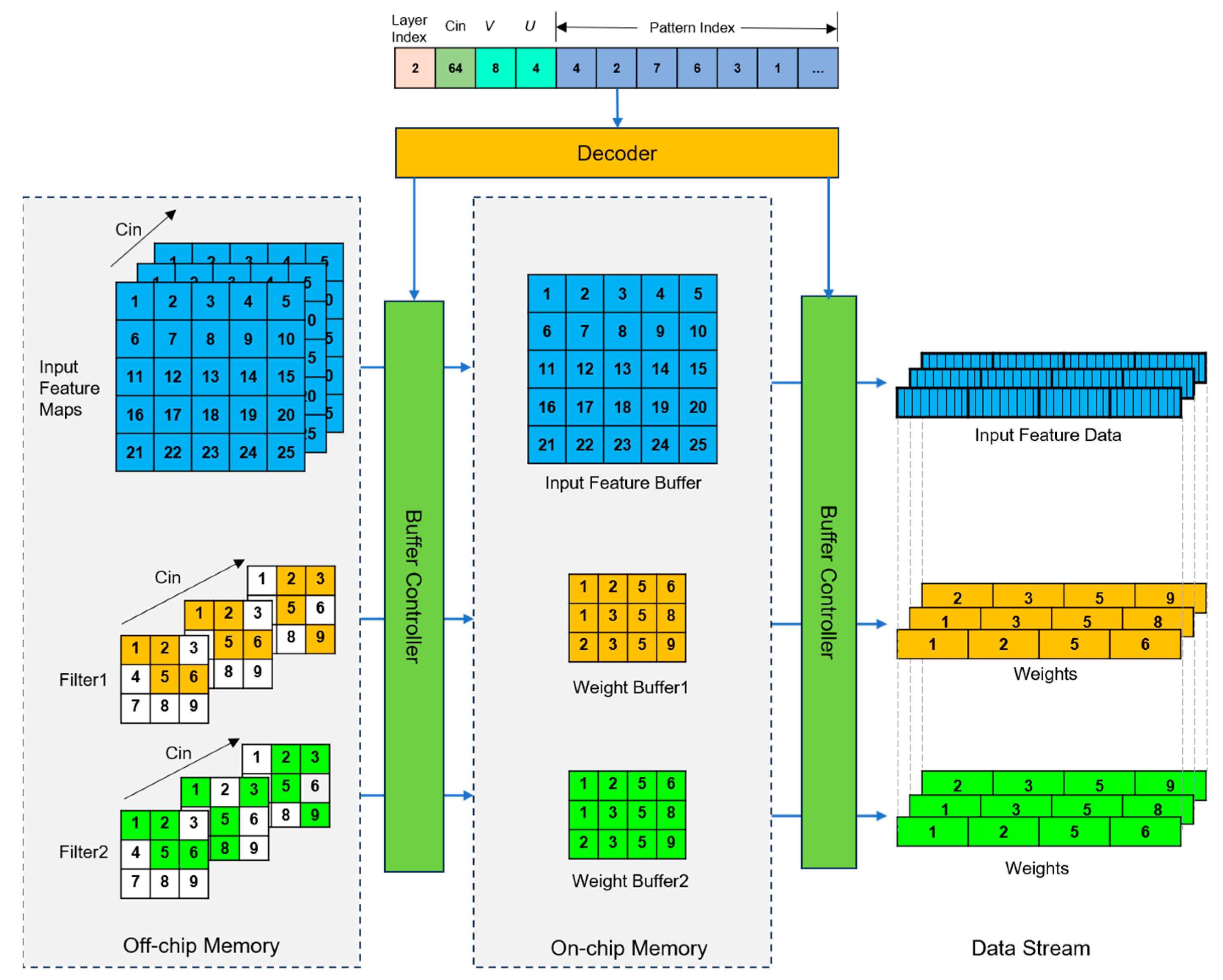
The pattern index and decoder play important roles in guaranteeing regular memory access without an invalid interruption. Figure 5 presents how the decoder guides the data transfer from the off-chip memory to the processing unit. Based on the predefined pattern set, described in Section 2.1, the pattern index array stores the mask index corresponding to input channels for the whole layer. Besides the pattern index, four auxiliary parameters are stored, including the layer index, the number of input channels, the number of patterns $V$ and the number of preserved weights in a kernel $U$. With the full sparse weights initially stored in external memory, the decoder calculates the indices of unpruned weights from pattern index, enabling only preserved weights to be brought into the inner memory. The weights are buffered in a compact and continuous way, in separate buffers for each filter. During this transfer process, the pruned weights are removed, resulting in less memory overhead and continuous weight access for the following computing. The alignment of input data and weights is another significant function. Based on the pattern index, the decoder is capable of calculating the data indices required by the corresponding weights. Thus, unnecessary data access is eliminated, avoiding a pipeline interruption.

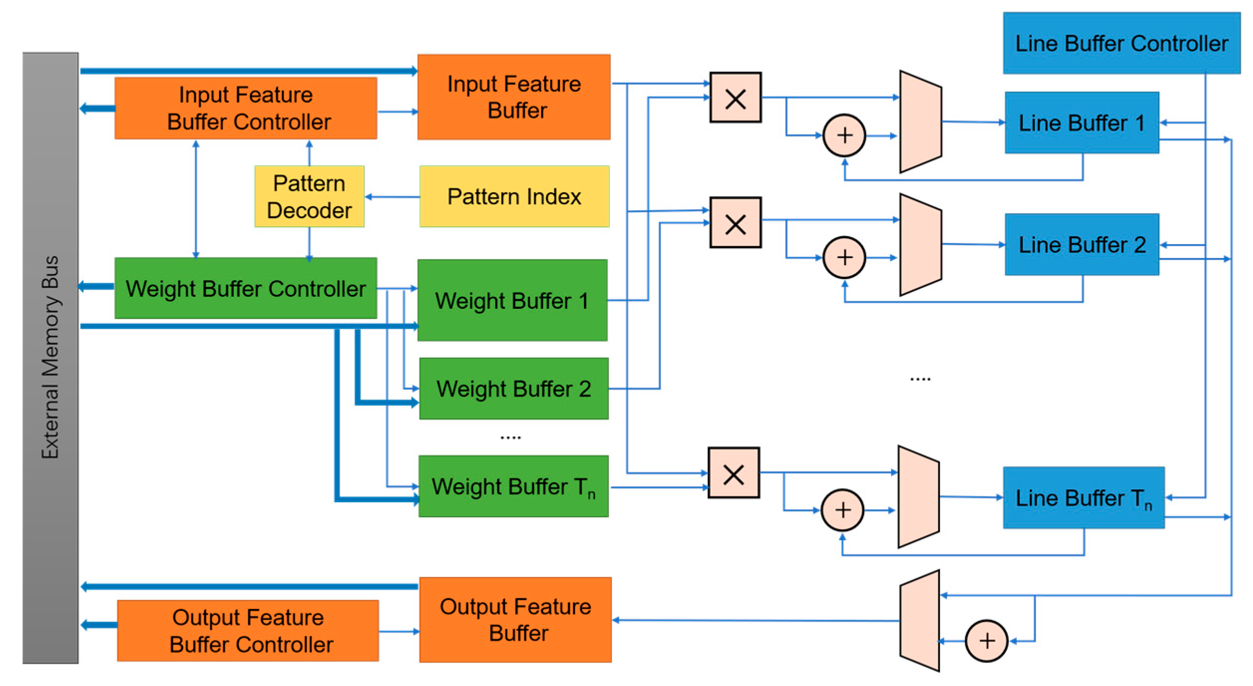
Based on the above discussions, a CNN acceleration architecture based on FMP is proposed and detailed in Figure 6. The major components include buffers, buffer controllers, pattern decoders and MACs. The input feature buffer, weight buffers and line buffers are designed as mentioned above, and are controlled by the corresponding controllers. The input feature buffer controller and weight buffer controller are responsible for transferring the input feature maps and weights into buffers. What is important is that they should read out the input features and weights participating in convolution, following the loading scheme and pattern mask. The pattern decoder translates the pattern index into the pattern mask, guiding the controllers of the input feature buffer and weight buffer. The MAC array conducts multiplications and accumulations in parallel, and the computing is pipelined clock by clock, with scheduling support from data-path optimization. The line buffers support partial product and accumulation cache for each output channel.

For a better understanding, only the parallelism in the output channel direction is represented in Figure 6. In the actual accelerator architecture, the processing is conducted in two parallel dimensions—the input channel ($T_c$) and the output channel ($T_n$)—providing $T_c\times T_n$ parallel computing channels. Each input channel owns a feature buffer, but they can share the same buffer controller, owing to the nearly identical data access logic. There are a total of $T_n$ weight buffers corresponding to each output channel in a computing unit. Each weight buffer is shared by $T_c$ input channels. According to the weight loading scheme, the weight buffers can share the same buffer controller, simplifying the control logic. The line buffers have a total number of $T_c\times T_n$, corresponding to each parallel computing channel. Similarly, the controller for line buffers can be shared due to the identical scheduling. It can be perceived that the buffer controllers can be shared among multiple computing channels to reduce logic overhead, benefiting from the synchronous data access.

3. Results

To validate the proposed filter-wise mask pruning method and acceleration architecture, we first focus on the accuracy performance of VGG-16 and ResNet-50 for object classification and YOLOv5 for object detection; meanwhile, we discuss the details of various pruning configurations. In terms of hardware acceleration, the FPGA implementations with dense models and sparse models are conducted and compared.

3.1. Implementation Settings

Evaluation of proposed FMP on classification networks: We firstly choose the classification networks for evaluation, which have uniform convolution structures and less layers, and are helpful for investigating the efficacy and impact of our proposed pruning method. We adopt two popular network structures: simple VGG-16 (only containing 3 × 3 kernels) and larger-scale ResNet-50 (containing 3 × 3 kernels and 1 × 1 kernels). They are trained on a small-scale dataset, CIFAR10, and a larger-scale dataset, Mini-ImageNet, as presented in

Table 1. Datasets for evaluation.

Datasets	Training Images	Validation Images	Testing Images	Classes
CIFAR-10	45,000	5000	10,000	10
Mini-ImageNet	38,400	9600	12,000	100
Self-established Livestock dataset	344 (8014 Instances)	39 (1751 Instances)	86 (3136 Instances)	3

. Sampled from ImageNet, Mini-ImageNet consists of 60,000 images across 100 classes; it needs fewer training resources and is more friendly for local computers and quick checks. To obtain the benchmarks for each network, we train the models from scratch on PyTorch. The pruning experiments are performed on the pre-trained models. Enforcing the filter-wise mask on the dense model, the sparse training is processed for 45 epochs for CIFAR10 and 36 epochs for Mini-ImageNet. Further, the pruning is conducted with the filter-wise mask, and the sparse model is fine-tuned for 35 epochs for CIFAR10 and 24 epochs for Mini-ImageNet. Other important training parameters are set as follows: stochastic gradient descent (SGD) optimizer with a momentum of 0.9, weight decay of 0.0005, a cosine annealing learning rate policy with an initial learning rate of 0.01. The important training hyperparameters are summarized in

Table 2. Important training hyperparameters.

Models	Sparse Training Epochs	Fine-Tune Epochs	Learning Rate	Weight Decay	Momentum
VGG-16/ResNet-50 On CIFAR10	45	35	CosineAnnealingLR (lr: 0.01)	0.0005	0.9
VGG-16/ResNet-50 On Mini-ImageNet	36	24	CosineAnnealingLR (lr: 0.01)	0.0005	0.9
YOLOv5	60	80	OneCycleLR (lr0: 0.01 lrf: 0.1)	0.0005	0.937

.

Evaluation of proposed FMP on YOLOv5: Further, to fully evaluate the efficacy and applicability of our pruning method, we enforce our method upon the widely used object detection model YOLOv5. Taking into consideration the impact of data redundancy on pruning effectiveness, three relatively lighter models are all estimated, including YOLOv5s, YOLOv5m and YOLOv5l. In this experiment, we use the self-established remote sensing dataset with three types of livestock: cattle, horses and sheep, in which the side length of most objects is between 10 and 30 pixels. The image size is 1024 × 1024 and the whole dataset contains 12,901 livestock instances. First, we train the models for benchmarks from scratch, then the pruning experiments are conducted on the pre-trained models. The sparse training is processed on the dense model for 60 epochs first, after which the pruning is conducted with the filter-wise mask. Then, the sparse model is fine-tuned for 80 epochs to recover accuracy. Other important training parameters are set as follows: a stochastic gradient descent (SGD) optimizer with a momentum of 0.937, weight decay of 0.0005, a one-cycle learning-rate policy with an initial learning rate of 0.01 and a final learning rate of 0.1.

Evaluation of proposed FMP-based accelerator: To demonstrate the hardware performance of the FMP-based acceleration architecture, we implement it in an FPGA platform (Xilinx UltraScale ZU15EG). To simplify the demonstration, the VGG-16 on the Mini-ImageNet dataset is evaluated by its performance and source consumption. The input image’s size is 224 × 224. The model is quantized to 8 bits and is realized in Verilog hardware description language.

3.2. Filter-Wise Mask Pruning on Classification Networks

In this part, we firstly study the performance of our proposed filter-wise mask pruning, with two traditional models: VGG-16 and ResNet-50. After that, comparisons with state-of-the-art pruning methods are conducted. For a fair comparison, only the pruning on CONV layers is discussed, including the convolutional kernels of 3 × 3 and 1 × 1. As discussed above, we enforce the square-shaped mask on 3 × 3 kernels and line-shaped masks on 1 × 1 kernels. Two datasets are adopted for evaluation, including CIFAR-10 with an image size of 32 × 32 and Mini-ImageNet with an image size of 224 × 224.

To dive into a deep analysis of pruning, we elaborate the pruning processes step by step to explore their effects on accuracy performance.

Table 3. Performance comparison of pruning for ResNet-50 on CIFAR10.

Methods	Top-1 Acc (%)	Relative Acc (%)	Params (M)	FLOPs (G)	Compression Rate	Pruning Rate (%)
baseline	94.12	-	20.68	1.19	-	-
SqMk	95.00	+0.88	14.39	0.83	1.44×	30.41
filter-SqMk	94.74	+0.62	14.39	0.83	1.44×	30.41
filter-SqMk + LnMk	94.68	+0.56	9.71	0.56	2.13×	53.04
filter-SqMk + filter-LnMk(FMP)	94.34	+0.22	9.71	0.56	2.13×	53.04
FMP + kernel pruning-A	94.28	+0.16	3.00	0.17	6.88×	85.47
FMP + kernel pruning-B	94.11	−0.01	1.44	0.08	14.37×	93.04
FMP + kernel pruning-L	93.13	−0.99	0.69	0.04	29.89×	96.65

details the accuracy and pruning rate for ResNet-50 on CIFAR10. We first enforce the arbitrary square-shaped mask (termed as SqMk) on 3 × 3 CONV layers in the benchmark model. Given the total number of patterns, $V$ as 8, we set the number of preserved weights in a kernel to be $U=4$, which creates a 1.44× compression rate. Further, we conduct the filter-SqMk, in which all the output channels share an identical filter-wise mask to improve the sparsity regularity. This filter-wise locational constraint of pruning brings in an accuracy drop of 0.26%: from 95.00% to 94.74%. Similarly, we enforce the line-shaped mask (termed as LnMk) on 1 × 1 CONV layers, in which the mask size M is set as 4 and the number of reserved non-zero weights in the mask $N$ is 2. Based on these pattern settings, the compression rate reaches 2.13× and the accuracy drops by 0.06%. After imposing the filter-wise locational constraint on LnMk, the pruning process evolves into our proposed FMP and a +0.22 accuracy improvement still exists, compared with the baseline.

Furthermore, we investigate the fusion with kernel-wise pruning for a potential higher pruning rate. As shown in Table 3, we first perform experiments “FMP + kernel pruning-A” and “FMP + kernel pruning-B”, with the above pattern settings. The fused pruning results show that the kernel pruning further enhances the compression performance, with good integration of FPM. Taking “FMP + kernel pruning-A” as an example, the 3.2× kernel removal only causes an accuracy drop of 0.06%, compared with FMP. In “FMP + kernel pruning-B”, the kernel pruning produces 6.7× compression and the total compression rate reaches 14.37× with little harm to accuracy. To exploit deeper compression space, the layers’ sensitivity to pruning is taken into consideration in “FMP + kernel pruning-L”. For the first three layers, which are more sensitive to pruning, the pruning pattern of FMP is empirically determined as $U=2$ and $N:M=2:4$, while for the rest layers, they are set as $U=1$ and $N:M=1:4$, doubling the removed weights from the first three layers.

Similar results can be achieved for ResNet-50 on Mini-ImageNet, as shown in

Table 4. Performance comparison of pruning for ResNet-50 on Mini-ImageNet.

Methods	Acc (%)		Relative Acc (%)		Params (M)	FLOPs (G)	Compression Rate	Pruning Rate (%)
	Top-1	Top-5	Top-1	Top-5
baseline	79.39	93.06	-	-	20.68	3.75	-	-
SqMk	79.59	93.84	0.20	0.78	14.39	2.61	1.44×	30.40
filter-SqMk	79.38	93.95	−0.01	0.89	14.39	2.61	1.44×	30.40
filter-SqMk + LnMk	78.87	93.64	−0.52	0.58	9.72	1.76	2.13×	53.02
filter-SqMk + filter-LnMk(FMP)	78.75	93.47	−0.64	0.41	9.72	1.76	2.13×	53.02
FMP + kernel pruning-A	78.42	93.33	−0.97	0.27	5.32	0.96	3.89×	74.29
FMP + kernel pruning-L	77.40	93.48	−1.99	0.42	2.79	0.50	7.42×	86.52

. It is obvious that the model exhibits poorer representativeness on the larger-scale dataset, Mini-ImageNet, compared with the small-scale dataset, CIFAR10. This poses a greater challenge when pruning a larger percentage of parameters from the network. With the same pattern settings as mentioned above, it yields an accuracy degradation of 0.64% after FMP. It can be observed that 1 × 1 CONV layers are a little more accuracy-sensitive through the sparsity of the line-shaped mask. For “FMP + kernel pruning-A”, fused with 1.8× kernel pruning, we achieve a total compression rate of 3.89× with an accuracy loss of 0.97%. As discussed above, in the experiment of “FMP + kernel pruning-L”, when the different pruning patterns are applied over layers in FMP, the accuracy takes a non-ideal drop by 1.99%.

Further to this, we compare FMP with other pruning methods for VGG-16 and ResNet-50 on CIFAR10, as shown in

Table 5. Comparison with other compression methods for VGG-16 and ResNet-50 on CIFAR10.

Networks	Methods	Top-1 Acc (%)			Pruning Rate (%)
		Baseline	Pruned	Relative	FLOPs	Para.
VGG-16	PCNN [32]	93.54	93.58	+0.04	66.7	66.7
	KRP [11]	92.76	92.54	−0.22	70.0	70.0
	ITOP [42]	93.29	93.10	−0.19	80.0	80.0
	Ours-FMP	93.42	93.46	+0.04	75.1	75.1
	Ours-FMP + kernel pruning	93.42	93.26	−0.16	79.5	79.5
ResNet-50	Prune it yourself [47]	92.85	92.69	−0.16	34.2	41.5
	MS-KD [48]	95.36	95.12	−0.24	84.1	84.0
	Layer-wise refined pruning [13]	93.60	92.78	−0.82	84.3	86.3
	Ours-FMP	94.12	94.19	+0.07	84.6	84.6
	Ours-FMP + kernel pruning	94.12	94.28	+0.16	85.5	85.5

. On account of the various baselines related to different training conditions, the accuracy loss that is relative to the respective baseline validation accuracy is taken as the comparative factor. In comparison with ResNet-50, VGG-16 has fewer parameters, thus leading to greater challenges to remove fewer formative parameters and pursue a high pruning rate. With the power of FMP, more than 75.1% of parameters are pruned with no accuracy degradation. When combined with kernel pruning, the pruning rate can be enhanced further, but with a decline in accuracy, approaching the ceiling of the tradeoff between compression and accuracy. As for ResNet-50, compared with state-of-the-art, FMP achieves a better performance in accuracy retaining, with a similar pruning rate. Furthermore, the fusion with kernel pruning reinforces the benefits with higher sparsity and accuracy improvement. It can be observed that our method can remarkably compress parameters and reduce FLOPs simultaneously, with no harm to accuracy.

3.3. Evaluation of Pruning Patterns

Further from the filter-wise mask theory work, the important hyperparameters, such as the number of patterns and the number of preserved weights in a mask, should be carefully considered to maintain high accuracy. In this section, we first analyze the pattern features of the most common 3 × 3 kernels. The impact of the number of preserved weights in a kernel, the effect of the central weights and the number of patterns are specifically observed. A subsequent evaluation is made of the parameter N:M in line-shaped pattern masks for 1 × 1 kernels or FC layers. Furthermore, the criteria for pattern selection are discussed.

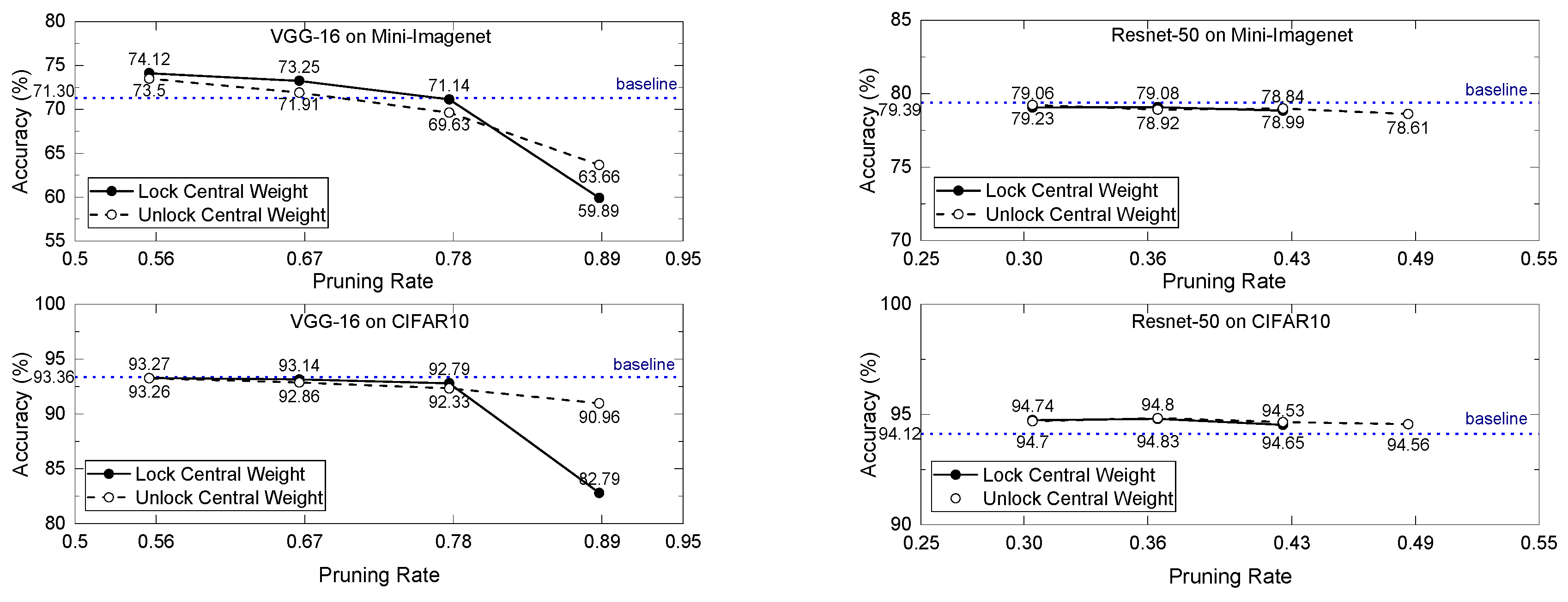
Figure 7 presents the accuracy performance comparison for VGG-16 and ResNet-50 on datasets CIFAR10 and Mini-ImageNet, applying FMP only on 3 × 3 kernels to evaluate the effects of the weight number U and the central weight. Here, the number of candidate patterns, $V$, is set to be eight as an example, and the weight number U is evaluated as one, two, three and four, resulting in pruning rates of 56%, 67%, 78% and 89% in VGG-16. In Resent-50, the pruning rates are 30%, 36%, 43% and 49%, since the parameters in 1 × 1 kernels are not pruned. In the VGG-16 network, we can see a gradual decline in accuracy, along with a reduction in the weight number, U. When the central weight in the mask is consistently kept reserved, the accuracy is a little higher than that of the central weight and is kept or not, depending on its magnitude. The accuracy drops drastically if there is only one weight reserved in the mask. The results for ResNet-50 show that the accuracy discrepancy is quite slight, with the central weight being locked or not. With the count of preserved weights reducing, the accuracy degrades slightly. When there is only one weight reserved in the mask, it can maintain the ideal accuracy, with the largest-magnitude weight remaining. However, if the central weight is kept reserved as the only weight, the accuracy drops by nearly 40%. This is not displayed in the figure for a better view of the detailed variation tendency.

The impact of pattern count selection on accuracy is presented in Figure 8. The weight number in kernel $U$ is set as 1, 2, 3 and 4, and the number of candidate patterns $V$ is evaluated at 2, 4, 6, 8, 16. Obviously, a pattern count of two degrades accuracy unacceptably. In other cases, accuracy performs a certain degree of consistency, and it increases very slightly as the pattern counts increase. The diversity is enlarged at a higher pruning rate, especially when only one weight is reserved.

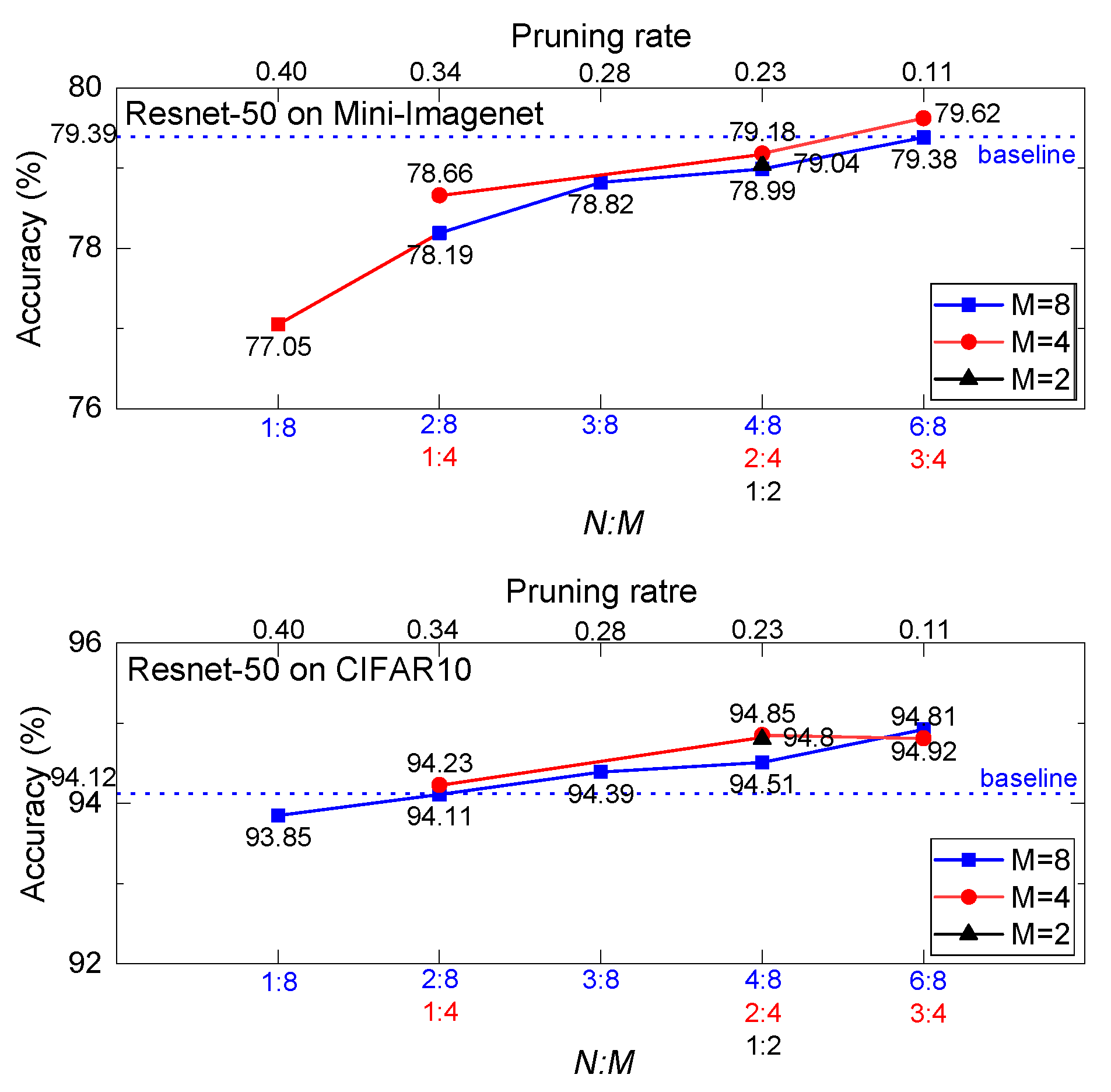
Figure 9 illustrates the performance of pruning conducted on 1 × 1 kernels in the ResNet-50 network, with different N:M masks. It is remarkable that most of the pruning performs better than the baseline on CIFAR10, except $N:M=1:8$. The $1:8$ mask also leads to undesirable accuracy loss on Mini-Imagnet. A noteworthy result is that masks with $M=4$ outperform those with $M=8$ at the same pruning rate.

3.4. Filter-Wise Mask Pruning on YOLOv5

YOLOv5 is still one of the most widely used object detection models in CNNs, especially for deployment in resource-constrained devices, maintaining exceptional accuracy and rapid inference. YOLOv5 adopts the cross stage partial network (CSPNet) to improve the transfer of convolutional neural network feature information effectively. Meanwhile, it also utilizes SPP (spatial pyramid pooling) and PAN (path aggregation network) structures, providing an excellent detection performance and significantly improving the detection speed. One valuable incentive is the elaborated introduction of convolutional kernels with a size of 3 × 3 and 1 × 1. The 1 × 1 kernels in deep networks deal with the large number of input channels with a smaller number of parameters, reducing the computing power consumption concurrently.

We analyze the parameter size in YOLOv5s, YOLOv5m and YOLOv5l, shown in

Table 6. Analysis of parameter size for YOLOv5 models.

Models	Total Params (M)	Params of 3 × 3 Kernels (M)	Params of 1 × 1 Kernels (M)
YOLOv5s	7.01	4.51 (64.4%)	2.49 (35.5%)
YOLOv5m	20.85	14.73 (70.7%)	6.10 (29.3%)
YOLOv5l	46.11	34.34 (74.5%)	11.75 (25.5%)

. The 3 × 3 kernels account for a larger proportion—about 64.4~74.5% in different models—and 1 × 1 kernels take the remaining 35.5~25.5%. This means that the reasonable pruning of both the 3 × 3 kernels and 1 × 1 kernels is essential for the whole model.

In this experiment, we use the self-established remote sensing dataset, containing images of three types of livestock, including cattle, horses and sheep. The images were captured in Hadatu Pasture, Hulunbuir City in China, where there is a large distribution of ordinary livestock. The photographs were taken by a fixed-wing unmanned aerial vehicle (UAV) from an overhead orthographic attitude. The flight altitude was set at about 300 m, while the relative altitude of the flight changed with the rugged terrain. Thus, the images’ spatial resolution was about 3~7 cm, depending on the relative altitude. The side length of most objects is 10–30 pixels. In the dataset, images are split into 1024 × 1024, containing 12,901 livestock instances. The set was randomly divided into training, validation and testing datasets, with a ratio of about 7:1:2. As we can see, this dataset is composed of small objects and densely packed instances: both of which challenge the detectors. Moreover, the similar body shape makes it harder to distinguish animal targets. The dataset is qualified to validate the effectiveness of detection models and our pruning method, and the detection results of pruned YOLOv5s are shown as examples in Figure 10.

For further exploration of the pruning performance, we conduct FMP on the three relative small-scale models of YOLOv5, including YOLOv5s, YOLOv5m and YOLOv5l, and various pruning settings are enforced, as detailed in

Table 7. Performance comparison of pruning for YOLOv5 models.

Models	Methods	mAP (%)	Relative mAP (%)	Params (M)	FLOPs (G)	Compression Rate	Pruning Rate (%)
YOLOv5s	baseline	87.1	-	7.01	16.00	-	-
	FMP	86.5	−0.6	3.26	7.45	2.15×	53.43
YOLOv5m	baseline	88.6	-	20.85	48.20	-	-
	FMP	91.4	+2.8	9.68	22.38	2.15×	53.57
	FMP-L	86.2	−2.4	4.57	10.56	4.56×	78.09
YOLOv5l	baseline	91.6	-	46.11	108.30	-	-
	FMP	93.4	+1.8	21.27	49.97	2.17×	53.86
	FMP-L	89.6	−2.0	5.44	12.77	8.48×	88.21

. Similar to pruning evaluation for VGG-16 and ResNet-50, we also execute FMP on YOLOv5, in which the pruning pattern is determined as $U=4$ and $N:M=2:4$.

With a subtle difference in ratio between 3 × 3 kernels and 1 × 1 kernels in different models, FMP leads to a compression rate of about 2.15×. On account of the larger parameter redundancy with the larger scale of model, the same FMP makes different impacts on accuracy performances. For YOLOv5s, the mAP drops by 0.6%, from 87.1% to 86.5%, while for YOLOv5m and YOLOv5l, the pruning brings in an accuracy enhancement of 2.8% and 1.8%, respectively. Furthermore, to investigate the potential higher pruning rate, we perform FMP-L experiments on YOLOv5m and YOLOv5l. In FMP-L, the layers’ sensitivity to pruning is taken into consideration and the pruning pattern of FMP is empirically determined for layers. For YOLOv5m, when the total amount of parameters reduces to 4.57 M with a compression rate of about 4.56×, the mAP drops to 86.2%, slightly lower than that of pruned YOLOv5s. As for YOLOv5l, the compression rate of 8.48× brings the model size down to 5.44, which is 22.3% lower than the original YOLOv5s. However, its mAP remains at 89.6%, which is 2.5% higher than that of the original YOLOv5s. The experiment results suggest that FMP can identify and remove unimportant model parameters effectively, simultaneously maintaining high detection accuracy.

Further, we compare our filter-wise mask pruning method with other pruning methods for the lighter model: YOLOv5s and YOLOv5m, as presented in

Table 8. Experiment results of various compression methods for YOLOv5.

Models	Methods	mAP (%) Baseline/Pruned	Relative mAP (%)	Params (M)	FLOPs (G)	Compression Rate
YOLOv5s	[49]	96.8/97.5	+0.7	4.45	-	1.57×
	Ours	87.1/88.8	+1.7	4.52	10.32	1.55×
	[50]	91.5/91.0	−0.5	-	18.2	1.95×
	Ours	87.1/86.5	−0.6	3.26	7.45	2.15×
YOLOv5m	[51]	81.6/80.6	−1.0	8.9	23.4	2.38×
	Ours	88.6/90.2	+1.6	8.34	19.27	2.50×

. Here, we still take the accuracy loss relative to the respective baseline validation accuracy as the comparative factor to investigate the impact of compression. For YOLOv5s, the accuracy has a slight increase, with a gentle compression rate of approximately 1.55×, while a mild decrement appears when the compression rate reaches near to 2×. As to YOLOv5m, our method still has an accuracy improvement of 1.6% compared to the baseline, with a compression rate of 2.5×. It can be seen that our method outperforms in accuracy with a similar compression rate.

3.5. Performance of FMP-Based Accelerator

We continue the study on the FMP-based accelerator, implemented on the FPGA platform. To provide a comprehensive demonstration of the accelerator performance, we deploy VGG-16 with Mini-ImageNet for input images. With FMP, we employ square-shaped masks for CONV layers and line-shaped masks for FC layers. For comprehensive comparison, two pruned networks are obtained, with diverse pattern settings—$U=4$, $N:M=2:4$ and $U=2$, $N:M=1:4$—resulting in pruning rates of 55.5% and 77.8%, respectively. The parallelism factor $T_c$ and $T_n$ for the accelerator are both set as 128, meaning that they support 128 input channels and 128 output channels computing concurrently. The FPGA implementation operates at a frequency of 200 MHz.

To further investigate performance enhancement by using FMP, we evaluate the layer-wise throughputs of dense and sparse networks for VGG-16, which are presented in

Table 9. Operation performance of dense network and sparse network with FMP for VGG-16 on Mini-ImageNet.

Layers	Feature Map Size	Dense Network			$\mathit{U}=4,\mathit{N}:\mathit{M}=2:4$			$\mathit{U}=2,\mathit{N}:\mathit{M}=1:4$
		Operations (MOPs)	Execution Time (ms)	Throughput (GOPS)	Operations (MOPs)	Execution Time (ms)	Throughput (GOPS)	Operations (MOPs)	Execution Time (ms)	Throughput (GOPS)
block1_conv1	(224,224,3)	89.92	2.272	39.57	39.96	1.012	39.47	19.98	0.508	39.30
block1_conv2	(224,224,64)	1852.90	6.817	271.79	823.51	3.037	271.12	411.76	1.525	269.92
block2_conv1	(112,112,64)	926.45	1.715	540.11	411.76	0.766	537.47	205.88	0.386	532.79
block2_conv2	(112,112,128)	1851.29	2.287	809.46	822.80	1.021	805.51	411.40	0.515	798.49
block3_conv1	(56,56,128)	925.65	1.155	801.20	411.40	0.517	795.03	205.70	0.262	784.81
block3_conv2	(56,56,256)	1850.49	2.311	800.86	822.44	1.035	794.69	411.22	0.524	784.47
block3_conv3	(56,56,256)	1850.49	2.311	800.86	822.44	1.035	794.69	411.22	0.524	784.47
block4_conv1	(28,28,256)	925.25	1.181	783.76	411.22	0.531	774.54	205.61	0.271	758.48
block4_conv2	(28,28,512)	1850.09	2.361	783.59	822.26	1.062	774.37	411.13	0.542	758.32
block4_conv3	(28,28,512)	1850.09	2.361	783.59	822.26	1.062	774.37	411.13	0.542	758.32
block5_conv1	(14,14,512)	462.52	0.616	750.75	205.57	0.280	733.95	102.78	0.146	705.54
block5_conv2	(14,14,512)	462.52	0.616	750.75	205.57	0.280	733.95	102.78	0.146	705.54
block5_conv3	(14,14,512)	462.52	0.616	750.75	205.57	0.280	733.95	102.78	0.146	705.54
FC1	(4096)	102.76	0.157	655.36	51.38	0.078	655.36	25.69	0.039	655.36
FC2	(4096)	16.78	0.026	655.36	8.39	0.013	655.36	4.19	0.006	655.36
FC3	(4096)	0.41	0.001	512.00	0.20	0.000	512.00	0.10	0.000	512.00
Total	-	15,480.13	26.803	577.55	6886.72	12.010	573.36	3443.36	6.084	565.94
Speedup	-	-			2.23×			4.4×
Compression Rate	-	-			2.25×			4.5×

. Taking the convolution block1 as an example, with three input channels and 64 output channels in layer block1_conv1and 64 input channels and 128 output channels in layer block1_conv2, the parallel computing channels are far from being fully utilized, leading to a lower throughput. With the increasing channels, the later convolution blocks achieve higher resource utilization and computation capability. The maximum throughput reaches 809.46 GOPS at layer block2_conv2. The throughput is also affected by the size of the feature map because of the data access time; that is why it degrades slightly at deeper layers. Compared with dense networks, the sparse networks achieve a conspicuous execution time reduction, nearly in proportion to the pruning rate. Consequently, the maximum and average throughputs can maintain a high performance, close to that of a dense network. It can be observed that the FMP-based architecture can efficiently leverage the strength of our FMP method, fully converting the weight pruning to computation reduction.

The resource utilization for the dense and sparse networks of VGG-16 implemented in FPGA are listed in

Table 10. FPGA resource consumption of dense network and sparse network. Parallelism factor $T_c=T_n=128$.

Sources	Available	Dense Network	$\mathit{U}=4,\mathit{N}:\mathit{M}=2:4$	$\mathit{U}=2,\mathit{N}:\mathit{M}=1:4$
LUTs	341.3 K	279.0 K (81.76%)	276.6 K (81.05%)	276.1 K (80.90%)
FFs	682.6 K	279.4 K (40.94%)	279.0 K (40.88%)	278.9 K (40.86%)
LUTRAMs	184.3 K	2304 (1.25%)	2304 (1.25%)	2304 (1.25%%)
BRAMs (36 Kb)	744	416 (55.91%)	416 (55.91%)	416 (55.91%)
DSPs	3528	785 (22.25%)	785 (22.25%)	785 (22.25%)

. In most cases, the DSP resource is likely to be the strictest constraint during hardware implementation, since the Vivado Synthesis tool tends to map multiplications to DSPs, leading to a shortage of DSPs, especially for the full-precision networks. Herein, the weights and activations are quantized to an 8-bit fixed point and the low-precision multiplication can be implemented by using look up tables (LUTs), no longer limited by DSP resources. The implementation enjoys this benefit to support the parallelism channels up to 128, in which the LUTs utilization reaches about 80% and the DSPs keep a low occupancy. As discussed in Section 2.2, the on-chip memory overhead also profits from FMP-based architecture, only taking up half of the total memory. The overhead difference among the dense and sparse networks is quite small and is determined by the FMP-based architecture and the parallelism channels. In conjunction with Table 9, the sparse convolution computing takes full advantage of computing resources, and the weight reduction directly scales down the execution time, due to the optimization of data-path and computation streaming.

Furthermore, we make comparisons to prior studies concerning VGG-16 on FPGA platforms, as shown in

Table 11. Comparison with other FPGA implementations of VGG-16.

	[53] (X. Lian, 2019)	[52] (Q. Yi, 2021)	[54] (D. Kim, 2023)	[55] (C. Yang, 2024)	Ours
FPGA	XC7VX690T	XC7Z045	XCVU9P	XCVU9P	XCZU15EG
Frequency (MHz)	200	200	200	430	200
DSPs	1027 (29%)	900 (98%)	2286 (33%)	576 (8%)	785 (22%)
LUTs	231.8 K (54%)	118.0 K (54%)	814 K (69%)	93 K (8%)	279.0 K (82%)
FFs	141 K (16%)	148.6 K (34%)	795 K (34%)	NA	279.4 K (41%)
BRAMs	913 (62%)	403 (74%)	1663 (77%)	336 (16%)	416 (56%)
Throughput (GOPS)	760.83	706	402	711	809.46
Performance Efficiency (GOPS/DSP)	0.74	0.78	0.18	1.23	1.03
Power (W)	9.18	7.2	NA	37.6	8.4
Power Efficiency (GOPS/W)	82.88	98.06	NA	18.9	96.36

. The detailed implementation information, such as platform, working frequency, overheads and performances, is taken into consideration. It can be observed that our accelerator outperforms in both throughput and performance efficiency. Compared with existing works, our design achieves an improvement of throughput of more than 6.4%. With the comprehensive analysis of resource utilization on different FPGA platforms, we employ performance efficiency (the number of arithmetic operations equivalent to per DSP) for a fair comparison. The result shows that the performance efficiency increases by 32%, compared with [52]. These improvements mainly come from the optimized memory access and calculation pipeline, which gives a guarantee of good workload balance and resource efficiency.From a comprehensive perspective, our proposed architecture achieves a remarkable performance, with a desirable applicability for both dense and sparse networks.

4. Discussion

Real-time processing in remote sensing has been evolving rapidly, driven by advancements in remote sensing detectors, computing technology and algorithm and hardware upgrades. It has emerged as a crucial requirement for emergency response, dynamic monitoring, agricultural investigation, and so on. Benefiting from the collaborative breakthroughs among algorithms, hardware and scenarios, remote sensing processing is transitioning from “post hoc analysis” to “in situ intervention”. The Japanese ALOS-2 satellite [56] provides the capability of generating surface deformation maps within 15 min through on-board SAR data processing in real time. The Φsat-2 satellite of the European Space Agency achieves on-board cloud detection, ship detection and classification and image compression with six artificial intelligence applications, providing a smarter and more efficient way to monitor our Earth. Therefore, the edge intelligence is playing a more and more essential role in future remote sensing applications.

When it comes to hardware implementation and deployment on edge devices, the harsh resource restriction, whether on on-orbit satellites or UAVs, imposes stringent limitations on the size and complexity of CNN models and the power and reliability of the equipped devices. Although most of the existing CNN-based methods are prototyped on power-hungry GPU platforms [8,9,10], FPGAs are a better alternative for on-satellite/on-UAVs deployment, due to their flexible customization, low power, high performance and stronger ionizing-radiation tolerance [57]. Thus, we focus our attention upon how to build an accelerator to maximize the efficiency of FPGA.

Different from works on algorithms’ improvement for object classification and detection, our work focuses on relatively more general technology: the software–hardware codesign. In this paper, we propose a novel filter-wise mask pruning (FMP) method to compress the CNN models, which aims to maintain model accuracy and achieve satisfactory acceleration simultaneously. Further, we build an acceleration architecture with the strategy of efficient streaming computing, calculation parallelism and memory access, to fully convert the model compression to execution speedup effectively.

As we all know, due to the significant redundancy of the parameterization of CNNs, weight pruning achieves remarkable success in reducing model size. In the past few years, plenty of prior works on unstructured pruning [58,59] have been studied intensively, which can remove arbitrary redundant weights inside a network. However, one insurmountable drawback of these unstructured pruning methods is the irregular sparsity of the weight matrix, which relies on dedicated hardware or libraries’ support, and hardly achieves an ideal inference speedup in general-purpose hardware implementation. In contrast to unstructured pruning, structured pruning removes the entirety of the kernels/channels/filters, according to certain metrics, and produces regular compressed models, which are more favorable in hardware acceleration. Since the original convolution structure is preserved, there is no need for support from dedicated hardware/libraries. Unfortunately, structured sparsity is often accompanied by accuracy degradation. Though the gap between the general unstructured pruning and the coarse-grained structured pruning is observed, and some methods based on pattern pruning are motivated, the weight distribution is still irregular, demanding extra compiler optimization. Meanwhile, the indices overhead are only relatively reduced, but the data throughput is not relieved.

In pursuit of a better compromise between hardware efficiency and accuracy, we propose the filter-wise mask pruning (FMP) method, which enforces extra filter-wise structural constraints on pattern-based pruning. The newly introduced structural constraint on filter dimensions leads to more regularity, generating more hardware-friendly and performant models.

We firstly choose the classification networks for evaluation, which have uniform convolution structures and less layers, and are helpful to investigate the efficacy and impact of our proposed pruning method. Compared with the state-of-the-art, FMP achieves a better performance in accuracy retention, with a similar pruning rate. Furthermore, the fusion with kernel pruning reinforces the benefits, with a higher sparsity and accuracy improvement. It can be observed that our method can remarkably compress parameters and reduce FLOPs simultaneously, with no harm to accuracy.

Further, to fully evaluate the efficacy and applicability of our pruning method, we enforce our method on the widely used object detection model YOLOv5, which is still one of the most widely used object detection models in CNNs, especially for deploying within resource-constrained devices. Here, we use our self-established remote sensing dataset, based on photography taken by a fixed-wing UAV. The pruned YOLOv5s achieve a pruning rate of 53.43%, with a slight accuracy degradation of 0.6%. Compared with other pruning methods for the lighter models, our method outperforms in accuracy with a similar compression rate.

To promote the proposed pruning method for reference acceleration in edge devices, we further build the FMP-based acceleration architecture, with strategies including efficient streaming computing, calculation parallelism and memory access optimization. We also implement the FMP-based acceleration architecture on an FPGA platform, achieving the maximum throughput, up to 809.46 MOPS. When the network is pruned with compression rates of 2.25× and 4.5×, it can achieve a speedup of 2.23× and 4.4×, respectively, exhibiting promising execution acceleration. It is noticeable that the architecture is not only dedicated to our pruning method but is also adaptive to dense convolution.

Although the evaluation of FPGA proves our method to be an effective solution, it is also promising for other edge devices, such as embedded GPUs: another comprehensively used processor on mobile platforms. However, the implementations on GPUs heavily rely on dedicated software libraries, e.g., CUBLAS, or hardware resources, e.g., Tensor Core, which are more sophisticated in dense computation acceleration. It becomes challenging to leverage these tools to accelerate the fine-grained sparsity in our method. Therefore, we are making efforts to break this limitation and are making our method well-generalized to GPUs in near future.

5. Conclusions

We introduce a novel pruning pattern of filter-wise masks to pursue a better tradeoff between accuracy and execution performance. By enforcing extra filter-wise structural constraints on pattern-based pruning, we enhance fine-grained sparsity with more regularity. This improvement brings benefits for calculation parallelism and memory access in hardware accelerators, thus leading to an excellent workload balance and throughput. Finally, we evaluate the accuracy performance for both simple classification networks and complex detection networks. For VGG-16 and ResNet-50, the pruning rates can be 75.1% and 84.6%, with a small accuracy promotion by 0.04% and 0.07%, respectively. As for YOLOv5s, it achieves a pruning rate of 53.43% with a slight accuracy degradation of 0.6%, while for the larger-scale models, YOLOv5m and YOLOv5l, the pruning rates can be promoted to 78.09% and 88.21%, with accuracy reductions of 2.4% and 2.0%, respectively. In deploying the acceleration architecture in FPGA, the sparse network achieves a speedup of 2.23× and 4.4×, with compression rates of 2.25× and 4.5×, respectively. The experiment results demonstrate that our approach qualifies hardware accelerators as being adaptive to pruning improvements.

References

1. Yang, G.; Lei, J.; Xie, W.; Fang, Z.; Li, Y.; Wang, J. Algorithm/Hardware Codesign for Real-Time On-Satellite CNN-Based Ship Detection in SAR Imagery. IEEE Trans. Geosci. Remote Sens. 2022, 60, 1–18. [Google Scholar] [CrossRef]
2. Gong, H.; Mu, T.; Li, Q.; Dai, H.; Li, C.; He, Z.; Wang, W.; Han, F.; Tuniyazi, A.; Li, H.; et al. Swin-Transformer-Enabled YOLOv5 with Attention Mechanism for Small Object Detection on Satellite Images. Remote Sens. 2022, 14, 2861. [Google Scholar] [CrossRef]
3. Han, D.; Lee, S.B.; Song, M.; Cho, J.S. Change Detection in Unmanned Aerial Vehicle Images for Progress Monitoring of Road Construction. Buildings 2021, 11, 150. [Google Scholar] [CrossRef]
4. Vanhoy, G.; Lichtman, M.; Hoare, R.R.; Brevik, C. Rapid Prototyping Framework for Intelligent Arrays with Heterogeneous Computing. In Proceedings of the 2022 IEEE International Symposium on Phased Array Systems & Technology (PAST), Waltham, MA, USA, 11–14 October 2022; pp. 1–6. [Google Scholar] [CrossRef]
5. Li, W.; Liu, J.; Mei, H. Lightweight convolutional neural network for aircraft small target real-time detection in Airport videos in complex scenes. Sci. Rep. 2022, 12, 14474. [Google Scholar] [CrossRef] [PubMed] [PubMed Central]
6. Wu, Z.; Zhang, C.; Gu, X.; Duporge, I.; Hughey, L.F.; Stabach, J.A.; Skidmore, A.K.; Hopcraft, J.G.C.; Lee, S.J.; Atkinsonet, P.M.; et al. Deep learning enables satellite-based monitoring of large populations of terrestrial mammals across heterogeneous landscape. Nat. Commun. 2023, 14, 3072. [Google Scholar] [CrossRef]
7. Golcarenarenji, G.; Martinez-Alpiste, I.; Wang, Q.; Alcaraz-Calero, J.M. Efficient Real-Time Human Detection Using Unmanned Aerial Vehicles Optical Imagery. Int. J. Remote Sens. 2021, 42, 2440–2462. [Google Scholar] [CrossRef]
8. Sun, Y.; Zheng, L.; Wang, Q.; Ye, X.; Huang, Y.; Yao, P. Accelerating Sparse Deep Neural Network Inference Using GPU Tensor Cores. In Proceedings of the 2022 IEEE High Performance Extreme Computing Conference (HPEC), Waltham, MA, USA, 19–23 September 2022; pp. 1–7. [Google Scholar] [CrossRef]
9. Lin, D.-L.; Huang, T.-W. Accelerating Large Sparse Neural Network Inference Using GPU Task Graph Parallelism. IEEE Trans. Parallel Distrib. Syst. 2022, 33, 3041–3052. [Google Scholar] [CrossRef]
10. Li, Z.; Yuan, G.; Niu, W.; Zhao, P.; Li, Y.; Cai, Y. NPAS: A Compiler-aware Framework of Unified Network Pruning and Architecture Search for Beyond Real-Time Mobile Acceleration. In Proceedings of the 2021 IEEE/CVF Conference on Computer Vision and Pattern Recognition (CVPR), Nashville, TN, USA, 20–25 June 2021; pp. 14250–14261. [Google Scholar] [CrossRef]
11. Sui, X.; Lv, Q.; Zhi, L.; Zhu, B.; Yang, Y.; Zhang, Y.; Tan, Z. A Hardware-Friendly High-Precision CNN Pruning Method and Its FPGA Implementation. Sensors 2023, 23, 824. [Google Scholar] [CrossRef]
12. Zhang, J.; Cheng, L.; Li, Y.; He, G.; Xu, N. A Low-Latency FPGA Implementation for Real-Time Object Detection. In Proceedings of the 2021 IEEE International Symposium on Circuits and Systems (ISCAS), Daegu, Republic of Korea, 22–28 May 2021; pp. 1–5. [Google Scholar] [CrossRef]
13. Li, H.; Yue, X.; Wang, Z.; Chai, Z.; Wang, W.; Hiroyuki, T.; Lin, M. Optimizing the Deep Neural Networks by Layer-Wise Refined Pruning and the Acceleration on FPGA. Comput. Intell. Neurosci. 2022, 2022, 8039281. [Google Scholar] [CrossRef]
14. Eckert, C.; Wang, X.; Wang, J.; Subramaniyan, A.; Iyer, R.; Sylvester, D.; Blaauw, D.; Das, R. Neural cache: Bitserial in-cache acceleration of deep neural networks. In Proceedings of the 45th Annual International Symposium on Computer Architecture (ISCA), Los Angeles, CA, USA, 1–6 June 2018; IEEE Press: New York, NY, USA, 2018; pp. 383–396. [Google Scholar]
15. Hegde, K.; Yu, J.; Agrawal, R.; Yan, M.; Pellauer, M.; Fletcher, C.W. Ucnn: Exploiting computational reuse in deep neural networks via weight repetition. In Proceedings of the 45th Annual International Symposium on Computer Architecture (ISCA), Los Angeles, CA, USA, 1–6 June 2018; IEEE Press: New York, NY, USA, 2018; pp. 674–687. [Google Scholar]
16. Jain, A.; Phanishayee, A.; Mars, J.; Tang, L.; Pekhimenko, G. Gist: Efcient data encoding for deep neural network training. In Proceedings of the 2018 ACM/IEEE 45th Annual International Symposium on Computer Architecture (ISCA), Los Angeles, CA, USA, 1–6 June 2018; IEEE: New York, NY, USA, 2018; pp. 776–789. [Google Scholar]
17. Huang, K.; Li, B.; Chen, S.; Claesen, L.; Xi, W.; Chen, J. Structured Term Pruning for Computational Efficient Neural Networks Inference. IEEE Trans. Comput.-Aided Des. Integr. Circuits Syst. 2023, 42, 190–203. [Google Scholar] [CrossRef]
18. Chen, S.; Huang, K.; Xiong, D.; Li, B.; Claesen, L. Fine-Grained Channel Pruning for Deep Residual Neural Networks. In Artificial Neural Networks and Machine Learning—ICANN 2020. ICANN 2020; Farkaš, I., Masulli, P., Wermter, S., Eds.; Lecture Notes in Computer Science; Springer: Cham, Switzerland, 2020; Volume 12397. [Google Scholar] [CrossRef]
19. Rhu, M.; O’Connor, M.; Chatterjee, N.; Pool, J.; Kwon, Y.; Keckler, S. Compressing DMA Engine: Leveraging Activation Sparsity for Training Deep Neural Networks. In Proceedings of the 2018 IEEE International Symposium on High Performance Computer Architecture (HPCA), Vienna, Austria, 24–28 February 2018; IEEE: New York, NY, USA, 2018; pp. 331–344. [Google Scholar]
20. Akhlaghi, V.; Yazdanbakhsh, A.; Samadi, K.; Gupta, R.K.; Esmaeilzadeh, H. Snapea: Predictive early activation for reducing computation in deep convolutional neural networks. In Proceedings of the 2018 ACM/IEEE 45th Annual International Symposium on Computer Architecture (ISCA), Los Angeles, CA, USA, 2–6 June 2018; IEEE: New York, NY, USA, 2018; pp. 662–673. [Google Scholar]
21. Li, C.; Wang, G.; Wang, B.; Ling, X.; Li, Z.; Chang, X. Dynamic Slimmable Network. In Proceedings of the IEEE Conference on Computer Vision and Pattern Recognition, CVPR, Virtual, 19–25 June 2021; IEEE: New York, NY, USA, 2021; pp. 8607–8617. [Google Scholar]
22. Dai, X.; Yin, H.; Jha, N.K. NeST: A Neural Network Synthesis Tool Based on a Grow-and-Prune Paradigm. IEEE Trans. Comput. 2019, 68, 1487–1497. [Google Scholar] [CrossRef]
23. He, Y.; Zhang, X.; Sun, J. Channel Pruning for Accelerating Very Deep Neural Networks. In Proceedings of the Computer Vision (ICCV), Venice, Italy, 22–29 October 2017; IEEE: New York, NY, USA, 2017; pp. 1398–1406. [Google Scholar]
24. Guo, Y.; Yao, A.; Chen, Y. Dynamic network surgery for efficient dnns. In Advances in Neural Information Processing Systems; Curran Associates: New York, NY, USA, 2016; pp. 1379–1387. [Google Scholar]
25. Han, S.; Pool, J.; Tran, J.; Dally, W. Learning both weights and connections for efficient neural network. In Advances in Neural Information Processing Systems; MIT Press: Cambridge, UK, 2015; pp. 1135–1143. [Google Scholar]
26. Mao, H.; Han, S.; Pool, J.; Li, W.; Liu, X.; Wang, Y.; Dally, J.W. Exploring the granularity of sparsity in convolutional neural networks. In Proceedings of the 2017 IEEE Conference on Computer Vision and Pattern Recognition Workshops, CVPR Workshops 2017, Honolulu, HI, USA, 21–26 July 2017; pp. 1927–1934. [Google Scholar]
27. Buluç, A.; Fineman, J.T.; Frigo, M.; Gilbert, J.R.; Leiserson, C.E. Parallel sparse matrix-vector and matrix-transpose-vector multiplication using compressed sparse blocks. In Proceedings of the Twenty-First Annual Symposium on Parallelism in Algorithms and Architectures, Calgary, AB, Canada, 11–13 August 2009; ACM: New York, NY, USA, 2009; pp. 233–244. [Google Scholar]
28. Anwar, S.; Hwang, K.; Sung, W. Structured pruning of deep convolutional neural networks. ACM J. Emerg. Technol. Comput. Syst. 2017, 13, 1–18. [Google Scholar] [CrossRef]
29. Renda, A.; Frankle, J.; Carbin, M. Comparing rewinding and fine-tuning in neural network pruning. In Proceedings of the International Conference on Learning Representation (ICLR), Simien Mountains, Ethiopia, 30 April 2020. [Google Scholar]
30. Ma, X.; Guo, F.M.; Niu, W.; Lin, X.; Tang, J.; Ma, K.; Ren, B.; Wang, Y. PCONV: The Missing but Desirable Sparsity in DNN Weight Pruning for Real-time Execution on Mobile Devices. arXiv 2019, arXiv:1909.05073. [Google Scholar] [CrossRef]
31. Niu, W.; Ma, X.; Lin, S.; Wang, S.; Qian, X.; Lin, X.; Wang, Y.; Ren, B. PatDNN: Achieving Real-Time DNN Execution on Mobile Devices with Pattern-based Weight Pruning. In Proceedings of the Twenty-Fifth International Conference on Architectural Support for Programming Languages and Operating Systems, Lausanne, Switzerland, 16–20 March 2020; pp. 907–922. [Google Scholar]
32. Tan, Z.; Song, J.; Ma, X.; Tan, S.; Chen, H.; Miao, Y. PCNN: Pattern-based Fine-Grained Regular Pruning Towards Optimizing CNN Accelerators. In Proceedings of the 2020 57th ACM/IEEE Design Automation Conference (DAC), San Francisco, CA, USA, 20–24 July 2020; pp. 1–6. [Google Scholar] [CrossRef]
33. Xu, X.; Zhang, X.; Zhang, T. Lite-YOLOv5: A lightweight deep learning detector for on-board ship detection in large-scene sentinel-1 AR images. Remote Sens. 2022, 14, 1018. [Google Scholar] [CrossRef]
34. Chen, B.; Zhang, R.; Tan, Y.; Li, P. LE-YOLO: A Novel Lightweight Object Detection Method. In Proceedings of the 2023 3rd International Conference on Computer Science, Electronic Information Engineering and Intelligent Control Technology (CEI), Wuhan, China, 15–17 December 2023; pp. 477–480. [Google Scholar] [CrossRef]
35. Ma, X.; Ji, K.; Xiong, B.; Zhang, L.; Feng, S.; Kuang, G. Light-YOLOv4: An edge-device oriented target detection method for remote sensing images. IEEE J. Sel. Top. Appl. Earth Obs. Remote Sens. 2021, 14, 10808–10820. [Google Scholar] [CrossRef]
36. Yu, H.; Lee, S.; Yeo, B.; Han, J.; Park, E.; Pack, S. Towards a Lightweight Object Detection through Model Pruning Approaches. In Proceedings of the 2023 14th International Conference on Information and Communication Technology Convergence (ICTC), Jeju Island, Republic of Korea, 11–13 October 2023; pp. 875–880. [Google Scholar] [CrossRef]
37. Zhou, A.; Ma, Y.; Zhu, J.; Liu, J.; Zhang, Z.; Yuan, K.; Sun, W.; Li, H. Learning N:M Fine-grained Structured Sparse Neural Networks from Scratch. arXiv 2021, arXiv:2102.04010. [Google Scholar]
38. Mishra, A.K.; Latorre, J.A.; Pool, J.; Stosic, D.; Stosic, D.; Venkatesh, G.; Yu, C.; Icikevicius, P. Accelerating Sparse Deep Neural Networks. arXiv 2021, arXiv:2104.08378. [Google Scholar] [CrossRef]
39. Molchanov, P.; Tyree, S.; Karras, T.; Aila, T.; Kautz, J. Pruning convolutional neural networks for resource efficient transfer learning. arXiv 2016, arXiv:1611.06440. [Google Scholar]
40. Lee, N.; Ajanthan, T.; Torr, P. SNIP: Single-Shot Networkpruning Based on Connection Sensitivity. In Proceedings of the International Conference on Learning Representations, New Orleans, LA, USA, 6–9 May 2019. [Google Scholar]
41. Molchanov, P.; Mallya, A.; Tyree, S.; Frosio, I.; Kautz, J. Importance estimation for neural network pruning. In Proceedings of the IEEE Conference on Computer Vision and Pattern Recognition, Long Beach, CA, USA, 16–20 June 2019; pp. 11264–11272. [Google Scholar]
42. Mocanu, D.C.; Lu, Y.; Pechenizkiy, M. Do We Actually Need Dense Over-Parameterization? In-Time Over-Parameterization in Sparse Training. In Proceedings of the International Conference on Machine Learning, Online, 18–24 July 2021. [Google Scholar]
43. Liu, Z.; Li, J.; Shen, Z.; Huang, G.; Yan, S.; Zhang, C. Learning efficient convolutional networks through network slimming. In Proceedings of the IEEE International Conference on Computer Vision, Venice, Italy, 22–29 October 2017; pp. 2736–2744. [Google Scholar]
44. Yang, T.-J.; Chen, Y.-H.; Sze, V. Designing energy-efficient convolutional neural networks using energy-aware pruning. In Proceedings of the IEEE Conference on Computer Vision and Pattern Recognition, Honolulu, HI, USA, 21–26 July 2017; pp. 6071–6079. [Google Scholar]
45. Yu, J.; Lukefahr, A.; Palframan, D.; Dasika, G.; Das, R.; Mahlke, S. Scalpel: Customizing dnn pruning to the underlying hardware parallelism. In Proceedings of the Computer Architecture (ISCA), 2017 ACM/IEEE 44th Annual International Symposium, Toronto, ON, Canada, 24–28 June 2017; IEEE: New York, NY, USA, 2017; pp. 548–560. [Google Scholar]
46. Sun, F.; Wang, C.; Gong, L.; Xu, C.; Zhang, Y.; Lu, Y. A high-performance accelerator for large-scale convolutional neural networks. In Proceedings of the 2017 IEEE International Symposium on Parallel and Distributed Processing with Applications and 2017 IEEE International Conference on Ubiquitous Computing and Communications (ISPA/IUCC), Guangzhou, China, 12–15 December 2017; pp. 622–629. [Google Scholar]
47. Yan, Z.; Xing, P.; Wang, Y.; Tian, Y. Prune it yourself: Automated pruning by multiple level sensitivity. In Proceedings of the IEEE Conference on Multimedia Information Processing and Retrieval (MIPR), Shenzhen, China, 6–8 August 2020; pp. 73–78. [Google Scholar]
48. Chen, R.; Yuan, S.; Wang, S.; Li, Z.; Xing, M.; Feng, Z. Model selection—Knowledge distillation framework for model compression. In Proceedings of the IEEE Symposium Series on Computational Intelligence (SSCI), Orlando, FL, USA, 5–7 December 2021. [Google Scholar]
49. Chen, C.; Gan, Y.; Han, Z.; Gao, H.; Li, A. An Improved YOLOv5 Detection Algorithm with Pruning and OpenVINO Quantization. In Proceedings of the 2023 China Automation Congress (CAC), Chongqing, China, 17–19 November 2023; pp. 4691–4696. [Google Scholar] [CrossRef]
50. Sun, X.; Liu, Z.; Zhao, J.; Zhu, J.; Zheng, Z.; Ji, Z. Research on Multi-target Detection of Lightweight Substation Based on YOLOv5. In Proceedings of the 2024 5th International Conference on Computer Vision, Image and Deep Learning (CVIDL), Zhuhai, China, 19–21 April 2024; pp. 1337–1341. [Google Scholar] [CrossRef]
51. Wang, P.; Yu, Z.; Zhu, Z. Channel Pruning-Based Lightweight YOLOv5 for Pedestrian Object Detection. In Proceedings of the 2023 5th International Symposium on Robotics & Intelligent Manufacturing Technology (ISRIMT), Changzhou, China, 22–24 September 2023; pp. 229–232. [Google Scholar] [CrossRef]
52. Yi, Q.; Sun, H.; Fujita, M. FPGA Based Accelerator for Neural Networks Computation with Flexible Pipelining. arXiv 2021, arXiv:2112.15443v1. [Google Scholar] [CrossRef]
53. Lian, X.; Liu, Z.; Song, Z.; Dai, J.; Zhou, W.; Ji, X. High-performance FPGAbased CNN accelerator with block-floating-point arithmetic. IEEE Trans. Very Large Scale Integr. Syst. 2019, 27, 1874–1885. [Google Scholar] [CrossRef]
54. Kim, D.; Jeong, S.; Kim, J.-Y. Agamotto: A performance optimization framework for CNN accelerator with row stationary dataflow. IEEE Trans. Circuits Syst. I Regul. Pap. 2023, 70, 2487–2496. [Google Scholar] [CrossRef]
55. Yang, C.; Yang, Y.; Meng, Y.; Huo, K.; Xiang, S.; Wang, J. Flexible and efficient convolutional acceleration on unified hardware using the two-stage splitting method and layer-adaptive allocation of 1-D/2-D winograd units. IEEE Trans. Comput.-Aided Des. Integr. Circuits Syst. 2024, 43, 919–932. [Google Scholar] [CrossRef]
56. Natsuaki, R.; Ohki, M.; Nagai, H.; Motohka, T.; Tadono, T.; Shimada, M.; Suzuki, S. Performance of ALOS-2 PALSAR-2 for disaster response. In Proceedings of the 2017 IEEE International Geoscience and Remote Sensing Symposium (IGARSS), Fort Worth, TX, USA, 23–28 July 2017; pp. 2434–2437. [Google Scholar] [CrossRef]
57. Lei, J.; Yang, G.; Xie, W.; Li, Y.; Jia, X. A low-complexity hyperspectral anomaly detection algorithm and its FPGA implementation. IEEE J. Sel. Top. Appl. Earth Obs. Remote Sens. 2020, 14, 907–921. [Google Scholar] [CrossRef]
58. Liu, Z.; Xu, J.; Peng, X.; Xiong, R. Frequencydomain dynamic pruning for convolutional neural networks. Adv. Neural Inf. Process. Syst. 2018, 31, 1049–1059. [Google Scholar]
59. Frankle, J.; Carbin, M. The lottery ticket hypothesis: Finding sparse, trainable neural networks. In Proceedings of the International Conference on Learning Representations (ICLR), New Orleans, LA, USA, 6–9 May 2019. [Google Scholar]
Figure 1. The visualization of the existing pruning method and our proposed method.
Remotesensing 17 03582 g001
Figure 2. Overview of filter-wise mask pruning and acceleration. For the square-shaped 3 × 3 mask, 4 weights are preserved in a kernel. For the line-shaped mask, 2 weights are preserved in every 4 consecutive weights.
Remotesensing 17 03582 g002
Figure 3. Scheduling scheme for parallel convolutional computation.
Remotesensing 17 03582 g003
Figure 4. Parallel strategy of data-path and convolutional computation for FMP.
Remotesensing 17 03582 g004
Figure 5. Scheme for data storage and transfer.
Remotesensing 17 03582 g005
Figure 6. Overview of the proposed acceleration architecture.
Remotesensing 17 03582 g006
Figure 7. Performance comparison of FMP for VGG-16 (left) and ResNet-50 (right). The pruning is only conducted on 3 × 3 kernels with different number of preserved weights in a kernel mask.
Remotesensing 17 03582 g007
Figure 8. Impact of the number of patterns across diverse models and datasets.
Remotesensing 17 03582 g008
Figure 9. Performance of FMP for ResNet-50 with N:M mask on 1 × 1 kernels.
Remotesensing 17 03582 g009
Figure 10. Livestock object detection results of pruned YOLOv5s. (a) Cattle. (b) Sheep. (c) Horses.
Remotesensing 17 03582 g010