Abstract
This paper addresses the problem of target localization in a distributed waveform diverse array radar system, exploiting the technique of sparse reconstruction. At the configuration stage, the distributed radar system consists of two individual Frequency Diverse Array Multiple-Input Multiple-Output (FDA-MIMO) radars and one single Element-Pulse Coding MIMO (EPC-MIMO) radar. To obtain the angle and incremental range (i.e., the range offset between the sampling point and actual position within the range bin) of the targets in each local radar, two sparse reconstruction-based algorithms, including the grid-based Iterative Adaptive Approach (IAA) and gridless Atomic Norm Minimization (ANM) algorithms, are implemented. Furthermore, multiple sets of local statistics are fused at the fusion center, where a Weighted Least Squares (WLS) method is performed to localize targets. At the analysis stage, the estimation performance of the proposed methods, encompassing both IAA and ANM algorithms, is evaluated in contrast to the Cramér–Rao Bound (CRB). Numerical results and parametric studies are provided to demonstrate the effectiveness of the proposed sparse reconstruction methods for target localization in the distributed waveform diverse array system.
1. Introduction
Target localization is an indispensable application that has raised significant attention within the radar scientific community [1,2,3]. However, the localization of weak targets has become a significant challenge in practical applications [4,5]. Typically, weak targets exhibit characteristics such as a low Radar Cross Section (RCS), meaning they are easily buried in the background of noise [6,7]. These characteristics make these targets difficult to detect accurately, which in turn has a negative impact on the overall performance of radar systems [8]. Traditional phased array radars are widely used for target localization, where high-precision target detection can be achieved by forming a beam in the intended direction using multiple antenna elements [9,10,11]. In [10], a novel adaptive sampling interval algorithm for multi-target tracking is introduced. Moreover, a joint target assignment and resource optimization strategy for multi-target tracking with the phased array radar is proposed [11]. However, for weak targets, the detection performance is reduced due to the low Signal-to-Noise Ratio (SNR) of weak targets [12,13,14]. To tackle the problem, a viable solution is to employ the distributed radar system by jointly operating multiple spatially separated radars, which leverages the spatial diversity to enhance target detection and localization performances for weak targets [15,16].
Currently, the localization methods with distributed radar systems are mainly divided into two categories, including direct positioning methods [17,18] and indirect positioning methods [19,20]. In particular, the former involves data acquisition in each individual station and data fusion in the fusion center without any a priori processing. In this regard, the fusion center aggregates the received data from all stations and performs unified signal processing to obtain the target’s information. Such a method enjoys the advantages of high-precision estimation. However, it results in a huge computational load [21,22]. In contrast, with the latter method, the data is processed in each individual station to obtain target parameters, including angle, incremental range, and range ambiguity index. Then, the information related to all stations is transmitted to the fusion center, where further processing is carried out to localize the target [23,24]. Hence, the processing efficiency is significantly improved compared with the direct processing methods. In this respect, a localization method for the target using distributed radar systems is presented in [25], in which a closed-form solution of target position is derived via a two-stage Weighted Least Squares (WLS) framework. Furthermore, an iterative-based target position refinement process is designed to alleviate the off-grid problem caused by spatial discretization using a significantly higher computational efficiency and a lower data communication burden compared with the direct positioning methods [26].
Recently, the concept of Frequency Diverse Array (FDA) has garnered widespread attention. In this context, a small frequency increment is introduced between adjacent transmit elements [27,28,29]. Furthermore, by integrating FDA with Multiple-Input Multiple-Output (MIMO) technology, it is possible to obtain the range–angle-dependent beampattern after digital mixing and separating the transmitted waveforms. Therefore, the additional Degrees of Freedom (DOFs) in the range dimension can be acquired, which enables the simultaneous estimation of target’s range and angle [30]. In this context, the incremental range, which denotes the range offset between the sampling and actual positions within the range bin, can be obtained [31]. To achieve more precise range estimation, three approximated maximum likelihood techniques are designed in [32]. Furthermore, by extending the FDA-MIMO into multiple pulses, an equivalent coding coefficient is introduced across the transmit elements and pulses, which leads to another alternative framework, i.e., the Element-Pulse Coding MIMO (EPC-MIMO) radar. In this respect, the equivalent pointing directions corresponding to different pulses in the EPC-MIMO radar are introduced, enabling the separation of range ambiguity [33]. Specifically, an enhanced parameter estimation approach is developed to obtain the angle and range region number index (also termed as the number of delayed pulses) of the target [34]. Moreover, a reweighted atomic norm minimization-based approach is developed to separate range-ambiguous clutter by leveraging transmit spatial frequencies from different range ambiguity regions [35].
Following the guidelines, by combining the waveform-diverse array radars and the distributed system, a potential detection advantage for weak targets can be obtained by exploiting both the spatial and waveform diversities [36]. In this paper, the target localization in a distributed waveform diverse array radar system consisting of two individual FDA-MIMO radars and a single EPC-MIMO radar is configured, exploiting the technique of sparse reconstruction [37,38]. The main contributions of this paper can be summarized as follows:
- (i)
- At the configuration stage, the distributed waveform diverse array radar system is formed by three local stations [39,40,41], including two individual FDA-MIMO radars and a single EPC-MIMO radar. Notably, both the FDA-MIMO and EPC-MIMO radars are configured in a colocated MIMO architecture. Specially, the incremental range and angle parameters are measured by the FDA-MIMO radar. In the meanwhile, the range ambiguity index and angle parameters are acquired by the EPC-MIMO radar.
- (ii)
- The Iterative Adaptive Approach (IAA) [42,43,44] and the Atomic Norm Minimization (ANM) [45,46,47] algorithms are employed at FDA-MIMO radar stations for parameter estimation. Simultaneously, the angle and range ambiguity index are acquired by the EPC-MIMO radar through the Coordinate Descent Multiple-Signal Classification (CD-MUSIC) method. Furthermore, based on the single-station estimation results, the WLS method is used by the fusion center to localize targets [48];
- (iii)
- At the analysis phase, both the Cramér–Rao Bounds (CRBs) for the FDA-MIMO and EPC-MIMO radars are derived. In addition, the Root Mean Square Errors (RMSEs) versus the SNRs are provided to verify the effectiveness of the methods. Furthermore, a comprehensive localization error analysis is carried out.
The organization of the paper proceeds as follows. Section 2 presents the signal model of the distributed waveform diverse radar system. In Section 3, multi-dimensional parameter estimation based on sparse reconstruction theory is studied. To demonstrate the efficacy of the proposed method, numerical results are provided in Section 4. Finally, Section 5 summarizes the article and explores potential directions for future research.
Notations: Boldface is utilized for vectors (in lowercase), where the n-th component is denoted as , and for matrices (in uppercase), where the -th column is represented as . A matrix can be defined by the columns (i.e., ). The transpose and the conjugate transpose operators are denoted by the symbols and , respectively. , and are, respectively, the sets of N-dimensional vectors of complex numbers, N-dimensional vectors real numbers, and complex matrices. ⊙, ⊗ and ∘ represent the Hadamard (elementwise) product, the Kronecker product and the Khatir–Rao product, respectively. The letter j represents the imaginary unit (i.e., ). The refers to extracting the main diagonal elements of into a column vector, and represents an column vector of ones. The is the infimum operator. The determinant of the matrix is indicated with . For any , denotes its Euclidian norm. The returns the l-th diagonal elements of .
2. Signal Model of Distributed Waveform Diverse Array Radars
Consider a distributed radar system in Cartesian coordinates. The system is comprised of three local radar stations, including two FDA-MIMO radars and one EPC-MIMO radar, as illustrated in Figure 1. Notably, both the FDA-MIMO and EPC-MIMO radars are configured in a colocated MIMO arrangement using uniform linear arrays, which comprises M transmit and N receive antenna elements [49]. The spacing between the antenna elements is set at half-wavelength, with the first element designated as the reference.
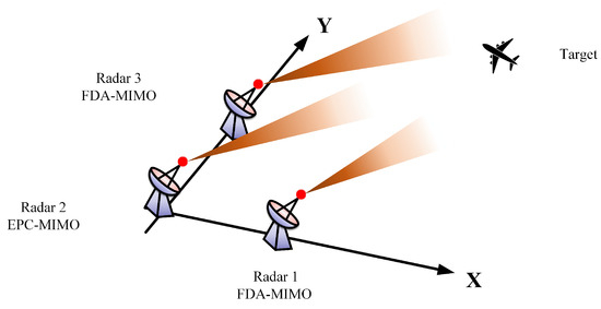
Figure 1.
Distributed waveform diverse radars scenario.
2.1. FDA-MIMO Radar
The signal model for a specific FDA-MIMO radar is presented in this section. By employing a sequential frequency increment, which is termed , to each element of the transmit array, the carrier frequency assigned to the m-th element is thus expressed
where denotes the reference carrier. Subsequently, the transmit signal of the m-th transmit element is
where E denotes the transmitted signal’s power, represents the radar pulse duration, and is the baseband waveform assumed to satisfy the orthogonal condition, formulated as follows
where denotes an arbitrary time delay.
Considering a point-like target in the far field with range and angle , the signal transmitted from the m-th element of the transmit array and received by the target can be described as follows
where and c denotes the speed of light.
To proceed, the signal received by the n-th element can be described as
where is the complex echo amplitude, denotes the envelope time delay, and this approximation underscores the narrowband assumptions, implying that .
After undergoing the preprocessing steps, the signal can be characterized as follows
where .
Then, the useful samples received from the cell under test can be aggregated to construct an dimensional vector
where
- with the incremental delay w.r.t. the sampling time associated with the target range cell;
- represents the angle-dependent receive steering vector;
- with the transmit waveforms correlation matrix, of which the -th entry of , , and the angle-dependent transmit steering vector;
- denotes the range-dependent steering vector.
2.2. EPC-MIMO Radar
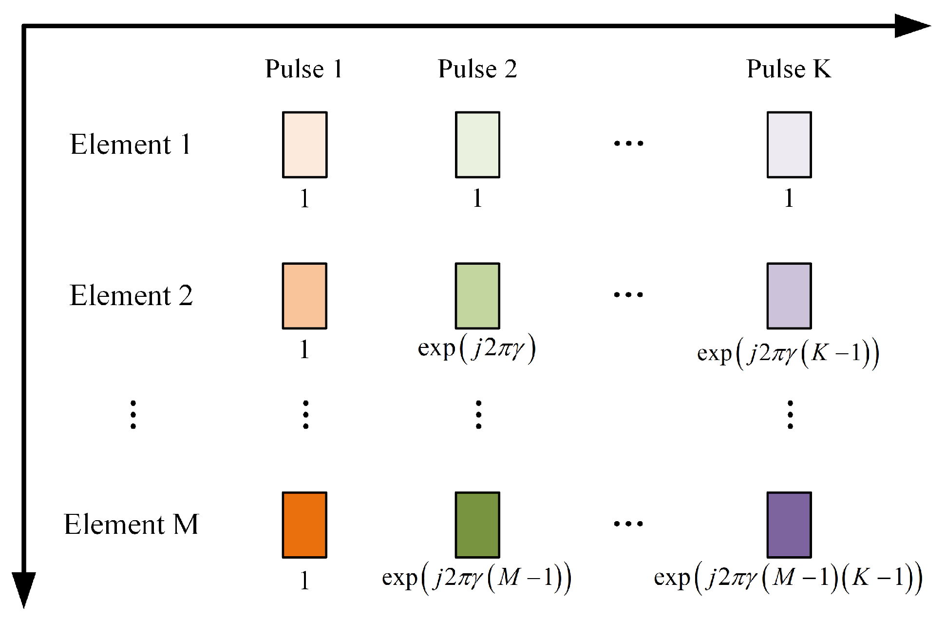
In this section, the signal model for the EPC-MIMO radar is established, with its two-dimensional coding schematic depicted as in Figure 2.

Figure 2.
Element-pulse two-dimensional coding diagram.
Given K pulses transmitted within each coherent processing interval, the signal emanating from the m-th element during the k-th pulse can be described as
where , B represents the bandwidth and is the EPC phase factor, i.e.,
where denotes a user-defined coding parameter. Consequently, the EPC vector corresponding to the k-th pulse can be expressed as
Assume that a far-field target is located at . The echo signal received by the n-th element, originating from the m-th element during the k-th pulse, can be formulated as
where signifies the complex amplitude and denotes the number of delayed pulses.
Subsequently, the signal undergoes mixing and matched filtering by employing the m-th filter defined as , which yields
Hence, the signals corresponding to all transmit pulses and receive elements are formulated in the following expression
Therefore, the decoding procedure is carried out as follows
where .
Thus, the echo signal gathered from the k-th pulses can be expressed as
where
- denotes the transmit steering vector with ;
- , with the amplitude coefficient of the target.
3. Target Localization Based on Sparse Reconstruction
3.1. Target Localization with a Distributed Radar System
In this subsection, the WLS method is applied at the fusion center to localize targets, utilizing statistical data gathered from the local stations. Notably, the number of radar stations is set to V. A specific localization scenario is considered where the SNR of the target is different across different local radar stations. Therefore, fusing these local statistics with equal weights for localization is impractical and could lead to significant localization inaccuracies.
To address this issue, a linear transformation is first applied to the SNRs obtained at each station, thus the v-th station is represented as
Subsequently, the weights are further refined based on the SNRs as
where T is the temperature coefficient.
Afterwards, multiple sets of parameters received from all local FDA-MIMO/EPC-MIMO radar stations are integrated by the fusion center of the distributed radar system. Therefore, the target’s observation position is represented as and can be formulated accordingly
and
where the positions of distributed radars are denoted as , represents the angle of the target measured by the v-th radar station, and similarly denotes the range information.
The WLS method is applied to achieve target localization, and the objective function can be expressed as
where represents the target position to be solved, denotes the observation matrix, is the error matrix, and represents the weight matrix. Therefore, the target location to be solved is
3.2. Iterative Adaptive Approach
In this subsection, the IAA algorithm is employed for parameter estimation problems in FDA-MIMO radar [50,51,52]. Now, letting (satisfying , can be further expressed as
where .
Assume that L targets are located in the far field of space. The received signal can be represented as
where denotes the steering vector matrix of targets, represents a zero-mean complex circularly symmetric Gaussian random vector, i.e., the Gaussian white noise, and .
The two-dimensional space formed by incremental range and angle domains is divided into Q grids. Notice that is ensured for the sparsity of signals in the range domain. Therefore, the incremental range–angle corresponding to each grid is expressed as
The received signal, subsequent to sparse processing, can be expressed as
where .
Assume that is a dimensional diagonal matrix where its diagonal elements correspond to the power values of each grid point, of which the q-th value is
Then, the noise covariance matrix is defined, and it can be represented as follows at the q-th grid point
where denotes the covariance matrix of the received signal.
Therefore, the parameter estimation results are obtained through a WLS-based IAA algorithm as follows
where represents the complex amplitude of the signal at the q-th grid point during the k-th pulse.
The Equation (28) can be further expressed as
In order to activate the IAA, an initialization of is required, with an initial value assigned to , namely
The above process is repeated iteratively until a specific condition is met or a preset number of iterations is reached. Subsequently, the signal power at the grid points is given. Thus, the parameter estimation of the target is achieved. The procedures of the mentioned IAA algorithm for the FDA-MIMO radar are summarized in Algorithm 1.
| Algorithm 1 FDA-IAA |
3.3. Atomic Norm Minimization Approach
The ANM algorithm is introduced in this subsection [39,40,53]. As can be seen from Equation (23), the incremental range information and angle information are coupled within the steering vector , which may lead to ambiguity in the parameter estimation results. Therefore, a decoupling model for the received signal in the k-th pulse is presented to separate the angle and incremental range information, which is written as
where denotes the amplitude and phase of the l-th target at the k-th pulse.
Then, define as the set formed by extracting the non-redundant elements from . Hence, the Equation (31) can be rewritten as
Next, the extracting matrix is constructed with . Notably, the -th element in the m-th row of is one, and other elements are zero. Therefore, the Equation (32) can be re-expressed as
where , , and .
Then, the received signals for K pulses can be presented as
where , , and . Thus, the decoupling model for angle-incremental range is obtained as in Equation (34).
The following defines a 2D atomic set as the target’s angle and incremental range
According to Equation (34), a new matrix is defined as follows [54]
where , , and . Thus, matrix can be considered as a linear combination of L atoms in the atomic set ℑ.
According to compressed sensing theory, the sparsity of the received signal is characterized by its norm, defined as
Notably, the problem of norm minimization is NP-hard, and it is difficult to obtain an exact solution. Thus, the norm is usually used as a substitute in practice, represented as follows
Then, according to [55,56], by minimizing and convex relaxation, Equation (38) can be transformed into the following Semi-Definite Programming (SDP) problem
where with , and and represent auxiliary variables. The denotes the transformation of into a Hermitian matrix, which can be written as
where (for ) is formulated as
Considering the noise background, the objective function in Equation (39) is further modified as
where represents the regularized parameter.
By solving Equation (42), it yields the . Subsequently, the estimated values of the target’s incremental range and angle can be obtained by applying the decomposition theorem to [57]. The procedures of the mentioned ANM algorithm for the FDA-MIMO radar are summarized in Algorithm 2.
| Algorithm 2 FDA-ANM |
3.4. Coordinate Descent Multiple Signal Classification Approach
In this subsection, the CD-MUSIC algorithm is employed for the parameter estimation (i.e., the angle and range ambiguity index) in the EPC-MIMO radar [58,59]. The MUSIC algorithm is leveraged by exploiting the eigenstructure of the signal covariance matrix, which is obtained through snapshots data, namely
Notably, the noise subspace matrix is constructed from the eigenvectors corresponding to the smallest eigenvalues. In particular, the matrix is obtained through the eigenvalue decomposition of the sample covariance matrix . Consequently, the spatial spectrum of the MUSIC algorithm is derived as follows
where denotes the transceive steering vector.
The procedures of the mentioned CD-MUSIC algorithm for the EPC-MIMO radar are summarized in Algorithm 3. Notice that the exit condition is , with a controllable small value. Therefore, the angle and range ambiguity index can be separately obtained by searching for the maximum value of P.
| Algorithm 3 EPC-CD-MUSIC |
|
3.5. CRBs for the FDA-MIMO Radar and EPC-MIMO Radar
In this subsection, the CRBs for the FDA-MIMO radar and the EPC-MIMO radar are developed to characterize the statistical efficiency of the proposed methods.
3.5.1. FDA-MIMO Radar
Let us first define three auxiliary vectors, i.e., , , and , with the positive-definite covariance matrix of the noise. In this context, the real-valued vector , which encapsulates the unknown parameters , , , , is introduced as
Subsequently, the CRBs for the angle and incremental range are derived under the assumption that remains unknown. Hence, the CRBs for the unknown parameters are provided by the diagonal elements of , where the Fisher Information Matrix (FIM) can be presented as
Therefore, the FIM can be expressed as
where
- ;
- ;
- ;
- .
Hence, the can be obtained as the inverse of , i.e.,
where is expressed as
3.5.2. EPC-MIMO Radar
Similarly, three auxiliary vectors are defined, i.e., , , and . In this context, the real-valued vector , which encapsulates the unknown parameters , and , , is introduced as
Subsequently, the CRBs for angle and range ambiguity index are derived under the assumption that remains unknown. Hence, the CRBs for the unknown parameters are provided by the diagonal elements of , where the FIM can be presented as
Therefore, the FIM can be expressed as
where
- ;
- ;
- ;
- .
Hence, the can be obtained as the inverse of , i.e.,
where is expressed as
4. Numerical Results
In this section, numerical examples are presented to evaluate the localization performance of the proposed methods. The performance of the methods is evaluated across various SNR values, which are defined according to [60], as
Monte Carlo trials are executed to assess the performance. Moreover, the RMSEs in terms of angle and range are calculated as follows
and
where denotes the number of independent experiments and , , and represent the estimated angle, incremental range, and range ambiguity index in the i-th independent experiment, respectively. Furthermore, the simulation parameters involved the analyzed case are provided in Table 1.

Table 1.
Simulation parameters of the distributed waveform-diverse array radars.
4.1. Performance Analysis of the Sparse Reconstruction Approach
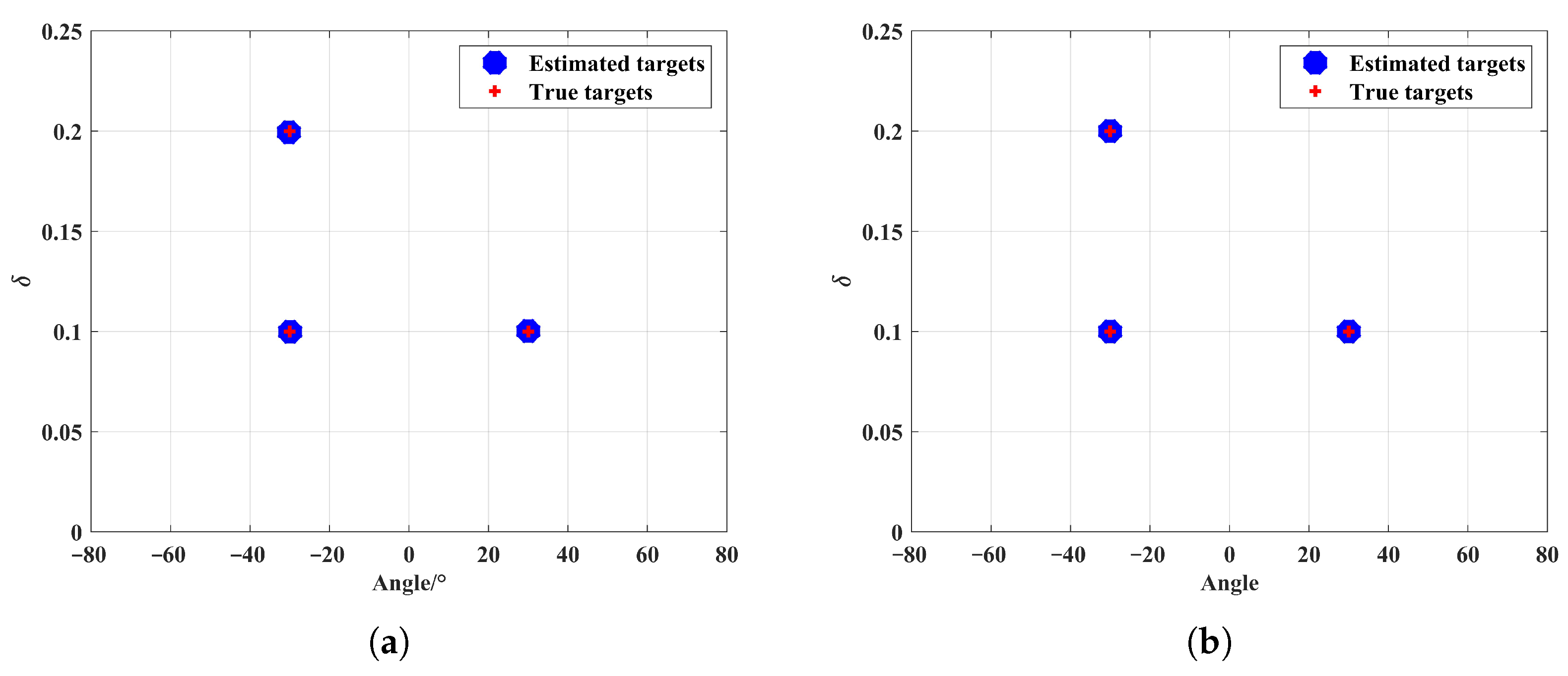
In this subsection, numerical examples are presented to evaluate the effectiveness of the proposed methods to estimate the target’s incremental range and angle of arrival within the framework of an FDA-MIMO radar system. Specifically, the angle grid (−90°, 90°) containing 181 sample points is employed by the IAA algorithm. Meanwhile, the incremental range grid consisting of 501 sample points is also utilized in the following case. The actual target is set as . In this experiment, the effectiveness of the proposed methods is studied, considering two extra targets with and . It can be observed that target shares the same angle with one target and the same incremental range with another.
The estimation outcomes of the two algorithms are provided in Figure 3. Apparently, the estimation results for the targets perfectly coincide with the actual positions. Additionally, targets located at the same angle but with different incremental ranges, or those with the same incremental range but different angles, can be clearly separated. The outcomes validate the effectiveness of the two proposed algorithms.
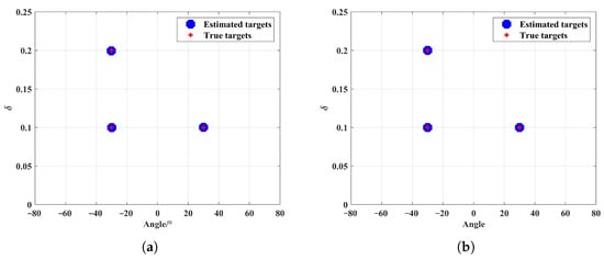
Figure 3.
Increment range–angle estimation result with the proposed method: (a) IAA; (b) ANM.
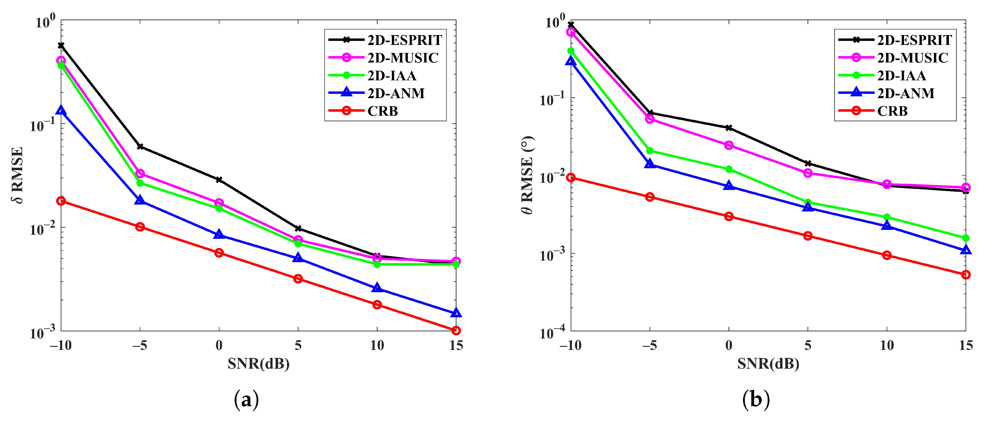
To further shed light on performance of the different methods, Figure 4 illustrates the RMSE versus SNR w.r.t the incremental range–angle estimation. It is evident that as the SNR increases, the estimation accuracy of both algorithms undergoes a notable improvement, ultimately achieving satisfactory performance at relatively high SNR levels. Moreover, when the SNR attains a sufficiently high level within the context of the given scenario, the performance of both algorithms converges relatively closely to the benchmark established by the CRB. Notably, when compared with the parameter estimation algorithms based on 2D subspaces in [58,59], the algorithms discussed in this context demonstrate significant advantages in parameter estimation performance. Furthermore, as evidenced by the numerical results in Figure 4, the estimation performance of the 2D-ANM at SNR = 15 dB demonstrates improvements of at least 1.6 dB, 8.1 dB, and 7.7 dB compared to the 2D-IAA, 2D-MUSIC, and 2D-ESPRIT algorithms, respectively.
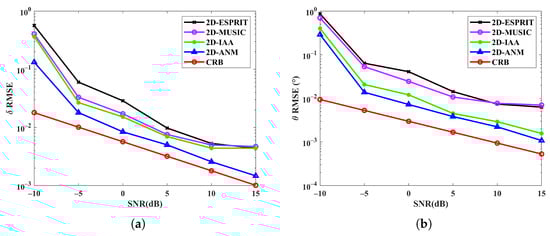
Figure 4.
RMSE versus SNR for increment range–angle estimation: (a) Increment range; (b) Angle.
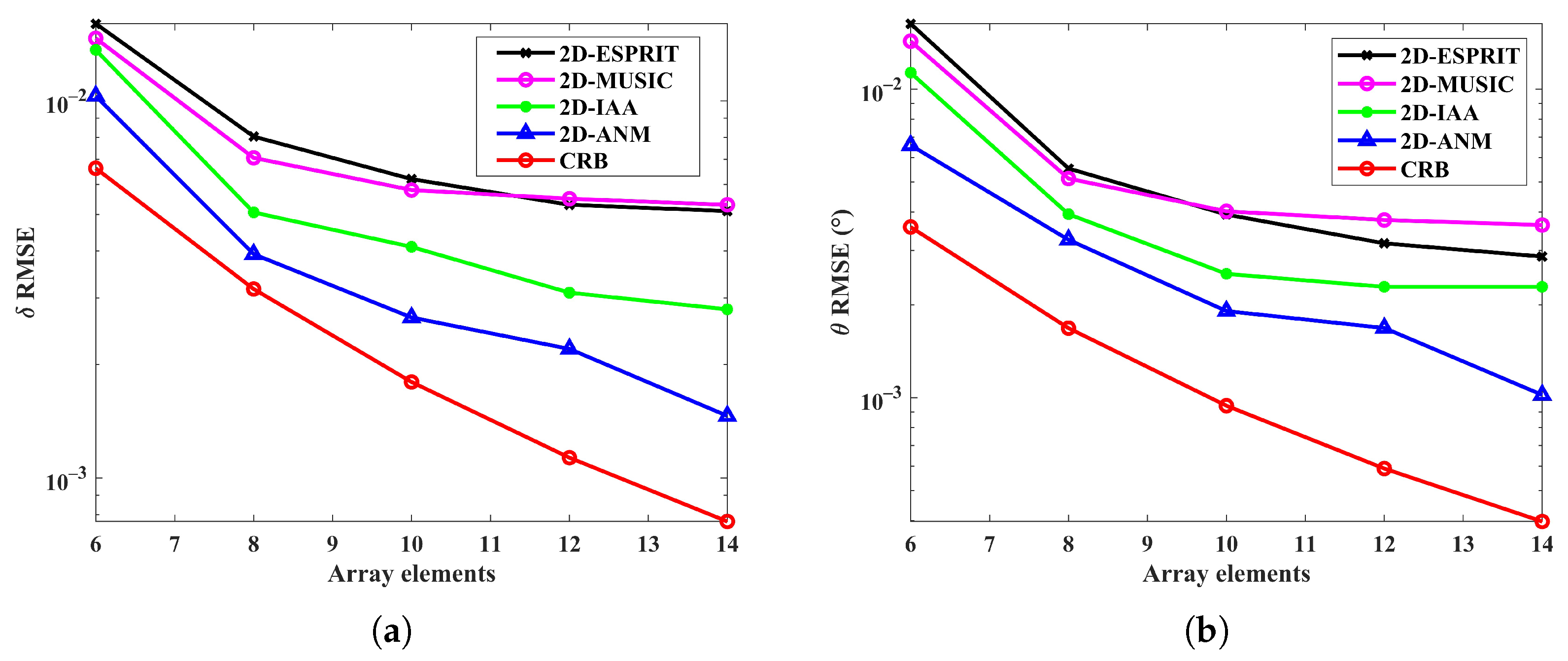
To provide additional insight into the estimation performance of the proposed algorithms, consider setting SNR = 10 dB and varying both the number of array elements and the number of pulses independently, with the results shown in Figure 5 and Figure 6 below. Figure 5 illustrates the RMSE versus the number of array elements for incremental range–angle estimation. As the number of array elements increases, it is evident that the estimation accuracy of both methods enhances, achieving satisfactory performance at high numbers of array elements. However, once the number of array elements reaches a sufficiently high threshold, their performance starts to diverge from the CRB benchmark. Notably, the ANM maintains superior estimation performance. Specifically, with 10 array elements, the ANM achieves performance improvements of at least 1.2 dB, 3.2 dB, and 3.1 dB compared to the 2D-IAA, 2D-MUSIC, and 2D-ESPRIT algorithms, respectively.
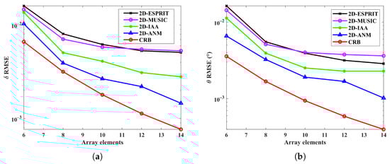
Figure 5.
RMSE versus array elements for parameter estimation: (a) Increment range; (b) Angle.
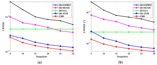
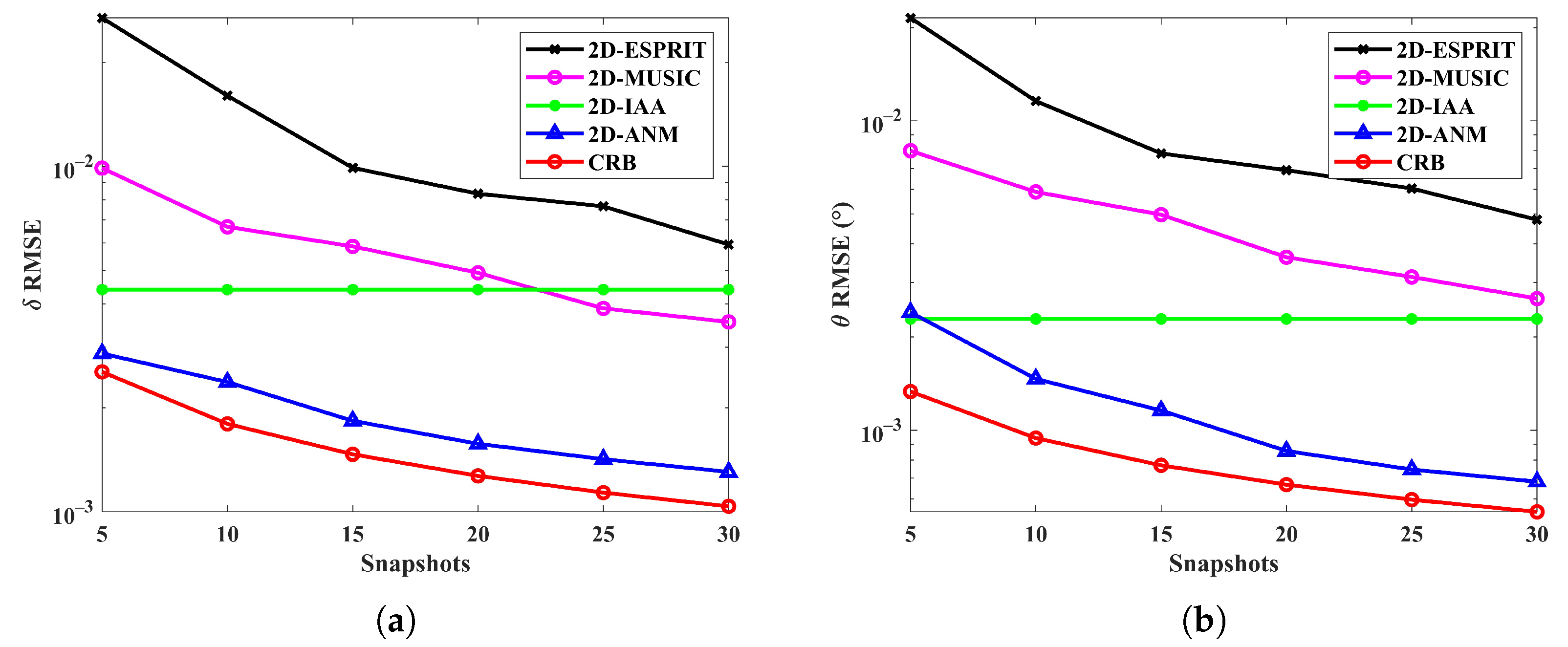
Figure 6.
RMSE versus pulses for parameter estimation: (a) Increment range; (b) Angle.
Figure 6 presents the RMSE curves for angle and increment range estimation of the two algorithms, plotted versus K. Figure 6 illustrates that at low pulse counts, the sparse reconstruction algorithms exhibit notably superior performance compared to the subspace algorithms [58,59]. As K increases, the curve of the ANM algorithm consistently declines, maintaining a trend that aligns closely with the CRB. However, the IAA algorithm shows almost no improvement in estimation performance, and the performance gaps compared to subspace-based algorithms continue to decrease. Notably, when K = 20, the ANM algorithm achieves performance improvements of at least 4.5 dB, 5.0 dB, and 7.2 dB compared to the 2D-IAA, 2D-MUSIC, and 2D-ESPRIT algorithms, respectively.
4.2. Performance Analysis of Target Localization Using Sparse Reconstruction with Distributed Waveform Diverse Array Radars
In this subsection, the localization performance of the distributed waveform diverse array radar system is evaluated. Specifically, the grid partitioning employed by the IAA algorithm aligns with the configurations established in Table 1. The Cartesian coordinates of the targets and radar stations are outlined in Table 2.
Table 2.
Location information in Cartesian coordinates.
Specifically, the distributed waveform diverse array radar system employing the IAA algorithm on its FDA-MIMO radar is termed as distributed radar system 1, whereas the system using the ANM algorithm is termed as distributed radar system 2. Both EPC-MIMO radars in the two distributed systems employ the CD-MUSIC algorithm to obtain the target’s angle and range ambiguity index. Subsequently, the SNR values for the respective stations are configured as −5, 5, and 0, with 200 Monte Carlo trials.
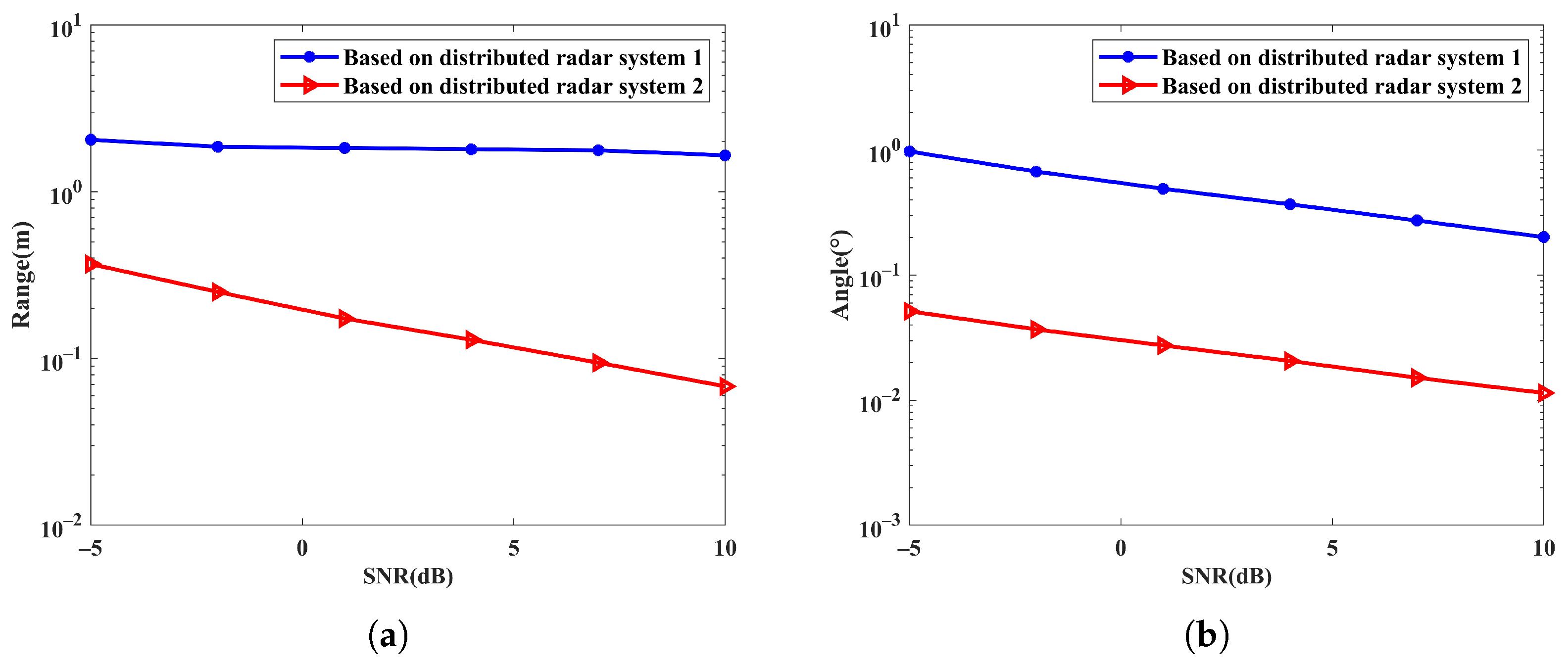
Figure 7 illustrates the RMSEs versus SNR for angle and range estimation of three targets with a distributed waveform diverse array radar system. The RMSEs for range estimation in Figure 7a demonstrate that the two distributed waveform diverse array radar systems achieve excellent estimation performance. Specifically, the ANM-based system achieves a 7.4 dB improvement in estimation performance compared to the IAA-based system at SNR = −5 dB. The RMSE curves for angle estimation in Figure 7b show a continuous decrease as the SNR increases. Notably, the ANM-based system achieves at least a 12.4 dB performance improvement compared to the IAA-based system. In summary, both algorithms demonstrate excellent performance, but the ANM algorithm outperforms the IAA algorithm.
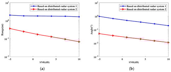
Figure 7.
RMSE versus SNR via distributed waveform–diverse array radars: (a) Range; (b) Angle.
In Figure 8, the estimation results for the angle and range ambiguity index of three targets by distributed waveform diverse array radar systems have been provided. From Figure 8a, it is evident that the curves of the three targets exhibit relatively high peaks, allowing them to be clearly distinguished in the angle dimension. Furthermore, benefiting from the coding of EPC, the range ambiguity is effectively estimated in the distributed radar system, as shown in Figure 8b. It is evident from the numerical results that the RMSE curve is very close to the CRB, which shows that the system has an excellent capability for resolving range ambiguity. As a result, high-precision parameter estimation and resolution of range ambiguity can be achieved simultaneously, demonstrating the superiority of the distributed waveform diverse array radar system for target localization.
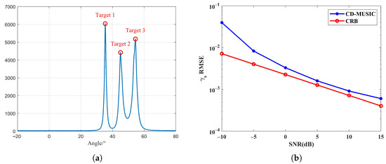
Figure 8.
Estimation via distributed waveform–diverse array radars: (a) Angle; (b) Range ambiguity index.
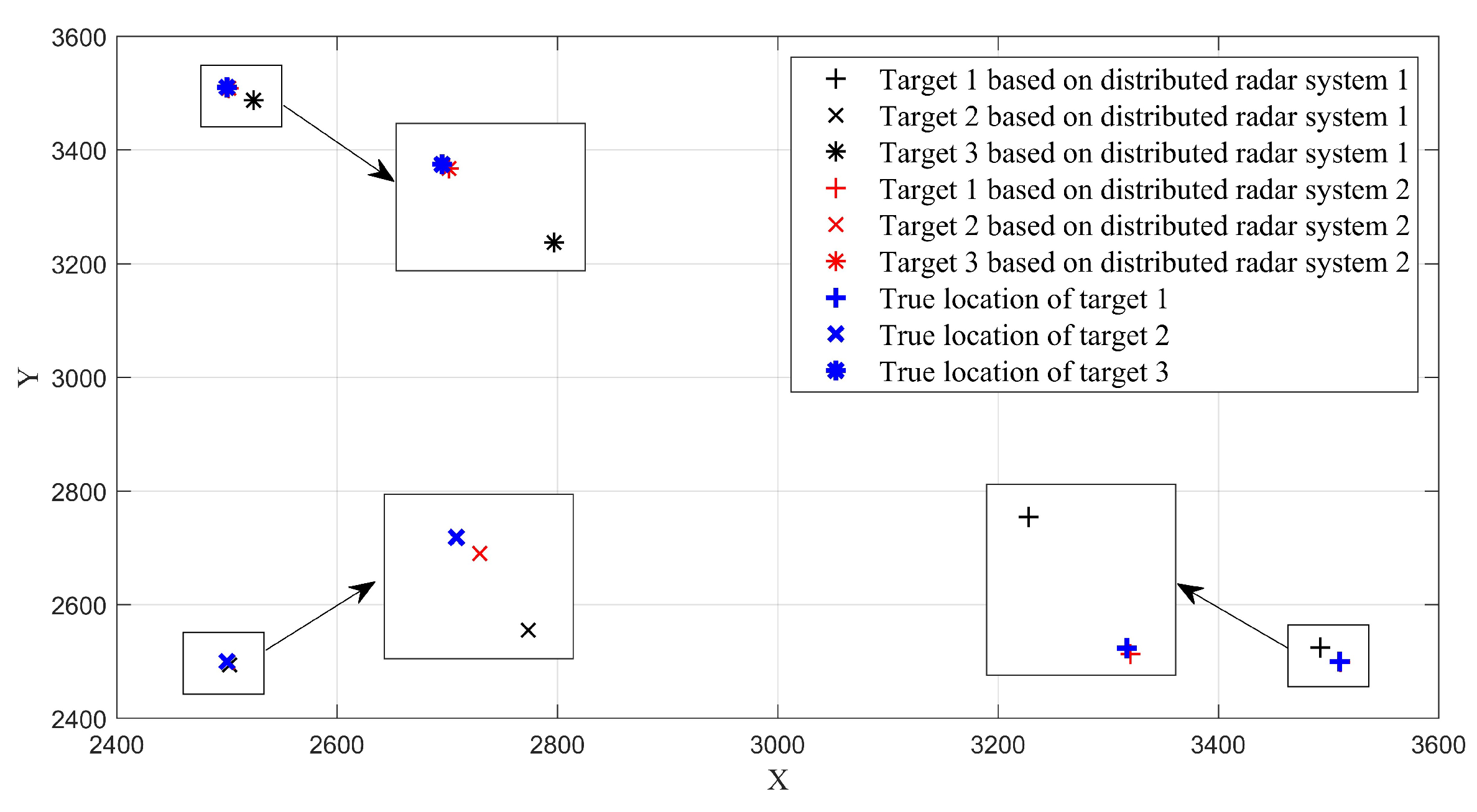
The localization results for three different targets, achieved by two distributed radar systems, are presented in Figure 9. These results represent the average values derived from 200 Monte Carlo experiments. It can be seen that the localization results of the two distributed radar systems are highly accurate, approaching the true target values and demonstrating the capability to localize multiple targets. Upon closer inspection of the enlarged block diagram, it becomes evident that the actual target locations are nearly perfectly aligned with the localization results of distributed radar system 2. As a comparison, the results of system 1 deviate slightly from the true values. Furthermore, considering the aforementioned experimental conditions, it is apparent that distributed radar system 2 exhibits superior localization performance at lower SNR levels. The advantage of the ANM algorithm, particularly in low-SNR environments, is underscored by this observation.
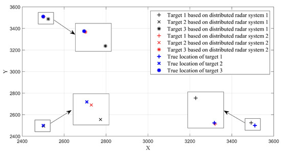
Figure 9.
Target average localization results.
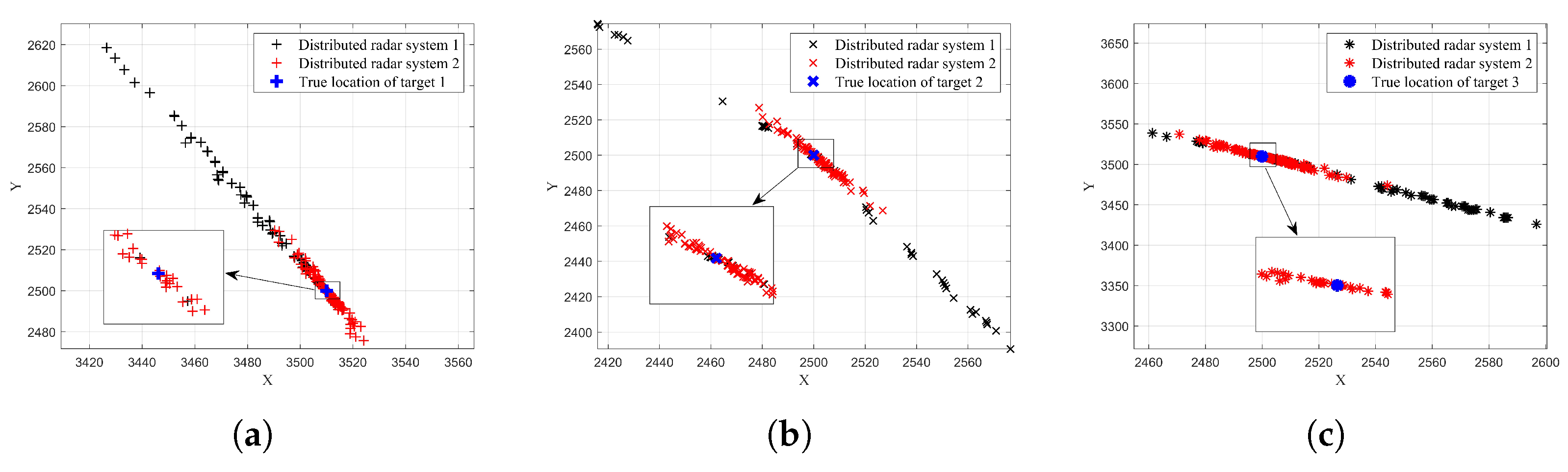
The distribution of localization results for three distinct targets is displayed in Figure 10. It is clear that the dot distributions for all three targets share similar characteristics. In particular, the red dots are close to the true values of each target. In contrast, the black dots are more widely dispersed around the true values, indicating a relatively significant deviation. Thus, in cases of a low SNR and limited snapshots, the superior localization accuracy and robustness of the distributed radar system based on the ANM algorithm are verified.
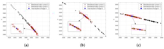
Figure 10.
Distribution map of localization results: (a) Target 1; (b) Target 2; (c) Target 3.
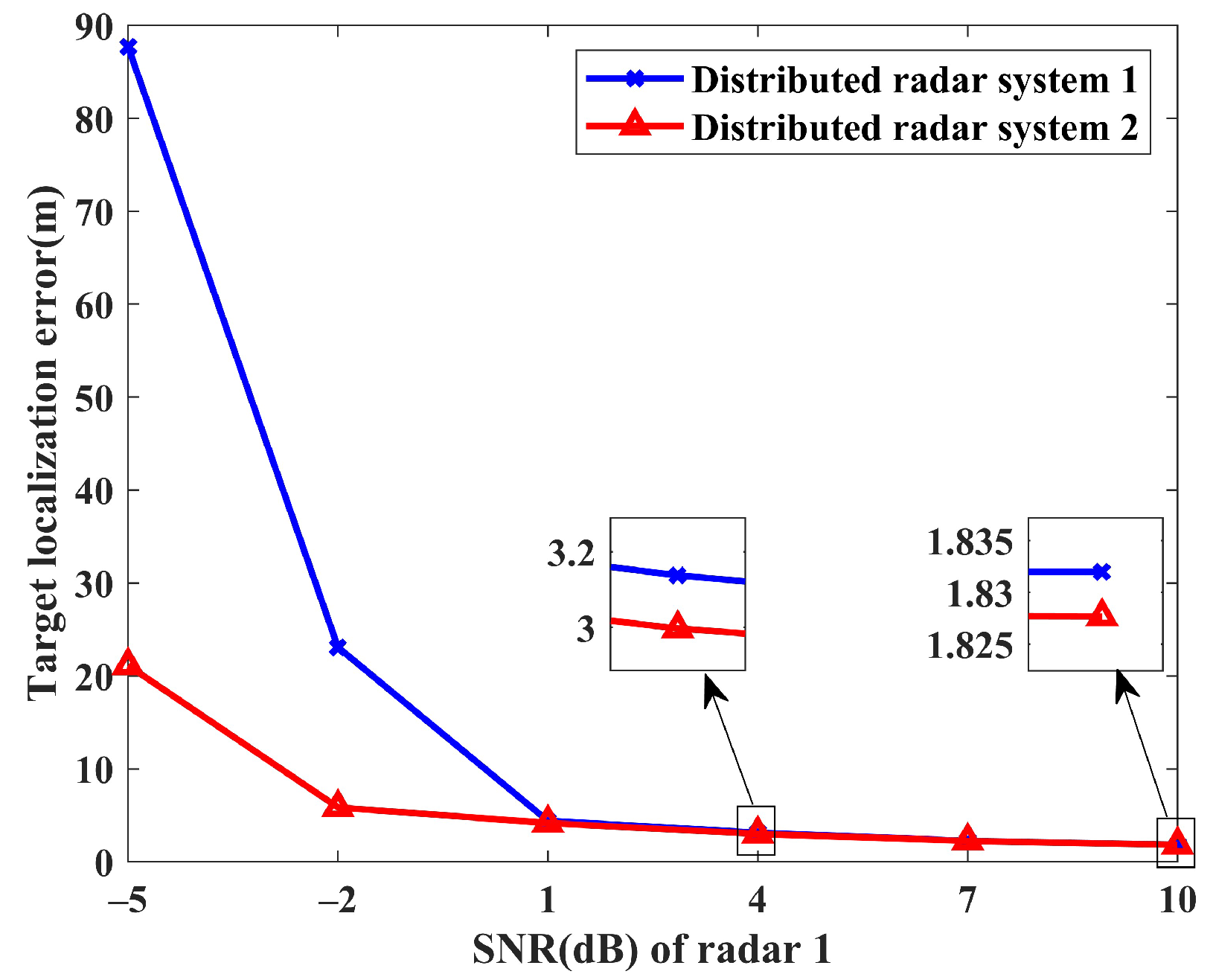
To further validate the localization performance of the methods, the localization results obtained under various SNR scenarios are presented. The baseline dataset, featuring SNR values of [−5, 5, 0], serves as our starting point. Subsequently, the SNR of radar station 1 undergoes adjustment and is systematically elevated. Furthermore, to maintain the SNR ratios observed in the initial dataset, the SNRs of the other two radar stations are also adjusted accordingly. Similarly, 200 Monte Carlo simulations are conducted to verify the estimation accuracy. The average error trends of the three targets versus the SNR variation at radar 1 are shown in Figure 11. Under the same conditions, distributed radar system 2 demonstrates excellent performance improvement compared to system 1. The performance gap between the two systems gradually decreases with an increasing SNR and stabilizes at higher SNRs. Specifically, system 2 achieves a 75.9% improvement in target localization accuracy compared to system 1 at SNR = −5 dB, maintaining this advantage across all evaluated SNR values.
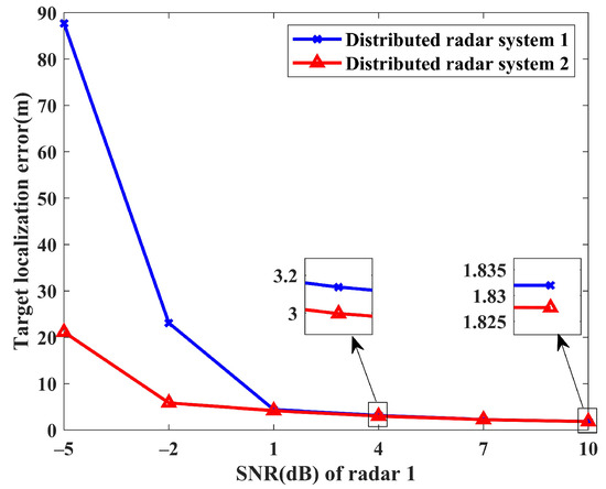
Figure 11.
Target localization error versus SNR.
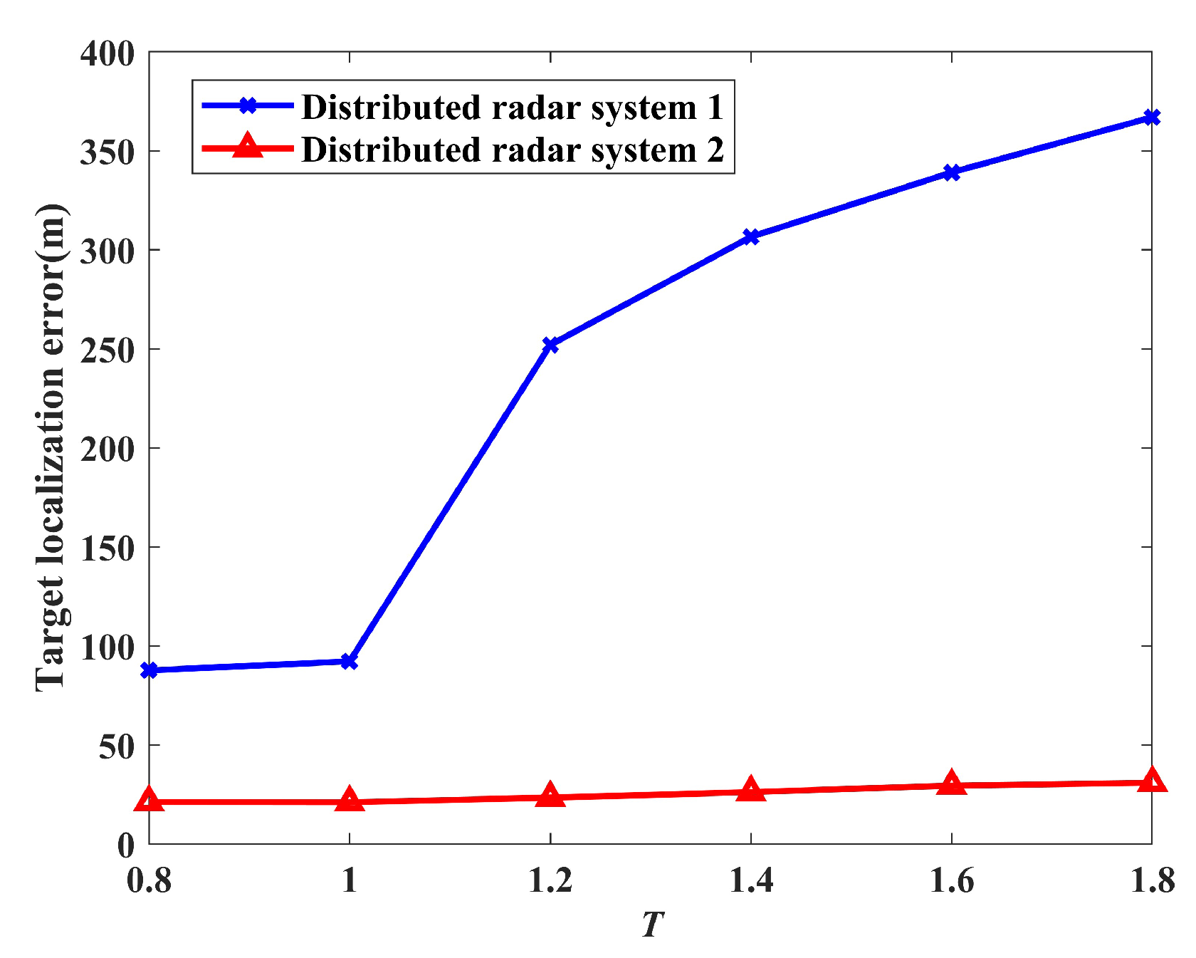
An experimental study was conducted to evaluate the impact of temperature coefficients associated with the weights. The SNRs are set to [−5, 0, 5] dB, with 200 Monte Carlo trials performed. As shown in Figure 12, system 2 exhibits lower localization errors than system 1 under all temperature coefficient conditions, confirming its performance superiority. Specifically, at T = 0.8, the performance gap reaches its minimum, where system 2 achieves a 76% improvement over system 1. As T increases, the performance difference grows rapidly. In summary, the ANM-based system further demonstrates superior target localization accuracy and robust performance across all test conditions.
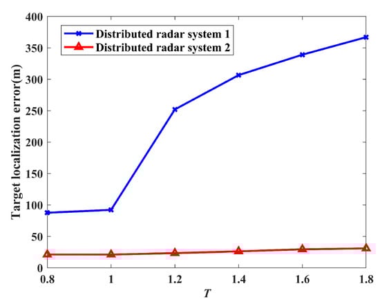
Figure 12.
Target localization error versus temperature coefficient.
5. Conclusions
Target localization based on sparse reconstruction in distributed waveform-diverse array radars, particularly considering low-SNR scenarios, has been investigated. At the design stage, two sparse reconstruction methods are employed at FDA-MIMO radar stations to estimate parameters. Moreover, the WLS method is used by the fusion center to locate the target based on the single-station estimation results. At the analysis stage, the performance of the proposed methods has been assessed based on localization errors, CRBs, and RMSEs. Simulation results show that both single-station and distributed radar systems that employ sparse reconstruction algorithms can accurately localize targets. Significantly, the distributed radar system based on the ANM algorithm demonstrates outstanding localization performance, characterized by excellent accuracy and robustness. The results have shown the effectiveness of the provided methods for target localization in all the considered case studies.
Future research may encompass the introduction of various error conditions, such as spatial registration errors, within the framework of the distributed waveform-diverse array radar architecture. Furthermore, the impact of array errors and mutual coupling in distributed radar systems remains a noteworthy research concern.
Author Contributions
Conceptualization, R.M. and L.L.; methodology, L.L. and G.L.; software, R.M. and F.W.; validation, R.M. and J.X.; formal analysis, J.X. and X.L.; investigation, R.M. and X.L.; resources, L.L. and G.L.; data curation, L.L. and G.L.; writing—original draft preparation, R.M.; writing—review and editing, R.M. and L.L.; visualization, R.M. and F.W.; supervision, L.L. and G.L.; project administration, L.L. and G.L.; funding acquisition, L.L. and G.L. All authors have read and agreed to the published version of the manuscript.
Funding
This work was supported in part by the National Nature Science Foundation of China (Nos. 62471348 and 62431021), the Fundamental Research Funds for the Central Universities (No. QTZX23068), and the Young Science and Technology Star of Shaanxi Province (No. 2024ZC-KJXX-009).
Data Availability Statement
The original contributions presented in this study are included in the article.
Conflicts of Interest
The authors declare no conflicts of interest.
Appendix A
Appendix A.1. Details on CRB for the FDA-MIMO Radar
According to Equation (22), the first derivatives of w.r.t. and can be calculated as
and
where , , and with and .
Let us consider
The entries of are given as follows
and
Therefore, is given as
with
and
Appendix A.2. Details on CRB for the EPC-MIMO Radar
Let us consider , where the entries of are given as follows
and
Therefore, is given as
with
and
References
- Peng, Y.; Ding, Y.; Cao, J.; Tang, B.; Jiang, Y. Doppler Radar-Based Target Localization Algorithm Combining Adaptive Linear Chirplet Transform and Frequency Compensation. IEEE Trans. Aerosp. Electron. Syst. 2025, 61, 2057–2067. [Google Scholar] [CrossRef]
- Grossi, E.; Taremizadeh, H.; Venturino, L. Radar Target Detection and Localization Aided by an Active Reconfigurable Intelligent Surface. IEEE Signal Process. Lett. 2023, 30, 903–907. [Google Scholar] [CrossRef]
- Chen, R.; Guo, S.; Chen, J.; Gu, X.; Cui, G.; Kong, L.; Liu, W. Low-Complexity Multitarget Detection and Localization Method for Distributed MIMO Radar. IEEE Trans. Radar Syst. 2025, 3, 599–614. [Google Scholar] [CrossRef]
- Rosamilia, M.; Balleri, A.; Maio, A.D.; Aubry, A.; Carotenuto, V. Radar Detection Performance Prediction Using Measured UAVs RCS Data. IEEE Trans. Aerosp. Electron. Syst. 2023, 59, 3550–3565. [Google Scholar] [CrossRef]
- Mao, Z.; Su, H.; Song, J.; Han, K. Joint Target and Transmitter Localization with AOA and DTD Using Passive Sensors. IEEE Signal Process. Lett. 2024, 31, 1570–1574. [Google Scholar] [CrossRef]
- Wang, H.; Chen, Z.; Zheng, S. Preliminary Research of Low-RCS Moving Target Detection Based on Ka-Band Video SAR. IEEE Geosci. Remote Sens. Lett. 2017, 14, 811–815. [Google Scholar] [CrossRef]
- Cao, X.; Yi, J.; Gong, Z.; Wan, X. Automatic Target Recognition Based on RCS and Angular Diversity for Multistatic Passive Radar. IEEE Trans. Aerosp. Electron. Syst. 2022, 58, 4226–4240. [Google Scholar] [CrossRef]
- Mertens, M.; Ulmke, M.; Koch, W. Ground target tracking with RCS estimation based on signal strength measurements. IEEE Trans. Aerosp. Electron. Syst. 2016, 52, 205–220. [Google Scholar] [CrossRef]
- Shi, C.; Wang, Y.; Salous, S.; Zhou, J.; Yan, J. Joint Transmit Resource Management and Waveform Selection Strategy for Target Tracking in Distributed Phased Array Radar Network. IEEE Trans. Aerosp. Electron. Syst. 2022, 58, 2762–2778. [Google Scholar] [CrossRef]
- Zhang, Z.; Zhou, J.; Wang, F.; Liu, W.; Yang, H. Multiple-target tracking with adaptive sampling intervals for phased-array radar. J. Syst. Eng. Electron. 2011, 22, 760–766. [Google Scholar] [CrossRef]
- Shi, C.; Ding, L.; Wang, F.; Salous, S.; Zhou, J. Joint Target Assignment and Resource Optimization Framework for Multitarget Tracking in Phased Array Radar Network. IEEE Syst. J. 2021, 15, 4379–4390. [Google Scholar] [CrossRef]
- Lan, L.; Xu, J.; Liao, G.; Zhang, Y.; Fioranelli, F.; So, H.C. Suppression of Mainbeam Deceptive Jammer with FDA-MIMO Radar. IEEE Trans. Veh. Technol. 2020, 69, 11584–11598. [Google Scholar] [CrossRef]
- Lan, L.; Xu, J.; Liao, G.; Zhu, S.; So, H.C. Mainlobe Deceptive Jammer Suppression in SF-RDA Radar: Joint Transmit-Receive Processing. IEEE Trans. Veh. Technol. 2022, 71, 12602–12616. [Google Scholar] [CrossRef]
- Zhu, J.; Zhu, S.; Xu, J.; Lan, L. Discrimination of Target and Mainlobe Jammers with FDA-MIMO Radar. IEEE Signal Process. Lett. 2023, 30, 583–587. [Google Scholar] [CrossRef]
- Jing, X.; Su, H.; Li, Z.; Yang, R.; Zhu, Y. Weak Moving Target Detection in Distributed MIMO Radar with Hybrid Data. IEEE Trans. Aerosp. Electron. Syst. 2024, 60, 9291–9306. [Google Scholar] [CrossRef]
- Li, Z.; Ding, Z.; Wang, Y.; Sun, Y.; Li, L. Space Target Detection Based on DBF and GRFT for Ground-Based Distributed Radar. IEEE Geosci. Remote Sens. Lett. 2024, 21, 3504105. [Google Scholar] [CrossRef]
- Yu, Z.; Li, J.; Guo, Q.; Ding, J. Efficient Direct Target Localization for Distributed MIMO Radar with Expectation Propagation and Belief Propagation. IEEE Trans. Signal Process. 2021, 69, 4055–4068. [Google Scholar] [CrossRef]
- Tirer, T.; Weiss, A.J. High Resolution Direct Position Determination of Radio Frequency Sources. IEEE Signal Process. Lett. 2016, 23, 192–196. [Google Scholar] [CrossRef]
- Sadeghi, M.; Behnia, F.; Amiri, R.; Farina, A. Target Localization Geometry Gain in Distributed MIMO Radar. IEEE Trans. Signal Process. 2021, 69, 1642–1652. [Google Scholar] [CrossRef]
- Xie, R.; Luo, K.; Jiang, T. Joint Coverage and Localization Driven Receiver Placement in Distributed Passive Radar. IEEE Trans. Geosci. Remote Sens. 2021, 59, 1094–1105. [Google Scholar] [CrossRef]
- Zhou, Q.; Yuan, Y.; Venturino, L.; Yi, W. Direct Target Localization for Distributed Passive Radars with Direct-Path Interference Suppression. IEEE Trans. Signal Process. 2024, 72, 3611–3625. [Google Scholar] [CrossRef]
- Xia, N.; Xiang, R.; Xing, B.; Gao, D. TDOA Based Direct Positioning of Co-Channel Signals Using Cyclic Cross-Spectral Functions. IEEE Commun. Lett. 2024, 28, 303–307. [Google Scholar] [CrossRef]
- Keskin, M.F.; Gezici, S.; Arikan, O. Direct and Two-Step Positioning in Visible Light Systems. IEEE Trans. Commun. 2018, 66, 239–254. [Google Scholar] [CrossRef]
- Zhu, K.; Jiang, H.; Li, J.; Zhou, F. A Direct Position Determination Method Using Distributed UAVs with Synchronization Error. IEEE Sens. J. 2024, 24, 780–787. [Google Scholar] [CrossRef]
- Song, H.; Wen, G.; Zhu, L.; Li, D. A Novel TSWLS Method for Moving Target Localization in Distributed MIMO Radar Systems. IEEE Commun. Lett. 2019, 23, 2210–2214. [Google Scholar] [CrossRef]
- Zhu, L.; Wen, G.; Liang, Y.; Luo, D.; Jian, H. Multitarget Enumeration and Localization in Distributed MIMO Radar Based on Energy Modeling and Compressive Sensing. IEEE Trans. Aerosp. Electron. Syst. 2023, 59, 4493–4510. [Google Scholar] [CrossRef]
- Lan, L.; Rosamilia, M.; Aubry, A.; De Maio, A.; Liao, G. FDA-MIMO Transmitter and Receiver Optimization. IEEE Trans. Signal Process. 2024, 72, 1576–1589. [Google Scholar] [CrossRef]
- Zhu, J.; Zhu, S.; Xu, J.; Lan, L.; He, X. Cooperative Range and Angle Estimation with PA and FDA Radars. IEEE Trans. Aerosp. Electron. Syst. 2022, 58, 907–921. [Google Scholar] [CrossRef]
- Lan, L.; Rosamilia, M.; Aubry, A.; De Maio, A.; Liao, G. FDA-MIMO Transceiver Design Under the Uniform Frequency Increment Constraint. IEEE Trans. Radar Syst. 2024, 2, 446–459. [Google Scholar] [CrossRef]
- Gui, R.; Wang, W.-Q.; Pan, Y.; Xu, J. Cognitive Target Tracking via angle-range-Doppler Estimation with Transmit Subaperturing FDA Radar. IEEE J. Sel. Top. Signal Process. 2018, 12, 76–89. [Google Scholar] [CrossRef]
- Yu, K.; Zhu, S.; Lan, L.; Xu, J.; Li, X. Resolving Range Ambiguity Using Transmit Coding Modulation and Multi-Pulse Processing in FPC-PA Radar. IEEE Trans. Veh. Technol. 2024, 73, 11168–11181. [Google Scholar] [CrossRef]
- Lan, L.; Rosamilia, M.; Aubry, A.; Maio, A.D.; Liao, G. Single-Snapshot Angle and Incremental Range Estimation for FDA-MIMO Radar. IEEE Trans. Aerosp. Electron. Syst. 2021, 57, 3705–3718. [Google Scholar] [CrossRef]
- Lan, L.; Zhang, Y.; Liao, R.; Liao, G.; Xu, J.; So, H.C. Mainlobe Deceptive Jammer Mitigation with Multipath in EPC-MIMO Radar Exploiting Matrix Decomposition. IEEE Trans. Veh. Technol. 2024, 73, 14674–14688. [Google Scholar] [CrossRef]
- Xu, J.; Zhang, Y.; Liao, G.; So, H.C. Resolving Range Ambiguity via Multiple-Input Multiple-Output Radar with Element-Pulse Coding. IEEE Trans. Signal Process. 2020, 68, 2770–2783. [Google Scholar] [CrossRef]
- Gao, J.; Zhu, S.; Lan, L.; Sui, J.; Li, X. Range-Ambiguous Clutter Separation via Reweighted Atomic Norm Minimization with EPC-MIMO Radar. IEEE Trans. Signal Process. 2025, 32, 146–150. [Google Scholar] [CrossRef]
- Xing, W.; Zhou, C.; Wang, C. Modified OMP method for multi-target parameter estimation in frequency-agile distributed MIMO radar. J. Syst. Eng. Electron. 2022, 33, 1089–1094. [Google Scholar] [CrossRef]
- Chen, H.; Shao, H. Sparse reconstruction based target localization with frequency diverse array MIMO radar. In Proceedings of the 2015 IEEE China Summit and International Conference on Signal and Information Processing (ChinaSIP), Chengdu, China, 12–15 July 2015; pp. 94–98. [Google Scholar]
- Xiong, J.; Wang, W.-Q. Sparse reconstruction-based beampattern synthesis for multi-carrier frequency diverse array antenna. In Proceedings of the 2017 IEEE International Conference on Acoustics, Speech and Signal Processing (ICASSP), New Orleans, LA, USA, 5–9 March 2017; pp. 3395–3398. [Google Scholar]
- Tang, W.-G.; Jiang, H.; Zhang, Q. Range-Angle Decoupling and Estimation for FDA-MIMO Radar via Atomic Norm Minimization and Accelerated Proximal Gradient. IEEE Signal Process. Lett. 2020, 27, 366–370. [Google Scholar] [CrossRef]
- Tang, W.-G.; Jiang, H.; Pang, S.-X. Grid-Free DOD and DOA Estimation for MIMO Radar via Duality-Based 2D Atomic Norm Minimization. IEEE Access 2019, 7, 60827–60836. [Google Scholar] [CrossRef]
- Malanowski, M.; Kulpa, K. Two Methods for Target Localization in Multistatic Passive Radar. IEEE Trans. Aerosp. Electron. Syst. 2012, 48, 572–580. [Google Scholar] [CrossRef]
- Zhang, Y.; Zhang, Y.; Huang, Y.; Li, W.; Yang, J. Angular Superresolution for Scanning Radar with Improved Regularized Iterative Adaptive Approach. IEEE Geosci. Remote Sens. Lett. 2016, 13, 846–850. [Google Scholar] [CrossRef]
- Luo, J.; Huang, Y.; Zhang, Y.; Tuo, X.; Zhang, D. Two-Dimensional Angular Super-Resolution for Airborne Real Aperture Radar by Fast Conjugate Gradient Iterative Adaptive Approach. IEEE Access 2023, 59, 9480–9500. [Google Scholar] [CrossRef]
- Tian, J.; Zhang, B.; Cui, W.; Wu, S. Joint Iterative Adaptive Approach for Sidelobe Suppression and Migration Correction of Migrating Targets. IEEE Trans. Aerosp. Electron. Syst. 2025, 61, 2973–2995. [Google Scholar] [CrossRef]
- Zhang, X.; Zheng, Z.; Wang, W.-Q.; So, H.C. DOA Estimation of Coherent Sources Using Coprime Array via Atomic Norm Minimization. IEEE Signal Process. Lett. 2022, 29, 1312–1316. [Google Scholar] [CrossRef]
- Yang, Z.; Xie, L. Enhancing Sparsity and Resolution via Reweighted Atomic Norm Minimization. IEEE Trans. Signal Process. 2016, 64, 995–1006. [Google Scholar] [CrossRef]
- Hu, X.; Tong, N.; Zhang, Y.; He, X.; Wang, Y. Moving Target’s HRRP Synthesis with Sparse Frequency-Stepped Chirp Signal via Atomic Norm Minimization. IEEE Signal Process. Lett. 2016, 23, 1212–1215. [Google Scholar] [CrossRef]
- Dianat, M.; Taban, M.R.; Dianat, J.; Sedighi, V. Target Localization Using Least Squares Estimation for MIMO Radars with Widely Separated Antennas. IEEE Trans. Aerosp. Electron. Syst. 2013, 49, 2730–2741. [Google Scholar] [CrossRef]
- Lan, L.; Marino, A.; Aubry, A.; Maio, A.D.; Liao, G.; Xu, J. GLRT-Based Adaptive Target Detection in FDA-MIMO Radar. IEEE Trans. Aerosp. Electron. Syst. 2021, 57, 597–613. [Google Scholar] [CrossRef]
- Glentis, G.-O.; Jakobsson, A. Efficient Implementation of Iterative Adaptive Approach Spectral Estimation Techniques. IEEE Trans. Signal Process. 2011, 59, 4154–4167. [Google Scholar] [CrossRef]
- Zhang, Y.; Jakobsson, A.; Yang, J. Range-Recursive IAA for Scanning Radar Angular Super-Resolution. IEEE Geosci. Remote Sens. Lett. 2017, 14, 1675–1679. [Google Scholar] [CrossRef]
- Tian, J.; Zhang, B.; Li, K.; Cui, W.; Wu, S. Low-Complexity Iterative Adaptive Approach Based on Range–Doppler Matched Filter Outputs. IEEE Trans. Aerosp. Electron. Syst. 2023, 59, 125–139. [Google Scholar] [CrossRef]
- Chi, Y.; Chen, Y. Compressive Two-Dimensional Harmonic Retrieval via Atomic Norm Minimization. IEEE Trans. Signal Process. 2015, 63, 1030–1042. [Google Scholar] [CrossRef]
- Donoho, D.L. Compressed sensing. IEEE Trans. Inf. Theory 2006, 52, 1289–1306. [Google Scholar] [CrossRef]
- Yang, Y.; Chu, Z.; Ping, G. Two-dimensional multiple-snapshot grid-free compressive beamforming. Mech. Syst. Sig. Process. 2019, 124, 524–540. [Google Scholar] [CrossRef]
- Yang, Z.; Xie, L. Exact joint sparse frequency recovery via optimizabtion methods. IEEE Trans. Signal Process. 2016, 64, 5145–5157. [Google Scholar] [CrossRef]
- Yang, Z.; Xie, L.; Stoica, P. Vandermonde decomposition of multilevel Toeplitz matrices with application to multidimensional super-resolution. IEEE Trans. Inf. Theory 2016, 62, 3685–3701. [Google Scholar] [CrossRef]
- Liu, Z.; Wu, J.; Yang, S.; Lu, W. DOA Estimation Method Based on EMD and MUSIC for Mutual Interference in FMCW Automotive Radars. IEEE Geosci. Remote Sens. Lett. 2022, 19, 3504005. [Google Scholar] [CrossRef]
- Hu, Y.; Deng, W.; Zhang, X.; Wu, X. FDA-MIMO Radar with Long-Baseline Transmit Array Using ESPRIT. IEEE Signal Process. Lett. 2021, 28, 1530–1534. [Google Scholar] [CrossRef]
- De Maio, A.; Orlando, D. Adaptive Radar Detection of a Subspace Signal Embedded in Subspace Structured Plus Gaussian Interference via Invariance. IEEE Trans. Signal Process. 2016, 64, 2156–2167. [Google Scholar] [CrossRef]


Disclaimer/Publisher’s Note: The statements, opinions and data contained in all publications are solely those of the individual author(s) and contributor(s) and not of MDPI and/or the editor(s). MDPI and/or the editor(s) disclaim responsibility for any injury to people or property resulting from any ideas, methods, instructions or products referred to in the content. |
© 2025 by the authors. Licensee MDPI, Basel, Switzerland. This article is an open access article distributed under the terms and conditions of the Creative Commons Attribution (CC BY) license (https://creativecommons.org/licenses/by/4.0/).