Highlights
What are the main findings?
- Bathymetric maps generated by 1D-CNN models and hyperspectral images consistently reproduced the expected depth gradient from nearshore to offshore and seabed morphologies with high resolution.
- Band optimization implementation reduced computational requirements by 31–38%.
What is the implication of the main finding?
- The Band optimization Pansharpening CNN (BoPsCNN) model is a promising tool for deriving high-resolution shallow bathymetry from hyperspectral remote sensing data.
- The proposed innovative methodology is suitable for moderately turbid waters.
Abstract
The combined application of machine or deep learning algorithms and hyperspectral imagery for bathymetry estimation is currently an emerging field with widespread uses and applications. This research topic still requires further investigation to achieve methodological robustness and accuracy. In this study, we introduce a novel methodology for shallow bathymetric mapping using a one-dimensional convolutional neural network (1D-CNN) applied to PRISMA hyperspectral images, including refinements to enhance mapping accuracy, together with the optimization of computational efficiency. Four different 1D-CNN models were developed, incorporating pansharpening and spectral band optimization. Model performance was rigorously evaluated against reference bathymetric data obtained from official nautical charts provided by the Servicio de Hidrografía Naval (Argentina). The BoPsCNN model achieved the best testing accuracy with a coefficient of determination of 0.96 and a root mean square error of 0.65 m for a depth range of 0–15 m. The implementation of band optimization significantly reduced computational overhead, yielding a time-saving efficiency of 31–38%. The resulting bathymetric maps exhibited a coherent depth gradient from nearshore to offshore zones, with enhanced seabed morphology representation, particularly in models using pansharpened data.
1. Introduction
Accurate bathymetric mapping is critical for diverse applications, including oceanographic and coastal zone research, maritime navigation, port and harbor management, and the planning and maintenance of submarine pipelines and telecommunication cables, among many others [1]. Traditional bathymetric surveys rely on acoustic and Light Detection and Ranging (LiDAR). In the last decade, emerging trends in seafloor depth measurement focused on integrating multiple instruments, platforms, and techniques. Notable approaches include bathymetric LiDAR systems deployed on aerial vehicles [2,3,4], bathymetric structure-from-motion (SfM) photogrammetry using Remotely Operated Vehicles (ROVs) [5], bathymetric SfM photogrammetry using Unmanned Surface Vehicles (USVs) [6,7], and bathymetric echo-sounding systems mounted on USVs [8,9,10]. Each combination presents distinct advantages and limitations in terms of resolution, coverage, accuracy, operational complexity, and upfront and operational costs. However, surveying expenses—including equipment procurement and operational expenditures—remain prohibitively high, particularly in research groups from developing countries.
Additionally, significant efforts were directed towards deriving bathymetric data from remote sensing imagery, mainly due to its capacity for extensive spatial coverage and lower acquisition costs. These techniques leverage both active synthetic aperture radar (SAR) and passive optical modalities. SAR measures RADAR backscatter from the ocean surface, enabling depth estimation down to 100–200 m [11], although there is evidence of the SAR imaging of bathymetry at depths > 500 m in the Gulf Stream [12]. Advancements in passive optical remote sensing—utilizing Earth-orbiting satellites or aircraft systems— spurred considerable interest in high-resolution bathymetric mapping [13]. These passive techniques rely on measuring natural light reflected from the seafloor and retrodispersed through the optical path. The propagation of optical and infrared radiation in water is governed by complex interactions involving atmospheric conditions, water turbidity, depth attenuation, and seafloor reflectance [14]. Consequently, only a minimal fraction of incident solar radiation is backscattered and detectable by remote sensors. In most coastal regions, water clarity is reduced by colored substances (e.g., sediment, algae, etc.) where depths up to a few meters can be measured [15]. This methodology operates on the principle that surface water color can indicate turbidity, which is related to a given depth [11].
Image analysis and processing plays a crucial role in the accurate estimation of bathymetric data. Recent advances in statistical modeling and machine learning or deep learning techniques demonstrated high accuracy in processing multispectral or hyperspectral image data. A key result was to establish nonlinear relationships between spectral signatures and water depths, facilitating the generation of bathymetric maps mainly in coastal regions [16,17]. In this context, preprocessing steps before model training are primarily designed to enhance data quality and optimize computational efficiency. Among these preprocessing steps, pansharpening is one of the most used methods for improving quality and consists of fusing the spatial detail of a high resolution panchromatic image and the spectral information of a low resolution multi/hyperspectral image to create a fused image product [18]. As outlined in the comprehensive review by Loncan et al. [19] about pansharpening applications, the predominant methods include component substitution, multiresolution analysis, and hybrid approaches. For example, Karimi et al. [20] applied a hybrid pansharpening method to enhance bathymetric mapping in coastal areas.
On the other hand, there are methods that involve hyperspectral band selection to remove spectral redundancy and reduce computational costs [3]. For example, Qi et al. [21] proposed an unsupervised band selection method by embedding the bathymetric model into the band selection process, which showed effectiveness and efficiency in comparison with other methods. Xi et al. [22] focused on the application of dual-band selection and multi-band selection algorithms to select the band ratios and the most important bands, respectively.
Machine and deep learning algorithms were successfully applied to derive bathymetric data in shallow waters using multispectral or hyperspectral imagery. For instance, Sun et al. [16] developed a deep convolutional neural network (CNN)-based bathymetry model for shallow water regions, using Sentinel-2 and WorldView-2 multispectral images with LiDAR and sonar data as reference. Their findings demonstrated that CNN models achieved low prediction errors, particularly when enhanced with nonlinear normalization techniques. Wang et al. [23] focused on the use of PRISMA hyperspectral and Sentinel-2 and Landsat 9 multispectral images for bathymetry inversion using an attention-based band optimization 1D-CNN model, with ICESat-2 and imaging spectroscopy data as reference data. Their results indicated superior retrieval accuracy within the 0–20 m depth range by using PRISMA hyperspectral data. Another contribution is the work of Xie et al. [17], who introduced a physics-informed CNN model trained on Sentinel-2 multispectral imagery and ICESat-2 reference data, incorporating radiative transfer principles. This approach yielded bathymetric maps with mean errors under 1.60 m, demonstrating the efficacy of integrating physical constraints into machine learning frameworks.
Given that the application of machine and deep learning algorithms for bathymetric estimation from multispectral or hyperspectral imagery remains an emergent research area, further methodological refinements are imperative to provide robust and accurate estimates. To address this imperative, the present study introduces an innovative framework for bathymetric estimation in shallow water environments, leveraging 1D-CNN applied to PRISMA hyperspectral data. Four 1D-CNN models were developed and applied in two study areas, incorporating enhancement methods such as pansharpening and band optimization. The models are called CNN, Pansharpening CNN (PsCNN), Band optimization CNN (BoCNN), and Band optimization Pansharpening CNN (BoPsCNN). The performance of these models was subsequently assessed in terms of coefficient of determination (), mean absolute error (MAE), and root mean square error (RMSE) against reference bathymetry from official nautical charts provided by the Servicio de Hidrografía Naval (SHN [24]), Argentina.
2. Materials and Methods
The flowchart in Figure 1 outlines the overall procedure and the applied methods and techniques for the bathymetry estimation. It can be divided into three broad stages: (1) data input preprocessing, (2) bathymetry estimation process, and (3) performance assessment.
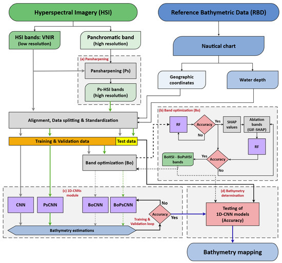
Figure 1.
Flowchart of the overall procedure, methods, and techniques for the bathymetry estimation: (a) Pansharpening module; (b) Band optimization (Bo) module; (c) 1D-CNN module: CNN, Pansharpening CNN (PsCNN), Band optimization CNN (BoCNN), and Band optimization Pansharpening CNN (BoPsCNN); (d) Bathymetry estimation (accuracy on test data), and Bathymetry mapping. Accuracy is evaluated in terms of R2, MAE, and RMSE. RF: Random Forest. SHAP: SHapley Additive exPlanations. GIF-SHAP: Global Importance Factor SHAP. HSI: Hyperspectral imagery. Ps-HSI: Pansharpened HSI. BoHSI: Band-optimized HSI. BoPsHSI: Band optimized Pansharpened HSI. Note: Gray and green arrows indicate hyperspectral datasets without and with pansharpening, respectively; Solid and dotted arrows represent datasets without and with optimized bands, in that order.
2.1. Study Area
For the purpose of this research, two coastal shallow areas (CA#1 and CA#2) located in the Argentine sea were selected (Figure 2). The CA#1 includes the San Borombón open bay at the outer part of the Río de la Plata estuary, in the northeastern Buenos Aires province coast (Figure 2). In the outer estuary, the turbidity observed is low (<10 FNU -Formazin Nephelometric Units-) mainly due to flocculation and deposition of sediments at the tip of the bottom salinity front [25]. A turbidity front strongly related to the bathymetry enters into the San Borombón bay as a narrow plume close to the coastline [25,26]. The tidal regime is semidiurnal and microtidal, with a mean tidal range of approximately 0.76 m [24]. The remaining study area (CA#2) is an open coast in the southwestern Buenos Aires province coast (Bahía Blanca bay); the west of the CA#2 is bordered by the outer part of the Bahía Blanca estuary (Figure 2). According to Arena et al. [27], from a synoptic-scale perspective, the average turbidity shows a sharp transition from the turbid waters characterizing the inner estuary to the clearer water conditions typical of the coastal zone out of the estuary. The tidal regime is semidiurnal and mesotidal, with a mean tidal range of approximately 2.3 m [24].
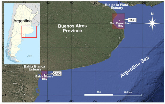
Figure 2.
Localization of the study areas: San Borombón bay (CA#1) and Bahía Blanca bay (CA#2). Base map provided by freely available Google Earth mapping service.
2.2. Image Input and Preprocessing
2.2.1. Satellite Hyperspectral Data
The PRISMA satellite launched by the Italian Space Agency provides 66 bands in the Visible Near Infra-red (VNIR) range and 173 bands in the shortwave infrared (SWIR) range, over a continuum from 400 to 2500 nm, with a spatial resolution of 30 m. In addition, PRISMA provides a panchromatic image (400–700 nm) of 5 m spatial resolution. In this study, VNIR bands, together with the panchromatic band, were utilized. PRISMA L2D cloud-free images were used; L2D level is a geolocated, geocoded, and orthorectified surface reflectance product. Table 1 shows the list of the images used in this study.

Table 1.
PRISMA images used in this study.
2.2.2. Image Quality
The image quality of hyperspectral imagery (HSI) was evaluated in terms of image signal-to-noise ratio (SNR), which is a standard quantitative metric for evaluating radiometric reliability in hyperspectral imagery. The SNR was computed as the logarithmic ratio between the mean signal () and its standard deviation (), using the following equation:
This formulation reflects the radiometric stability of each band, where higher SNR values indicate greater signal uniformity and low noise influence. To ensure that only bands containing meaningful information were included in further analysis, a band band-wise quality screening was performed by applying a range of SNR thresholds above 0 dB. Thresholds below 0 dB typically denote that random noise dominates over the true signal, leading to unreliable reflectance estimates.
Initial analysis revealed that three bands centered at 987, 998, and 1009 nm exhibited SNR values below 0.05 dB. Visual inspection of these bands confirmed the absence of discernible spatial patterns or spectral information, indicating that they were effectively null bands dominated by sensor noise or signal attenuation near the upper limit of the spectral range. To verify the robustness of this threshold, the SNR criterion was incrementally increased. The next lowest band above 0 dB, centered at 474 nm (0.08 dB), displayed spatially coherent information consistent with expected scene features, and was therefore retained. Consequently, an SNR threshold of 0.05 dB was adopted as a conservative yet objective criterion for filtering out null or excessively noisy bands. This threshold balances the need to remove non-informative data while preserving bands with usable radiometric content.
2.2.3. Pansharpening
The enhancement of spatial image resolution in imaging can be obtained through pansharpening by combining a low resolution (multi/hyperspectral, H) image with a corresponding high resolution (panchromatic, P) image. The pansharpening method applied in this work is based on principal component analysis (PCA) (Figure 1a). It is an orthogonal transformation of multidimensional data from distinct bands that has a high degree of correlation [28]. Hypothetically, the spatial information (all the channels) is concentrated in the first principal component, while the spectral information (single band) is accounted for in the other principal components [19]. In this study, firstly, every selected band (1222 × 1195 pixels) was redimensioned to panchromatic (7232 × 7170 pixels) dimension (i.e., 36 times larger) using a spline interpolation technique, forming the upsampled hyperspectral set .
The fusion process is described by the following formulation [29]:
where is the th band of the fused high resolution image, and is a weighted approximation of P derived from the hyperspectral bands:
with being the first row of the PCA transformation matrix.
The injection gains were calculated as the ratio between the covariance of P and , normalized by the variance of P:
This formulation ensures that the amount of spatial detail injected into each spectral band is proportional to the degree of correlation between the band and the panchromatic image, preserving both spectral fidelity and spatial consistency [29]. Finally, a new set of images called pansharpened hyperespectral imagery (Ps-HSI) was created for further analysis (Figure 1).
2.3. Reference Bathymetric Data (RBD)
Official nautical charts produced by the SHN [24] were used as reference data for model training, validation, and testing. These nautical charts were downloaded at the beginning of 2023; since the SHN continuously updates their nautical products, the time difference with PRISMA imagery is short enough (approximately from 1 to 2 years). The charts are available in vertical resolution of 0.10 m, horizontally referenced to the World Geodetic System 1984, and vertically referenced to the chart datum, lowest astronomical tide. For comparison purposes, since the nautical charts are referenced to the lowest astronomical tide, their depth values were adjusted by the predicted tide in nearby locations at the satellite passing time through the study area. Furthermore, it should be mentioned that the satellite passing time of the selected imagery set is close to the lowest tide level. For this, the predicted tide published by the SHN [24] was consulted.
The nautical charts were georeferenced using QGIS software version 3.10 [30]; spatial coordinates were extracted from Google Earth. Then, in the GIS environment, several hundreds of points (CA#1 ≈ 900, Figure 3a; CA#2 ≈ 1300, Figure 3b) of position (latitude, longitude) and depth (z, from nautical chart) were created.
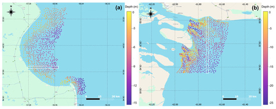
Figure 3.
Reference Bathymetric Data (RBD) for the study areas CA#1 (a) and CA#2 (b). The points within the white box were selected and excluded from the RBD to be used as an independent data test set (test bathymetric profile -TBP-).
2.4. Bathymetry Estimation Process
2.4.1. Alignment
The two sets of images (i.e., HSI and Ps-HSI) were aligned to the RBD using Euclidean distance. Therefore, two datasets of 870 (CA#1) and 1285 (CA#2) samples, each with 66 descriptors (i.e., ID, latitude, longitude, digital number of 63 bands), were created.
2.4.2. Data Splitting
Out of RDB, 7% (CA#1) and 5% (CA#2) were selected in order to get an independent bathymetric profile (herein called Test Bathymetric Profile -TBP-) across the complete depth range aimed to be tested (Figure 1 and Figure 3). The remaining RBD (i.e., 93% -CA#1- and 95% -CA#2-) were randomly split into 80%/20% for training and testing, respectively, where the former subset (i.e., training dataset -80%-) was, in turn, split into 80%/20% for training and validation, respectively (Figure 1 and Figure 3); a cross-validation was performed to investigate the ability of the four models. After the training, final accuracy assessment of the models was conducted employing both TBP and random test data (Figure 1 and Figure 3).
2.4.3. Standardization
To avoid biases caused by differences in properties (scale, units) of the descriptors, it is common to standardize the data. In this study, the Z-score standardization technique was adopted prior to the training procedure (Figure 1c), applying the usual formula:
where x represents the descriptors (see Section 2.4.1) corresponding to each reference point, and and represent the mean and standard deviation of the train + validation reference points (reference points used for testing are left out).
2.4.4. Band Optimization
Our study aimed to reduce redundancy in the hyperspectral data and to identify the most informative subset of bands for bathymetry estimation. To this end, a structured band optimization procedure was carried out. The procedure was designed to balance two objectives: minimizing the number of input bands while retaining the predictive accuracy of the models. The proposed method is illustrated in Figure 1b. First, a Random Forest (RF) regressor was trained using the full set of available hyperspectral bands from the training dataset, with bathymetric depth as the target variable. This model served as a baseline to capture nonlinear relationships between spectral signatures and depth.
Then, to quantify the relative contribution of each spectral band, the SHapley Additive exPlanations (SHAP) was applied, which is a model-agnostic interpretability method that decomposes predictions into feature-level attributions by calculating Shapley’s values from coalition game theory [31]. For every band, the absolute SHAP values were averaged across all training samples to yield a global measure of feature importance. Summing these values over all bands produced the Global Importance Factor (GIF-SHAP), which represents the total explanatory contribution of the spectral dataset. The bands were then ranked according to their SHAP importance values. To identify optimal subsets, an ablation strategy was applied. Starting from the full ranked list, the least important bands were progressively removed, and the cumulative importance (expressed as a fraction of the GIF-SHAP) at each stage was computed. Candidate subsets were generated corresponding to thresholds ranging from 100% down to 50% of the total importance, effectively producing nested sets of bands that retained only the most influential portions of the spectrum. For each candidate subset, the RF model was retrained and evaluated using independent validation data. Model performance was tracked in terms of , MAE, and RMSE.
The optimal subset of bands was defined as the smallest set that preserved model accuracy at a level comparable to or better than the full-band baseline. The resulting optimized datasets were called band optimized hyperspectral imagery (BoHSI) and band optimized pansharpened hyperspectral imagery (BoPsHSI). These datasets were subsequently used as inputs to the BoCNN and BoPsCNN models, respectively (Figure 1c).
2.4.5. 1D-CNN Model
CNNs are widely used in machine learning for automatic feature extraction and nonlinear representation learning [32]. In this study, a 1D-CNN architecture was implemented to model bathymetric depth from spectral descriptors. Compared to conventional 2D-CNNs, 1D-CNNs are computationally lighter and well-suited to one-dimensional spectral signals, achieving high performance with reduced model complexity [33,34,35].
The proposed 1D-CNN architecture consists of three convolutional blocks followed by a fully connected regression block (Figure 4). The network input is defined as a tensor of size N samples ×N descriptors (see Section 2.4.1), and the output layer predicts the corresponding depth values.
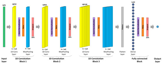
Figure 4.
Architecture of the proposed 1D-CNN model: The network consists of three consecutive 1D convolutional blocks. Each block has the following sequence: a input layer (green), a 1D convolutional layer (yellow), batch normalization layer (purple), ReLU activation layer (orange), a max-pooling layer (blue), and dropout layer (pink). Convolutional layers in each block increase the number of filters from 32 in block 1, to 64 in block 2, to 128 in block 3, with kernel sizes (k) alternating between 1 × 3 and 1 × 2 for convolution and pooling, respectively. The extracted feature maps are then flattened and passed through a fully connected block with a dense layer with 64 units, followed by batch normalization, ReLU activation, and a dropout layer. The final output layer produces the model predictions.
Each convolutional block includes a 1D convolution layer, batch normalization, ReLU activation, max pooling, and (in the first two blocks) dropout. The number of filters increases progressively (32, 64, and 128) with a kernel size of 3, balancing expressiveness and computational cost. Max pooling with a kernel size of 2 halves the feature dimension, improving efficiency and generalization. Dropout rates were set to 20% for convolutional and 10% for fully connected layers to prevent overfitting [36].
After the third block, feature maps are flattened and passed to a dense layer of 64 units with batch normalization, ReLU activation, and dropout. This fully connected block performs the regression task, producing the predicted depth. The model was trained using the Huber loss [37]:
The Huber loss combines the sensitivity of MSE to small errors with the robustness of MAE to large deviations, leading to stable convergence. The learning rate was initialized at 0.01 and reduced by 25% every 50 epochs, promoting rapid early learning and fine-tuning in later stages. Early stopping with a patience of 500 epochs was applied to prevent overfitting.
All models were implemented in Python 3.9 using the TensorFlow framework. To train and validate the model, four distinct input tensors were generated based on descriptors (see Section 2.4.1) extracted from each of the four datasets: HSI, Ps-HSI, BoHSI, and BoPsHSI. The reference depth points serve as labels for model training. A distinct model was trained and validated for each tensor, which is designated by the name of the respective tensor as follows: CNN, PsCNN, BoCNN, and BoPsCNN (see Figure 1c). This facilitated the evaluation of network performance across several dataset configurations.
2.5. 1D-CNN Models Validation and Testing
The validation of the 1D-CNN models (i.e., CNN, PsCNN, BoCNN, and BoPsCNN) during training was carried out by applying Equation (6), which involves MAE and MSE. The testing of the 1D-CNN models was made through the use of , MAE, and RMSE.
2.6. Computational Cost
The computational cost, among other things, depends on the dimension of the input dataset (i.e., spatial resolution and number of spectral bands). The runtime of each 1D-CNN model (for one scene) was calculated on the basis of a workstation equipped with an Intel® Core™ i7-12700H processor (2.30 GHz) and 32 GB of RAM. The massive data (millions of pixels) leads to dividing the dataset into blocks defined by the batch size parameter, thereby avoiding overload. For the runtime comparison, the time saving factor () was calculated as follows [38]:
where represents the execution time of the model with all bands, and represents the execution time of the model with optimization bands.
2.7. Derived Maps
Once tested, the bathymetric models aimed to derive reliable results, and the mapping can be built. Therefore, for each scene, the data were processed as follows:
- (a)
- Selection of the desired model (i.e., with or without pansharpening and with or without band optimization).
- (b)
- Data structuring: ID, latitude and longitude, and digital number are assigned for each pixel. It should be mentioned that the geographical coordinates of the Ps dataset are those of the panchromatic image.
- (c)
- Standardization: each data structured to be processed must be standardized using Equation (5).
- (d)
- Bathymetry prediction and mapping.
3. Results and Discussion
3.1. Reflectance Spectra in Shallow Waters
Reflectance spectra involve valuable information on the water constituents [39]. The average VNIR reflectance spectra of the sea water at three different depth zones for the two study areas (CA#1 and CA#2) and for the two datasets (HSI and PsHSI) are shown in Figure 5. Also, the standard deviation was plotted for the HSI dataset. In general terms, the reflectance peaks were observed in the spectral range from 400 to 700 nm in almost all cases. At longer wavelengths, the reflectance exhibited different trends. In the case of CA#1, the reflectance at low depth zone showed a remarkable increase in the range of approximately 700 to 900 nm for the HSI dataset (Figure 5a) due to the presence of a turbidity plume close to the coast, as was outlined in previous studies [25,26].
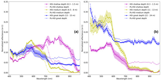
Figure 5.
VNIR reflectance spectra of HSI and Ps-HSI imagery at different depth zones for CA#1 (a) and CA#2 (b) study areas.
3.2. Band Optimization in Hyperspectral Imagery
As a result of the procedure described in Figure 1b, the best spectral bands for each study area are shown in Figure 6. The length of each bar is the absolute average of the SHAP value, indicating the magnitude of its influence on the predicted value. In CA#1, the most important bands are close to 700–850 nm, while in CA#2, the most important bands are close to 400–450 nm. Clearly, this difference in the best spectral bands should be attributed to the difference in reflectance spectra between CA#1 and CA#2, as shown in Figure 5. In addition, in CA#1, there is a notable difference in the most important spectral band for the two datasets (HSI and PsHSI), in accordance with the results of reflectance spectra in Figure 5a. Table 2 shows the assessment metrics for subsets of bands. As a result, the smallest optimal subset of bands capable of producing better performance is 38 and 24 bands for HSI and PsHSI datasets, respectively, in CA#1, and 37 and 36 bands for HSI and PsHSI datasets, respectively, in CA#2. Therefore, the number of bands is reduced to approximately half of its former number (i.e., 63).
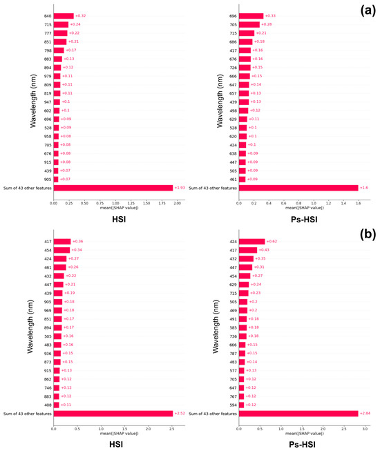
Figure 6.
Band optimization. SHAP plots showing the twenty most important spectral bands for the two datasets (HSI and Ps-HSI) for CA#1 (a) and CA#2 (b) study areas.
Table 2.
Band optimization. Assessment metrics for subsets of bands. Bold numbers indicate the best accuracy.
3.3. Bathymetry Estimation Using 1D-CNN
3.3.1. Testing of 1D-CNN Models on the Entire Study Area
The 1D-CNN model was applied to four testing datasets (i.e., HSI, Ps-HSI, BoHSI, and BoPsHSI) in order to predict four different bathymetric models (i.e., CNN, PsCNN, BoCNN, and BoPsCNN -Figure 1c-). Table 3 summarizes the details of the bathymetric models and the achieved assessment metrics. It was found that all these bathymetric models gave good results (Table 3, Figure 7).
Table 3.
Assessment metrics and band selection of the four 1D-CNN models (CNN, PsCNN, BoCNN, and BoPsCNN).
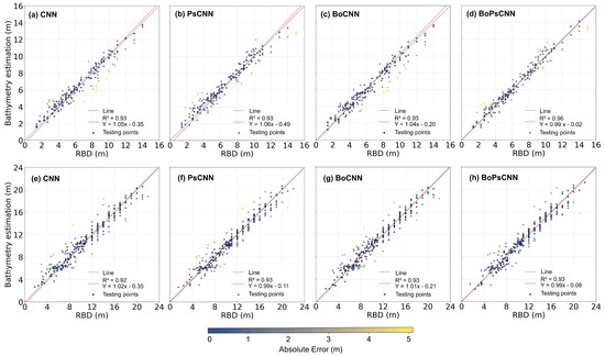
Figure 7.
Comparison of bathymetric estimations from the four 1D-CNN models (CNN, PsCNN, BoCNN, and BoPsCNN) against RBD corresponding to the testing dataset on the entire study area for CA#1 (a–d) and CA#2 (e–h). The red line (Y) shows the general trend of the model estimate versus the identity line (gray).
BoPsCNN produced slightly better results. For all models, the was greater than 0.92, varying slightly between 0.93 (BoCNN) and 0.96 (BoPsCNN) in CA#1 (Figure 7a–d) and between 0.92 (CNN) and 0.93 (PsCNN) in CA#2 (Figure 7e–h). The assessment of models regarding MAE gave values less than 1 m in all cases; BoPsCNN models gave the best MAE results, with values of 0.51 and 0.87 m in CA#1 and CA#2, respectively (Table 3). However, a few undesired predicted depths were identified, with absolute errors up to 5 m (Figure 7).
Some errors may be explained by spurious reflectivity in the sea surface (e.g., sunlight reflection). Although there seems to be no clear pattern of the above-mentioned errors, it can be noted that the models with pansharpening tended to increase the error in the shallowest and deepest zones (Figure 7). The latter is more pronounced in CA#1, where the presence of a narrow plume of turbidity at low depths might lead to prediction difficulties.
The variations of RMSE are similar to those of MAE, with values ranging between 0.65 (BoPsCNN) and 0.81 m (BoCNN) in CA#1 and between 1.16 (PsHSI) and 1.24 m (CNN) in CA#2 (Table 3).
3.3.2. Testing of 1D-CNN Models on a TBP
Additionally, the 1D-CNN models were tested on TBP in each study area (see Section 2.4.2 and Figure 3). Figure 8 shows the different 1D-CNN models along a profile involving a wide range of depths. As was expected, and in agreement with the above-mentioned results, the BoPsCNN model achieved the best performance results. Thus, the BoPsCNN had an of 0.95 (CA#1) and 0.92 (CA#2); the MAE and RMSE were 0.29 and 0.39 m, respectively, in CA#1, and 0.74 and 0.79 m, respectively, in CA#2. The BoCNN model also showed a good predictive performance (Figure 8). These results are comparable to those previously reported by Xi et al. [22], which obtained best RMSE values ranging from 0.82 to 1.43 m (at depths up to 25 m) by using PRISMA imagery and LSTM with an optimized bands model. On the other hand, as can be seen in Figure 8, the major prediction errors often occurred at greater depths in both study areas. In deeper zones, the best models predicted values slightly lower than RBD, indicating that the optical remote sensing reached its maximum effectiveness.
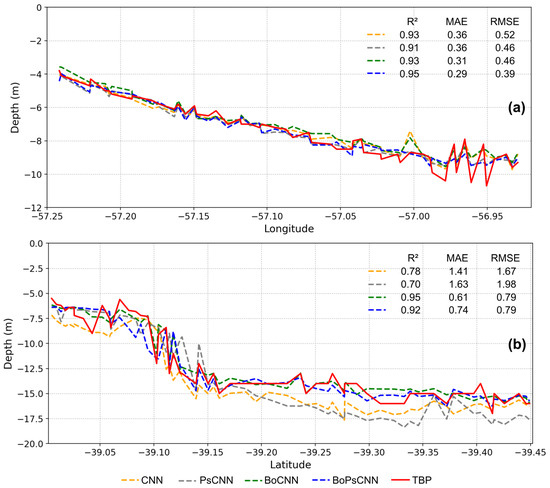
Figure 8.
Comparison of bathymetric estimations from the four 1D-CNN models (CNN, PsCNN, BoCNN, and BoPsCNN) against RBD corresponding to TBP for CA#1 (a) and CA#2 (b) study areas.
3.4. Computational Cost Assessment
The computational cost was evaluated for the four 1D-CNN models on one scene. Table 4 shows the computational cost details and results in both study areas. Basically, the runtime performance is congruent with the configurations of the models based on the spatial resolution (i.e., with and without pansharpening) and on the number of spectral bands (i.e., with and without band optimization). Thus, the PsCNN model displayed the maximum runtime (72 -CA#1- and 73 min -CA#2-), while in contrast, the BoCNN model displayed the minimum runtime (2 -CA#1- and 2.3 min -CA#2-) (Table 4). The application of band optimization meant a time-saving factor of about 33–36% when comparing models without pansharpening and of about 31–38% when comparing models with pansharpening (Table 4).
Table 4.
Computational cost of the four 1D-CNN models (CNN, PsCNN, BoCNN, and BoPsCNN) measured on one scene and implemented over an Intel® Core™ i7-12700H processor (2.30 GHz) and 32 GB of RAM. T: Time saving factor.
3.5. Bathymetry Mapping from 1D-CNN
The bathymetry mapping generated from the four 1D-CNN models is shown in Figure 9. It should be mentioned that the bathymetric mapping for the entire study area was presented forming a mosaic of bathymetric estimations corresponding to each scene, without the use of image processing techniques such as fusion and interpolation between two consecutive scenes.
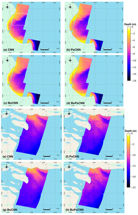
Figure 9.
Bathymetric maps generated from the four 1D-CNN models (CNN, PsCNN, BoCNN, and BoPsCNN) for CA#1 (a–d) and CA#2 (e–h) study areas. The white box (in capture (a)) indicates the reference capture used for scale analysis (see Figure 10).
Firstly, the bathymetry mapping of all models displayed gradual deepening from nearshore to offshore, which is consistent with the RBD. In general, the shape and texture of the seabed were found to be realistic in geomorphological terms. The latter is especially evident in models with pansharpening (i.e., PsCNN and BoPsCNN). Thus, for instance, in CA#1, long extended sand banks close to the coast were identified, in agreement with the study of Hausstein [40], who described this area as a “sediment trap” (Figure 9a). However, some isolated regions showed sudden changes which are related to the contact region of two consecutive scenes. The presence of different temporal data can imply the existence of differences in pixel reflectivity as well as in depth due to the adjustment procedures (e.g., tide level). In CA#2, the complex system of tidal courses (i.e., channels) of the Bahía Blanca estuary [41] was well represented in the west edge (Figure 9b).
Figure 10 shows the bathymetric maps from the 1D-CNN models for different zoom levels in a portion of the CA#1 study area. Also, testing values were considered. A great predictive capacity was observed in maps with pansharpening (i.e., PsCNN and BoPsCNN). The map derived from the BoPsCNN model presented the lowest error value, reaching a RMSE of 0.68 m. These maps are able to properly discriminate minor features due to their high spatial resolution (5 m/pixel) (Figure 10b,d). At these large scale detail levels, and from a visual analysis, the sea bottom displays lower contrast in the depths in maps with pansharpening, showing reliable performance; the depth range is slightly smaller in maps with pansharpening than in those without (Figure 10).

Figure 10.
Comparison of 1D-CNN models (CNN, PsCNN, BoCNN, and BoPsCNN) prediction at two different scales on a capture of study area CA#1 (see Figure 9). The white box indicates the zoom area. The green symbols show the reference bathymetric points. AE: absolute error.
4. Conclusions
The application of machine or deep learning algorithms for bathymetric estimation from hyperspectral imagery remains an emerging field of research. This novelty underscores the necessity for further methodological refinements and rigorous validation to enhance accuracy and reliability. We introduced an innovative methodology for bathymetric mapping in shallow coastal waters using a 1D-CNN applied to PRISMA hyperspectral imagery, with the dual objectives of improving mapping accuracy and optimizing computational efficiency. Four different 1D-CNN models were developed and evaluated in two study areas (CA#1 and CA#2) located in the Argentine sea, with performance assessments conducted against reference bathymetry data obtained from official nautical charts provided by the SHN.
The methodology provides the potential of combining 1D-CNN models with pansharpening and band optimization methods, yielding an efficient pipeline for high resolution shallow water bathymetric mapping. According to the test results, the BoPsCNN model achieved the best performance, which had an of 0.96 (CA#1) and 0.92 (CA#2); the MAE and RMSE were 0.29 and 0.39 m, respectively, in CA#1, and 0.74 and 0.79 m, respectively, in CA#2. The band optimization implementation reduced computational requirements by 31–38%, demonstrating substantial efficiency gains.
The bathymetric maps generated by the four 1D-CNN models consistently reproduced the expected depth gradient from nearshore to offshore zones while adequately resolving seabed morphologies. This fidelity was particularly evident in models incorporating pansharpened datasets (PsCNN and BoPsCNN). Improvements in future bathymetric investigations may come from the use of more and/or better reference data. Further studies will be focused on assessing the potential of the BoPsCNN model in different shallow coastal environments. In addition, the generalization ability of the proposed methodology can be further enhanced by integrating it with physically based radiative transfer models.
Author Contributions
Conceptualization, S.M.V., A.J.V. and C.A.D.; methodology, S.M.V.; software, S.M.V.; validation, S.M.V., S.A.G. and A.J.V.; formal analysis, S.M.V., S.A.G. and A.J.V.; investigation, S.M.V., S.A.G., A.J.V. and C.A.D.; resources, S.M.V., A.J.V. and C.A.D.; data curation, S.M.V., S.A.G. and A.J.V.; writing—original draft preparation, S.A.G.; writing—review and editing, S.M.V., S.A.G., A.J.V. and C.A.D.; visualization, S.M.V.; supervision, A.J.V. and C.A.D. All authors have read and agreed to the published version of the manuscript.
Funding
This research received no external funding.
Data Availability Statement
The PRISMA hyperspectral images are available from https://prisma.asi.it/ (accessed on 8 March 2024). The nautical charts are available from https://www.hidro.gov.ar/ (accessed on 8 March 2023).
Acknowledgments
The authors would like to thank the Italian Space Agency for allowing us access to the PRISMA hyperspectral imagery.
Conflicts of Interest
The authors declare no conflicts of interest.
References
- Ashphaq, M.; Srivastava, P.K.; Mitra, D. Review of near-shore satellite derived bathymetry: Classification and account of five decades of coastal bathymetry research. J. Ocean Eng. Sci. 2021, 6, 340–359. [Google Scholar] [CrossRef]
- Li, S.; Su, D.; Yang, F.; Zhang, H.; Wang, X.; Guo, Y. Bathymetric LiDAR and multibeam echo-sounding data registration methodology employing a point cloud model. Appl. Ocean Res. 2022, 123, 103147. [Google Scholar] [CrossRef]
- Su, D.; Yang, F.; Ma, Y.; Zhang, K.; Huang, J.; Wang, M. Classification of coral reefs in the South China Sea by combining airborne LiDAR bathymetry bottom waveforms and bathymetric features. IEEE Trans. Geosci. Remote Sens. 2019, 57, 815–828. [Google Scholar] [CrossRef]
- Guo, K.; Li, Q.; Mao, Q.; Wang, C.; Zhu, J.; Liu, Y.; Xu, W.; Zhang, D.; Wu, A. Errors of Airborne Bathymetry LiDAR Detection Caused by Ocean Waves and Dimension-Based Laser Incidence Correction. Remote Sens. 2021, 13, 1750. [Google Scholar] [CrossRef]
- Paterson, I.L.R.; Dawson, K.E.; Mogg, A.O.M.; Sayer, M.D.J.; Burdett, H.L. Quantitative comparison of ROV and diver-based photogrammetry to reconstruct maerl bed ecosystems. Aquat. Conserv. Mar. Freshw. Ecosyst. 2024, 34, 103147. [Google Scholar] [CrossRef]
- Raber, G.T.; Schill, S.R. Reef Rover: A Low-Cost Small Autonomous Unmanned Surface Vehicle (USV) for Mapping and Monitoring Coral Reefs. Drones 2019, 3, 38. [Google Scholar] [CrossRef]
- Hatcher, G.A.; Warrick, J.A.; Ritchie, A.C.; Dailey, E.T.; Zawada, D.G.; Kranenburg, C.; Yates, K.K. Accurate Bathymetric Maps From Underwater Digital Imagery Without Ground Control. Front. Mar. Sci. 2020, 7, 525. [Google Scholar] [CrossRef]
- Jin, J.; Zhang, J.; Shao, F.; Lyu, Z.; Wang, D. A novel ocean bathymetry technology based on an unmanned surface vehicle. Acta Oceanol. Sin. 2018, 37, 99–106. [Google Scholar] [CrossRef]
- Genchi, S.A.; Vitale, A.J.; Perillo, G.M.E.; Seitz, C.; Delrieux, C.A. Mapping Topobathymetry in a Shallow Tidal Environment Using Low-Cost Technology. Remote Sens. 2020, 12, 1394. [Google Scholar] [CrossRef]
- Martínez Vargas, S.; Vitale, A.J.; Genchi, S.A.; Nogueira, S.F.; Arias, A.H.; Perillo, G.M.E.; Siben, A.; Delrieux, C.A. Monitoring multiple parameters in complex water scenarios using a low-cost open-source data acquisition platform. HardwareX 2023, 16, e00492. [Google Scholar] [CrossRef]
- Li, Z.; Peng, Z.; Zhang, Z.; Chu, Y.; Xu, C.; Yao, S.; García-Fernández, Á.F.; Zhu, X.; Yue, Y.; Levers, A.; et al. Exploring modern bathymetry: A comprehensive review of data acquisition devices, model accuracy, and interpolation techniques for enhanced underwater mapping. Front. Mar. Sci. 2023, 10, 1178845. [Google Scholar] [CrossRef]
- Li, X.; Yang, X.; Zheng, Q.; Pietrafesa, L.J.; Pichel, W.G.; Li, Z.; Li, X. Deep-water bathymetric features imaged by spaceborne SAR in the Gulf Stream region. Geophys. Res. Lett. 2010, 37, L19603. [Google Scholar] [CrossRef]
- Martínez Vargas, S.; Delrieux, C.; Blanco, K.L.; Vitale, A.J. Dense Bathymetry in Turbid Coastal Zones Using Airborne Hyperspectral Images. Photogramm. Eng. Remote Sens. 2021, 87, 923–927. [Google Scholar] [CrossRef]
- Lyzenga, D.R. Passive remote sensing techniques for mapping water depth and bottom features. Appl. Opt. 1978, 17, 379–383. [Google Scholar] [CrossRef]
- Dierssen, H.M.; Theberge, A.E., Jr. Bathymetry: Assessing Methods. In Encyclopedia of Natural Resources, Vol. II—Water and Air; Taylor & Francis: Boca Raton, FL, USA, 2014; pp. 1–8. [Google Scholar] [CrossRef]
- Sun, S.; Chen, Y.; Mu, L.; Le, Y.; Zhao, H. Improving shallow water bathymetry inversion through nonlinear transformation and deep convolutional neural networks. Remote Sens. 2023, 15, 4247. [Google Scholar] [CrossRef]
- Xie, C.; Chen, P.; Zhang, S.; Huang, H. Nearshore Bathymetry from ICESat-2 LiDAR and Sentinel-2 Imagery Datasets Using Physics-Informed CNN. Remote Sens. 2024, 16, 511. [Google Scholar] [CrossRef]
- Xu, Q.; Zhang, Y.; Li, B. Recent advances in pansharpening and key problems in applications. Int. J. Remote Sens. 2014, 35, 175–195. [Google Scholar] [CrossRef]
- Loncan, L.; Almeida, L.B.; Bioucas-Dias, J.M.; Briottet, X.; Chanussot, J.; Dobigeon, N.; Fabre, S.; Liao, W.; Licciardi, G.A.; Simoes, M.; et al. Hyperspectral pansharpening: A review. IEEE Geosci. Remote Sens. Mag. 2015, 3, 27–46. [Google Scholar] [CrossRef]
- Karimi, D.; Kabolizadeh, M.; Rangzan, K.; Zaheri Abdehvand, Z.; Balouei, F. New methodology for improved bathymetry of coastal zones based on spaceborne spectroscopy. Int. J. Environ. Sci. Technol. 2025, 22, 3359–3378. [Google Scholar] [CrossRef]
- Qi, J.; Gong, Z.; Yao, A.; Liu, X.; Li, Y.; Zhang, Y.; Zhong, P. Bathymetric-Based Band Selection Method for Hyperspectral Underwater Target Detection. Remote Sens. 2021, 13, 3798. [Google Scholar] [CrossRef]
- Xi, X.; Chen, M.; Wang, Y.; Yang, H. Band-Optimized Bidirectional LSTM Deep Learning Model for Bathymetry Inversion. Remote Sens. 2023, 15, 3472. [Google Scholar] [CrossRef]
- Wang, Y.; Chen, M.; Xi, X.; Yang, H. Bathymetry Inversion Using Attention-Based Band Optimization Model for Hyperspectral or Multispectral Satellite Imagery. Water 2023, 15, 3205. [Google Scholar] [CrossRef]
- Servicio de Hidrografía Naval (SHN). Sitio Web Oficial. Available online: https://www.hidro.gov.ar/ (accessed on 21 July 2025).
- Dogliotti, A.I.; Ruddick, K.G.; Guerrero, R.A. Seasonal and inter-annual turbidity variability in the Río de la Plata from 15 years of MODIS: El Niño dilution effect. Estuar. Coast. Shelf Sci. 2016, 182, 27–39. [Google Scholar] [CrossRef]
- Framiñán, M.B.; Brown, O.B. Study of the Río de la Plata turbidity front, Part 1: Spatial and temporal distribution. Cont. Shelf Res. 1996, 16, 1259–1282. [Google Scholar] [CrossRef]
- Arena, M.; Pratolongo, P.; Loisel, H.; Tran, M.D.; Jorge, D.S.F.; Delgado, A.L. Optical Water Characterization and Atmospheric Correction Assessment of Estuarine and Coastal Waters around the AERONET-OC Bahía Blanca. Front. Remote Sens. 2024, 5, 1305787. [Google Scholar] [CrossRef]
- Sharma, K.V.; Kumar, V.; Singh, K.; Mehta, D.J. LANDSAT 8 LST Pan sharpening using novel principal component based downscaling model. Remote Sens. Appl. Soc. Environ. 2023, 30, 100963. [Google Scholar] [CrossRef]
- Vivone, G.; Restaino, R.; Dalla Mura, M.; Chanussot, J. Multi-band semiblind deconvolution for pansharpening applications. In Proceedings of the IEEE International Geoscience and Remote Sensing Symposium (IGARSS 2015), Milan, Italy, 26–31 July 2015; IEEE: Piscataway, NJ, USA, 2015; pp. 41–44. [Google Scholar] [CrossRef]
- QGIS Development Team QGIS Geographic Information System. Open Source Geospatial Foundation Project. Available online: http://qgis.org (accessed on 21 July 2025).
- Shapley, L.S. A Value for n-Person Games. In Contributions to the Theory of Games, Volume II; Kuhn, H.W., Tucker, A.W., Eds.; Princeton University Press: Princeton, NJ, USA, 1953; pp. 307–318. [Google Scholar] [CrossRef]
- Eren, L. Bearing Fault Detection by One-Dimensional Convolutional Neural Networks. Math. Probl. Eng. 2017, 2017, 8617315. [Google Scholar] [CrossRef]
- Escottá, Á.T.; Beccaro, W.; Arjona Ramírez, M.A. Evaluation of 1D and 2D deep convolutional neural networks for driving event recognition. Sensors 2022, 22, 4226. [Google Scholar] [CrossRef]
- Qazi, E.U.H.; Almorjan, A.; Zia, T. A One-Dimensional Convolutional Neural Network (1D-CNN) Based Deep Learning System for Network Intrusion Detection. Appl. Sci. 2022, 12, 7986. [Google Scholar] [CrossRef]
- Kiranyaz, S.; Avci, O.; Abdeljaber, O.; Ince, T.; Gabbouj, M.; Inman, D.J. 1D convolutional neural networks and applications: A survey. Mech. Syst. Signal Process. 2021, 151, 107398. [Google Scholar] [CrossRef]
- Chai, E.; Pilanci, M.; Murmann, B. Separating the Effects of Batch Normalization on CNN Training Speed and Stability Using Classical Adaptive Filter Theory. arXiv 2020, arXiv:2002.10674. [Google Scholar] [CrossRef]
- Hastie, T.; Tibshirani, R.; Friedman, J. The Elements of Statistical Learning: Data Mining, Inference, and Prediction, 2nd ed.; Springer Series in Statistics; Springer: New York, NY, USA, 2009; ISBN 978-0-387-84857-0. [Google Scholar] [CrossRef]
- Park, J.; Lee, J.; Sim, D. Low-complexity CNN with 1D and 2D filters for super-resolution. J. Real-Time Image Process. 2020, 17, 2065–2076. [Google Scholar] [CrossRef]
- Gordon, H.R.; Brown, O.B.; Evans, R.H.; Brown, J.W.; Smith, R.C.; Baker, K.S.; Clark, D.K. A semianalytic radiance model of ocean color. J. Geophys. Res. Atmos. 1988, 93, 10909–10924. [Google Scholar] [CrossRef]
- Hausstein, H. Simulation of the Transport of Suspended Particulate Matter in the Río de la Plata; GKSS 2008/7; GKSS Research Centre: Geesthacht, Germany, 2008. [Google Scholar]
- Perillo, G.M.E.; Piccolo, M.C.; Parodi, E.; Freije, R.H. The Bahía Blanca Estuary, Argentina. In Coastal Marine Ecosystems of Latin America; Seeliger, U., Kjerfve, B., Eds.; Springer: Berlin/Heidelberg, Germany, 2001; pp. 205–217. [Google Scholar] [CrossRef]


Disclaimer/Publisher’s Note: The statements, opinions and data contained in all publications are solely those of the individual author(s) and contributor(s) and not of MDPI and/or the editor(s). MDPI and/or the editor(s) disclaim responsibility for any injury to people or property resulting from any ideas, methods, instructions or products referred to in the content. |
© 2025 by the authors. Licensee MDPI, Basel, Switzerland. This article is an open access article distributed under the terms and conditions of the Creative Commons Attribution (CC BY) license (https://creativecommons.org/licenses/by/4.0/).