Article

Phenology-Guided Wheat and Corn Identification in Xinjiang: An Improved U-Net Semantic Segmentation Model Using PCA and CBAM-ASPP

1
School of Architecture and Civil Engineering, Chengdu University, Chengdu 610106, China
2
School of Earth Resources, China University of Geosciences, Wuhan 430074, China
*
Author to whom correspondence should be addressed.
Remote Sens. 2025, 17(21), 3563; https://doi.org/10.3390/rs17213563
Submission received: 23 August 2025 / Revised: 18 October 2025 / Accepted: 23 October 2025 / Published: 28 October 2025

Highlights

What are the main findings?
  • By analysing kNDVI/EVI time-series vegetation indices via GEE, this study identifies days 156–176 of the year as the optimal window for wheat and corn identification, effectively eliminating spectral similarity interference.
  • An improved U-Net model integrated with ResNet50, CBAM, and a modified ASPP module achieves outstanding performance (mIoU of 83.03% and OA of 90.91%) on PCA-dimensionally reduced Sentinel-2 data, outperforming mainstream models like DeeplabV3+ and PSPnet.
What is the implication of the main finding?
  • The PCA-constructed dataset supplements the spectral information that is missing in traditional RGB data, and when combined with the optimal time window and improved model, forms a complete “time series + data + model” technical path for accurate crop identification.
  • The model exhibits strong generalization (error < 2% in Qitai County, Xinjiang) and can be extended to arid grain-producing areas for crop mapping, calculating area statistics, and yield estimation, providing practical support for national food security.

Abstract

Wheat and corn are two major food crops in Xinjiang. However, the spectral similarity between these crop types and the complexity of their spatial distribution has posed significant challenges to accurate crop identification. To this end, the study aimed to improve the accuracy of crop distribution identification in complex environments in three ways. First, by analysing the kNDVI and EVI time series, the optimal identification window was determined to be days 156–176—a period when wheat is in the grain-filling to milk-ripening phase and maize is in the jointing to tillering phase—during which, the strongest spectral differences between the two crops occurs. Second, principal component analysis (PCA) was applied to Sentinel-2 data. The top three principal components were extracted to construct the input dataset, effectively integrating visible and near-infrared band information. This approach suppressed redundancy and noise while replacing traditional RGB datasets. Finally, the Convolutional Block Attention Module (CBAM) was integrated into the U-Net model to enhance feature focusing on key crop areas. An improved Atrous Spatial Pyramid Pooling (ASPP) module based on deep separable convolutions was adopted to reduce the computational load while boosting multi-scale context awareness. The experimental results showed the following: (1) Wheat and corn exhibit obvious phenological differences between the 156th and 176th days of the year, which can be used as the optimal time window for identifying their spatial distributions. (2) The method proposed by this research had the best performance, with its mIoU, mPA, F1-score, and overall accuracy (OA) reaching 83.03%, 91.34%, 90.73%, and 90.91%, respectively. Compared to DeeplabV3+, PSPnet, HRnet, Segformer, and U-Net, the OA improved by 5.97%, 4.55%, 2.03%, 8.99%, and 1.5%, respectively. The recognition accuracy of the PCA dataset improved by approximately 2% compared to the RGB dataset. (3) This strategy still had high accuracy when predicting wheat and corn yields in Qitai County, Xinjiang, and had a certain degree of generalisability. In summary, the improved strategy proposed in this study holds considerable application potential for identifying the spatial distribution of wheat and corn in arid regions.

1. Introduction

Against the backdrop of sustained global economic development and rapid population growth, precision agriculture has become a key component of sustainable development and modernisation in the 21st century [1,2]. Information on the spatial distribution of crops is the foundation of modern agriculture, and accurately obtaining information on the temporal and spatial distribution of crops is an important challenge in sustainable agriculture [3,4,5]. Wheat and corn are China’s highest-yielding grain crops [6], and Xinjiang is an important grain production base for wheat and corn in China, playing a vital role in ensuring national food security. Efficiently and accurately extracting crop planting information and predicting yields play a crucial role in preventing famine and ensuring food security [7,8].
Satellite remote sensing technology, which boasts advantages like a wide coverage and real-time monitoring capabilities [9], has gradually emerged as a core technology for countries and the Food and Agriculture Organisation of the United Nations (FAO) to monitor global crop growth and the planting conditions of various crops [7]. Wheat and corn are among the most widely cultivated cereal crops in the world and are also major staple foods in China [10,11,12]. However, due to the characteristics of these crops, which are widely distributed, scattered, and subject to large fluctuations in planting area [13,14], traditional remote sensing methods face many challenges in terms of identification accuracy due to the influence of spectral information and resolution.
In previous studies, machine learning algorithms have demonstrated significant advantages in tasks such as crop identification and extraction due to their powerful data processing and pattern recognition capabilities. For example, Immitzer et al. [15] utilised Sentinel-2 satellite data and combined it with techniques including Random Forest (RF) to generate detailed distribution maps of various crops and tree species in the states of Austria. However, this study relied solely on single-phase data and failed to fully utilise the crops’ phenological sequence characteristics, making it difficult to address crop confusion issues in complex cultivation environments. Qi et al. [16] employed machine learning to develop a process for extracting smallholder farming information, which provided technical support and a decision-making basis for accurately acquiring the spatio-temporal distribution of crops and optimising agricultural production. Nevertheless, its methodology relies on fixed-time point composite data from the Google Earth Engine platform and exhibits limited adaptability to optical data gaps caused by cloudy conditions in arid regions. Additionally, Wei et al. [17] utilised the Random Forest (RF) algorithm and Sentinel-2 time series data to investigate the earliest time that corn, wheat, and soybeans can be identified while also extracting crop information. However, this study focused on the humid and semi-humid climate zones of the Sanjiang Plain and failed to account for phenological shifts in arid regions caused by irrigation-regulated crop growth. Furthermore, traditional machine learning models struggle to capture the deep nonlinear spectral characteristics of crops. Hao et al. [18] combined MODIS time series of varying lengths with the RF algorithm to achieve accurate crop type classification in Kansas, USA. Although the data offered broad spatial coverage, using the 500-metre spatial resolution data, the algorithm struggled to meet the requirements for detailed identification at the plot scale. Yu et al. [19] integrated Sentinel-1 and Sentinel-2 time series data with multiple machine learning algorithms, realising precise crop classification in the arid region of the Sanhe Tun Irrigation District in Xinjiang. However, the traditional machine learning models employed in this study (RF, CART, and SVM) possess limited capability for feature selection in high-dimensional datasets. Furthermore, the model architecture was not optimised to account for the characteristics of crops in arid regions—such as wheat and maize—which feature short growing seasons and minimal spectral differences. Consequently, there remains room for improvement in terms of classification accuracy for certain similar crops.
The rapid evolution of deep learning has led to a growing adoption of semantic segmentation algorithms in tasks such as crop segmentation [20,21,22]. By combining deep learning with remote sensing technology, particularly using high-resolution remote sensing satellite data, it is possible to achieve precise segmentation of crop information and obtain more accurate spatial distribution information on crops [23,24]. Li et al. [25] introduced the U-Net model with an image pyramid structure, which showed significantly improved spatial feature learning capabilities and enabled the accurate extraction and mapping of citrus growing areas. Although the introduction of image pyramids and ASPP enhanced the model’s spatial feature extraction capabilities, addressing the issue of blurred extraction of irregular plots in traditional U-Net models, the feature extraction strategy remains unoptimised for spectral similarities between citrus and surrounding similar vegetation, such as tea plantations. Chang et al. [26] presented an improved DeepLabV3+ semantic segmentation model, which effectively improved the extraction accuracy for small crops in complex environments. Although the improved DeepLab3+ model reduced the scale of the model parameters and enhanced the recognition of small-area crops such as wheat and rapeseed, it does not account for the interference caused by soil backgrounds in arid regions that affects crop boundary identification. Bian et al. [27] proposed the CACPU-Net model based on Sentinel-2 autumn remote sensing data. By introducing an attention mechanism and designing modules focused on complex areas, they effectively improved the accuracy of crop identification in complex areas. The CACPU-Net model enhances the discriminative power of algorithms that compare crop spectral features, effectively addressing classification errors at field boundaries. However, this model relies on spectral differences during the autumn crop maturation season and does not account for variations arising from different crop growth cycles.
Currently, achieving accurate crop identification under complex environmental conditions remains a key issue in the application of deep learning to agricultural remote sensing. The crop planting structure in the Xinjiang region is complex, and the similarity of crop spectra is high, posing a significant challenge for deep learning crop identification. In this study, we first determined the optimal time window for identifying wheat and corn by integrating kNDVI and NDVI time-series features. Subsequently, we constructed a dataset by reducing the dimensionality through principal component analysis (PCA) and combined it with an improved U-Net semantic segmentation model to achieve accurate identification of wheat and corn in complex environments. This model avoided the gradient vanishing problem in deep networks by introducing ResNet50 as the main network. Simultaneously, it incorporates a deepwise separable Atrous Spatial Pyramid Pooling (ASPP) model. This component lowers the computational load and complexity during model training and enhances the model’s ability to extract contextual information. Furthermore, an attention mechanism called a Convolutional Block Attention Module (CBAM) was introduced to improve the feature extraction capabilities for key regions.
In summary, to address the challenge of accurately identifying wheat and corn in complex planting environments, this study developed a new method.
The core work and steps of this study were as follows:
(1)
Determine the optimal identification window: Time-series vegetation indices were utilised to analyse the phenological characteristics of wheat and corn, thereby identifying the optimal window period for their accurate recognition.
(2)
Construct a high-efficiency dataset: PCA was applied to reduce the dimensionality of Sentinel-2 remote sensing data. Key principal components were extracted from the dimensionality-reduced data to build the input dataset for the model.
(3)
Improve the U-Net model: A Convolutional Block Attention Module (CBAM) and an improved Atrous Spatial Pyramid Pooling (ASPP) module were integrated into the U-Net model. This enhancement enables the model to extract crop feature information more accurately and efficiently.
(4)
Apply the model for crop extraction: Based on the improved model, wheat and corn were extracted from Sentinel-2 images covering Qitai County, Xinjiang, China.

2. Research Area and Materials

2.1. Study Area

The study area is situated in Qitai County, Changji Hui Autonomous Prefecture, northeastern Xinjiang—specifically at the western foot of the Tianshan Mountains and the southeastern edge of the Junggar Basin (see Figure 1). It lies between 89°13′–91°22′E longitude and 42°25′–45°29′N latitude, with the northern foothills of Bogda Peak (eastern segment of the Tianshan Mountains) to its south and the Gurbantunggut Desert to its north. The terrain slopes from north to south, and the climate is classified as a temperate continental arid climate. The annual average precipitation is approximately 269 mm, with abundant sunshine and strong evaporation, resulting in annual sunshine hours exceeding 2500 h. The region experiences hot summers, cold winters, and significant diurnal temperature variations [28,29]. The main irrigated farmland consists of central plains and hills, and the main crops are wheat, corn, cotton, etc.
Table 1 presents the phenological calendars for spring wheat and corn, two major crops in this region. Spring wheat is sown in early April and matures in late July, with a growing season spanning April to July. Corn is sown in mid-April and matures in mid-September, with a growing season extending from April to September.

2.2. Data Sources and Preprocessing

The Sentinel-2 satellite remote sensing data used in this study was sourced from the Copernicus Data Space Ecosystem (ESC). The Sentinel-2 satellite can measure 13 optical spectral bands [30] with resolutions of 10 m, 20 m, and 60 m, and an orbital swath width of 290 km. This data is widely used in land use classification, crop information extraction, phenology, and other fields. To reduce the impact of weather conditions such as clouds and fog, data with a cloud cover exceeding 20% was not included in the calculations. Subsequently, atmospheric correction and band resampling (10 m) were performed using the Sen2Cor plugin [31]. Building upon this foundation, we employed ENVI4.8 to perform principal component analysis on the processed imagery. Subsequently, we selected the three most significant principal components—PCA1, PCA2, and PCA3—to constitute the principal component analysis dataset.

2.3. Dataset Construction

The actual ground truth data for the wheat and corn crops was obtained from field surveys conducted between April and August 2022. With the help of high-resolution images from Google Earth and Sentinel-2, the actual cultivation areas corresponding to each sample were manually outlined in QGIS3.34 software through visual interpretation. After atmospheric correction and resampling, the original images underwent PCA dimensionality reduction. The first three principal components (PCA1–PCA3) were selected as model inputs, replacing the original traditional RGB data. In order to adapt to the model’s input requirements, the image was cropped into 128 × 128-pixel samples. The overlap rate was set to 20% to reduce discontinuity at the boundaries. The dataset was then expanded using methods such as flipping and rotation to improve the model’s generalisation ability, resulting in a total of 9370 images, of which, 70% were used as the training set, 15% as the test set, and 15% as the validation set. All data samples in this experiment were collected within the 156- to 176-day time window when phenological differences were most pronounced, ensuring maximum spectral separability.

3. Methods

3.1. Time Series Reconstruction of Vegetation Indices

We leveraged the temporal features of vegetation indices to study the time window where the spectral differences between corn and wheat were the largest. Using the GEE platform, we calculated the Kndvi (kernel normalised difference vegetation index) and EVI (enhanced vegetation index) for the study area based on the Sentinel-2 dataset and plotted time-series vegetation index curves for wheat and maize separately. Subsequently, Savitzky–Golay (S-G) filtering was used to smooth and denoise the time series data in order to reduce the effects of clouds, snow, and other factors. The Savitzky–Golay time series filtering method uses a weighted average filter based on local polynomial regression and is widely used in the reconstruction of vegetation index time series. The pre-processed vegetation index smoothing curve was used as the basis for analysing the phenological characteristics of wheat and corn and identifying the optimal window period.
The Normalised Difference Vegetation Index (NDVI) is currently one of the most widely used vegetation indices. The index ranges from −1 to 1. The higher the value, the higher the vegetation coverage. A value of 0 or a negative value indicates the presence of bare soil, clouds, snow, etc. The formula for NDVI is
N D V I = N I R R e d N I R + R e d ,
In the formula, NIR refers to the near-infrared band and Red refers to the red light band.
Camp-Valls et al. [32] proposed a kernel normalised vegetation index (Kndvi) based on machine learning and improvements to kernel method theory. This index was more resistant to saturation, bias, and complex phenological cycles, making it more suitable for handling noise, saturation, and complex phenology [33,34]. The ease of calculation of this index makes it highly applicable to natural and agricultural systems. The formula for calculating Kndvi was as follows:
k N D V I = tanh N I R R e d 2 2 σ ,
In the formula, σ is a length scale parameter specified for each specific application, representing the sensitivity of the exponent to sparse/dense vegetation areas; NIR is the near-infrared band; red is the red light band; and tanh is the hyperbolic tangent function. The reasonable value of σ was the average of red and NIR, i.e., σ = 0.5 (NIR + red). The formula for Kndvi can be rewritten as
k N D V I = tanh ( N D V I ) 2 ,

3.2. Deep Learning Methods

3.2.1. Improving the U-Net Model

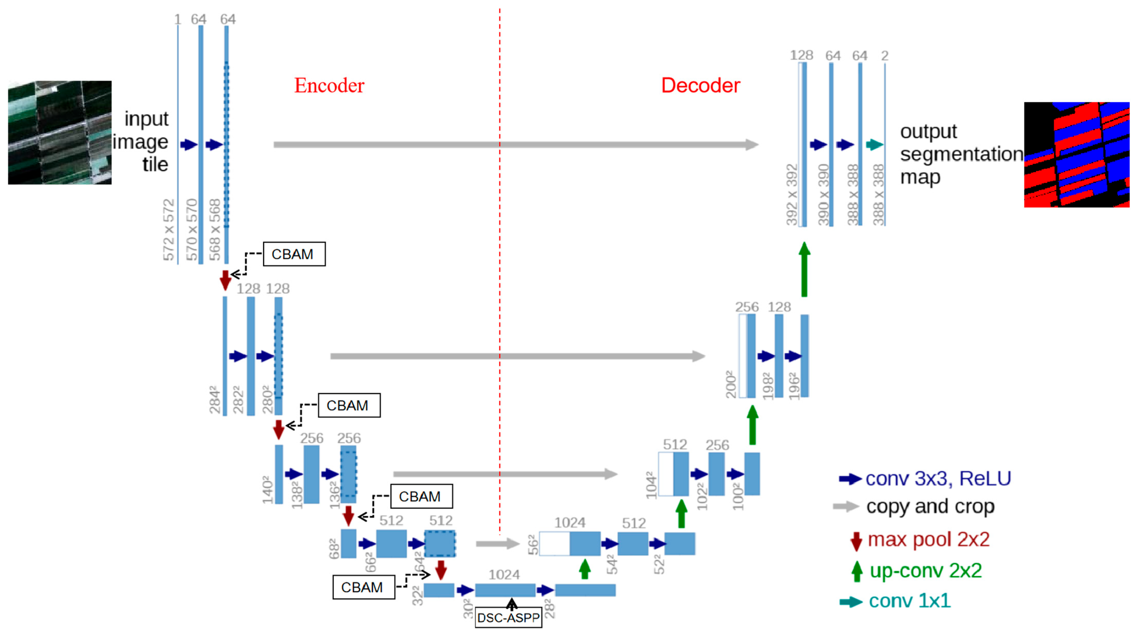
The U-Net model was first proposed by Ronneberger et al. [35] and has been widely used in medical image segmentation tasks due to its excellent performance. The network mainly consists of encoder and decoder structures. As the main feature, the encoder downsamples the input image through convolution and pooling, thereby capturing context features that are rich in semantic information. The decoder fuses images through skip connections and gradually restores them. Therefore, the U-Net network can produce fine segmentation results. However, in more complex scenarios such as remote sensing image segmentation tasks, the U-Net model finds it difficult to extract deeper information [36]. In order to make the model more suitable for remote sensing image segmentation tasks for wheat and corn identification, this study made the following improvements based on the U-Net model: First, we replaced the main feature extraction network with the Resnet50 model. This model solves the gradient vanishing problem in deep networks by introducing residual blocks. This enables the U-Net network to extract deeper and more detailed semantic segmentation information. Secondly, an ASPP module based on depth-separable convolutions was added between the encoder and decoder. This module enhances multi-scale feature extraction and context information fusion capabilities, which can improve segmentation performance. Finally, we added a normalisation layer after each convolution in the decoder. The input was adjusted to a normal distribution with a mean of 0 and a variance of 1 to avoid excessive data volume during pooling, which can cause network training instability, and accelerate model convergence. By incorporating the CBAM attention mechanism module into the downsampling layers of the model encoder, the network’s ability to focus on key regions of input targets and extract features is further enhanced while reducing interference from irrelevant information. This enables the model to more accurately capture critical semantic features and improve its processing capabilities to capture target details.

3.2.2. CBAM Attention Mechanism

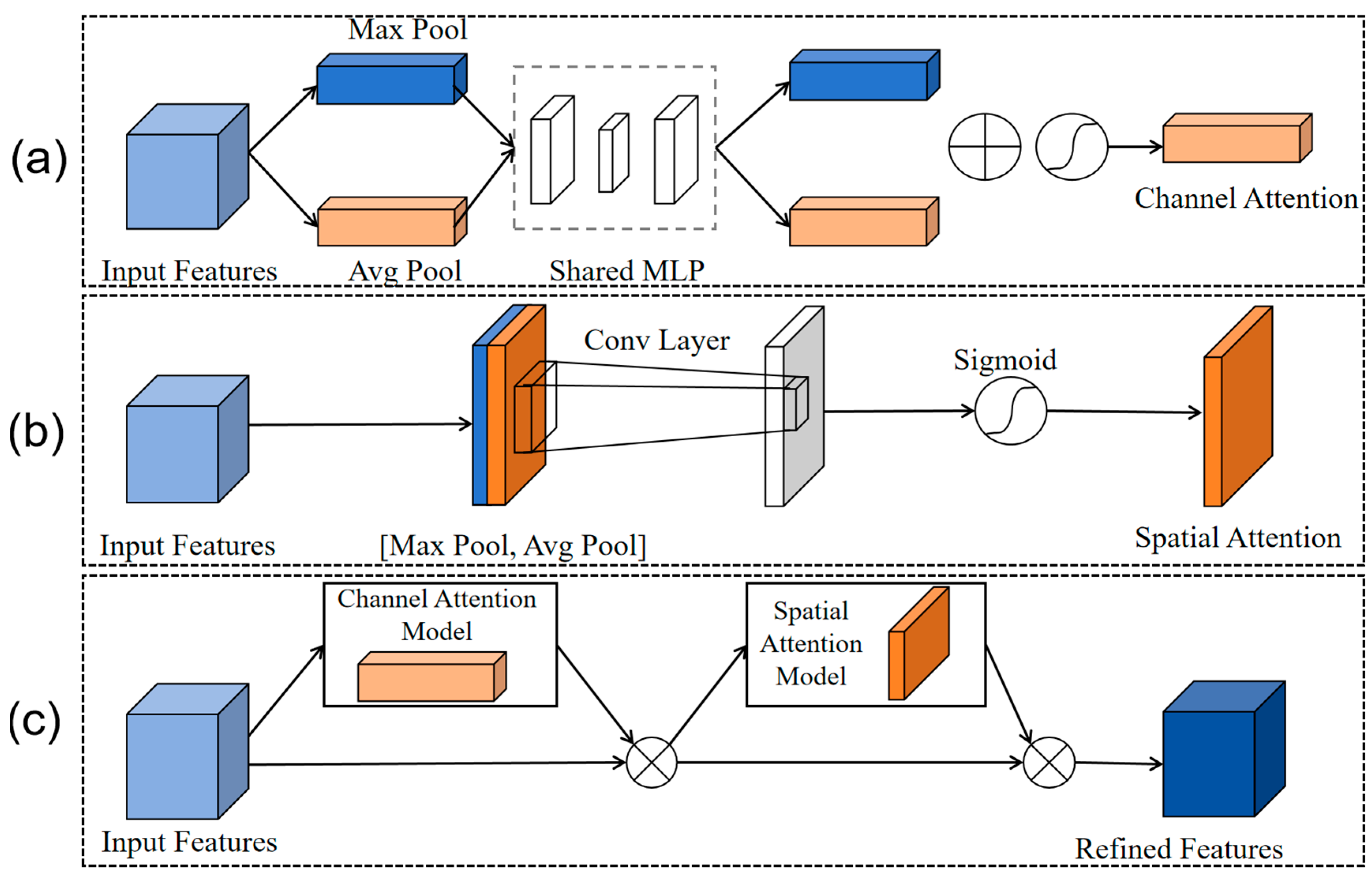
An attention mechanism is a method that simulates human visual attention, enabling the model to focus more on task-relevant areas during data processing. Introducing an attention mechanism can better capture useful feature information [37]. A CBAM is a simple and highly effective lightweight general-purpose attention module. It improves the performance of convolutional neural networks by combining channel attention mechanisms and spatial attention mechanisms (Figure 2). At the same time, this module also focuses on channel and spatial feature information to obtain more accurate results [38].
The channel attention mechanism structure model first performs max pooling and average pooling on the input feature maps to obtain the maximum and average values in the feature maps [39]. These are then fed into a multi-layer perceptron and the number of channels in the feature map are compressed. Finally, the output features are added element-wise and passed through a sigmoid activation function to obtain the channel attention feature map.
The spatial attention mechanism structure model takes the feature map obtained through the channel attention module as input and concatenates it after maximum pooling and average pooling. Then, it is converted into a single-channel feature map through a 7 × 7 convolution layer. Finally, the weights are obtained through the sigmoid activation function and multiplied by the input feature map to obtain the spatial attention feature map [39,40].

3.2.3. ASPP Model Based on Deep Separable Convolutions

In the ASPP module, the standard 3 × 3 convolution (Conv) is replaced with depthwise separable convolution. The depthwise convolution (DSConv) employs a 3 × 3 kernel with a group size equal to the number of input channels, extracting features channel-by-channel. This is followed by pointwise convolution (Pointwise Conv), i.e., a 1 × 1 standard convolution, which fuses the information from all the channels (Figure 3).
Depthwise separable convolution decomposes standard convolution into channel-wise convolution and point-wise convolution [41]. Channel-wise convolution performs convolution operations on each channel of the input to obtain feature maps with the same number of input channels. This operation allows the convolution operation to be performed independently on each channel of the input, thereby greatly reducing the amount of computation required. Point-wise convolution uses a 1 × 1 convolution kernel to perform a weighted combination operation on the feature map obtained in the previous step in the channel to generate the final feature map. The above operations can significantly reduce the number of parameters in the model while maintaining its performance, thereby improving the efficiency of model training. The ASPP model, or Atrial Space Pooling Pyramid model, consists of multiple sets of convolution operations and global average pooling operations. The input feature map is processed through a series of hollow convolutions with different expansion rates to capture feature information at different scales [42]. Then, global average pooling is used to extract contextual feature information and concatenate the information obtained from each layer. The dimension of the feature map is reduced to the required number of channels through a 1 × 1 convolution operation to obtain the final feature map. This study replaces the traditional standard convolution in the pattern replacement model with a combination of deep separable convolution and ASPP models. This structure is designed to reduce the number of computational parameters and complexity during model training, thereby improving the model’s feature extraction capabilities and training efficiency in segmentation tasks [43].

3.3. Training Experiment Parameter Settings

The experimental environment of this study utilised PyTorch (Python 3.10) as the deep learning development framework. The computer’s hardware configuration featured an Intel Core i7-12700F CPU (2.10 GHz) and an NVIDIA GeForce RTX 3070 GPU. Considering the computer’s configuration and resource constraints, the training parameters were configured as follows: batch size = 8, initial learning rate = 0.0001 (minimum learning rate = 0.01 × initial learning rate), Adam optimizer (momentum = 0.9), and cosine annealing algorithm for learning rate decay. The training process was run for 100 epochs. The specific model is shown in Figure 4. Additionally, a weighted cross-entropy function was used to calculate the loss value, which addressed the low segmentation accuracy resulting from sample imbalance in the dataset [26]. In the comparative experiments of different models, the parameter settings were kept consistent. Figure 4 shows the overall model structure.
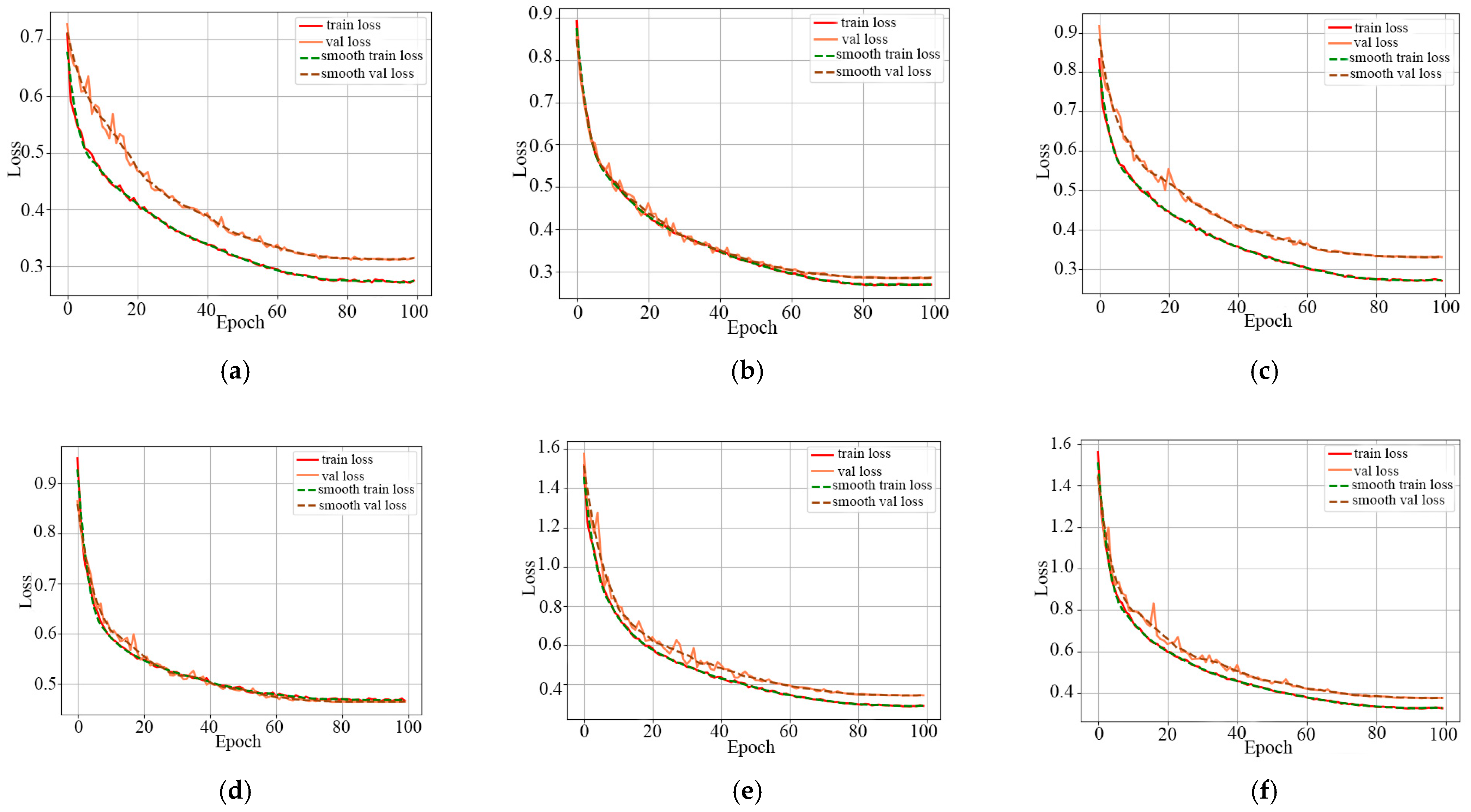
Figure 5 displays the training loss curves of six models on the PCA dataset, all showing a downward trend and gradually stabilising. Most models exhibited rapid loss reduction within the first 50 epochs, followed by a gradual convergence phase. Some models ultimately stabilised with losses below 0.3, while a few remained slightly above 0.3. All training was conducted under identical configurations, with the curve variations reflecting the fundamental convergence behaviour of each method on this dataset.

3.4. Accuracy Evaluation Method

This study selected five indicators to evaluate the results of the semantic segmentation models, including intersection-over-union (IoU), mean intersection-over-union (mIoU), pixel accuracy (PA), F1 index (F1-score), and overall accuracy (OA). These evaluation metrics can be calculated using a confusion matrix, as shown in Table 2. Among these, IoU, PA, and F1-score were used to evaluate the separability between wheat and corn, while mIoU, OA, and average F1-score were used to evaluate the overall classification results.
The intersection-over-union (IoU) is the ratio of the intersection between the true values and predicted values of a certain category calculated by the model to the union of the two sets [44]. The closer the value is to 1, the closer the predicted results are to the actual values. The formula is as follows:
IOU = X Y X Y = TP TP + FN + FP
The mean intersection-over-union (mIoU) is calculated by summing the intersection-over-union (IoU) values for each category computed by the model and then taking the average. The formula is as follows:
m IoU = 1 k + 1 i = 0 κ TP i TP i + FN i + FP i
Pixel accuracy (PA) expresses the proportion of pixels in an image that are correctly classified out of the total number of pixels in the image. The formula for calculating PA is as follows:
P A = TP + TN TP + FP + FN + TN
m PA = 1 k + 1 i = 0 κ TP i TP i + FP i
The F1-score is the harmonic mean calculated using the accuracy and recall rates of a certain category in the classification results. Precision refers to the proportion of positive examples that are predicted to be positive by the model and are indeed positive examples out of all positive examples. Recall refers to the proportion of all positive samples that are correctly predicted. The formulas for calculating precision, recall, and F1 score [45] are as follows:
Precision = TP TP + FP
Recall = TP TP + FN
F 1 = 2 Precision Recall Precision + Recall
Overall accuracy refers to the ratio of the number of pixels correctly predicted by the model to the total number of pixels, and can be used as one of the evaluation indicators for the overall accuracy of the model. The calculation formula [46] is as follows:
O A = TP + TN TP + FN + FP + TN

4. Results and Analysis

4.1. Time-Series Characteristics of Vegetation Indices for Wheat and Corn

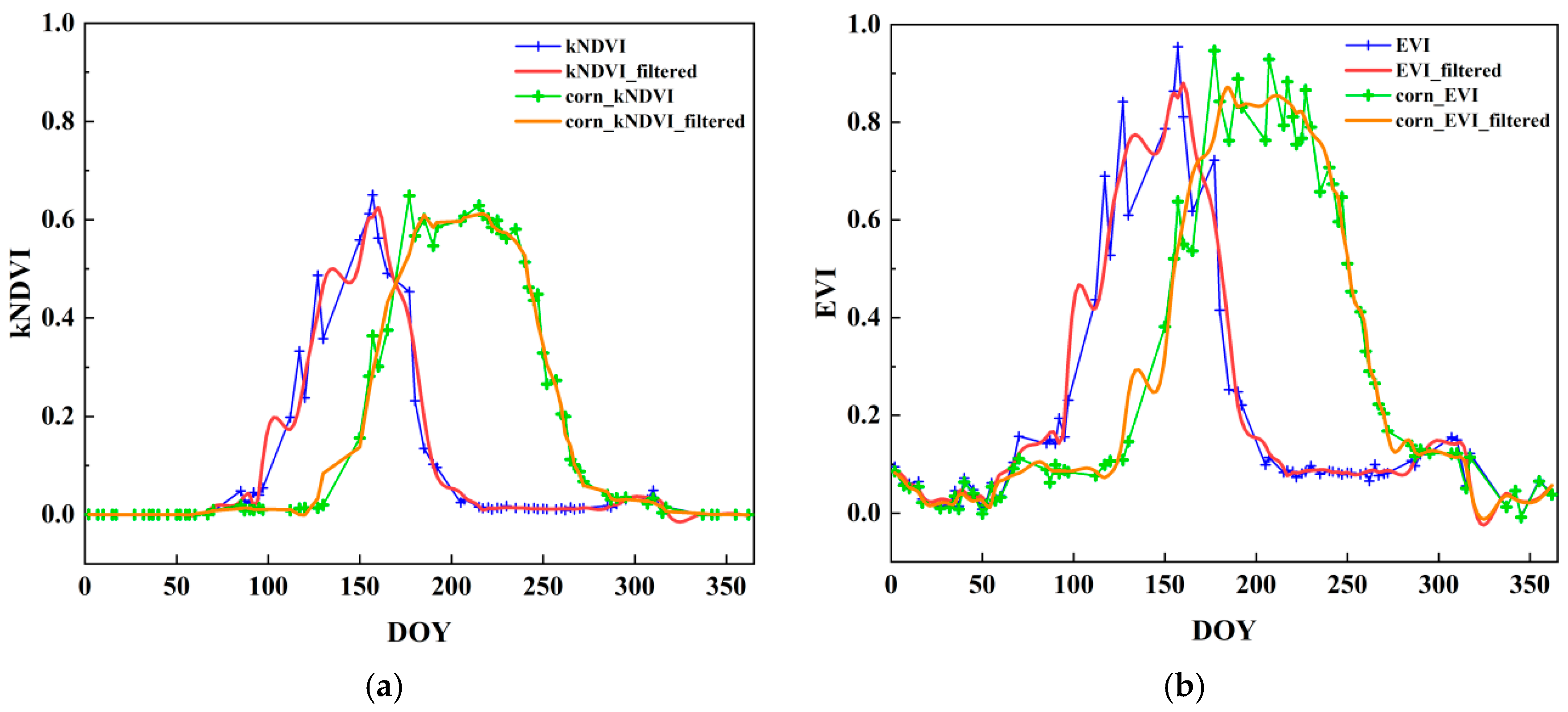
This study utilised the GEE platform and Sentinel-2 satellite time-series data to calculate vegetation indices for wheat and corn in the study area and plotted time-series characteristic curves (Figure 6). The findings indicated that S-G filtering led to a notable reduction in noise within the kNDVI and EVI curves. For wheat and corn, the kNDVI and EVI curves—both before and after filtering—exhibited analogous overall trends and consistent variations. Additionally, the kNDVI values of these two crops were consistently lower than their corresponding EVI values, and the fluctuations in kNDVI were also significantly less pronounced than those in EVI.
Figure 6 shows the annual phenological characteristics of wheat and corn. The figure shows that the vegetation index trends of the two are similar, but there were obvious differences in terms of timing. Wheat sowing began around the 90th day, the kNDVI and EVI began to rise significantly, reaching a peak around the 150th day after sowing and then gradually declining. In comparison, corn was usually planted around 100 days after sowing, and the kNDVI and EVI peaked around 200 days after sowing and then began to decline.

4.2. Comparison and Analysis of Experimental Results from Different Datasets

In order to verify the semantic segmentation performance of the different semantic segmentation models on wheat and corn, as well as the impact of optical remote sensing images after PCA on segmentation capabilities. This study selected five semantic segmentation models, namely DeeplabV3+, PSPnet, HRnet, Segformer, and U-Net, for comparison and evaluated the segmentation capabilities of our newly improved model. The main results are shown in Table 3 and Table 4 below.
Table 3 and Table 4 show the crop extraction accuracy results achieved by the different semantic segmentation models on true colour datasets and principal component transformation datasets. In the RGB dataset, the mIoU, mPA, F1-score, and OA metrics of the proposed model were 81.31%, 90.19%, 89.67%, and 90.07%, respectively. Compared with the DeepLabv3+, PSPnet, HRnet, Segformer, and U-Net methods, the OA improved by 5.82%, 4.44%, 2.13%, 10.16%, and 2.46%, respectively, using our proposed model. In the dataset after PCA transformation, the proposed model achieved mIoU, mPA, F1-score, and OA scores of 83.03%, 91.34%, 90.73%, and 90.91%, respectively. Compared with DeepLabv3+, PSPnet, HRnet, Segformer, and U-Net methods, the proposed method achieves an OA improvement of 5.97%, 4.55%, 2.03%, 8.99%, and 1.5%, respectively. Compared with the true colour dataset, DeepLabv3+, PSPnet, HRnet, Segformer, U-Net, and the improved U-Net model performed better in extracting features from the PCA dataset, with OA improvements of 0.69%, 0.73%, 0.94%, 2.01%, 1.80%, and 0.84%, respectively. The results showed that the model we proposed performs better in extracting wheat and corn from the dataset after principal component transformation.

4.3. Comparison of Mapping Results from Different Algorithms

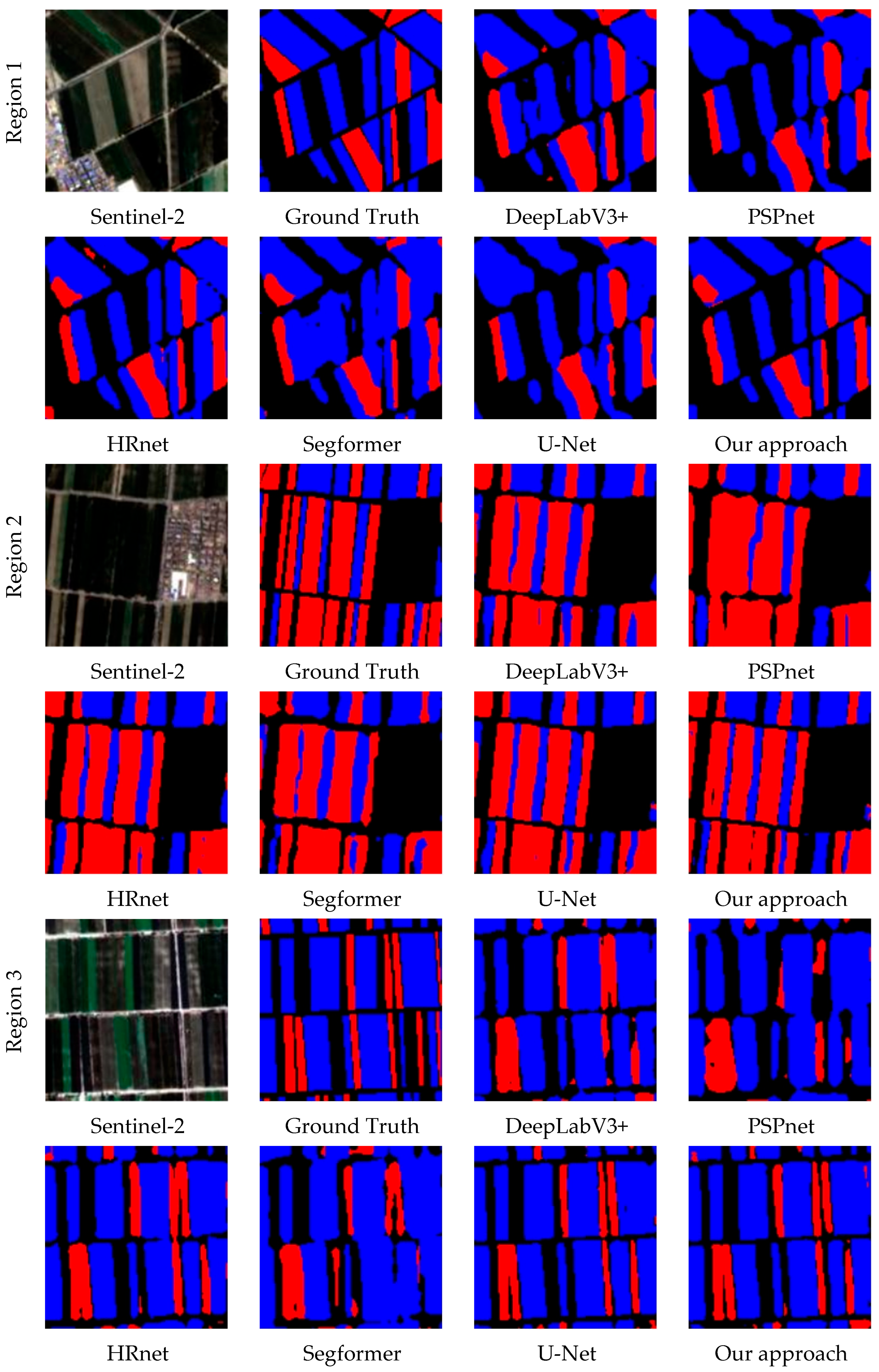
Figure 7 presents the prediction results of each model under the different scenarios. Specifically, Region 1 demonstrates the models’ prediction results in complex scenarios; Region 2 demonstrates their results in areas dominated by wheat; and Region 3 illustrates their results in areas where corn is the primary crop.
As can be seen from Figure 7, the improved U-Net model can effectively identify winter wheat and corn, clearly distinguishing between the two crops regardless of whether they were grown on large or small farmland areas. In particular, the improved U-Net model outperformed the other models in terms of edge detail recognition and was highly consistent with the actual ground data. The recognition results of the HRnet, Segformer, PSPnet, and DeeplabV3+ models were rather confusing, with fragmented misclassifications appearing in certain areas of the predicted images. The identification results of these models showed blurred farmland boundaries, especially PSPnet, where some farmland contours were unclear. The U-Net model had poor detail recognition capabilities and failed to recognise some small farmlands and ignored some edge detail information. Overall, the models showed varying degrees of effectiveness in identifying wheat and corn, but the improved U-Net model performed the best.

4.4. Ablation Experiment

We set up ablation experiments based on the U-Net model to test the impact of the improved model on semantic segmentation networks.
Experiment 1: Set the U-Net model with ResNet50 as the backbone network as the baseline model.
Experiment 2: Add the CBAM to the upsampling layer and downsampling layer based on Experiment 1.
Experiment 3: Add the improved ASPP model to the end of the backbone network based on the model structure of Experiment 1;
Experiment 4: Add the CBAM model and the improved ASPP module separately based on Experiment 1.
The experimental results are shown in Table 5.
As shown in the table, the mIoU and F1-score of the original U-Net network were 80.43% and 89.14%, respectively. After adding the CBAM to the encoder and decoder, the mIoU and F1-score improved by 2.40% and 1.47%, respectively, showing a significant improvement compared to the baseline model. After adding the improved ASPP module to the baseline model, the mIoU and F1-score improved by 1.28% and 0.79%, respectively. The experimental results showed that replacing the backbone network in the original U-Net network and adding the CBAM attention mechanism and the improved ASPP module can effectively improve the segmentation performance of the model, fully proving that the above model improvements are effective.

4.5. Model Generality Analysis

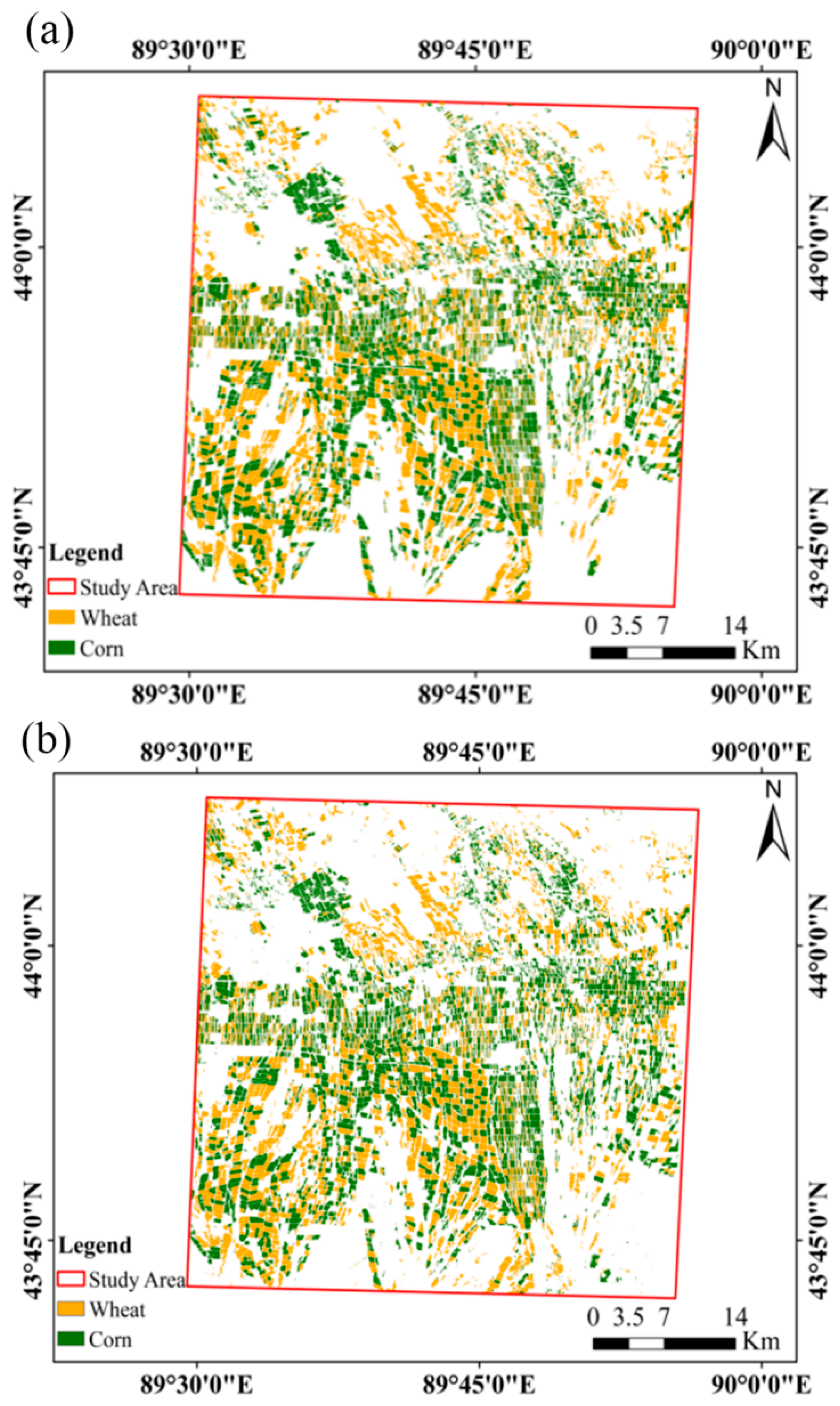
In order to further verify the generalisability of the method proposed in this study, it was applied to the spatial distribution prediction of wheat and corn in Qitai County, and the corresponding spatial distribution maps were drawn (Figure 8).
The testing accuracy is shown in Figure 9. The extraction accuracy for wheat and corn in Qitai County was comparable to the results from the research area. The OA, mIoU, mPA, and F1-score of the predicted results were 89.98%, 81.32%, 90.55%, and 89.69%, respectively. Compared with the results from the study area, the errors of all the evaluation indicators were less than 2%. Overall, the extracted wheat and corn results were close to the actual situation, indicating that the model had good generalisation capabilities and great potential for further promotion and application.

5. Discussion

5.1. The Impact of Principal Component Analysis on the Results

The results showed that the modelling accuracy using the dataset obtained based on PCA in this study was higher than that using the RGB dataset. Zhang et al. [12] achieved an F1-score of 84.59% for wheat recognition using RGB data. Narvaria et al. [47] achieved an OA of 83.85% for crop recognition using RGB data. Zhang et al. [48] obtained an OA of 79.58% for crop recognition (including corn) using RGB data. The modelling accuracy based on RGB in this study was higher compared with the evaluation indicators in previous studies. This indicated that the RGB dataset constructed in this study has a certain degree of reliability in identifying wheat and corn. However, although RGB datasets can easily achieve high spatial and temporal resolution, it only contains visible light bands (red, green, and blue) and lacks other spectral information, which reduces the ability to distinguish crop type pixels in different environments [49]. To this end, this study also introduced a PCA dataset to enhance the separability of spectrally similar crops such as wheat and corn.
Compared with the RGB dataset, the average accuracy for detecting corn and wheat in this study improved by 1.16% with the support of existing algorithms and PCA datasets. Using the PCA dataset, each model—including DeepLabv3+, PSPnet, HRnet, Segformer, U-Net, and the improved U-Net—achieved OA improvements of 0.69%, 0.73%, 0.94%, 2.01%, 1.80%, and 0.84% in sequence. These results indicate that the PCA dataset provides certain benefits for multiple models. Compared with existing algorithms, the new algorithm developed in this study showed an average accuracy improvement of 1.19% with the support of the PCA dataset, demonstrating the synergistic advantages of the improved model and PCA data.
In this study, PCA played an important role in improving the accuracy of wheat and corn identification. By reconstructing the dataset, PCA effectively reduced the data redundancy and noise interference while preserving key spectral information [50]. In comparison to the RGB dataset, the PCA dataset incorporated spectral information (e.g., visible light and near-infrared light), which significantly enhanced the model’s capability to distinguish between wheat and corn. In summary, the study concluded that the dataset generated based on PCA can serve as an important supplement to the RGB dataset.

5.2. Time Window for Vegetation Index

By analysing the kNDVI and EVI time series curves, this study found that the period from day 156 to day 176 was the optimal window for identifying wheat and corn. By leveraging vegetation index time series, crop phenological information can be effectively captured; this approach has been widely adopted for crop classification purposes. Under certain conditions, EVI time series can better described crop phenological information than NDVI time series. Yet, in handling saturation effects and seasonal variations, the kNDVI outperformed the NDVI.
From the time series curves (Figure 6), wheat entered the heading to maturity stage between days 156 and 176, showing high kNDVI and EVI values. Corn, on the other hand, was in the seedling stage during this period, with vegetation index values significantly lower than those of wheat, resulting in a significant difference between the two [51,52]. This phenological off-peak period provided a critical time window for identifying the two types of crops.
It is worth noting that the optimal identification window period still needs to be further adjusted in combination with climate, meteorological and other factors [52]. For example, in years with warm winters or rapid warming in spring, wheat greening and jointing may occur earlier, which may cause changes in the time series curve and affect the optimal identification time. Therefore, subsequent research should integrate multi-year time series data to develop a dynamic window prediction model that relies on climatic factors.

5.3. Algorithm Performance

The research results indicated that the improved U-Net model proposed in this study demonstrated superior modelling accuracy compared to traditional semantic segmentation models for wheat and corn recognition, both on the RGB dataset and the PCA dataset. In previous studies, Zhao et al. [53] proposed the U-Net-CBMA model, which achieved an mIoU of 77.1% in similar tasks; Li et al. [54] used the U-Net model to achieve an mIoU of 75.13% in crop recognition in the Hetao Irrigation District; and Zhang et al. [55] employed the U-Net model, achieving a mean intersection-over-union (mIoU) of 76.01% for wheat recognition. In our study, the proposed model achieved an mIoU of 83.13% in the wheat and corn identification task, representing improvements of 6.02%, 8%, and 7.12% compared to previous studies and thus demonstrating its capability to identify wheat and corn in complex environments.
The experimental results (see Table 3 and Table 4) demonstrated that the recognition accuracy of our model improved to varying extents across the different datasets. On the RGB dataset, our model achieved overall accuracy (OA) improvements of 5.82%, 4.44%, 2.13%, 10.16%, and 2.46% compared to DeepLabV3+, PSPnet, HRnet, Segformer, and the standard U-Net, respectively. On the PCA dataset, the proposed model attained OA improvements of 5.97%, 4.55%, 2.03%, 8.99%, and 1.5% relative to the aforementioned baseline models. These improvements not only confirmed the effectiveness of our model modifications but also underscored the influence of different datasets on semantic segmentation performance.
The improvement in the performance of this research model was mainly due to several targeted optimisations of the network structure. First, this study introduced the CBAM attention mechanism into the deep layers of the encoder. This attention mechanism allows the model to focus more on information in key areas and ignore irrelevant information [37]. As shown in the experimental results (Table 5), the mIoU and F1-score of the U-Net model with the CBAM attention mechanism improved by 2.40% and 1.47%, respectively, compared to the traditional U-Net model. Therefore, the introduction of the CBAM attention mechanism effectively improved the performance of the U-Net model, enabling the model to focus more on key areas and effectively alleviating the problem of wheat and corn confusion. Secondly, the model included an ASPP module, which captures objects and contextual information at different scales by utilising multi-expansion rate spatial convolution [42]. As shown in the experimental results (Table 5), adding the improved ASPP module to the U-Net model improved the mIoU and F1-score by 1.28% and 0.79%, respectively. This design effectively addressed issues such as uneven field sizes and fragmented boundaries, enhancing the ability to identify small-area farmland and complex planting patterns.
To further improve the efficiency of the model, this study maximised the reduction in computational costs by replacing traditional standard convolutions with separable convolutions in the ASPP module [43]. This method can effectively reduce the model’s memory usage and training time (Table 6). In addition, CBAM is a lightweight attention mechanism module that can be easily embedded into the model without any additional computation [56], enhancing model performance while reducing computational complexity.
It is worth noting that although this study conducted generalisation testing in Qitai County, both the test area and training area are located within the Xinjiang region and share highly similar crop structures, climatic conditions, and other parameters. Consequently, the model’s transferability to other regions remains unverified. Moving forward, we will endeavour to construct training datasets spanning multiple regions and years, thereby expanding the spatio-temporal coverage of the dataset.

5.4. Extraction Efficiency of Crop Types

The results of this study indicated that the extraction results for wheat and corn in the study area were clear-cut, spatially accurate, and precisely categorised. In previous studies, Zhang et al. [37] reached an OA of 87.89% for winter wheat identification, while Diao et al. [57] obtained an mPA of 90.18% for corn identification. However, the method proposed herein attained an OA of 90.91% and an mPA of 91.34% for wheat and corn identification, respectively. This slight accuracy improvement over previous methods demonstrates the reliability of the proposed method for segmenting wheat and corn.
This study demonstrated the ability of the proposed method to distinguish between wheat and corn in terms of both quantitative accuracy and spatial distribution. As can be seen from the experimental results (Table 4), the IoU and PA for wheat identification were 82.37% and 92.07%, respectively; the IoU and PA for corn identification were 82.16% and 92.68%, respectively. The identification accuracy for both types of crops was at a high level and the indicators were similar, indicating that the method proposed in this study can maintain a stable discrimination ability when dealing with crops with similar spectral characteristics. From the local results (Figure 7), the boundaries of the main planting areas were clear, and there were few misclassified areas. The overall classification results showed a high degree of field matching, with no obvious fragmentation or abnormal patches. From the overall results (Figure 8), the crop distribution was highly consistent with the actual situation. In particular, the classification results in contiguous planting areas were consistent with the actual situation.
The improvement in segmentation accuracy was the result of multiple factors working together. The time series curves effectively captured the phenological differences between wheat and corn during their growing seasons and determined the optimal window period for distinguishing between wheat and corn. The PCA dataset retained the main spectral information of remote sensing images while reducing data redundancy [50], making it easier for the model to distinguish between different crops. The improved U-Net model introduces the CBAM attention mechanism and an improved ASPP module, further enhancing the model’s recognition capabilities in complex environments.

6. Conclusions

This study combined phenological information on wheat and corn and analysed their kNDVI and EVI time-series vegetation indices to determine the optimal extraction time range. An improved U-Net model was used to extract spatial distribution information on wheat and corn in the study area. The specific conclusions were as follows.
The phenological characteristics of wheat and corn differ significantly within the study area. This study determined the optimal time for identifying wheat and corn by examining the time series of the vegetation indices for wheat and corn. The results indicated that the wheat and corn in the study area were in the growth and development stage between 156 and 176 days and exhibited distinct characteristics, making this the optimal time for identifying wheat and corn.
This study proposed a lightweight model for extracting wheat and corn based on the U-Net semantic segmentation model, combined with an CBAM attention mechanism module and an improved ASPP module. Based on this model, the extraction results for wheat and corn in the study area achieved an mIoU of 83.03%, mPA of 91.34%, F1-score of 90.73%, and overall accuracy of 90.91%, all of which were superior to the comparison model. At the same time, the model’s versatility was also validated in other areas. Overall, this model reduces the number of parameters and training time while ensuring model extraction accuracy. It had strong generalisation capabilities and is worthy of further promotion and application.
This study constructed a dataset using PCA, abandoning the traditional RGB true colour dataset, effectively solving the problem of poor extraction results caused by insufficient information in the model. The results showed that the dataset after PCA can effectively reduce the impact of spectral differences. This dataset can help suppress noise interference in remote sensing images. Compared with other semantic segmentation models, the model used in this study achieved an average mIoU improvement of approximately 2.43%.

Author Contributions

Conceptualization, F.W. and Y.W.; methodology, Y.W.; software, X.G.; validation, H.H., X.L. and X.G.; formal analysis, F.W. and Y.L.; investigation, X.G. and R.L.; resources, F.W. and Y.L.; data curation, X.G. and H.H.; writing—original draft preparation, Y.W. and Y.L.; writing—review and editing, F.W.; funding acquisition, F.W. All authors have read and agreed to the published version of the manuscript.

Funding

This study was supported by the National Natural Science Foundation of China (42101363). This project was also supported by the Research Initiation Fund of Chengdu University (2081923044 and 2081923045).

Data Availability Statement

The original contributions presented in the study are included in the article; further inquiries can be directed to the corresponding author.

Conflicts of Interest

The authors declare no conflicts of interest.

References

  1. Sishodia, R.; Ray, R.; Singh, S. Applications of Remote Sensing in Precision Agriculture: A Review. Remote Sens. 2020, 12, 3136. [Google Scholar] [CrossRef]
  2. Weiss, M.; Jacob, F.; Duveiller, G. Remote Sensing for Agricultural Applications: A Meta-Review. Remote Sens. Environ. 2020, 236, 111402. [Google Scholar] [CrossRef]
  3. Qiu, B.; Lu, D.; Tang, Z.; Song, D.; Zeng, Y.; Wang, Z.; Chen, C.; Chen, N.; Huang, H.; Xu, W. Mapping Cropping Intensity Trends in China during 1982–2013. Appl. Geogr. 2017, 79, 212–222. [Google Scholar] [CrossRef]
  4. You, N.; Dong, J.; Huang, J.; Du, G.; Zhang, G.; He, Y.; Yang, T.; Di, Y.; Xiao, X. The 10-m Crop Type Maps in Northeast China during 2017–2019. Sci. Data 2021, 8, 41. [Google Scholar] [CrossRef]
  5. Massey, R.; Sankey, T.; Congalton, R.; Yadav, K.; Thenkabail, P.; Ozdogan, M.; Meador, A. MODIS Phenology-Derived, Multi-Year Distribution of Conterminous US Crop Types. Remote Sens. Environ. 2017, 198, 490–503. [Google Scholar] [CrossRef]
  6. Cheng, Z.; Gu, X.; Zhou, Z.; Yin, R.; Zheng, X.; Li, W.; Cai, W.; Chang, T.; Du, Y. Crop Aboveground Biomass Monitoring Model Based on UAV Spectral Index Reconstruction and Bayesian Model Averaging: A Case Study of Film-Mulched Wheat and Maize. Comput. Electron. Agric. 2024, 224, 109190. [Google Scholar] [CrossRef]
  7. Lu, B.; Dao, P.; Liu, J.; He, Y.; Shang, J. Recent Advances of Hyperspectral Imaging Technology and Applications in Agriculture. Remote Sens. 2020, 12, 2659. [Google Scholar] [CrossRef]
  8. Farrell, M.; Macdonald, L.; Butler, G.; Chirino-Valle, I.; Condron, L. Biochar and Fertiliser Applications Influence Phosphorus Fractionation and Wheat Yield. Biol. Fertil. Soils 2014, 50, 169–178. [Google Scholar] [CrossRef]
  9. Ding, L.; Zhang, J.; Bruzzone, L. Semantic Segmentation of Large-Size VHR Remote Sensing Images Using a Two-Stage Multiscale Training Architecture. IEEE Trans. Geosci. Remote Sens. 2020, 58, 5367–5376. [Google Scholar] [CrossRef]
  10. Zhao, L.; Wang, C.; Wang, T.; Liu, J.; Qiao, Q.; Yang, Y.; Hu, P.; Zhang, L.; Zhao, S.; Chen, D.; et al. Identification of the Candidate Gene Controlling Tiller Angle in Common Wheat through Genome-Wide Association Study and Linkage Analysis. Crop J. 2023, 11, 870–877. [Google Scholar] [CrossRef]
  11. Zhou, K.; Zhang, Z.; Liu, L.; Miao, R.; Yang, Y.; Ren, T.; Yue, M. Research on SU-Net Winter Wheat Identification Method Based on GF-2. Remote Sens. 2023, 15, 3094. [Google Scholar] [CrossRef]
  12. Zhang, Q.; Wang, G.; Wang, G.; Song, W.; Wei, X.; Hu, Y. Identifying Winter Wheat Using Landsat Data Based on Deep Learning Algorithms in the North China Plain. Remote Sens. 2023, 15, 5121. [Google Scholar] [CrossRef]
  13. Zhao, G.; Chang, X.; Wang, D.; Tao, Z.; Wang, Y.; Yang, Y.; Zhu, Y. General Situation and Development of Wheat Production. Crops 2018, 4, 1–7. [Google Scholar]
  14. He, Q.; Zhou, G. The Climatic Suitability for Maize Cultivation in China. Chin. Sci. Bull. 2012, 57, 395–403. [Google Scholar] [CrossRef]
  15. Immitzer, M.; Vuolo, F.; Atzberger, C. First Experience with Sentinel-2 Data for Crop and Tree Species Classifications in Central Europe. Remote Sens. 2016, 8, 166. [Google Scholar] [CrossRef]
  16. Qi, H.; Qian, X.; Shang, S.; Wan, H. Multi-Year Mapping of Cropping Systems in Regions with Smallholder Farms from Sentinel-2 Images in Google Earth Engine. Giscience Remote Sens. 2024, 61, 2309843. [Google Scholar] [CrossRef]
  17. Wei, P.; Ye, H.; Qiao, S.; Liu, R.; Nie, C.; Zhang, B.; Song, L.; Huang, S. Early Crop Mapping Based on Sentinel-2 Time-Series Data and the Random Forest Algorithm. Remote Sens. 2023, 15, 3212. [Google Scholar] [CrossRef]
  18. Hao, P.; Zhan, Y.; Wang, L.; Niu, Z.; Shakir, M. Feature Selection of Time Series MODIS Data for Early Crop Classification Using Random Forest: A Case Study in Kansas, USA. Remote Sens. 2015, 7, 5347–5369. [Google Scholar] [CrossRef]
  19. Yu, L.; Tao, H.; Li, Q.; Xie, H.; Xu, Y.; Mahemujiang, A.; Jiang, Y. Research on Machine Learning-Based Extraction and Classification of Crop Planting Information in Arid Irrigated Areas Using Sentinel-1 and Sentinel-2 Time-Series Data. Agriculture 2025, 15, 1196. [Google Scholar] [CrossRef]
  20. Sheykhmousa, M.; Mahdianpari, M.; Ghanbari, H.; Mohammadimanesh, F.; Ghamisi, P.; Homayouni, S. Support Vector Machine Versus Random Forest for Remote Sensing Image Classification: A Meta-Analysis and Systematic Review. IEEE J. Sel. Top. Appl. Earth Obs. Remote Sens. 2020, 13, 6308–6325. [Google Scholar] [CrossRef]
  21. Wang, Y.; Gu, L.; Jiang, T.; Gao, F. MDE-U-Net: A Multitask Deformable U-Net Combined Enhancement Network for Farmland Boundary Segmentation. IEEE Geosci. Remote Sens. Lett. 2023, 20, 1–5. [Google Scholar] [CrossRef]
  22. Zhang, M.; Su, W.; Fu, Y.; Zhu, D.; Xue, J.; Huang, J.; Wang, W.; Wu, J.; Yao, C. Super-Resolution Enhancement of Sentinel-2 Image for Retrieving LAI and Chlorophyll Content of Summer Corn. Eur. J. Agron. 2019, 111, 125938. [Google Scholar] [CrossRef]
  23. Dong, J.; Xiao, X.; Menarguez, M.; Zhang, G.; Qin, Y.; Thau, D.; Biradar, C.; Moore, B. Mapping Paddy Rice Planting Area in Northeastern Asia with Landsat 8 Images, Phenology-Based Algorithm and Google Earth Engine. Remote Sens. Environ. 2016, 185, 142–154. [Google Scholar] [CrossRef] [PubMed]
  24. Alam, F.; Zhou, J.; Liew, A.; Jia, X.; Chanussot, J.; Gao, Y. Conditional Random Field and Deep Feature Learning for Hyperspectral Image Classification. IEEE Trans. Geosci. Remote Sens. 2019, 57, 1612–1628. [Google Scholar] [CrossRef]
  25. Li, Y.; Liu, W.; Ge, Y.; Yuan, S.; Zhang, T.; Liu, X. Extracting Citrus-Growing Regions by Multiscale U-Net Using Sentinel-2 Satellite Imagery. Remote Sens. 2024, 16, 36. [Google Scholar] [CrossRef]
  26. Chang, Z.; Li, H.; Chen, D.; Liu, Y.; Zou, C.; Chen, J.; Han, W.; Liu, S.; Zhang, N. Crop Type Identification Using High-Resolution Remote Sensing Images Based on an Improved DeepLabV3+ Network. Remote Sens. 2023, 15, 5088. [Google Scholar] [CrossRef]
  27. Bian, Y.; Li, L.; Jing, W. CACPU-Net: Channel Attention U-Net Constrained by Point Features for Crop Type Mapping. Front. Plant Sci. 2023, 13, 1030595. [Google Scholar] [CrossRef]
  28. Zhang, Z.; Zhang, H.; Xu, E. Enhancing the Digital Mapping Accuracy of Farmland Soil Organic Carbon in Arid Areas Using Agricultural Land Use History. J. Clean. Prod. 2022, 334, 130232. [Google Scholar] [CrossRef]
  29. Peng, Y.; Liu, W.; Xiong, C.; Bai, X. Value Transformation and Ecological Practice: The Path to Realizing the Value of Ecotourism Products in Heritage Sites-A Case Study of the Qitai Dry Farming System in Xinjiang. Sustainability 2024, 16, 5031. [Google Scholar] [CrossRef]
  30. Malinowski, R.; Lewinski, S.; Rybicki, M.; Gromny, E.; Jenerowicz, M.; Krupinski, M.; Nowakowski, A.; Wojtkowski, C.; Krupinski, M.; Krätzschmar, E.; et al. Automated Production of a Land Cover/Use Map of Europe Based on Sentinel-2 Imagery. Remote Sens. 2020, 12, 3523. [Google Scholar] [CrossRef]
  31. Gao, H.; Li, R.; Shen, Q.; Yao, Y.; Shao, Y.; Zhou, Y.; Li, W.; Li, J.; Zhang, Y.; Liu, M. Deep-Learning-Based Automatic Extraction of Aquatic Vegetation from Sentinel-2 Images-A Case Study of Lake Honghu. Remote Sens. 2024, 16, 867. [Google Scholar] [CrossRef]
  32. Camps-Valls, G.; Campos-Taberner, M.; Moreno-Martínez, A.; Walther, S.; Duveiller, G.; Cescatti, A.; Mahecha, M.; Muñoz-Marí, J.; García-Haro, F.; Guanter, L.; et al. A Unified Vegetation Index for Quantifying the Terrestrial Biosphere. Sci. Adv. 2021, 7, eabc7447. [Google Scholar] [CrossRef] [PubMed]
  33. Feng, X.; Tian, J.; Wang, Y.; Wu, J.; Liu, J.; Ya, Q.; Li, Z. Spatio-Temporal Variation and Climatic Driving Factors of Vegetation Coverage in the Yellow River Basin from 2001 to 2020 Based on kNDVI. Forests 2023, 14, 620. [Google Scholar] [CrossRef]
  34. Gu, Z.; Chen, X.; Ruan, W.; Zheng, M.; Gen, K.; Li, X.; Deng, H.; Chen, Y.; Liu, M. Quantifying the Direct and Indirect Effects of Terrain, Climate and Human Activity on the Spatial Pattern of kNDVI-Based Vegetation Growth: A Case Study from the Minjiang River Basin, Southeast China. Ecol. Inform. 2024, 80, 102493. [Google Scholar] [CrossRef]
  35. Ronneberger, O.; Fischer, P.; Brox, T. U-Net: Convolutional Networks for Biomedical Image Segmentation. In Medical Image Computing and Computer-Assisted Intervention—MICCAI 2015; Navab, N., Hornegger, J., Wells, W., Frangi, A., Eds.; Springer: Cham, Switzerland, 2015; Volume 9351, pp. 234–241. [Google Scholar]
  36. Li, J.; Mao, J.; Chen, C.; Bi, Z. Research on the Remote Sensing Change Detection of Land Cover Types in Agricultural-Forestry Transition Zone Based on CNN-Transformer Hybrid Model. In Proceedings of the 2025 6th International Conference on Computer Vision, Image and Deep Learning (CVIDL), Ningbo, China, 23–25 May 2025; IEEE: New York, NY, USA; pp. 546–551. [Google Scholar]
  37. Zhang, Y.; Wang, H.; Liu, J.; Zhao, X.; Lu, Y.; Qu, T.; Tian, H.; Su, J.; Luo, D.; Yang, Y. A Lightweight Winter Wheat Planting Area Extraction Model Based on Improved DeepLabv3+ and CBAM. Remote Sens. 2023, 15, 4156. [Google Scholar] [CrossRef]
  38. Liu, J.; Zhang, Y.; Liu, C.; Liu, X. Monitoring Impervious Surface Area Dynamics in Urban Areas Using Sentinel-2 Data and Improved Deeplabv3+ Model: A Case Study of Jinan City, China. Remote Sens. 2023, 15, 1976. [Google Scholar] [CrossRef]
  39. Yang, X.; Fan, X.; Peng, M.; Guan, Q.; Tang, L. Semantic Segmentation for Remote Sensing Images Based on an AD-HRNet Model. Int. J. Digit. Earth 2022, 15, 2376–2399. [Google Scholar] [CrossRef]
  40. Wang, C.; Zhang, R.; Chang, L. A Study on the Dynamic Effects and Ecological Stress of Eco-Environment in the Headwaters of the Yangtze River Based on Improved DeepLab V3+ Network. Remote Sens. 2022, 14, 2225. [Google Scholar] [CrossRef]
  41. Chollet, F. Xception: Deep Learning with Depthwise Separable Convolutions. In Proceedings of the 2017 IEEE Conference on Computer Vision and Pattern Recognition (CVPR), Honolulu, HI, USA, 21–26 July 2017; IEEE: New York, NY, USA; pp. 1800–1807. [Google Scholar]
  42. Chen, L.; Papandreou, G.; Kokkinos, I.; Murphy, K.; Yuille, A. DeepLab: Semantic Image Segmentation with Deep Convolutional Nets, Atrous Convolution, and Fully Connected CRFs. IEEE Trans. Pattern Anal. Mach. Intell. 2018, 40, 834–848. [Google Scholar] [CrossRef]
  43. Shin, S.; Lee, S.; Han, H. EAR-Net: Efficient Atrous Residual Network for Semantic Segmentation of Street Scenes Based on Deep Learning. Appl. Sci. 2021, 11, 9119. [Google Scholar] [CrossRef]
  44. Yang, B.; Zhu, Y.; Zhou, S. Accurate Wheat Lodging Extraction from Multi-Channel UAV Images Using a Lightweight Network Model. Sensors 2021, 21, 6826. [Google Scholar] [CrossRef]
  45. Diakogiannis, F.; Waldner, F.; Caccetta, P.; Wu, C. ResU-Net-a: A Deep Learning Framework for Semantic Segmentation of Remotely Sensed Data. ISPRS J. Photogramm. Remote Sens. 2020, 162, 94–114. [Google Scholar] [CrossRef]
  46. Tang, Z.; Sun, Y.; Wan, G.; Zhang, K.; Shi, H.; Zhao, Y.; Chen, S.; Zhang, X. Winter Wheat Lodging Area Extraction Using Deep Learning with GaoFen-2 Satellite Imagery. Remote Sens. 2022, 14, 4887. [Google Scholar] [CrossRef]
  47. Narvaria, A.; Kumar, U.; Jhanwwee, K.S.; Dasgupta, A.; Kaur, G.J. Classification and Identification of Crops Using Deep Learning with UAV Data. In Proceedings of the 2021 IEEE International India Geoscience and Remote Sensing Symposium (InGARSS), Ahmedabad, India, 6–10 December 2021; IEEE: New York, NY, USA; pp. 153–156. [Google Scholar]
  48. Zhang, J.; Zhao, L.; Yang, H. A Dual-Branch U-Net for Staple Crop Classification in Complex Scenes. Remote Sens. 2025, 17, 726. [Google Scholar] [CrossRef]
  49. Mei, S.; Geng, Y.; Hou, J.; Du, Q. Learning Hyperspectral Images from RGB Images via a Coarse-to-Fine CNN. Sci. China Inf. Sci. 2022, 65, 152102. [Google Scholar] [CrossRef]
  50. Diao, Z.; Guo, P.; Zhang, B.; Yan, J.; He, Z.; Zhao, S.; Zhao, C.; Zhang, J. Spatial-Spectral Attention-Enhanced Res-3D-OctConv for Corn and Weed Identification Utilizing Hyperspectral Imaging and Deep Learning. Comput. Electron. Agric. 2023, 212, 108092. [Google Scholar] [CrossRef]
  51. Han, D.; Wang, P.; Li, Y.; Zhang, Y.; Guo, J. Mapping the Main Phenological Spatiotemporal Changes of Summer Maize in the Huang-Huai-Hai Region Based on Multiple Remote Sensing Indices. Agronomy 2025, 15, 1182. [Google Scholar] [CrossRef]
  52. Yue, J.; Li, T.; Shen, J.; Wei, Y.; Xu, X.; Liu, Y.; Feng, H.; Ma, X.; Li, C.; Yang, G.; et al. Winter Wheat Maturity Prediction via Sentinel-2 MSI Images. Agriculture 2024, 14, 1368. [Google Scholar] [CrossRef]
  53. Zhao, J.; Wang, J.; Qian, H.; Zhan, Y.; Lei, Y. Extraction of Winter-Wheat Planting Areas Using a Combination of U-Net and CBAM. Agronomy 2022, 12, 2965. [Google Scholar] [CrossRef]
  54. Li, G.; Han, W.; Dong, Y.; Zhai, X.; Huang, S.; Ma, W.; Cui, X.; Wang, Y. Multi-Year Crop Type Mapping Using Sentinel-2 Imagery and Deep Semantic Segmentation Algorithm in the Hetao Irrigation District in China. Remote Sens. 2023, 15, 875. [Google Scholar] [CrossRef]
  55. Zhang, M.; Xue, Y.; Zhan, Y.; Zhao, J. Semi-Supervised Semantic Segmentation-Based Remote Sensing Identification Method for Winter Wheat Planting Area Extraction. Agronomy 2023, 13, 2868. [Google Scholar] [CrossRef]
  56. Ma, R.; Wang, J.; Zhao, W.; Guo, H.; Dai, D.; Yun, Y.; Li, L.; Hao, F.; Bai, J.; Ma, D. Identification of Maize Seed Varieties Using MobileNetV2 with Improved Attention Mechanism CBAM. Agriculture 2022, 13, 11. [Google Scholar] [CrossRef]
  57. Diao, Z.; Guo, P.; Zhang, B.; Zhang, D.; Yan, J.; He, Z.; Zhao, S.; Zhao, C. Maize Crop Row Recognition Algorithm Based on Improved U-Net Network. Comput. Electron. Agric. 2023, 210, 107940. [Google Scholar] [CrossRef]
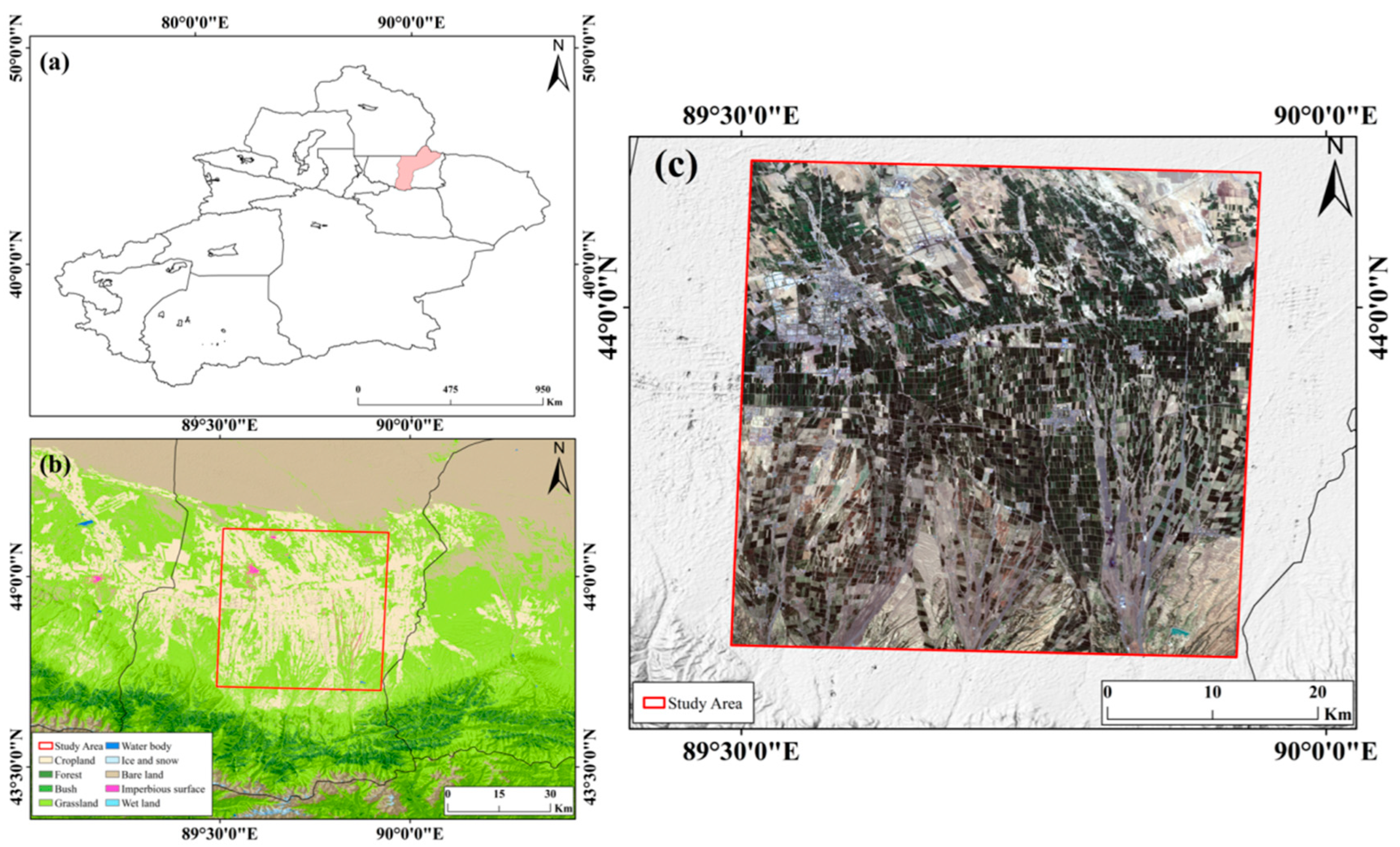
Figure 1. Overview of the study area. (a) The geographical location of Qitai County where the study area is located; (b) the scope of the study area; and (c) an optical remote sensing image of the study area.
Remotesensing 17 03563 g001
Figure 2. CBAM attention mechanism model structure diagram. (a) Diagram of the spatial attention mechanism structure; (b) diagram of the channel attention mechanism structure; (c) diagram of the CBAM attention mechanism structure.
Remotesensing 17 03563 g002
Figure 3. Improved ASPP model structure diagram.
Remotesensing 17 03563 g003
Figure 4. Enhanced U-Net, a semantic segmentation model integrating attention and multi-scale features.
Remotesensing 17 03563 g004
Figure 5. Training loss curves: (a) DeeplabV3+; (b) HRnet; (c) PSPnet; (d) Segformer; (e) U-Net; (f) this experimental method.
Remotesensing 17 03563 g005
Figure 6. Time-series vegetation index map: (a) kNDVI; (b) EVI.
Remotesensing 17 03563 g006
Figure 7. Examples of mapping results from different semantic segmentation models. Black represents background, red represents winter wheat, and blue represents corn.
Remotesensing 17 03563 g007
Figure 8. Wheat and corn extraction results in the study area: (a) the actual distribution; (b) the predicted results.
Remotesensing 17 03563 g008
Figure 9. Test accuracy results for Qitai County.
Remotesensing 17 03563 g009
Table 1. Phenological stages of spring wheat and corn crops.
AprilMayJuneJulyAugustSeptember
EarlyMidLateEarlyMidLateEarlyMidLateEarlyMidLateEarlyMidLateEarlyMidLate
WheatSowing EmergenceJointingTillering HeadingGrain-fillingMilk stage Maturity
Corn Sowing 3-leaf7-leaf Jointing Tillering Milk stage Maturity
Table 2. Confusion matrix. TP is when the model correctly predicts a positive category to be a positive example, FN is when the model incorrectly predicts a positive category to be a negative example, FP is when the model incorrectly predicts a negative category to be a positive example, and TN is when the model correctly predicts a negative category to be a negative example.
Confusion MatrixPrediction
TrueFalse
Ground TruthPositiveTPFN
(True Positive)(False Negative)
NegativeFPTN
(False Positive)(True Negative)
Table 3. Comparison of the accuracy of various semantic segmentation models on the Sentinel-2 RGB dataset.
ModelIoUmIoUPAmPAF1-ScoreOA
WheatCornWheatCorn
Deeplabv3+70.5467.1771.8884.8684.3271.8883.5684.25
PSPnet73.5171.6974.3086.1386.5985.8485.2385.63
HRnet77.0374.5877.8088.4687.9388.0387.4887.94
Segformer61.3159.1465.0074.6778.1378.7778.5979.91
U-Net76.6073.5777.3088.9289.0888.0387.1687.61
Our approach80.3678.6281.3190.4590.5090.1989.6790.07
Table 4. Comparison of the accuracy of various semantic segmentation models on the dataset transformed by Sentinel-2 principal component analysis.
ModelIoUmIoUPAmPAF1-ScoreOA
WheatCornWheatCorn
Deeplabv3+71.3270.8373.1386.6186.7485.4684.4584.94
PSPnet74.8774.5775.6687.8988.4986.9086.1386.36
HRnet78.9078.2879.6190.6390.1089.3488.6488.88
Segformer66.2965.2368.4581.0181.6681.7381.2181.92
U-Net79.3679.2280.4390.6491.3789.8889.1489.41
Our approach82.3782.1683.0392.0792.6891.3490.7390.91
Table 5. Comparison of semantic segmentation models’ performance on the Sentinel-2 principal component transformed dataset.
BaselineCBAMImproved ASPPmIoUF1-Score
80.4389.14
82.8390.61
81.7189.93
83.0390.73
Table 6. Comparison of parameters and computational complexity. Model A is the standard convolution-based ASPP model and Model B is the depthwise separable convolution-based ASPP model.
MetricModel AModel B
Total Number of Parameters191,686,82791,078,827
GFLOPS (Computational load)15.97 G12.75 G
Estimated Memory Usage931.91 MB548.87 MB
Disclaimer/Publisher’s Note: The statements, opinions and data contained in all publications are solely those of the individual author(s) and contributor(s) and not of MDPI and/or the editor(s). MDPI and/or the editor(s) disclaim responsibility for any injury to people or property resulting from any ideas, methods, instructions or products referred to in the content.