High-Throughput UAV Hyperspectral Remote Sensing Pinpoints Bacterial Leaf Streak Resistance in Wheat

Abstract

Bacterial leaf streak (BLS), caused by Xanthomonas translucens pv. undulosa, has become an intermittent yet economically significant disease of wheat in the Upper Midwest during the last decade. Because chemical and cultural controls remain ineffective, breeders rely on developing resistant varieties, yet visual ratings in inoculated nurseries are labor-intensive, subjective, and time-consuming. To accelerate this process, we combined unmanned-aerial-vehicle hyperspectral imaging (UAV-HSI) with a carefully tuned chemometric workflow that delivers rapid, objective estimates of disease severity. Principal component analysis cleanly separated BLS, leaf rust, and Fusarium head blight, with the first component explaining 97.76% of the spectral variance, demonstrating in-field pathogen discrimination. Pre-processing of the hyperspectral cubes, followed by robust Partial Least Squares (RPLS) regression, improved model reliability by managing outliers and heteroscedastic noise. Four variable-selection strategies—Variable Importance in Projection (VIP), Interval PLS (iPLS), Recursive Weighted PLS (rPLS), and Genetic Algorithm (GA)—were evaluated; rPLS provided the best balance between parsimony and accuracy, trimming the predictor set from 244 to 29 bands. Informative wavelengths clustered in the near-infrared and red-edge regions, which are linked to chlorophyll loss and canopy water stress. The best model, RPLS with optimal preprocessing and variable selection based on the rPLS method, showed high predictive accuracy, achieving a cross-validated R² of 0.823 and cross-validated RMSE of 7.452, demonstrating its effectiveness for detecting and quantifying BLS. We also explored the spectral overlap with Sentinel-2 bands, showing how UAV-derived maps can nest within satellite mosaics to link plot-level scouting to landscape-scale surveillance. Together, these results lay a practical foundation for breeders to speed the selection of resistant lines and for agronomists to monitor BLS dynamics across multiple spatial scales.

1. Introduction

Wheat is one of the most economically important crops, providing a staple food for a large proportion of the world’s population. Multiple diseases, incited by fungi and bacteria, threaten the yield and quality of wheat [1]. A disease of emerging concern in the Upper Great Plains of the United States is bacterial leaf streak (BLS) caused by Xanthomonas translucens pv. undulosa. General symptoms of infected plants are water-soaked lesions on leaves that progress to necrotic streaks. The photosynthetic efficiency is reduced by these streaks, leading to impaired grain filling and, hence, yield losses [2]. Generally, yield losses to BLS average below 10%, but they may run as high as 40% when severe outbreaks are promoted by favorable environmental conditions. BLS is considered a seedborne disease; other additional inoculum sources may include crop residues and alternative hosts, primarily grasses [3]. In addition, the secondary spread of this pathogen occurs through wind and rain splash during storm events. The bacterium penetrates the plants through the natural openings, including stomata and wounds, where infection is initiated. Mechanical damage to the wheat plant from hail, wind-blown soil particles, and farming equipment may provide additional avenues for the bacteria to enter the wheat plant. The development of the disease is favored by warm and highly humid conditions; it is generally considered that 10⁸ CFU/mL is the threshold for the bacterial population size that must be reached before symptoms develop. Consequently, environmental conditions play a very important role in BLS epidemiology; good cultural and agronomic practices are required to reduce attacks [2,4].

An integrated approach to the management of BLS is required wherein cultural measures including the rotation of crops, management of crop residues, and use of certified disease-free seeds reduce initial inoculum levels. While moderately resistant varieties have been identified, long-term sustainable solutions through the breeding of resistant cultivars face limitations due to the genetic complexity of resistance. Chemical approaches (e.g., copper-based bactericides) and induced-resistance strategies using chemical inducers have been explored as control options [5,6]; however, these are not commercially feasible means of control because the pathogen may rapidly develop resistance to such chemicals [7]. Similarly, the application of biological control agents has shown variable efficacy that limits the reliable deployment of this method of disease control [7].

The management of BLS is mainly based on choosing cultivars with disease resistance because there are no effective chemical and cultural controls. Conventional methods of diagnosis usually comprise time-consuming visual surveys and laboratory-based tests that are not sensitive enough to provide low-level infection detection [8]. The symptoms of BLS are also quite variable across different wheat cultivars and under varying environmental conditions, further complicating the diagnosis. Regular irrigation, dew, and rain produce high humidity levels that promote bacterial survival and quick growth [9]. The optimum temperature, lying between 15 °C to 30 °C, is normally experienced during wheat growth seasons in several areas; thus, it favors pathogen development. Besides this, the ability of the pathogen to survive in crop residues and alternative hosts has turned BLS into a chronic and serious challenge in many agri-environment systems [10]. It is out of this, plus the inefficiency within most conventional scouting methods, that researchers were able to attempt to take advantage of advanced technological approaches for crop monitoring.

Hyperspectral imaging (HSI) has emerged as a revolutionary technology for agriculture disease monitoring. This technology captures reflectance data from a wide range of the electromagnetic spectrum, which enables detecting slight changes in plant health through changes in pigments, water content, and plant structure [11]. HSI, performed through the use of unmanned aerial vehicles (UAVs), further increases its value through an ability to provide very high-resolution, noncontact assessments across large areas in a short period of time. Such a method reduces time and labor effort for diseases in the field [12,13,14]. The capacity of HSI to detect subtle spectral changes enables the assessment and diagnosis of crop diseases such as BLS.

Some studies prove the potential of HSI for optimization in crop disease detection, which considerably enhances the conventional assessment methodologies based on visuals used in breeding programs to determine resistance. Examples include work by Bauriegel and Herppich, ref. [15] in the hyperspectral and chlorophyll fluorescence imaging of Fusarium infections in wheat, a capability that improves symptom identification that does not become readily visible. Similarly, an investigation of the presence of infection by soil-borne wheat mosaic virus in wheat using HSI was conducted by Haagsma et al. [16], and the potential was highlighted for revealing infections in symptomatic, as well as non-symptomatic, plants. In the context of BLS, HSI has shown promise for assessing infection severity in breeding trials. Cao et al. [17] presented the potential of HSI combined with deep transfer learning for detecting asymptomatic infections of bacterial leaf blight (BLB) in rice. Given the parallels between BLB and BLS, such as the rapid spread under favorable conditions and the importance of resistance for management, methodologies developed for BLB detection could thus be adapted to enhance the evaluation of BLS resistance in wheat breeding programs.

The integration of HSI with UAVs can facilitate timely intervention and management decisions in large-scale agriculture applications. Indeed, previous studies have already shown that UAV-based HSI can monitor several diseases effectively, including wheat stripe rust (Puccinia striiformis), tomato bacterial spots, and citrus canker (Xanthomonas cirtri), through identification of the specific spectral signatures associated with physiological changes in diseased plants. For example, in the case of wheat stripe rust, hyperspectral vegetation indices such as the Modified Green Red Vegetation Index (MGRVI) and Anthocyanin Reflectance Index 2 (ARI2), which were developed using optimal band combinations, were highly effective in quantifying disease severity with high correlation coefficients: R² = 0.746 for MGRVI and R² = 0.755 for ARI2. Advanced regression models, such as multilayer perceptrons (MLPs), further improved the predictive accuracy of disease quantification, thus showing the scalability of UAV-based hyperspectral systems for large-scale field applications [8]. Francesconi et al. [13] demonstrated that the integration of hyperspectral data with thermal imaging has improved the capability of UAV systems to detect diseases such as Fusarium head blight at early infection stages. By capturing specific spectral responses—such as changes in reflectance linked to chlorophyll degradation and water content—alongside physiological indicators like the canopy temperature, these systems have significantly improved detection sensitivity. Such a combination allows the detection of wheat spikes that are affected as early as possible, even under fluctuating environmental conditions. Second, UAV-based HSI systems have improved the employability of VIs in monitoring the health status of crops during various growth stages. RVS1 and GNDVI among others have been able to identify physiological changes such as a decline in photosynthetic efficiency and chlorophyll content caused by the development of wheat rust disease [18]. In parallel, UAV-HSI systems have efficiently monitored disease progression through changes in canopy reflectance. Investigations focusing on stripe rust have derived the best spatial resolutions for the accurate monitoring of the early, mid, and late stages of infection [14]. These advancements highlight UAV-HSI’s pivotal role in scalable and accurate crop disease management. Recent work has moved from vegetation-index correlations toward end-to-end spectral–spatial learning and quantitative regression with UAV-HSI, including pixel-level deep models that directly invert disease severity indices and hybrid CNN–Transformer networks that capture both local and global features [19,20]. Systematic reviews likewise emphasize the surge of UAV-based disease studies, multi-sensor integration, and the need for scalable, interpretable pipelines in breeding and management contexts [21,22]. Parallel advances in UAV–satellite data fusion show how high-resolution hyperspectral maps can be upscaled to platforms like Sentinel-2 for landscape surveillance and time-series monitoring [23,24]. Despite these successes, almost all UAV-HSI studies have targeted fungal pathogens of which lesions produce strong pigment- or water-related spectral shifts. By contrast, BLS symptoms manifest as narrow, water-soaked streaks with subtler and more transient signatures, often confounded with abiotic stress or mechanical injury. This makes BLS harder to detect and has left a noticeable research gap in high-throughput field phenotyping. Against this backdrop, our study contributes an interpretable chemometric workflow that preserves the wavelength meaning and computational efficiency while delivering cross-validated severity estimates for BLS.

Our work fills a critical gap by applying UAV-HSI—with an interpretable chemometric pipeline—to BLS, a disease far less studied than other wheat pathogens. Because BLS is caused by a bacterium rather than a fungus, its epidemiology and lesion physiology differ markedly from rusts and blights; accurate field detection therefore requires bespoke spectral features and calibration strategies. By unifying advanced machine-learning algorithms and spectral-feature-selection techniques, the research has the advantage of addressing the existing high-dimensional data of HSI by substantially reducing the spectral bands, which at the same time, assures high disease detection accuracy. High computation costs are minimized, and operational scalability can be enhanced for such HSI systems. Additionally, this study is unique in its inclusion of BLS, leaf rust, and Fusarium head blight (FHB), with spectral data for each pathogen analyzed separately but unified within a common methodological framework. The purpose of incorporating multiple diseases is not to develop a classification model but to demonstrate spectral differentiation, ensuring that the spectral signature of BLS is distinct. This differentiation strengthens the foundation for the BLS-focused model, confirming that the system can specifically detect BLS while distinguishing it from other pathogens. Unlike previous studies where only one pathogen was analyzed—for example wheat stripe rust [14] or stem rust [18]—the current study examines three diseases independently, thus displaying a further strength of UAV-HSI toward wider applicability in managing diverse wheat diseases. Addressing the gaps in disease management will improve our ability to mitigate economic losses, facilitating greater sustainability in wheat production systems.

2. Materials and Methods

2.1. Experimental Design

The bacterial leaf streak cooperative nursery (BLSCN) was planted on the St. Paul campus of the University of Minnesota on 17 May 2023. The BLSCN, which tests both released and experimental hard red spring wheat lines, was set up in a randomized complete block design with four blocks. The nursery comprised 228 genotypes (228 × 4 = 912 plots); each plot consisted of two 6 ft-long rows spaced 12 inches apart (6 ft × 2 ft). All blocks received identical management: sowing on 17 May 2023, uniform fertilizer and irrigation, and inoculation on 23 June 2023 with strain CIX40 of Xanthomonas translucens pv. undulosa (10⁸ CFU ml⁻¹ in 0.85% NaCl) applied using a gas-powered backpack sprayer producing a fine aerosol [2], a technique proven effective in other field experiments [4]. These practices, together with UAV flights conducted under clear-sky conditions, minimized environmental variability across blocks. Disease severity for BLS was assessed approximately two weeks after inoculation using a 0–9 scale, where 0 = no symptoms and 9 = entire plant infection.

Leaf rust (Puccinia triticina) and Fusarium head blight (FHB; Fusarium graminearum) were studied in separate nurseries. Leaf rust was inoculated in early June using a spreader row of susceptible wheat cultivars and scored on July 17–18 using the modified Cobb scale [25]. FHB was inoculated on 20, 23, 27, and 30 June 2023, by use of a macroconidial suspension of Fusarium graminearum. The FHB severity was assessed on a 0–5 scale.

To ensure consistency across the three pathogens, disease severity scores were transferred to a standardized 0–100 scale (0 = no symptoms, 100 = complete susceptibility). Because each disease has a long-established, pathogen-specific rating system used by our pathology partners, we retained those native scales in the field and then harmonized them computationally. BLS (0–9) and FHB (0–5) scores were linearly rescaled to 0–100, and rust scores from the modified Cobb scale (percent severity plus infection type) were first converted to a 0–9 linearized scale using the published routine of Gao et al. [26] (script available at https://github.com/umngao/rust_scores_conversion (accessed on 9 August 2025)) and then mapped to 0–100. Symptoms used for scoring included water-soaked lesions that turned into necrotic streaks for BLS, rust pustules for leaf rust, and infected spikelets for FHB, following protocols developed for scoring disease severity. 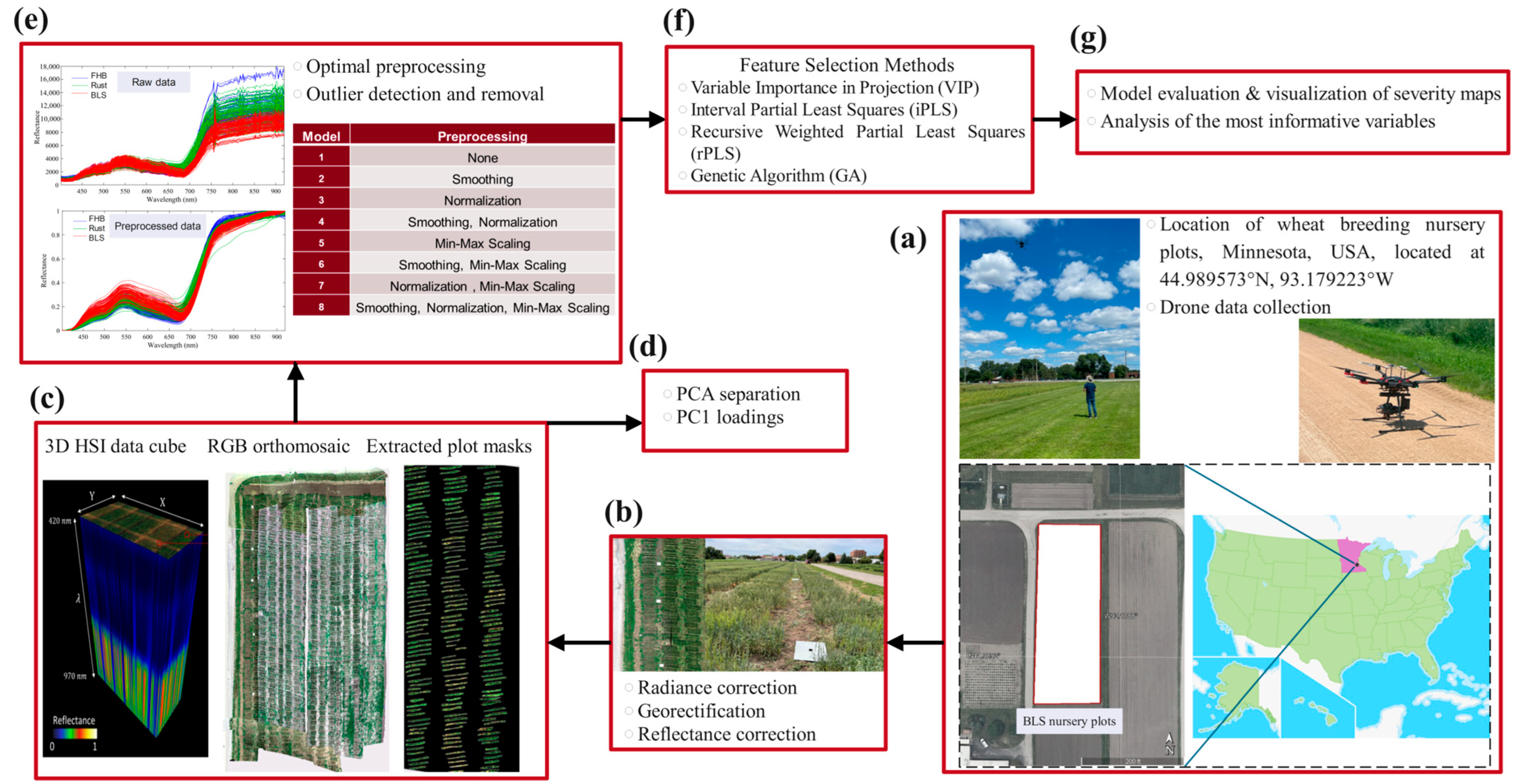The complete acquisition-to-analysis pipeline is outlined in Figure 1.

2.2. Data Collection and Preprocessing

Spectral image data were acquired in the field with a Matrice 600 Pro hexacopter UAV (DJI Inc., Shenzhen, China) equipped with a Resonon Pika L hyperspectral imaging system (Resonon, Inc., Bozeman, MT, USA) (Figure 1). The system was operated with a Resonon NUMI flight computer (version 1.36) and had a 36.5° field of view. The Pika L camera is a push-broom or line-scan imager with a spectral range covering 369.45–1008.65 nm, a spectral resolution of 2.7 nm, and 300 spectral bands. Each 2D image consists of 900 spatial channels; every pixel stores a contiguous reflectance spectrum. The hyperspectral camera system was complemented by an inertial measurement unit (IMU; Ellipse2-N, SBG Systems, Carrières-sur-Seine, France) and a GNSS antenna (TW2410, Tallysman, Inc., Ottawa, ON, Canada) for geolocation and orientation control. The system was stabilized using a three-axis gimbal (Ronin-MX, DJI, Inc., Shenzhen, China). The power supply to both the UAV and the hyperspectral camera was powered by individual lithium polymer batteries.

Autonomous flight missions were conducted with the DJI Ground Station Pro (iOS version 2.0.18). The UAV was programmed to have a flight altitude of 15 m above the ground, with a ground speed of 1.5 m/s, while the ground swath calculated was 9.89 m. Thus, the ground pixel size was about 1 cm. All the flight missions were undertaken during good weather conditions, characterized by a relatively cloudless sky and low wind speeds. Flights were further constrained to a mid-morning window (10:30–12:00 local time) to maintain a stable solar zenith angle and reduce shadowing. The altitude, speed, nadir gimbal orientation, and 36.5° field of view were fixed for every mission, providing consistent viewing geometry and limiting bidirectional reflectance variability. To account for temporal changes in solar illumination, high-density fiberboard white reference panels (60 cm × 60 cm × 3.2 mm) were placed at strategic locations within the experimental area prior to each flight. These panels were imaged for radiometric calibration. The temporally closest panel image was used for each flight line to correct gradual irradiance changes. The low acquisition altitude shortened the atmospheric path length, and bands outside 401.79–918.86 nm—including the strong water-vapor absorption feature near 940 nm—were discarded. Plot spectra were computed by averaging all pixels within each plot, further damping residual directional and atmospheric noise.

Image processing was performed using SpectrononPro software (ver. 3.4.8; Resonon, Inc., Bozeman, MT, USA). First, the raw hyperspectral images were corrected to radiance by using the radiance conversion plugin. Georectification was then performed using synchronized data from the GNSS receiver and IMU, including latitude, longitude, altitude, yaw, pitch, and roll. The corrected radiance images were then transformed to reflectance by using the average measured reflectance of the white reference panels. If an image was missing a reference panel, radiance data from the nearest reference panel in time was used in the conversion to reflectance. Aerial hyperspectral image acquisition was conducted simultaneously with the visual disease severity assessments by the plant pathologists. Hyperspectral signatures were extracted for each two-row plot, providing detailed spectral information on the health and stress conditions of the plants. These spectral signatures were annotated with the corresponding visual disease scores, creating a large dataset relating hyperspectral data to disease severity. To further analyze, the wavelengths at both ends of the original 300-band spectral range were omitted, and a total of 244 wavelengths between 401.79 nm and 918.86 nm were considered. This cutoff was based on empirical inspection of signal-to-noise and reflectance stability: edge bands showed sensor roll-off and atmospheric absorption artifacts, producing noisy, inconsistent values in both white-reference and canopy spectra. Removing these regions reduced distortion in downstream analyses and improved model robustness.

Applying suitable preprocessing techniques in data analysis was important to reduce unwanted variability and improve model performance. Eight alternative pipelines (Models 1–8; Figure 1e) were benchmarked: Model 1 retained the raw spectra; Model 2 applied Savitzky–Golay smoothing; Model 3 applied vector normalization; Model 4 combined smoothing and normalization; Model 5 incorporated Min-Max scaling; Model 6 used smoothing followed by scaling; Model 7 used normalization followed by scaling; and Model 8 applied smoothing, normalization, and scaling sequentially. These algorithms and their combinations were chosen because of their proven effectiveness in hyperspectral studies [27,28]. Each pipeline was implemented before model training to standardize the dataset, suppress noise, and enhance relevant spectral features, thereby improving the predictive accuracy and robustness.

2.3. Modeling and Band Selection

The spectral signatures of BLS, rust, and FHB were analyzed with a total of 300 samples, where 100 samples represented each pathogen, in order to understand the differences between these diseases. In this study, principal component analysis (PCA) was applied as a technique for dimensionality reduction and demonstrated clear separability among the spectral signatures. PCA is one of the common methods for the dimensionality reduction of datasets through linear transformations while preserving the features that contribute the most variance [29,30]. The distribution of principal components provided a good representation of the relationships between spectral variables and sample clusters in multiple dimensions for better discrimination of disease-specific spectral patterns. The analysis here provides a first demonstration of the potential of UAV-HSI data for distinguishing BLS from other diseases in agricultural settings, with each pathogen presenting distinct spectral differences.

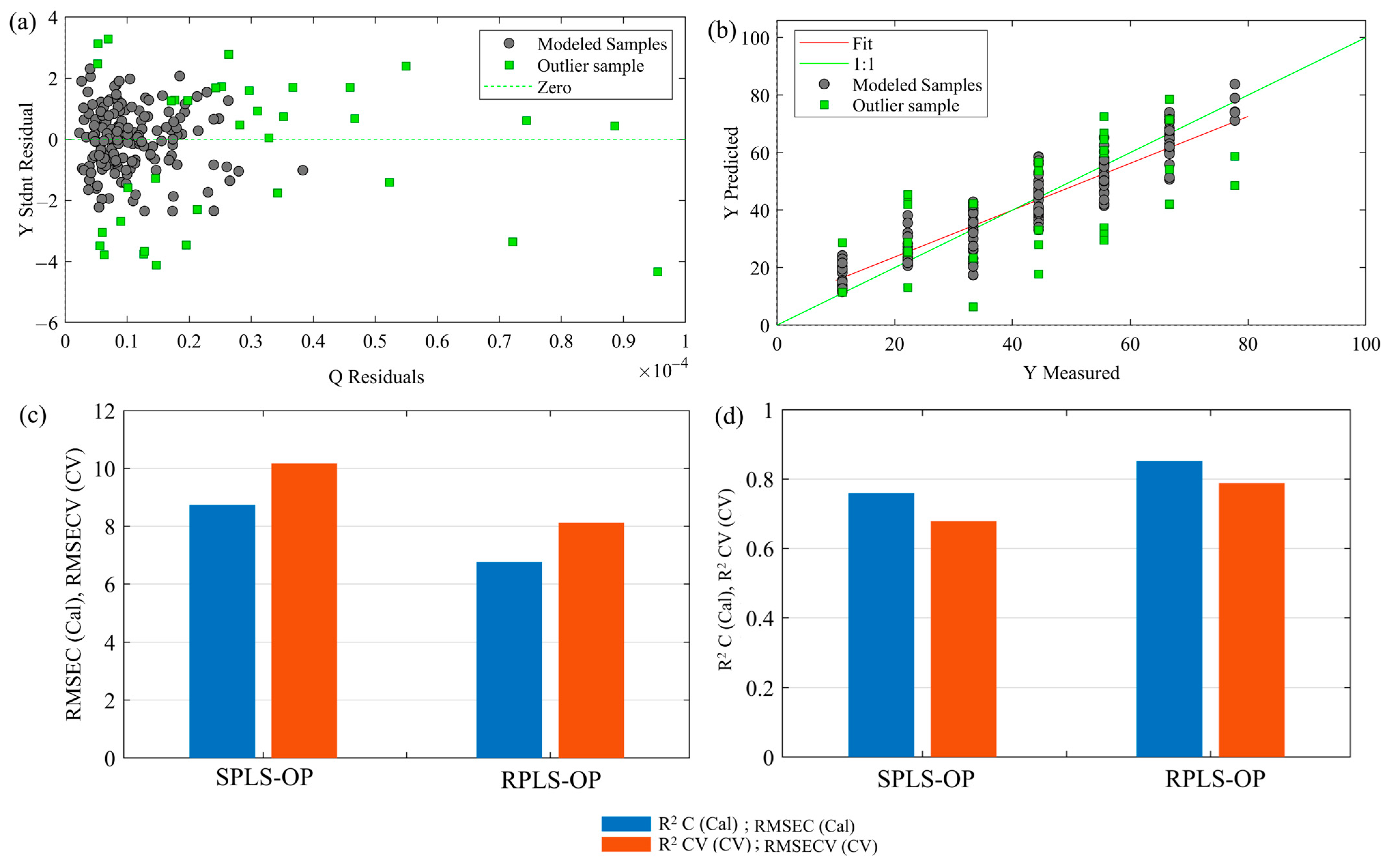
From the 912 BLS plots, a stratified random subset of 200 plots was drawn for model development. Plots were grouped by visual BLS severity (0–1, 2–3, 4–5, 6–7, 8–9), and forty plots were randomly selected from each group while maintaining no more than one plot per genotype per block to preserve the randomized complete block design structure. Partial Least Squares (PLS) regression was then used to build predictive models for BLS in wheat using these 200 samples to relate the spectral data to the visual disease scores, enabling an estimation of disease severity from unique spectral characteristics. PLS is a technique that is popularly known for its efficiency in handling multicollinear datasets by extracting latent variables that explain the maximum variance in the response while reducing redundancy among predictors [31]. The orthogonal latent variables obtained using this method were ranked according to their cumulative contribution, and an accurate and reliable model for BLS detection was built. A robust PLS (RPLS) regression was performed on top of the developed initial PLS models to assure model reliability and decrease the effect of outliers. RPLS extends ordinary PLS by automatically identifying and handling model outliers that are due to measurement errors, biological variability, and mislabeling. Residuals are calculated between predicted and actual values; data points showing very large residuals are tagged as possible outliers. In the process of model calibration, anomalous samples are weighted lower to decrease their influence on the final model [32,33]. This improves the predictive performance of the model but makes it resistant to inconsistencies in data. Further, to enhance the stability and reliability of the model, 10-fold Venetian blind cross-validation was applied. It splits the dataset into 10 distinct splits with a blind thickness of one sample, which provides a robust model evaluation and prevents overfitting. To make the model performance assessment more reliable, this cross-validation approach iteratively trained and validated the model on different subsets of data [34,35].

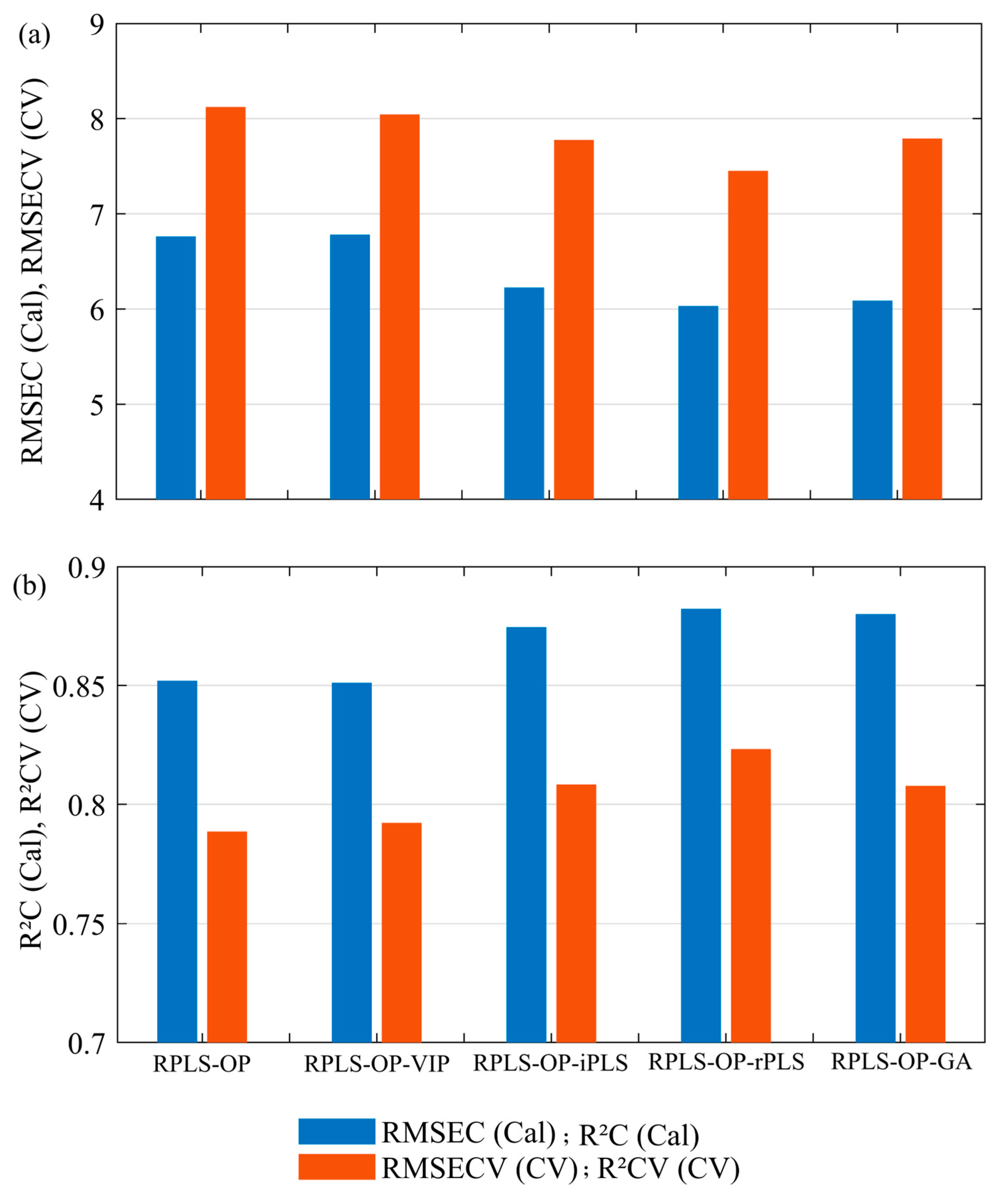
Hyperspectral data are often challenging due to a large number of spectral variables, many of which may be irrelevant or redundant. Variable selection techniques are therefore imperative to optimize model performance by determining the most informative wavelengths, decreasing computational demands, and improving interpretability by focusing on the most relevant spectral features. In the current study, four independent variable selection methods were compared to find the most efficient one: Variable Importance in Projection (VIP), Interval Partial Least Squares (iPLS), Recursive Weighted Partial Least Squares (rPLS), and Genetic Algorithm (GA).

The VIP method was used to rank the spectral variables in the order of their importance to the predictive power of the PLS model. Those variables that have a high VIP score (≥1) are considered important, while low-scoring variables are excluded to simplify the dataset without losing important spectral features. In this work, the VIP scores were calculated iteratively with the removal of a fraction of 0.1 of the variables in each run. This filtering step further refined the dataset and concentrated it on those wavelengths most highly associated with disease detection. iPLS was used for performance assessment over spectral intervals, dividing the range into segments of 11 variables each. In every interval, separate PLS models were developed to which forward mode was applied, adding the intervals in a stepwise manner based on their contribution towards reducing the RMSECV. 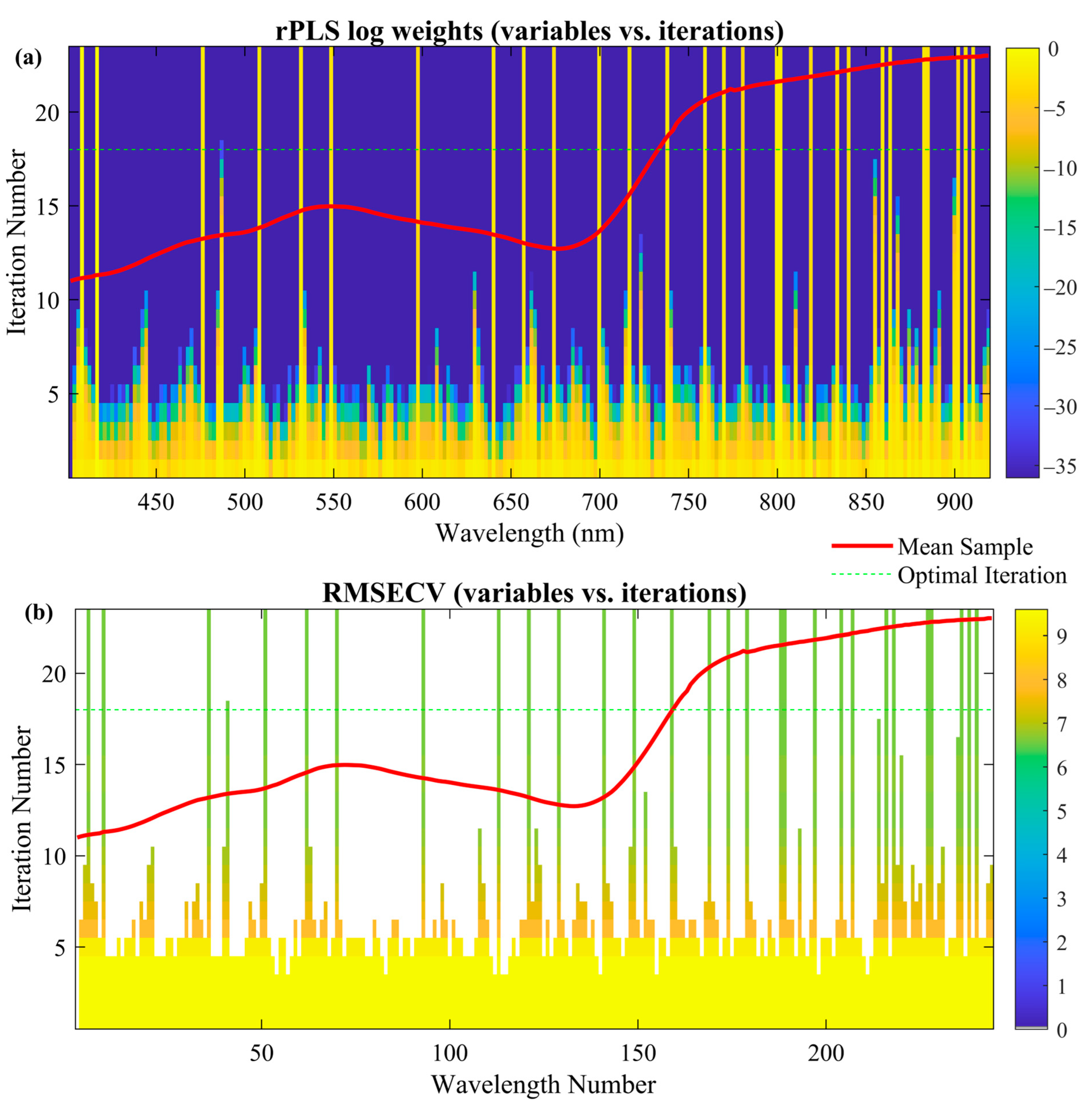This was performed using the stepwise approach, where key spectral regions important for the accuracy of prediction were identified, thus systematically optimizing the model accordingly [34]. rPLS was executed in “surveyed” mode with up to 100 iterations and a maximum of 10 latent variables. All spectral variables enter the first iteration with equal weight; at each subsequent iteration, the normalized absolute regression coefficients from the previous model redefine the weights, progressively down-weighting uninformative bands and emphasizing informative ones. This adaptive procedure dynamically weights spectral variables according to their relevance in the model’s prediction. Variables less useful in the model’s prediction are down-weighted or removed, whereas critical ones receive higher weights, resulting in a leaner and more accurate model [36]. The iterative re-weighting enhances model stability and reduces computational complexity, making rPLS well suited to high-dimensional hyperspectral data. Finally, GA is an iterative method based on the “survival of the fittest” principle. The optimal subsets of variables in GA are identified by the generation and refinement of combinations with the use of fitness through RMSECV, selection, crossover, and mutation. All GA hyper-parameters were tuned through a targeted sensitivity analysis based on cross-validation performance (mutation rates = 0.001–0.020, population sizes = 32–128, window widths = 4–16). The best trade-off between convergence speed and solution quality was obtained with a population size of 64, window width of 8, and mutation rate of 0.005, run for a maximum of 100 generations with double crossover. This configuration provided stable convergence, avoided over-fitting, and efficiently reduced noise and redundancy in the dataset.

For evaluating the performance of the prediction models and finding the best strategy of variable selection, four performance criteria were used: root mean square error of calibration (RMSEC), root mean square error of cross-validation (RMSECV), coefficient of determination for calibration (R²C), and coefficient of determination for cross-validation (R²CV). These metrics could comprehensively assess the model accuracy, generalizability, and stability [31]. In this regard, a comparison was made of the performance of the VIP, iPLS, rPLS, and GA methods in choosing key wavelengths relevant for the detection of symptoms related to BLS. The comparison identified the most efficient method in terms of dimensionality data reduction while preserving the prediction accuracy for an efficient disease-detection system. Each of these techniques has been studied in their ability for isolating relevant spectral features, reducing data processing to improve model stability in BLS detection in wheat.

3. Results

3.1. Pathogen Differentiation Using PCA

Principal component analysis was used to evaluate the UAV-based HSI capability of separating BLS, leaf rust, and FHB spectral data, which were collected separately for each pathogen under distinct field experiments. Each nursery was inoculated with only one pathogen, and plots with any secondary symptoms were excluded, so the PCA reflects single-pathogen spectra rather than mixed infections. By reducing the dimensionality from hyperspectral data with maintained critical features contributing to variances, PCA helps to simplify such complex data by enabling clear visualization of the pattern in spectral data specific to any of the pathogens. A clear separation of the pathogens into clusters can be visibly seen from the result represented in a three-dimensional scatter plot (Figure 2a). PC1 accounted for 97.76% of the total variance and was able to separate BLS from the other pathogens, while PC2 explained 1.92% and PC3 explained 0.22%, further differentiating BLS from leaf rust and FHB. The PC1 loading vector (Figure 2b) shows a strong positive peak near ~680 nm (red-edge onset) and another rise in the NIR around 880–910 nm, with a pronounced negative trough at ~750–780 nm and smaller negatives near 540–570 nm. These spectral zones are tied to the chlorophyll content, leaf structural integrity, and water status—physiological traits perturbed differently by BLS, rust, and FHB—so PC1 primarily encodes these differences, accounting for its high discriminative ability.

These findings agree with the prior work of Bauriegel and Herppich [15], who were able to detect symptoms of FHB based on spectral changes in chlorophyll degradation and water content, identifying distinct wavelengths for monitoring. Likewise, Alisaac et al. [37] have illustrated the efficiency of hyperspectral imaging in distinguishing Fusarium species and grading wheat varieties for the resistance response using spectral vegetation indices together with sophisticated classification techniques. This differentiation highlights the system’s capability to address real-world agricultural challenges involving coexisting pathogens with overlapping spectral signatures. This preliminary classification lays a foundation for the focused analyses of BLS in later sections of this manuscript, as it can be performed with developed models informed by the various distinct spectral behaviors that were highlighted during the PCA analysis. In fact, this step was also important to ensure the system’s capability regarding multipathogen differentiation and for supporting further modeling efforts based on the dataset structure.

3.2. Data Preparation and Model Refinement

3.2.1. Preprocessing Strategies for Enhanced Prediction

Using the pre-processed spectra described in Section 2.2, we compared the eight pipelines (Figure 1e) with respect to calibration (R²C, RMSEC) and cross-validation (R²CV, RMSECV) (Figure 3). The best performance was exhibited by Model 8 with the lowest RMSECV of 10.17 and highest R²CV of 0.678, hence it was named Standard PLS–Optimal Preprocessing because it showed the best accuracy and reliability. This demonstrated how effective the combination of smoothing, normalization, and Min-Max scaling was in noise reduction, data standardization improvement, and consequently improved predictive accuracy of the model.

By comparison, Model 6, with smoothing and Min-Max scaling, was also effective, demonstrating that combined preprocessing strategies work better than the single-step approaches used in Model 2 (smoothing alone) or Model 5 (Min-Max scaling alone). At the other extreme, Model 1 (no preprocessing) produced the poorest result, highlighting the importance of preprocessing in obtaining robust and accurate prediction models. The findings presented above indicate that various preprocessing methods combined, for instance, in SPLS-OP, significantly improved both the reliability and accuracy of BLS severity predictions. In terms of the preprocessing strategy, this will serve as the baseline for hyperspectral data processing forward in this study.

3.2.2. Robust PLS Model for Outlier Detection and Removal

To provide a more robust model and reduce the effect of outliers, RPLS regression was performed. RPLS extends the standard PLS method by identifying and down-weighting outliers based on their residual contributions, so that extreme values caused either by measurement errors or by biological variability do not distort the model. Outliers were flagged when either the sample’s Q-residual exceeded the 95% confidence limit calculated with the Jackson–Mudholkar approximation (as implemented in the robust PLS routine) or the absolute Y-studentized residual was >3.0. Outlier candidates were visualized on the Q-residual vs. Y-standardized residual plot (Figure 4a) and checked on the predicted-versus-measured scatter (Figure 4b); outliers typically deviated from the 1:1 line. Samples exceeding one of the above criteria in the calibration run and again under 10-fold Venetian-blind cross-validation were discarded, yielding 35 outliers (17.5%). This ensured that the modeled samples that remained behind (shaded circles in Figure 4a,b) would contribute to a more reliable and more accurate model.

The performances of the two models were compared: standard PLS with optimal preprocessing (SPLS-OP) and robust PLS with optimal preprocessing (RPLS-OP) (Figure 4c,d). The RPLS-OP model showed better predictive ability, reducing RMSECV from 10.17 in SPLS-OP to 8.12 in RPLS-OP and improving the R²CV from 0.678 to 0.789. These results pointed out that RPLS is effective in handling the outliers and improving the overall robustness of the model.

3.3. Model Development with Selected Variables

The key spectral variables were selected to further improve the predictive accuracy and computational efficiency of the RPLS-OP model identified in the previous section as the optimal model. VIP, iPLS, rPLS, and GA methods were applied to select the most informative spectral bands out of the full set of 244 bands (Figure 5). All these methods reduced the input dimensionality without loss or even with increased predictive power of the model.

The VIP retained 178 variables, which resulted in a spectral band reduction of 27.05%. The selected variables corresponded mostly to red-edge (700–740 am) and near infrared (750–850 am) regions, showing their sensitivity to the chlorophyll degradation and structural changes due to BLS infection. iPLS selectively reduced the input to 44 variables, accounting for an 81.97% reduction by systematically identifying the most useful spectral intervals in terms of predictive contributions. Among them, rPLS selected the most important reduction, preserving only 29 variables, corresponding to a spectral dimensionality reduction of 88.11%. This approach focused on key wavelengths strongly linked to physiological changes induced by BLS. On the other hand, GA selected 56 variables, with a 77.05% reduction, and pointed out broad spectral regions spanning multiple wavelengths. Each method significantly reduced the dimensionality of hyperspectral data while maintaining important spectral information relevant for good predictions. Of these, rPLS had the greatest reduction in spectral bands.

Models developed with selected variables are compared against their performance (Figure 6). The baseline model (RPLS-OP), using all 244 spectral bands, had an RMSEC of 6.763, RMSECV of 8.123, R²c of 0.852, and R²CV of 0.789. The RPLS-OP-VIP model, retaining 178 variables, only marginally improved the cross-validation performance, with an increased the R²CV to 0.792, while the RMSEC went up slightly to 6.782 from the baseline model. The iPLS-based model further improved predictive accuracy by lowering the RMSECV to 7.777 and increasing the R²CV to 0.808. This improvement indicated that high-predictive-relevance intervals were effectively identified using systematic methods with significant variable reduction. The rPLS-based model gave the best results for all the performance indicators with an RMSECV of 7.452 and an R²CV of 0.823. This model focused only on the most informative wavelengths providing robust predictive capability. For the GA-based model, it balanced reduction and performance with a minimum value of RMSECV = 7.792 and an R²CV value of 0.808. Though less effective than the rPLS model, the GA model still appears to be a good choice to identify critical variables from hyperspectral data. Our results suggest that optimizing variable selection approaches improved with the RPLS-OP model, producing models that are simpler to handle with less computational cost.

VIP evaluates single wavelengths within the PLS space and is deterministic and rapid, but it tends to keep strongly collinear bands and thus yields large, partly redundant subsets; iPLS adds or removes contiguous spectral intervals, capturing the local correlation structure yet risking the omission of narrow features that straddle interval edges; rPLS iteratively re-weights variables according to the coefficient stability, concentrating on the most informative bands, but the adaptive weighting can overweight random noise and overfit unless each iteration is cross-validated—as performed here with ten-fold Venetian-blind validation and an early-stopping rule when RMSECV no longer decreased; the Genetic Algorithm explores the search space stochastically through crossover and mutation, escaping local minima and finding parsimonious subsets, though at a higher computational cost and with run-to-run variability. These theoretical considerations explain why rPLS, under strict cross-validation, achieved the best balance between parsimony (29 bands) and predictive accuracy (R²CV = 0.823), whereas VIP retained too many redundant wavelengths and GA reached similar accuracy only after substantially greater computation.

The best model identified for BLS severity prediction in this study was RPLS-OP-rPLS, using the rPLS method for variable selection. The process of variable selection by rPLS is detailed in Figure 7. Successive refinement through iteration helped in the identification of the most informative spectral variables. Figure 7a provides the log weights of variables at each iteration to show how the rPLS method assigned importance to certain wavelengths in a systematic way. Wavelengths with high weights across models within the red-edge and near-infrared parts of the spectrum consistently, between 700 to 740 nm and 750 to 850 nm, were considered in the final model; the critical physiological changes linked to BLS infection fell in these wavelength regions, reflecting chlorophyll degradation and other structural changes within the host tissues. Figure 7b presents the decrease in RMSECV as the rPLS method iterates. The values of RMSECV are high during the first iterations, as some variables are redundant and noisy; afterwards, as the variable set is refined using the iterative algorithm, RMSECV decreases and stabilizes at a minimum value, considered to be optimal for the final subset of variables. This demonstrated the capability of rPLS to enhance model robustness and predictive accuracy by excluding irrelevant data. The rPLS model used in this work allows for complete exploration; thus, the “surveyed” mode was taken into consideration, which contemplates a range of latent variables with a maximum number of 100 iterations. In such a way, it guaranteed that the selection of variables was thorough, identifying the most relevant spectral intervals with the least noise. This systematic refinement is complemented by cross-validation, whereby the rPLS method balances the two contrasting objectives of dimensionality reduction and model performance.

This approach agreed with previous studies examining the performance of rPLS for variable selection in spectral data analysis. For instance, Li et al. [38] applied the rPLS to a dynamic online learning model, which improved the accuracy of near-infrared spectroscopy-based fat content detection for Korean pine nuts. Their approach iteratively refined the feature set and thereby substantially improved prediction accuracy. This emphasizes the ability of rPLS to deal with evolving datasets and complex spectral data. Similarly, in precision viticulture, Benelli et al. [39] applied rPLS for automating the selection of key regions of interest in hyperspectral images of grapevines. This enabled the effective prediction of the soluble solid content in grapes with high sensitivity and specificity, while demonstrating that rPLS can be scaled up for field applications.

Additionally, Cruz-Tirado et al. [40] showed the efficiency of rPLS in reducing redundancy and optimizing predictive models of protein and lipid content in black soldier fly larvae in flour using portable NIR spectroscopy. Blas Saavedra et al. [41] applied rPLS to NIR hyperspectral imaging for the prediction of physicochemical properties in Cape gooseberries by enhancing the regression performance through the selection of relevant spectral variables. Similarly the work of Mancini et al. [42] applied rPLS to predict the soluble solid content in strawberry and in relating selected wavelengths to fungal tolerance. Wang et al. [43] validated the applicability of rPLS to quantify polysaccharide contents in shiitake mushroom beverages; the model obtained a predictive R² above 0.95, demonstrating how robust the application of the rPLS method is in avoiding superfluous wavelengths.

This application of rPLS in this study, demonstrating a high coherence between rPLS-selected wavelengths and physiological markers of BLS, further corroborates earlier findings, reinforcing its strength in the selection of spectral variables. rPLS balances the trade-off between dimensionality reduction and model performance through cross-validation. It ensures an efficient search within the spectral data and gives scalability to UAV-based hyperspectral imaging frameworks.

4. Discussion

4.1. Analysis of the Most Informative Variables

The 29 selected wavelengths based on the rPLS method were further evaluated and ranked using Spearman correlation and mutual information. Spearman correlation gives a measure of the strength and the direction of the monotonic relationship between two variables. Actually, it is most useful in capturing nonlinear relationships—a common feature in hyperspectral data. Mutual information, on the other hand, is a measure of the amount of information that is shared by two variables and is used to identify complex dependent relationships that can be hidden by the standard correlation measures. Thus, taking both measures together provides an overall assessment of the informativeness of all wavelengths. Using these metrics, the wavelengths were ranked to identify the most critical ones for predicting BLS severity. 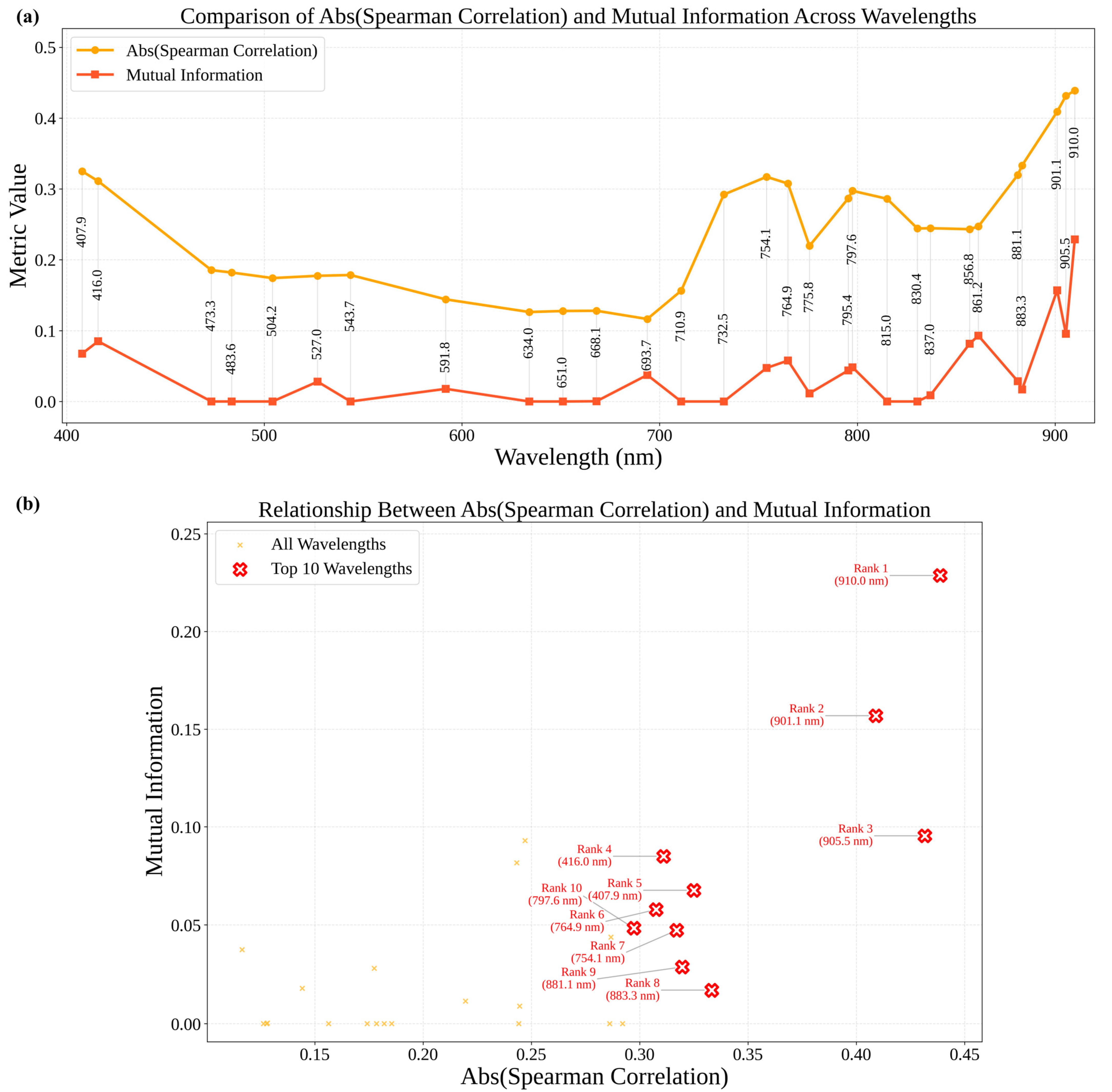Figure 8 provides a comparison of selected wavelength values of Spearman correlation and mutual information.

Figure 8a presents the absolute Spearman correlation and mutual information values across the selected wavelengths. From this data, it is evident that some of these wavelengths, especially those in the near-infrared (910.0 nm and 905.5 nm), are characterized by very high values for both, reflecting a strong relationship with BLS severity and large information content. Most of the wavelengths in the visible part generally exhibited low values, which reflected relatively weak relationships with BLS severity. The relative position of the wavelengths based on the absolute values of Spearman correlation and mutual information is given in Figure 8b which is also complemented by ranking and annotating the ten most informative wavelengths. The optimal wavelengths are generally located in the near-infrared and red-edge regions, thus emphasizing their potential role in identifying physiological changes in the host plant due to BLS. For example, the wavelength 910.0 nm achieved the highest values for both metrics, making it the most critical variable for the model. Similarly, the 901.1 nm and 905.5 nm wavelengths are the second and third most informative wavelengths, respectively.

The wavelengths that correspond directly to the physiological changes induced by BLS likely reflect the reduction in water content, change in structural composition, and other physical damage to leaf tissues. Recent studies on bacterial diseases report the same pattern. In tomato bacterial wilt [44], near-infrared reflectance decreases while visible reflectance increases, and in rice bacterial leaf blight [45], UAV hyperspectral imaging has detected both symptomatic and asymptomatic infections. In addition, Deng et al. [8] also confirmed NIR and red-edge bands as effective for enhancing vegetation indices’ performance, such as the Red Edge Disease Stress Index, where high accuracy—R² = 0.79—was achieved by identifying wheat stripe rust severity. These results emphasize further that these spectral regions are essential in the remote detection of infections caused by a wide array of plant pathogens.

The red-edge region is highly valuable for the detection of photosynthetic stress and chlorophyll degradation. Spectral shifts in this range reflect changes in the pigment content and canopy structure, which are critical indicators of disease progress. Metrics such as the normalized reflectance indices, for example, NRI680/850 and NRI700/850, effectively combine NIR and red-edge bands to discriminate between bacterial and viral infections and thus allow early and correct disease detection [46].

Bevers et al. [47] also indicated that these spectral regions are useful for diagnosing viral infections in maize, such as the highly economically impactful sugarcane mosaic virus disease. Their study revealed how both NIR and red-edge wavelengths enhance model accuracy, thereby enhancing the detection of infection-induced changes in leaf physiology. Likewise, a hyperspectral study on downy mildew in Brassica oleracea found that red-edge and near-infrared-based indices were the most sensitive to disease severity, outperforming conventional visible-band indices [48]. All these studies give validation to the importance of those spectral regions for the detection of diseases in crops.

This study reinforces the key roles of NIR (e.g., 910.0 nm, 905.5 nm) and the red-edge (700 to 740 nm) in hyperspectral imaging, in relation to BLS monitoring, for the detection of changes related to plant structure, water, and photosynthesis. These should be incorporated into UAV-based hyperspectral image frameworks to develop appropriate, efficient, and scalable solutions for breeding wheat with improved resistance.

4.2. Visual Insights and Exploring Integration with Satellite Data

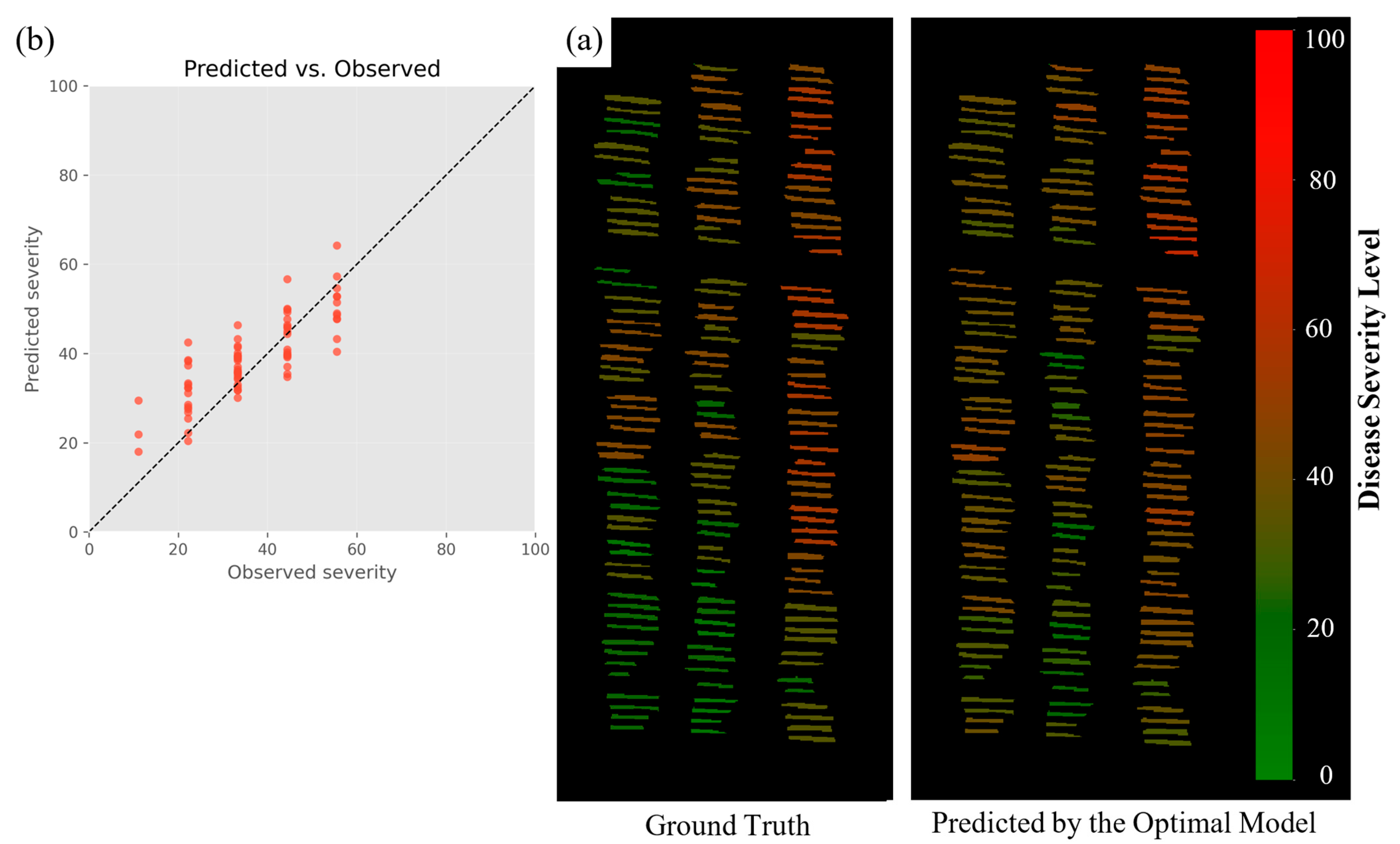
Figure 9 shows model predictions for a hold-out subset of plots from the 2023 St. Paul nursery that were not used for calibration; all plots were flown and visually scored on the same day under identical management and illumination conditions. Figure 9a compares ground-truth (left) and predicted (right) severity maps. Each short bar represents one two-row plot, colored from green (low BLS severity) to red (high severity) on the 0–100 scale, enabling a direct, spatially coherent comparison between field scores and model estimates. Figure 9b summarizes the same data in a predicted-versus-observed scatter; the dashed 1:1 line marks perfect agreement, and the model achieved an RMSE of 7.60 disease-index units. This visualization is especially useful for plant breeders because it allows them to draw practical conclusions on the susceptibility and resistance reactions of wheat lines. By analyzing the gradients in disease severity across experimental plots, breeders can identify those resistant varieties that showed minimal symptoms under similar pathogen pressure. This will facilitate the prioritization of such lines for further genetic and phenotypic studies, hence optimizing the breeding program’s ability to accelerate the development of disease-resistant cultivars. Finally, and most importantly, the model is scalable to larger plots and across agroecosystems, since the model can work with external data. When combined with UAV-based hyperspectral imaging, breeders can screen numerous wheat lines with fine levels of spatial and temporal detail. This approach reduces some of the limitations of satellite-based data by providing high-resolution, plot-level information that satellites cannot provide. The models bridge satellite to UAV imaging, transitioning breeders from broad landscape screening to precise plot-level evaluations. High predictive power and visualization, as realized in Figure 9, make the model an important tool in furthering wheat breeding and improving disease-management strategies.

The wavelengths selected by the rPLS method span key spectral regions, near-infrared, red-edge, and blue, offering diverse and complementary insights into BLS severity. These wavelengths align with Sentinel-2 satellite data bands while also extending into finer spectral details that satellites cannot capture.

Critical wavelengths in the NIR region (~800–910 nm) are 910.0, 905.5, 901.1, 883.3, and 881.1 nm, showing the highest mutual information and Spearman correlation values with BLS severity. These bands provide information on structural changes and the water content in vegetation. Thus, 910.0 nm (Rank 1), 905.5 nm (Rank 3), and 901.1 nm (Rank 2) are bunched around Sentinel-2 Band 8A (865 nm), both pointing out their potential in vegetation stress detection. The relatively small offset of the Sentinel-2 bands with respect to the UAV-based optimal wavelengths would hint that UAV systems could capture more detailed information in this range, complementing satellite observations. Wavelengths 883.3 nm (Rank 8) and 881.1 nm (Rank 9) are closer to Sentinel-2’s Band 8, at 842 nm, which also gives useful information on vegetation health, though with less precision compared to UAV hyperspectral imaging. The Red-Edge region (~700–780 nm) is sensitive to chlorophyll content and stress responses and includes wavelengths such as 764.9 nm (Rank 6), 754.1 nm (Rank 7), and 797.6 nm (Rank 10); these are proximal to Sentinel-2’s red-edge bands (Bands 5, 6, and 7 at 705 nm, 740 nm, and 783 nm, respectively). While these bands provide a broad overview of the vegetation condition, UAV-selected wavelengths refine this to specific stress responses.

The wavelengths in the blue region (~407–416 nm) are notably 407.9 nm (Rank 4) and 416.0 nm (Rank 5), showing strong relationships with BLS severity. These are rather shorter than the blue band of Sentinel-2, which is 490 nm, and thus indicate extra valuable information that UAV-based hyperspectral imaging captures about pigment-level changes and subtle early stress signals not evident in satellite data.

The correspondence of UAV-selected wavelengths with Sentinel-2 bands underlines the possibility of satellite and UAV data integration. The broader NIR and red-edge bands of Sentinel-2 (Band 8A and Band 8) enable an efficient, large-scale overview of vegetation health by identifying areas that might be under stress. Value addition by the UAV hyperspectral system is the finer spectral resolution in these regions, hence enabling detailed analysis of stress-specific signatures, especially in the NIR range of 901–910 nm and the red-edge region of 754–765 nm. In addition, UAV-based measurements give unique insights in the blue region, which are not captured in Sentinel-2 data. This is a complementary approach toward multi-scale monitoring, where Sentinel-2 could give an initial large-scale screening, while UAV-based hyperspectral imaging provides precision monitoring in areas of concern. Therefore, the strengths of these platforms are combined to further enhance the accuracy, efficiency, and scalability of precision agriculture practices. No Sentinel-2 pixels were used in model calibration or validation; the comparison was limited to wavelength alignment. To operationalize this integration, the UAV cube used here resolves ≈1 cm pixels with 2.7 nm spectral bands, whereas Sentinel-2 delivers 10 m pixels and ~15–20 nm bands (for example, Band 8A is centered at 865 nm with a full width at half maximum of 20 nm). UAV spectra can be aggregated to 10 m × 10 m tiles, and each tile spectrally convolved with the published Sentinel-2 response functions, producing a spatial–spectral stack directly comparable to Sentinel-2. This allows Sentinel-2 to provide broad coverage, while UAV data supply plot-level detail for calibration and validation.

5. Conclusions

The presented work was intended to explore the use of UAV-based HSI for the quantification of BLS in wheat and to establish its difference from other important co-occurring diseases, including leaf rust and FHB. This study used advanced machine learning and spectral data-analysis methods to identify the efficiency of hyperspectral data in reflecting subtle physiological changes linked to disease severity. Some of the preprocessing techniques, robust Partial Least Squares regression, and variable selection methods were identified as important for enhancing model accuracy and efficiency. rPLS was the best variable selection method, reducing the number of spectral bands from 244 to 29 while maintaining high predictive accuracy (R² = 0.823, RMSECV = 7.452). These selected wavelengths, especially those in the near-infrared and red-edge regions, are strongly associated with disease-induced physiological changes such as chlorophyll degradation and water stress.

The integration of UAV-derived hyperspectral imaging with visual assessments provided plot-level precision, allowing breeders to identify disease-resistant wheat lines effectively. Furthermore, the correspondence of the selected UAV wavelengths to Sentinel-2 satellite bands underlined the possibility of multiscale disease monitoring, combining the fine resolution of UAV imagery with broad-scale assessments of satellite systems.

The standardized severity gradients across plots directly supports breeder decisions—lines showing minimal symptoms under comparable pathogen pressure can be prioritized for genetic and phenotypic follow-up. Building on this foundation, transitioning to field-ready use requires (i) embedding the workflow in routine breeding and pathology programs, (ii) defining severity thresholds that guide breeding selections and inform cultural management actions (e.g., targeted scouting, roguing infected plots, crop-rotation planning, use of certified seed), and (iii) automating alerts/prescription outputs for rapid deployment. Given the absence of effective chemical control options, these integrations ensure that the spectral pipeline delivers actionable value. The model’s scalability—from plot to field and across agroecosystems—and its computational efficiency enable near real-time assessments, bridging broad satellite screening with precise UAV-level interventions. Although the present study demonstrates strong performance, its scope was confined to a single site and season, relied on a research-grade hyperspectral sensor, and generated plot-scale predictions only. Future work will extend the dataset across additional seasons and sites, evaluate lower-cost narrow-band sensors guided by the key wavelengths identified here, and fuse our plot-level predictions with RGB and LiDAR layers—while developing routines for mixed-symptom disentanglement—to streamline adoption at commercial scales. This work therefore reinforces UAV-HSI as a scalable, reliable platform that can drive a paradigm shift toward resource-efficient breeding and precision disease management.