Building Outline Extraction via Topology-Aware Loop Parsing and Parallel Constraint from Airborne LiDAR

Highlights

What are the main findings?

• Boundary point extraction is formulated as a topology-aware loop searching and parsing problem, enabling automatic identification of erroneous boundary points.
• A dominant direction detection method based on angle normalization, merging, and perpendicular pairing is proposed, and building outlines are regularized under the parallel constraint according to the unit length residual metric.

What is the implication of the main finding?

• We propose a robust and accurate solution for boundary point extraction, dominant direction detection, and outline regularization.
• The proposed method can provide accurate and regularized building outlines for building 3D reconstruction and related applications.

Abstract

Building outlines are important vector data for various applications, but due to the uneven point density and complex building structures, extracting satisfactory building outlines from airborne light detection and ranging point cloud data poses significant challenges. Thus, a building outline extraction method based on topology-aware loop parsing and parallel constraint is proposed. First, constrained Delaunay triangulation (DT) is used to organize scattered projected building points, and initial boundary points and edges are extracted based on the constrained DT. Subsequently, accurate semantic boundary points are obtained by parsing the topology-aware loops searched from an undirected graph. Building dominant directions are estimated through angle normalization, merging, and perpendicular pairing. Finally, outlines are regularized using the parallel constraint-based method, which simultaneously considers the fitness between the dominant direction and boundary points, and the length of line segments. Experiments on five datasets, including three datasets provided by ISPRS and two datasets with high-density point clouds and complex building structures, verify that the proposed method can extract sequential and semantic boundary points, with over 97.88% correctness. Additionally, the regularized outlines are attractive, and most line segments are parallel or perpendicular. The RMSE, PoLiS, and RCC metrics are better than 0.94 m, 0.84 m, and 0.69 m, respectively. The extracted building outlines can be used for building three-dimensional (3D) reconstruction.

1. Introduction

Buildings are the most important constituent elements of the city, and their outlines are widely used for building three-dimensional (3D) reconstruction [1], building urban planning [2], and urban disaster analysis [3]. Because of its ability to acquire accurate 3D point clouds, airborne light detection and ranging (LiDAR) has been widely used for building outline extraction. In the process of outline extraction, boundary points need to be extracted first, and then regularized to generate outlines.

However, due to the inherent deficiencies of point clouds (e.g., uneven point density and insufficient sampling) and complex building structures, extracting satisfactory building outlines from scattered LiDAR point cloud data remains a challenging task. In the paper, a building outline extraction method based on topology-aware loop parsing and parallel constraint is proposed. The main objectives of this study are: (1) to automatically extract semantic boundary points and eliminate erroneous boundary points; (2) to reduce the impact of scattered point clouds on dominant direction detection and obtain accurate dominant directions; (3) to introduce more precise metrics to evaluate the matching degree between dominant direction and the line segment to be adjusted during the outline regularization.

The main contributions of the proposed method can be summarized as follows:

(1) For most existing boundary point extraction methods, it is a challenging task to recognize erroneous boundary points due to uneven point density, data missing, and unreasonable parameters. To solve the issue, we formulate boundary point extraction as a topology-aware loop searching and parsing problem. Semantic loops are detected from an undirected graph, and erroneous boundary points are identified by parsing the geometric characteristics of the semantic loops.

(2) Unlike most existing methods that simply merge possible dominant directions to obtain dominant directions, a method based on angle normalization, merging, and perpendicular pairing is proposed. The proposed method fully exploits the potential parallel and perpendicular relationship between possible dominant directions and merges them in a bottom-up manner to obtain accurate dominant directions.

(3) Unit length residual metric is proposed to select the optimal dominant direction for line segments to be adjusted during outline regularization. The metric simultaneously considers the fitness between the dominant direction and boundary point distribution, as well as line segment length.

The remainder of the paper is structured as follows. Section 2 is a review of related work on building outline extraction. Section 3 describes the methodology, including boundary point extraction and outline regularization. Section 4 presents and analyzes the experiments. Section 5 discusses this article. Finally, Section 6 concludes the study.

2. Related Work

Over the past few decades, numerous research efforts have focused on building outline extraction, and a wide range of methodologies have been proposed. Below is a comprehensive overview of the approaches regarding boundary point extraction and outline regularization.

2.1. Boundary Point Extraction

Existing boundary point extraction methods can be broadly categorized into five main approaches: image-based method, triangulation-based method, feature-based method, Alpha Shapes method, and learning-based method [4,5,6].

2.1.1. Image-Based Method

For the image-based method, 3D unorganized points are first projected onto regular two-dimensional (2D) grids or cells to generate images. Boundary points are subsequently extracted by processing the images using the classical image processing operators [4], e.g., Canny [7], Sobel [8], and Roberts [9]. In Ref. [10], binarized images were generated by projecting points into grids, where grid intensity values were assigned as 0 or 1 based on point distribution. Then, boundary grids were identified by analyzing the point distribution of neighborhood grids. Points inside the boundary grids were classified as boundary points. To mitigate the influence of grid size on extraction results, in Refs. [11,12], grid size was set according to the length and width of the minimum bounding rectangles of the point clouds.

The image-based method is often efficient and can process massive point clouds. However, some salient defects cannot be ignored. First, compared with other methods, scattered points are first converted into images, and some information of the original point clouds is inevitably lost during the process [4], which reduces the accuracy of boundary point extraction. Second, it is difficult to determine an appropriate grid size for the scattered points, and the extracted boundary points are usually of low accuracy and require refinement through post-processing [6].

2.1.2. Triangulation-Based Method

Triangulation-based method constructs topologically structured triangular meshes using scattered point clouds and extracts boundary points by analyzing the triangular meshes. In [13], Delaunay triangulation meshes were generated under the side length constraint. The sides shared by only one triangle were then identified as edges, and corresponding points were identified as boundary points. In Ref. [14], a modified Delaunay triangulation was constructed under the side length, aspect ratio, and interior angle constraints. Then boundary points were extracted based on the sum of vertex angles. Because triangular meshes of large datasets demand substantial computational resources, in Ref. [6], only coarse boundary points extracted by the image-based method were used to construct triangulation meshes. However, only outer boundary points were extracted.

Triangulation-based method can extract concise boundary points, but the extraction results are sensitive to mesh quality. In practice, due to the scattered point clouds and unreasonable parameters, it is easy to generate abnormal triangles, and they cannot accurately depict the shape of the point clouds. As a result, non-boundary points are prone to being misidentified as boundary points, and it is a challenging task to automatically identify these erroneous boundary points.

2.1.3. Feature-Based Method

Unlike image-based and triangulation-based methods, the feature-based method does not require projecting point clouds onto 2D grids or constructing topological structures between points. Instead, it directly extracts boundary points by analyzing local neighborhood distribution, because the neighborhood distribution of boundary points is different from that of non-boundary points. In Ref. [15], point clouds were first divided into multiple bands with the same directions, and two points with the farthest Euclidean distance were regarded as boundary points. In Refs. [16,17], angles between the adjacent vectors formed by the neighborhoods were calculated, and one point was identified as the boundary point if the maximum angle exceeded the predefined threshold. In Ref. [18], the average point spacing of the neighborhoods was designed to recognize boundary points since the average point spacing of boundary points was larger than that of non-boundary points. In Ref. [19], point clouds were projected onto horizontal cells, and boundary points were extracted by analyzing the distribution of cells. Because extracted boundary points of the feature-based method are redundant and nonsequential, in Ref. [20], coarse boundary points were refined by constructing and analyzing the triangulation. However, the process was complex, and only outer boundary points could be extracted.

Although the feature-based method can rapidly extract boundary points, it is very difficult to select reasonable thresholds to reduce the impact of uneven point density. In addition, the absence of sequence relationships between extracted boundary points prevents the generation of outlines, increasing the workload in subsequent stages.

2.1.4. Alpha Shapes Method

Alpha Shapes method has been widely used for boundary point extraction due to its ability to extract boundary points from arbitrary-shaped point clouds. Compared with other methods, the Alpha Shapes method extracts boundary points simply by analyzing the value of the rolling circle radius α [21]. The time complexity of determining whether a point is a boundary point is $O\left(n^3\right)$ [22]. To improve its efficiency, in Ref. [23], coarse boundary points were first extracted using the image-based method. Then, the coarse boundary points were refined using the Alpha Shapes method. In Ref. [24], boundary points were traced and extracted from the neighborhoods of the current boundary point seed, and algorithmic efficiency was significantly improved. Since the parameter α directly determines the level of detail in boundary extraction, many studies have been done on the parameter α. In Refs. [25,26], parameter α was calculated using the average point spacing of neighborhoods. In Ref. [27], two different α values were used to reduce the impact of point density variation. Boundary points with different details were obtained, and accurate boundary points were obtained via refinement. In Ref. [28], a method combining five different strategies was used to estimate the parameter α, and the boundary points occluded by vegetation could also be successfully extracted.

Compared with other methods, the Alpha Shapes method can extract compact and sequential boundary points from arbitrary-shaped point clouds, but two main defects cannot be ignored. (1) The time complexity is much higher than that of other methods, which means that the Alpha Shapes method is not suitable for directly processing large-scale point cloud data. (2) Alpha Shapes method is sensitive to the parameter α, and it is easy to extract erroneous boundary points. How to automatically recognize these erroneous boundary points remains a challenge.

2.1.5. Learning-Based Method

With the rapid development of machine learning, many researchers have utilized machine learning methods to extract boundary points. Compared with non-learning-based methods, this method requires pre-collecting labeled samples and then extracting features to train a machine learning model. After training, the model is used to predict boundary points [29,30,31]. According to the feature extraction approaches, the learning-based method is divided into deep learning-based method and conventional machine learning-based method. For the deep learning-based method, features are automatically extracted. In recent years, deep learning-based methods, e.g., EC-Net [29], EDC-Net [30], and 3D-GMCGAN [31] have been proposed. In Ref. [29], PointNet++ was used to extract multi-scale feature vectors, then boundary points were predicted by constructing a distance distribution regression from each point to the edges. In Ref. [30], point features were extracted using a capsule network, and then a weakly supervised transfer learning strategy was employed to detect boundary points and address the issue of lacking annotated training data. For the conventional machine learning-based method, features (e.g., angular difference, curvature, and normal vectors) are first manually designed based on local neighborhood distribution [16,17]. Subsequently, trained conventional classifiers, e.g., Random Forest [32] and Support Vector Machine [33], and manually designed features are employed to extract boundary points

Learning-based method can extract boundary points, but the extracted boundary points are relatively rough and lack topological relationships, which increases the difficulty of generating outlines [4]. Moreover, training the model requires training datasets, and the labeling process is time-consuming.

2.2. Outline Regularization

Outlines generated directly from original boundary points are often jagged and cannot accurately depict the shape of buildings. Therefore, it is necessary to simplify and regularize boundary points. Many researchers have investigated outline regularization methods, which can be broadly categorized into three main methods: origin points selection-based method, dominant direction-based method, and optimization-based method [5,13,24].

2.2.1. Origin Point Selection-Based Method

Origin point selection-based method generates outlines by selecting key points from extracted boundary points. A typical representation is the Douglas-Peucker algorithm (DP) [34], which iteratively preserves points whose perpendicular distance to the baseline exceeds the predefined threshold. In Ref. [35], the DP method selected key boundary points, which were then used to form building outlines. In the sleeve-fitting algorithm [36], key points within a preset band width were retained, while other points were discarded. Subsequently, endpoints and turning points within the band were used to generate outlines. In the turning function algorithm [37], the turning angle function captured the cumulative turning angles along the boundary points. Key points were identified based on significant changes in the turning angle function. In Ref. [38], boundary points were transformed into one-dimensional signals, and key boundary points were identified by analyzing the denoised signals.

Although the origin point selection-based method can efficiently detect key boundary points, compared with other methods, the generated outlines are unattractive because line segments formed by the critical points are neither parallel nor perpendicular. Additionally, in practice, outline corners may not perfectly align with any point clouds due to uneven point density distribution, leading to missing key points at outline corners.

2.2.2. Dominant Direction-Based Method

The dominant direction-based method sequentially adjusts line segments according to the predefined rules. In Ref. [39], the longest line segment was used to calculate the dominant direction, and other line segments were then adjusted to be parallel or perpendicular to the dominant direction using the hierarchical least-squares solution. In Ref. [40], long line segments were utilized to estimate dominant directions. For each line segment, the angle between it and the dominant direction was calculated. Then, the line segment was adjusted to be parallel, perpendicular, or unchanged according to the angle. In Ref. [41], the bounding rectangle with the maximum number of boundary points was selected as the minimum bounding rectangle (MBR), and all line segments were adjusted to be parallel or perpendicular to the MBR. To extract occluded building outlines, in Ref. [42], boundary points located in the occluded regions were excluded during the MBR generation, and then the missing outlines were recovered using the MBR. Although the MBR-based method can extract attractive and smooth outlines, not all buildings are rectangular in shape, which limits the practicality of the MBR method.

Dominant direction method can extract satisfactory outlines that conform to human vision cognition, but most methods limit the number of dominant directions, which is not suitable for complex buildings with multiple dominant directions. In addition, the accuracy of dominant directions significantly influences the quality of the regularized outlines. However, due to the scattered point clouds, extracting accurate dominant directions from complex buildings is still a challenging task.

2.2.3. Optimization-Based Method

Optimization-based method converts outline regularization into an objective function optimization problem that integrates prior knowledge. Compared with other methods, the optimization-based method simultaneously adjusts all line segments by optimizing the objective function. In Ref. [43], line segments and dominant directions were first obtained, and then an energy function composed of neighbor smoothness and data fitting degree was constructed. Subsequently, the energy function was optimized and each line segments were adjusted according to the assigned dominant direction. Similarly, in Ref. [24], the energy function consisted of a data term and a smooth term. The data term measured the degree of matching between the dominant direction and the line segments, while the smooth term was used to exploit the contextual relationships between line segments. In Ref. [44], line segment adjustment was transformed into a multi-label problem, and the objective function included data term, smooth term, and label term. Similarly, in Ref. [45], the energy function consisted of the distance term, angle term, and length term.

In summary, the optimization-based method is flexible by incorporating prior knowledge into the regularization process and often obtains globally optimal results [5,46]. However, it is difficult to design an appropriate objective function that balances prior knowledge and boundary points, and the weights of different terms significantly affect regularization results. In addition, the optimization-based method is complicated and time-consuming during the process of constructing and optimizing objective functions.

3. Methodology

The proposed method mainly consists of three steps: boundary point extraction, dominant direction detection, and outline regularization. The algorithm workflow is shown in Figure 1.

3.1. Boundary Point Extraction

3.1.1. Constrained Delaunay Triangulation (DT)

Before boundary point extraction and outline regularization, 3D building points are projected onto the horizontal plane, and the x and y coordinates of the projected points are consistent with those of the original points. Subsequent boundary point extraction and outline extraction are conducted using these projected point clouds. Delaunay triangulation (DT) has been widely used for point cloud data processing due to its topological structure [13,14]. During the process of constructing DT, the DT ensures that the minimum angle is maximized among all possible triangulations of a point set. This can be defined as follows [47]:

$$T_{Del}=arg \mathrm{m}\mathrm{a}\mathrm{x}{\theta }_{min}\left(T\right)$$

(1)

where ${\theta }_{min}\left(T\right)$ represents the minimum angle of the triangulation T, and $T_{Del}$ is the triangulation selected from all possible triangulations T that maximizes ${\theta }_{min}\left(T\right)$.

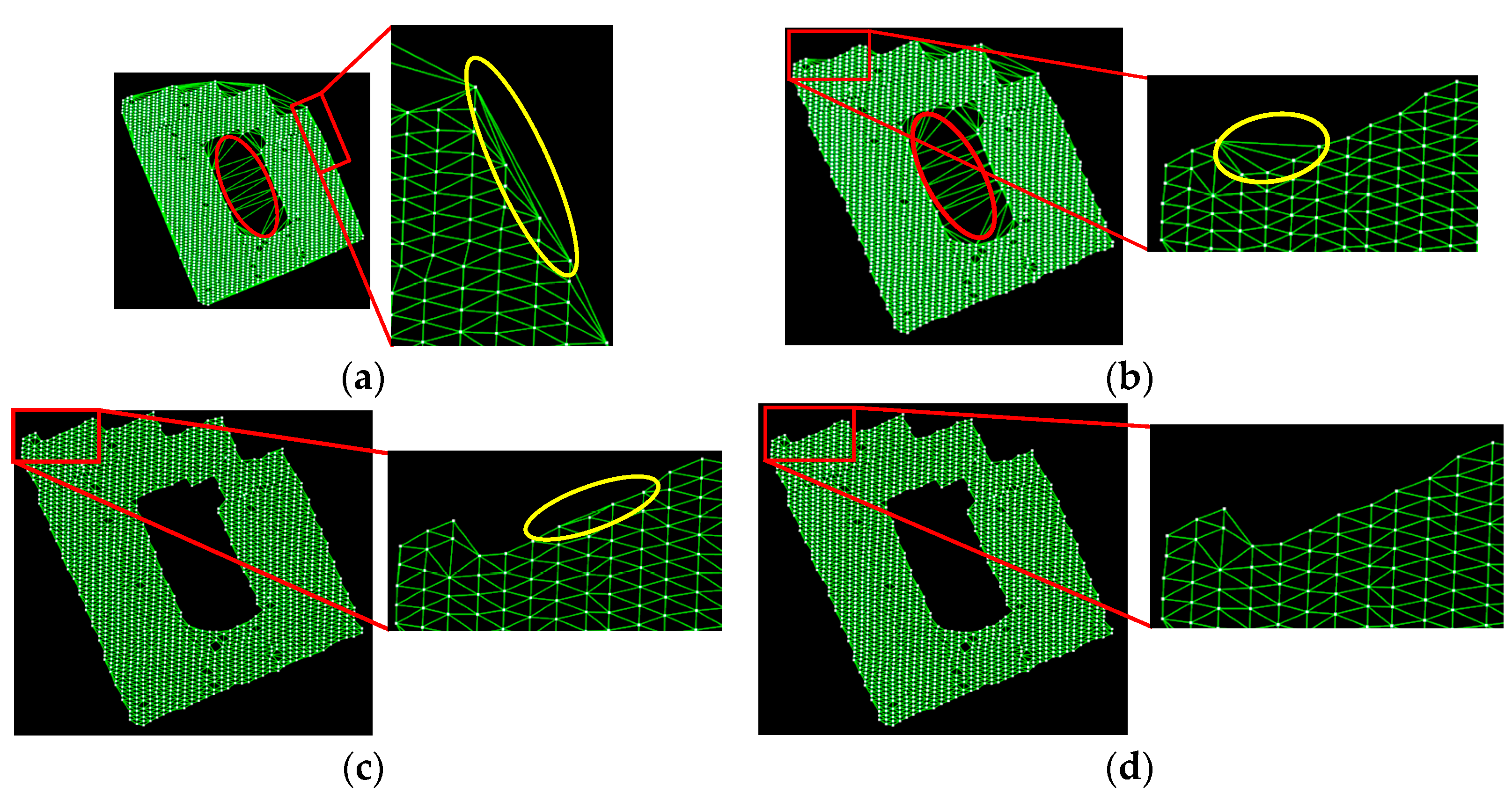
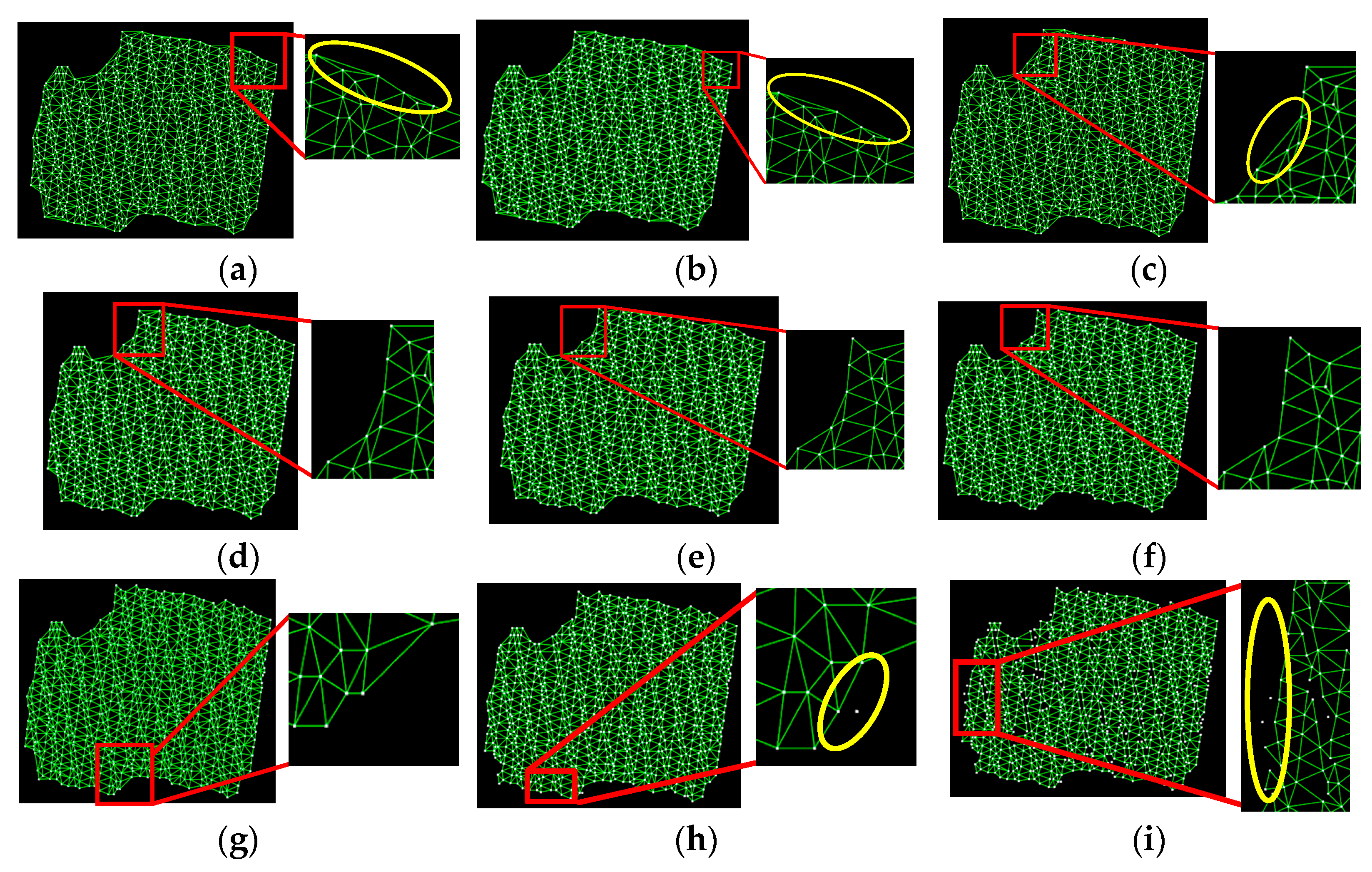
Figure 2a illustrates the constructed DT using the unorganized projected point clouds without any constraints, and it can be seen that many unnecessary triangles are generated (see the triangles in ellipses). These triangles cannot accurately describe the topological relationship between points and affect subsequent data processing. Therefore, the DT is optimized under the shape and side length constraints.

Let $a$, $b$, $c$ represent the lengths of three sides of a triangle, respectively. Its shape factor (SF) can be calculated as follows [48]:

$$SF={\displaystyle \frac{4\sqrt{3}A}{a^2+b^2+c^2}}$$

(2)

$$p={\displaystyle \frac{a+b+c}{2}}$$

(3)

$$A=\sqrt{p(p-a)(p-b)(p-c)}$$

(4)

The SF value ranges from 0 to 1.0, and the SF value of an equilateral triangle is 1.0. A large SF indicates small differences in the length of three sides, and such triangles are preferred during DT construction [48]. As shown in Figure 2a, the interior angles of the abnormal triangles in the yellow ellipse are either larger than or smaller than those of normal triangles. Therefore, if the SF value of a triangle is less than the threshold SF₀, then the triangle is removed. After the shape constraint, abnormal triangles are removed (see Figure 2b). The parameter SF₀ is related to the quality of the DT. Detailed discussions of the parameter SF₀ setting are in the Discussion Section.

However, many large triangles remain under shape constraint (see the triangle in the ellipse in Figure 2b). This is because the points that are far away from each other are used to construct triangles, and their shapes are normal. Thus, triangles are constrained by side length. Specifically, if the average side length S_ave of a triangle is larger than the predefined S₀, then the triangle is removed. Figure 2c illustrates the DT under the side length constraint, where large triangles are removed, but some abnormal triangles are still retained (see the ellipse in Figure 2c). Figure 2d illustrates the triangles under both shape and side length constraints. It can be observed that abnormal and large triangles are removed, and the constrained DT can accurately describe the shape of projected point clouds. According to [14], S₀ is set as twice the average point spacing.

3.1.2. Topology-Aware Loop Searching

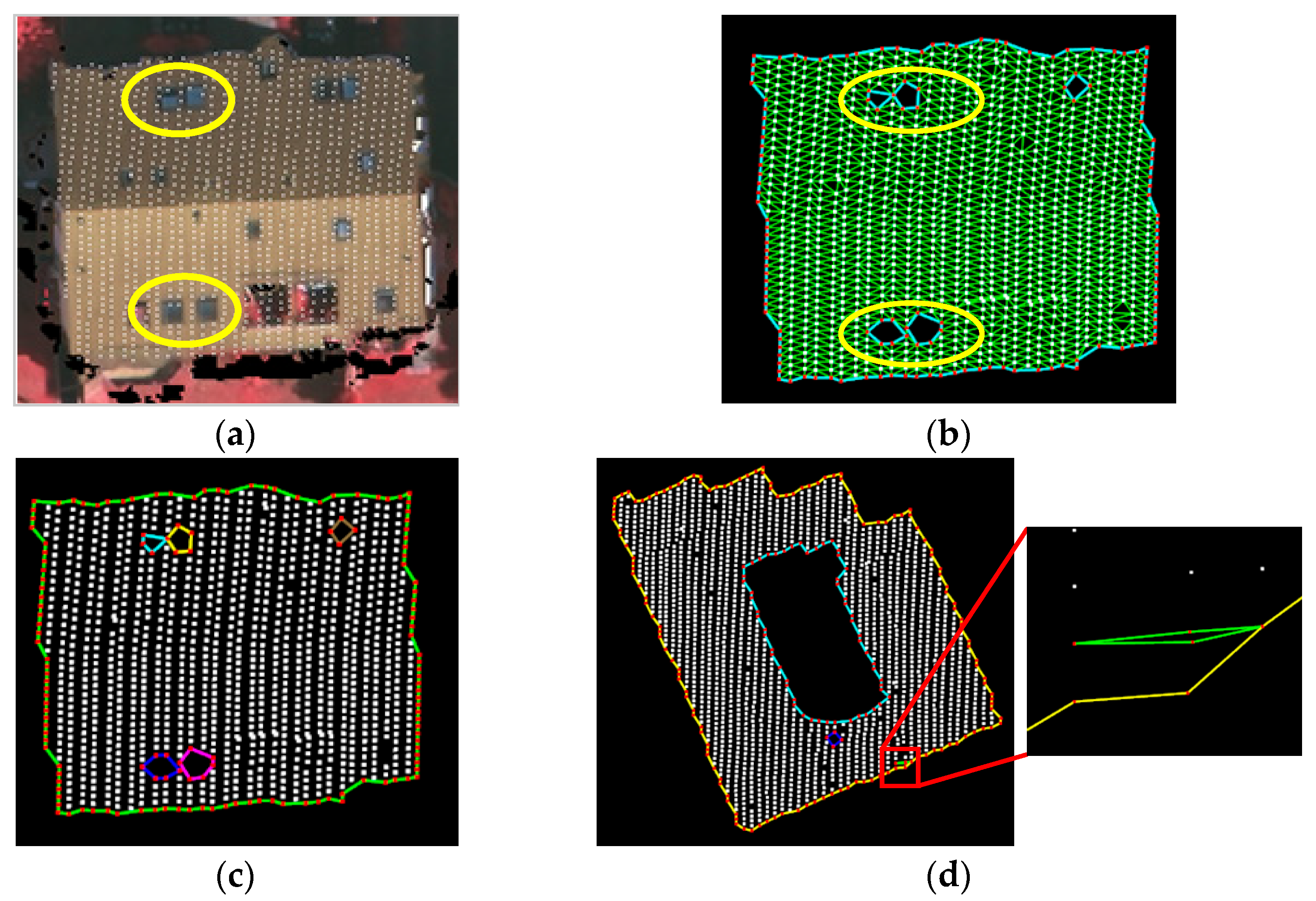
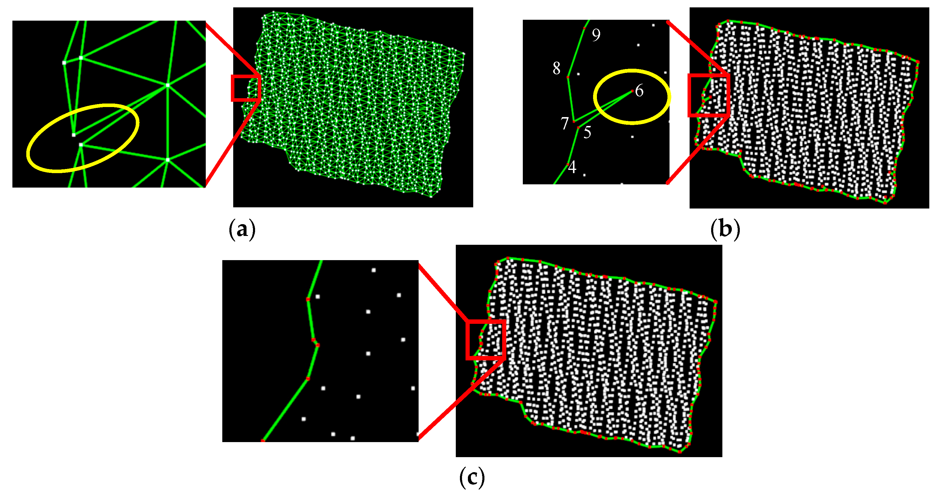
In Figure 3, triangles $T_1$ and $T_2$ are formed using points A, B, C, and D. Edges $S_{AB}$ and $S_{AC}$ belong only to the triangle $T_1$, while edge $S_{BC}$ belongs to both triangles $T_1$ and $T_2$. Based on this feature, edges that belong to only one triangle are defined as boundary edges, and corresponding points are defined as boundary points. Figure 3 shows the extracted boundary edges and boundary points, rendered in cyan and red, respectively. It can be seen that the extracted boundary points are satisfactory, with almost all boundary points successfully extracted.

However, some non-boundary points are incorrectly recognized as boundary points, see the ellipses in Figure 3 and Figure 4b. This is mainly due to two reasons. (1) Data missing. Possibly due to the roof material, some points are omitted and holes are formed (see the ellipses in Figure 4a). As a result, boundary points of the holes are incorrectly recognized as boundary points (see Figure 4b). (2) Uneven point density. In fact, the average point spacing of each point is different, but the thresholds used for DT construction are the same. In Figure 3, the distance between the two points in the red ellipse is very close. As a result, the triangle containing these two points is removed.

It should be noted that false boundary points can severely affect outline generation. However, for most existing methods, automatically recognizing false boundary points is a challenging task. Considering that building outlines are typically closed polygons composed of a finite number of ordered vertices [24,49]; therefore, we formulate the boundary point extraction as a topology-aware loop searching and parsing problem, which can preserve the sequence relationships and semantic information of boundary points. Although some researchers have employed the loop-based method for image edge detection with satisfactory results [50,51], the point clouds are scattered data, and existing image edge detection methods cannot be directly applied to them. Furthermore, these methods establish connections between pixels through nearest-neighbor pixel searches, which are not only susceptible to neighbor search parameters but also fail to consider the rationalization of these connections.

In the proposed method, loops are searched from the undirected graph, which is constructed using the initial boundary points and edges extracted based on the constrained DT. In the undirected graph G = (V, E), the initial boundary points form the vertices V, and the adjacency relationships between vertices are constructed according to the boundary edges. Specifically, if an edge is composed of boundary points p and q, then vertices p and q are adjacent. Because the constrained DT can accurately describe the projected point cloud shape, the connections between the vertices of graph G are reasonable. After constructing the graph, a depth-first search-based (DFS) [52] method is used to search for loops in a topologically aware manner. The pseudo-code is described in Algorithm 1.

Algorithm 1: Loop extraction

Notations:  Graph G = (V, E): An undirected graph with a set of vertices V and a set of edges E.  List C: A list of closed loops in graph G. Inputs: Graph G. Output: List C. Initialization:  Create an empty list C to store the searched closed loops.  For each vertex v∈V in the graph G, set its status to “Unvisited”. Begin:  for each vertex v in G   if v is “Unvisited”    Initialize an empty stack S.    Initialize an empty path list P to record the current path.    Mark v as “Visiting” and push it onto the stack S.    Add v to the path list P.   end if   while S is not empty:    Pop a vertex u from the top of S    for each adjacent vertex w of u     if w is “Visiting”      Record the sub-path SP from w to u in P.      Get the index min_index of the vertex with the minimum x in SP.      Get the sorted SP’ = SP[min_index: ] + SP[ : min_index].      Calculate area A(SP’) and geometric center GC(SP’) of SP’.      Set IsDuplicate = true.      for each loop in C       if A(SP’) ≠ A(loop) or GC(SP’) ≠ GC(loop)        IsDuplicate = false.        break.       else if vertices(SP’) ≠ vertices(loop)        IsDuplicate = false.        break.       end if      end for      if IsDuplicate = false       Add SP’ to C as a closed loop.       end if      else if w is “Unvisited”:      Mark w as “Visiting” and push it onto S.      Add w to P.     end if    end for    Mark u as “Visited”.    Remove u from the path list.   end while  end for Termination: The algorithm terminates when all vertices are marked as “Visited”.

In the loop extraction algorithm, for each extracted loop, a preliminary judgment is conducted based on its area and geometric center to determine whether it duplicates an existing loop. If uncertainty remains, vertex-by-vertex comparison is performed. Only non-duplicate loops are retained. Let $L=\{p_1\left(x_1,y_1,z_1\right),p_2\left(x_2,y_2,z_2\right),\dots ,p_n\left(x_n,y_n,z_n\right)\}$ denote the vertices of a closed loop. Its area A and geometric center $GC(x_{gc},y_{gc})$ are calculated as follows [24]:

$$\mathrm{A}={\displaystyle \frac{1}{2}}\left|\sum _{i=1}^n(x_i{y}_{i+1}-x_{i+1}{y}_i)\right|$$

(5)

$$x_{gc}={\displaystyle \frac{1}{n}}\sum _{i=1}^n{x}_i$$

(6)

$$y_{gc}={\displaystyle \frac{1}{n}}\sum _{i=1}^n{y}_i$$

(7)

Figure 4c,d illustrates the extracted loops by directly connecting boundary points of the loop, and edges belonging to the same loop are rendered in the same color. It can be seen that the loops accurately describe the shapes of holes and buildings, indicating that the sequence relationships between boundary points are correct. The reason is that the constrained DT can accurately construct topological relationships between points, and high-quality boundary points are extracted, which benefits subsequent loop extraction. Furthermore, during the loop extraction, the depth-first search (DFS) method records the visitation order of vertices along a path. When retracing a visiting vertex, the algorithm extracts the sub-path between these two vertices from the path record, thus forming a loop.

3.1.3. Semantic Boundary Point Extraction

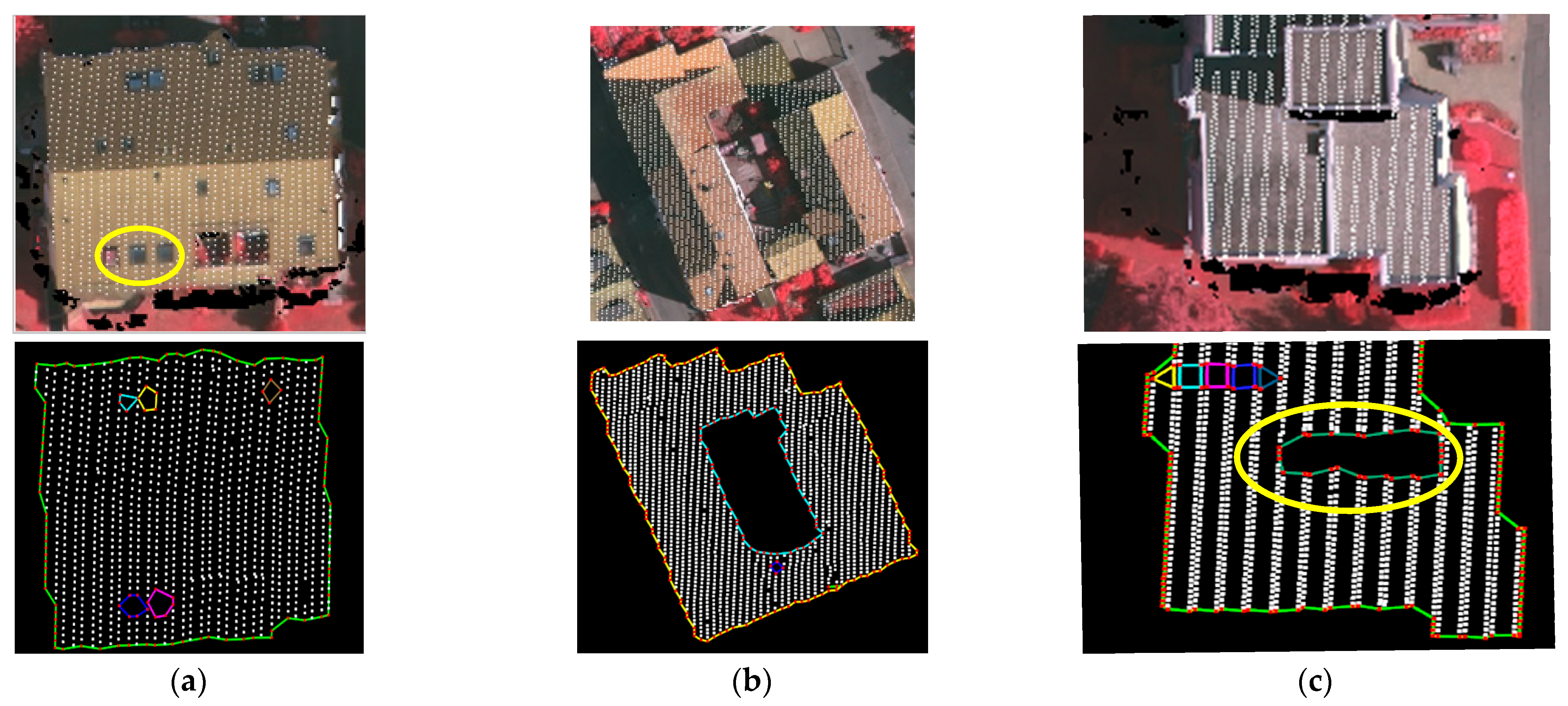
In Figure 5, the outermost loops can accurately describe the shape of projected point clouds. Therefore, in the proposed method, points of the loop with the maximum area are defined as outer boundary points. In addition to the outer loop, loops of holes and courtyards are also extracted (see Figure 5a,c). Generally, the sizes of holes are relatively small. Therefore, area-based strategies are commonly used to recognize hole boundary points [4,15]. Specifically, boundary points of the loops with areas smaller than the threshold are defined as hole boundary points. As shown in the ellipse in Figure 5c, a large hole is formed due to data missing. The area of the hole is about 18 m², so the area threshold should be larger than 18 m². However, in practice, areas of many courtyards are smaller than 18 m².

To address the issue, the minimum bounding rectangle (MBR) is used to depict the shape of loops. For a loop, a dominant direction is determined using any two adjacent boundary points. A rectangle that is parallel or perpendicular to the dominant direction and contains all boundary points is calculated. Among all these rectangles, the one with the maximum number of boundary points within a normal-distance threshold is selected as the MBR of the loop. For more details, please refer to [41].

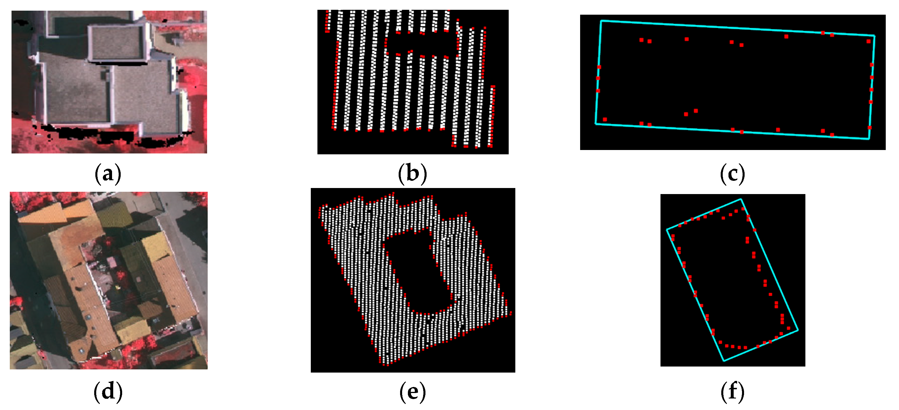
Figure 6c,f illustrate the MBR of the hole and courtyard boundary points. It can be seen that the MBR can accurately describe the overall shape of the boundary points. According to [53,54], courtyards are used for human activities, and the rectangle ratio R of rectangular courtyards is about 2:1 to 3:1, and rectangular courtyards with a width W exceeding 3 m are considered reasonable.

Considering circular and triangular courtyards, points G of a loop are classified into three categories (i.e., outer, courtyard, and hole boundary points) as follows:

$$G=\left\{\begin{array}{cc}\mathrm{o}\mathrm{u}\mathrm{t}\mathrm{e}\mathrm{r}& \mathrm{w}\mathrm{i}\mathrm{t}\mathrm{h} \mathrm{t}\mathrm{h}\mathrm{e} \mathrm{m}\mathrm{a}\mathrm{x}\mathrm{i}\mathrm{m}\mathrm{u}\mathrm{m} \mathrm{a}\mathrm{r}\mathrm{e}\mathrm{a}\\ \mathrm{c}\mathrm{o}\mathrm{u}\mathrm{r}\mathrm{t}\mathrm{y}\mathrm{a}\mathrm{r}\mathrm{d}& if \left(1.0\le R\le 3.0\right)\cap (W\ge 3.0)\\ \mathrm{h}\mathrm{o}\mathrm{l}\mathrm{e}& \mathrm{o}\mathrm{t}\mathrm{h}\mathrm{e}\mathrm{r}\mathrm{w}\mathrm{i}\mathrm{s}\mathrm{e}\end{array}\right.$$

(8)

The length and width of the MBR of the boundary points in Figure 6c are 2.7 m × 7.5 m, and the length and width in Figure 6f are 9.6 m × 17.0 m. According to the above rules, boundary points in Figure 6c,f are identified as hole boundary points and courtyard boundary points, respectively. Boundary points of courtyards are preserved, while those of holes are defined as non-boundary points.

Although satisfactory boundary points can be obtained in most cases, some boundary points are still incorrectly extracted due to the uneven point distribution. In Figure 7a, the distance between two points inside the ellipse is very close, and the triangle containing these two points is removed. As a result, incorrect boundary points are extracted (see points in the ellipse in Figure 7b).

To remove these false boundary points, a strategy based on neighborhood sequence analysis is proposed. Let $NP=\{p_1,\dots ,p_i,\dots ,p_n\}$ denote the sequential boundary points. For each point $p$, search for the nearest neighborhood $q$ in $NP$. If the index of a point lies between $p$ and $q$, then the point is defined as the false boundary point. In Figure 6b, for point 5, its nearest neighborhood is point 7. Point 6 is located between points 5 and 7. Therefore, point 6 is identified as a non-boundary point (see Figure 7c).

3.2. Outline Regularization

3.2.1. Dominant Direction and Line Segment Extraction

In general, building outlines are composed of multiple line segments, most of which are parallel or perpendicular to the dominant directions. Since the angle analysis-based method [24] can reduce the influence of LiDAR scanning direction on the dominant direction detection; therefore, this method is used to estimate dominant directions. The method groups boundary points using the iterative region growing (IRG) algorithm, and then the angular standard deviation is used to select group boundary points to calculate building dominant directions.

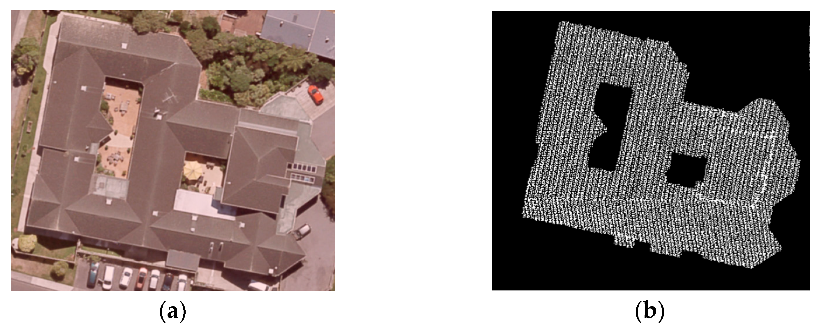
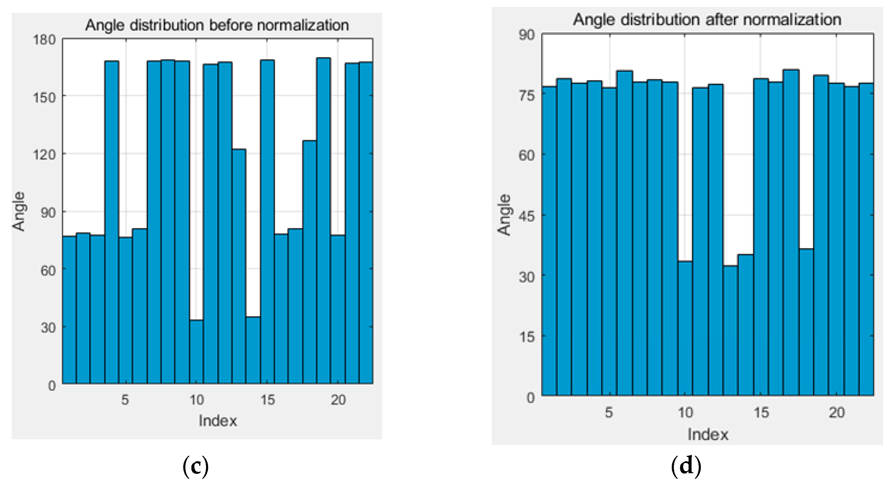
For a complex building (see its image and projected point clouds in Figure 8a,b), 22 dominant directions are detected from outer boundary points, and Figure 8c shows the anticlockwise angles between the dominant directions and the x-axis. It can be observed that the differences between some angles are minimal, while others are close to 90$°$. This indicates that these detected dominant directions are approximately parallel or perpendicular. If all dominant directions are used for regularization, line segments that should be strictly parallel or perpendicular will exhibit slight angular deviations, and the regularized outline fails to accurately depict the shape of projected point clouds.

Most existing methods simply merge initial dominant directions according to the angles between them, failing to fully utilize the potential parallel and perpendicular relationships between them [24,55,56,57], resulting in inaccurate dominant directions. To address the issue, a method based on angle normalization, merging, and perpendicular pairing is proposed, which fully exploits the potential parallel and perpendicular relationship between dominant directions, as well as the weights of different dominant directions. The method includes the following sub-steps.

Step 1: For each initial dominant direction, calculate its counterclockwise angle $\alpha$ relative to the x-axis and normalize $\alpha$ to the range [0$°$, 90$°$) as follows:

$$\alpha =\left\{\begin{array}{cc}\alpha & 0°\le \alpha <90°\\ \alpha -90°& \alpha \ge 90°\end{array}\right.$$

(9)

Step 2: Sort the normalized angles in ascending order and calculate the angular difference $\delta$ between adjacent normalized angles. If the minimum angular difference ${\delta }_{min}$ is less than the threshold ${\delta }_0$, then merge adjacent ${\alpha }_i$ and ${\alpha }_j$ as follows:

$$\overline{\alpha }={\displaystyle \frac{n_i{\alpha }_i+n_j{\alpha }_j}{n_i+n_j}}$$

(10)

where $n_i$ and $n_j$ represent the number of boundary points corresponding to the dominant directions of angles ${\alpha }_i$ and ${\alpha }_j$, respectively. $\overline{\alpha }$ is the merged angle, replacing ${\alpha }_i$ and ${\alpha }_j$. For $\overline{\alpha }$, the number of boundary points is $n_i+n_j$.

Step 3: Repeat Step 2 until ${\delta }_{min}$ exceeds ${\delta }_0$.

Step 4: Calculate the angular difference $\delta$ between the maximum angle ${\alpha }_{max}$ and the minimum angles ${\alpha }_{min}$ as follows:

$$\delta =\left|90°-{\alpha }_{max}+{\alpha }_{min}\right|$$

(11)

If $\delta$ is larger than ${\delta }_0$, then go to Steps 5 and 6. Otherwise, stop.

Step 5: Let $n_{max}$ and $n_{min}$ denote the number of boundary points corresponding to the dominant directions of angles ${\alpha }_{max}$ and ${\alpha }_{min}$. If $n_{max}\ge n_{min}$, then the merged angle $\overline{\alpha }$ is calculated as follows:

$${\alpha }_{min}={\alpha }_{min}+90°$$

(12)

$$\overline{\alpha }={\displaystyle \frac{n_{max}{\alpha }_{max}+n_{min}{\alpha }_{min}}{n_{max}+n_{min}}}$$

(13)

If $n_{max}<n_{min}$, then the merged angle $\overline{\alpha }$ is calculated as follows:

$$n_{max}=90°-n_{max}$$

(14)

$$\overline{\alpha }={\displaystyle \frac{n_{max}{\alpha }_{max}+n_{min}{\alpha }_{min}}{n_{max}+n_{min}}}$$

(15)

Step 6: All angles are normalized to the range [0$°$, 90$°$).

In practice, line segments of building outlines are always parallel or perpendicular. Thus, the merged angles are perpendicularly paired. Specifically, the paired angle of ${\alpha }_i$ is ${\alpha }_i+90°$. After pairing, each angle represents a dominant direction.

By merging the normalized angles, we obtain 34.37° and 78.02° (see Figure 8d). Thus, four dominant directions are obtained after perpendicular pairing, corresponding to angles 34.37°, 124.37°, 78.02°, and 168.02°. The process of merging dominant directions involves an angle threshold ${\delta }_0$. For a detailed discussion on the parameter δ₀ setting, see the Discussion Section.

Line segments of outlines are obtained using the hierarchical merging method [24]. In this method, over-segment line segments are first extracted via the IRG algorithm. Then these over-segmented line segments are merged in a bottom-to-top manner under the constraints of angular difference and point-to-line distance. For more details, please refer to [24].

3.2.2. Parallel Constraint-Based Outline Regularization

Since all dominant directions are accurately extracted and perpendicularly paired, and the number of dominant directions is not limited; therefore, in the proposed method, each line segment is strictly parallel to the optimal dominant direction. For most existing methods [13,40], the optimal dominant direction is selected based solely on the angle between the line segments and the dominant direction. However, the angle-based criterion does not consider line segment length and boundary point distribution. In addition, it is not friendly to short line segments because they are more susceptible to noise than long line segments.

Therefore, a parallel constraint-based method is proposed to regularize outlines, which includes the following steps.

Step 1: For a line segment and its boundary points $NP=\left\{p_1\right(x_1,y_1,z_1),\dots ,p_i(x_i,y_i,z_i),\dots ,p_n(x_n,y_n,z_n\left)\right\}$, $\alpha =\{{\alpha }_1,\dots ,{\alpha }_i,\dots {\alpha }_n\}$ denotes the angles of dominant directions, calculate the linear equation $y=kx+b$ and unit length residual $\sigma$ using the angle ${\alpha }_i$ and boundary points NP via the least-square fitting technique, as follows [55]:

$$k=\mathrm{t}\mathrm{a}\mathrm{n}\left({\alpha }_i\right)$$

(16)

$$b={\displaystyle \frac{1}{n}}\sum _{i=1}^n(y_i-k{x}_i)$$

(17)

$$\epsilon =\sqrt{\sum _{i=1}^n{\displaystyle \frac{{(k{x}_i+b-y_i)}^2}{1+k^2}}}$$

(18)

$$\sigma ={\displaystyle \frac{\epsilon }{L}}$$

(19)

where $\mathrm{t}\mathrm{a}\mathrm{n}(·)$ is the tangent function, $\epsilon$ is the fitting error between the boundary points and the fitted line, $L$ is the length of the line segment.

Step 2: Select the linear equation ($y=k_{opt}x+b_{opt}$) with the minimum $\sigma$ as the linear equation for the line segment, and project all boundary points onto the line as follows [58]:

$$x_{proj}={\displaystyle \frac{x_i+k_{opt}(y_i-b_{opt})}{1+k_{opt}^2}}$$

(20)

$$y_{proj}={\displaystyle \frac{k_{opt}\left(x_i+k_{opt}{y}_i\right)+b_{opt}}{1+k_{opt}^2}}$$

(21)

where $(x_{proj}, y_{proj})$ are the coordinates of the projected points.

Step 3: Repeat Steps 1 and 2 for other line segments.

Each line segment is adjusted to be parallel to the optimal dominant direction according to the unit length residual $\sigma$. Based on the above description, parameter $\sigma$ considers the fitting error $\epsilon$ between boundary points and the fitted line, ensuring that the adjusted line segments align with the projected point clouds. This eliminates situations where the angle between the optimal direction and the line segment to be adjusted is small, but boundary points remain misaligned. In addition, the impact of length on fitting error is reduced by using the ratio of ε to L, thereby minimizing noise effects on short line segments.

After adjusting line segments, the corners between adjacent non-parallel line segments are calculated via line intersection. If two adjacent line segments are parallel, then a perpendicular line segment is inserted, and the inserted line passes through the midpoint of the two endpoints of the adjacent adjusted line segments.

4. Experiment and Analysis

Datasets in Vaihingen, Germany, provided by the International Society for Photogrammetry and Remote Sensing (ISPRS) (https://www2.isprs.org/commissions/) (accessed on 28 August 2025) and New Zealand (https://portal.opentopography.org/lidarDataset?opentopoID=OTLAS.092020.2193.1) (accessed on 28 August 2025) were used to validate the proposed method. All experiments were conducted on a laptop computer with 16 GB RAM and an Intel Core i7-12700H @2.4 GHz processor. The equipment was sourced from Lenovo, located in Wuhan, China.

4.1. Data Description

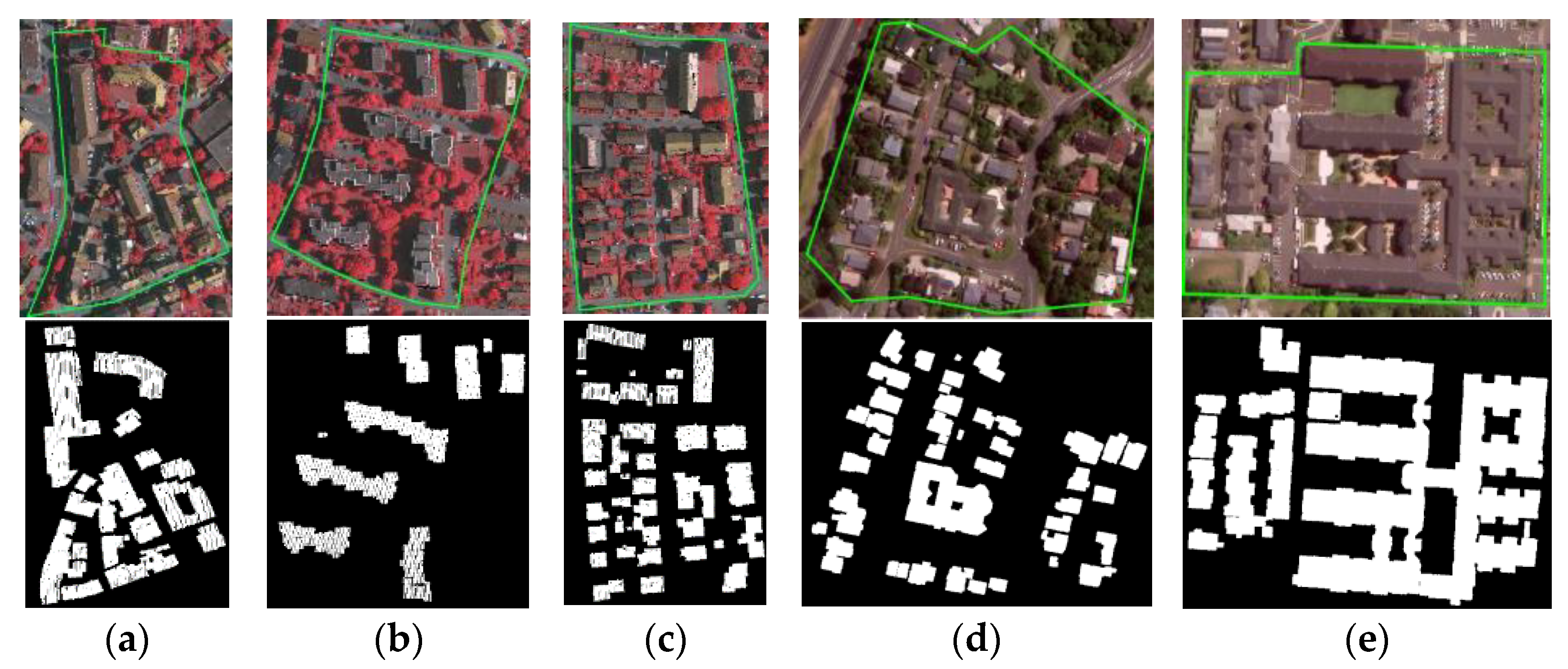
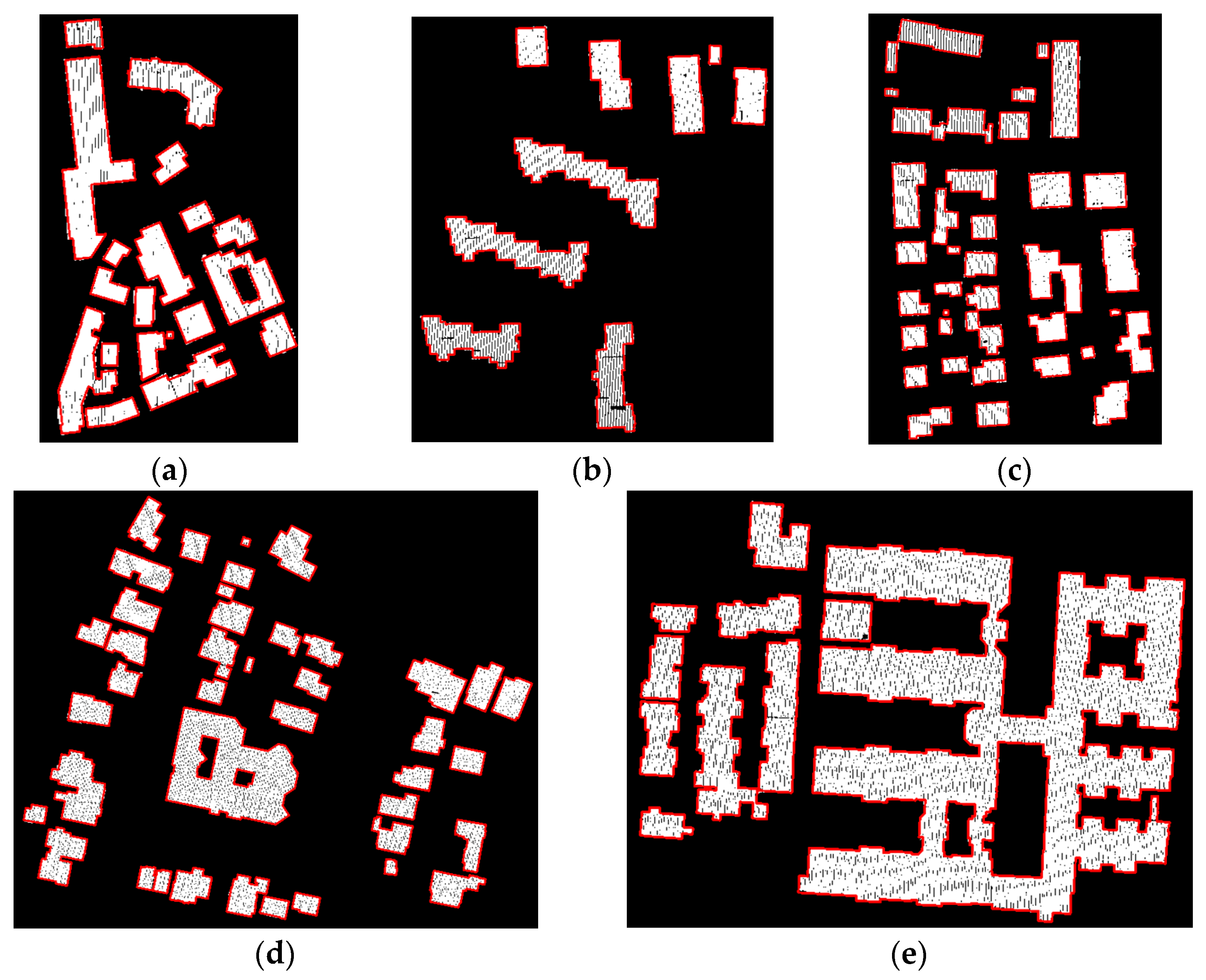
Vaihingen includes three test areas: Areas 1 to 3, while New Zealand consists of two test areas: Areas 4 to 5. The average point density in Vaihingen is about 4.0 points/m², while the average point density in New Zealand is approximately 23.3 points/m². It should be noted that Areas 1 to 3 are located within residential areas and include a building with courtyards. Whereas, in Areas 4 and 5, two large buildings contain multiple courtyards. In addition, projected point clouds in New Zealand are more scattered than those in Vaihingen, increasing the difficulty of extracting boundary points and outlines. The distribution and shape of buildings are shown in Figure 9.

4.2. Boundary Point Extraction

Figure 10 illustrates the boundary point extraction results of the proposed method. Outer boundary points are rendered in red, while boundary points of the same courtyard are rendered in other colors. Non-boundary points are rendered in white. It can be seen that boundary points of buildings with one, two, and three courtyards are all successfully extracted (see the rectangles in Figure 10a,d,e). The satisfactory results benefit outline generation.

Four state-of-the-art methods: the maximum angle method (MA) [16], the Alpha Shapes method (AS) [59], the Adaptive Tracing Alpha Shapes method (ATAS) [24], and the Triangulation-based method (TB) [13] were selected for comparison with the proposed method. Buildings A to F were selected for visual comparisons, and the comparison results are shown in Figure 11. It should be noted that the green rectangles denote the erroneous boundary points and the blue rectangles represent the omitted boundary points.

For Building A, all methods successfully extract boundary points. However, only the proposed method and the ATAS methods can distinguish between outer and courtyard boundary points. Additionally, except for the proposed and ATAS methods, the boundary points extracted by the other methods are nonsequential. For Building B, a large hole is formed due to data missing. As a result, except for the proposed and ATAS methods, the TB, AS, and MA methods extract false boundary points, see the rectangles. Because the ATAS method does not recognize the hole, the boundary points of the hole are not extracted. For the proposed method, hole boundary points are recognized based on the semantic rules on the MBR (see Figure 6). For Building C, the TB and MA methods extract false boundary points due to uneven point density and unreasonable parameter settings, see the rectangles. In addition, some boundary points are obviously omitted by the TB method, see the arrows. This is because the constructed Delaunay triangulation in the TB method cannot accurately construct the topological relationship between points, see the ellipse. Buildings D and E contain two and three courtyards, respectively. Only the proposed method successfully extracts boundary points. This is because the constrained Delaunay triangulation can accurately describe the shape of projected point clouds, and the proposed method can identify false boundary points by parsing geometric characteristics of the loops formed by these boundary points. TB, AS, and MA methods extract false boundary points due to uneven point density and data missing, see the rectangles. For the ATAS method, only the boundary points of a single courtyard can be extracted. This is because the ATAS method only considers buildings that have at most one courtyard. For Buildings F, due to the uneven point density, the TB and MA methods extract false boundary points, see the rectangles, while the other three methods all successfully extract boundary points.

In addition to visual comparisons, four precision metrics are selected for the qualitative assessment: completeness CP%, correctness CR%, quality Q%, and F₁-score F₁%. Completeness represents the percentage of correctly extracted boundary points to the total number of reference boundary points. Correctness denotes the percentage of correctly extracted boundary points to the total number of extracted boundary points. Quality and $F_1$-score provide a compound performance metric that balances completeness and correctness. Relevant formulas are as follows [60,61]:

$$\begin{array}{c}\begin{array}{c}\mathrm{C}\mathrm{P}={\displaystyle \frac{\left|\mathrm{T}\mathrm{P}\right|}{\left|\mathrm{T}\mathrm{P}\right|+\left|\mathrm{F}\mathrm{N}\right|}}\\ \mathrm{C}\mathrm{R}={\displaystyle \frac{\left|\mathrm{T}\mathrm{P}\right|}{\left|\mathrm{T}\mathrm{P}\right|+\left|\mathrm{F}\mathrm{P}\right|}}\end{array}\\ \begin{array}{c}\mathrm{Q}={\displaystyle \frac{\left|\mathrm{T}\mathrm{P}\right|}{\left|\mathrm{T}\mathrm{P}\right|+\left|\mathrm{F}\mathrm{N}\right|+\left|\mathrm{F}\mathrm{P}\right|}}\\ {\mathrm{F}}_1={\displaystyle \frac{2\ast \mathrm{C}\mathrm{P}\ast \mathrm{C}\mathrm{R}}{\mathrm{C}\mathrm{P}+\mathrm{C}\mathrm{R}}}\end{array}\end{array}$$

(22)

where $\left|\mathrm{T}\mathrm{P}\right|$ is the number of correctly extracted boundary points, $\left|\mathrm{F}\mathrm{N}\right|$ corresponds to the number of omitted boundary points, and $\left|\mathrm{F}\mathrm{P}\right|$ denotes the number of incorrectly extracted boundary points.

In addition, the running time is also discussed. The proposed method was implemented using C++ 14 with the platform of Visual Studio 2019. It should be noted that the total time (T) of boundary point extraction consists of two parts: time (T₁) of DT construction and optimization and time (T₂) of loop detection and parsing. Moreover, the memory RAM usage in DT construction and optimization is also evaluated.

Table 1. Quantitative evaluation of the proposed method.

	Vaihingen				New Zealand
	Area 1	Area 2	Area 3	Average	Area 4	Area 5	Average
Number of points	21,775	17,370	26,892	22,012	139,566	221,279	180,422
CP%	98.26	93.11	94.29	95.22	94.38	94.41	94.40
CR%	99.75	99.65	97.88	99.09	97.95	98.52	98.24
Q%	98.01	92.80	92.40	94.40	92.56	93.09	92.83
F1%	99.00	96.27	96.05	97.11	96.13	96.42	96.28
T1(s)	0.40	0.30	0.48	0.39	2.74	7.51	5.13
T2(s)	0.04	0.04	0.07	0.05	1.14	2.17	1.65
T(s)	0.44	0.34	0.55	0.44	3.88	9.68	6.78
RAM (MB)	2.98	2.78	3.33	3.03	19.66	31.68	25.67

lists the evaluation results of the proposed method. It can be seen that the minimum values of the CR metric are 97.88% and 97.95% in Vaihingen and New Zealand, respectively, indicating that the extracted boundary points are almost real boundary points, which benefits outline generation. Furthermore, the differences in the Q and F₁ metric values are minimal, which demonstrates the stability of the proposed method. This can be explained by two reasons: (1) The constrained Delaunay triangulation (DT) can accurately construct correct topological relationships between scattered points and depict the shape of projected point clouds, which benefits boundary point extraction. (2) False boundary points, caused by uneven point density, unreasonable parameter settings, and complex building structures, can be recognized by searching and parsing loops formed by these false boundary points. When the number of points in Area 4 is approximately 140,000, the running time is approximately 4s, and the efficiency is satisfactory. In addition, the proportion of time spent on DT construction and optimization in Vaihingen is remarkably higher than in New Zealand. This is because projected point clouds in New Zealand are more scattered and of higher density than Vaihingen, leading to more points being wrongly identified as boundary points. The loop extraction method based on depth-first search (DFS) is $O(V+E)$ [62], where V represents the number of vertices and E is the number of edges. Thus, loop searching and parsing take a longer time in New Zealand. A feasible solution is to employ CUDA or parallel computing techniques to accelerate loop searching.

Memory consumption (RAM) for DT construction and optimization increases approximately linearly with the number of input point clouds (see Table 1). More than 220,000 points consume 31.68 MB of memory for DT construction and optimization, validating the proposed method’s potential capability to process large-scale point clouds.

Table 2. Average evaluation results comparison of boundary point extraction. (The best values in each column are shown in bold).

	Vaihingen					New Zealand
	CP%	CR%	Q%	F1%	T(s)	CP%	CR%	Q%	F1%	T(s)
Proposed	95.22	99.09	94.40	97.11	0.44	94.40	98.24	92.83	96.28	6.78
TB	74.53	96.70	72.68	84.06	0.38	84.73	98.01	83.30	90.86	6.01
AS	97.23	94.35	91.84	95.74	1.47	86.37	98.72	85.41	92.13	21.21
ATAS	97.69	93.88	91.78	95.71	0.68	84.73	98.01	83.30	90.89	4.33
MA	96.48	92.89	89.78	94.61	0.22	94.24	92.78	87.79	93.50	1.93

lists the quantitative comparison results. It can be seen that the proposed method has the highest Q and F₁ metric values. In New Zealand, the Q and F₁ metrics of the proposed method are 92.83% and 96.28%, which are significantly better than the other methods. Both the TB and the proposed methods are based on triangulation to extract boundary points, but the differences in CP, Q, and F₁ metrics between them are large. This is because the triangulations constructed in the TB method cannot accurately describe the topological relationships between points, leading to both missed and erroneous extraction of boundary points. For the proposed method, erroneous boundary points are identified through parsing geometric characteristics of the loops formed by these boundary points. Accuracy differences between the AS and ATAS methods in New Zealand are larger than those in Vaihingen. This is because the projected point clouds in New Zealand are more scattered, and many buildings contain courtyards.

In terms of efficiency, the MA method has the shortest running time due to its simple judgment criteria. However, its extracted boundary points are nonsequential. For the proposed method, it is slightly lower than the TB method. This is because, in addition to the triangulation construction and optimization, the proposed method also searches and parses loops from the undirected graph to extract accurate semantic boundary points. The AS method has the longest running time among all methods. The ATAS is superior to the AS because partial points involve boundary point extraction.

4.3. Outline Extraction

Figure 12 illustrates the outline extraction results. It can be seen that the proposed method can successfully extract outer and courtyard outlines, and the outlines are aligned with projected point clouds. In addition, the extracted outlines are attractive, and most line segments are parallel or perpendicular to each other, which is consistent with the actual shape of buildings. This can be explained by two main reasons: (1) Dominant directions are accurate and reliable, and all dominant directions are perpendicularly paired, which ensures the parallel and perpendicular relationships between line segments after regularization. (2) During the regularization process, both the fitness between the dominant direction and boundary points and the length of line segments are considered, ensuring that the regularized outlines align with the projected point clouds.

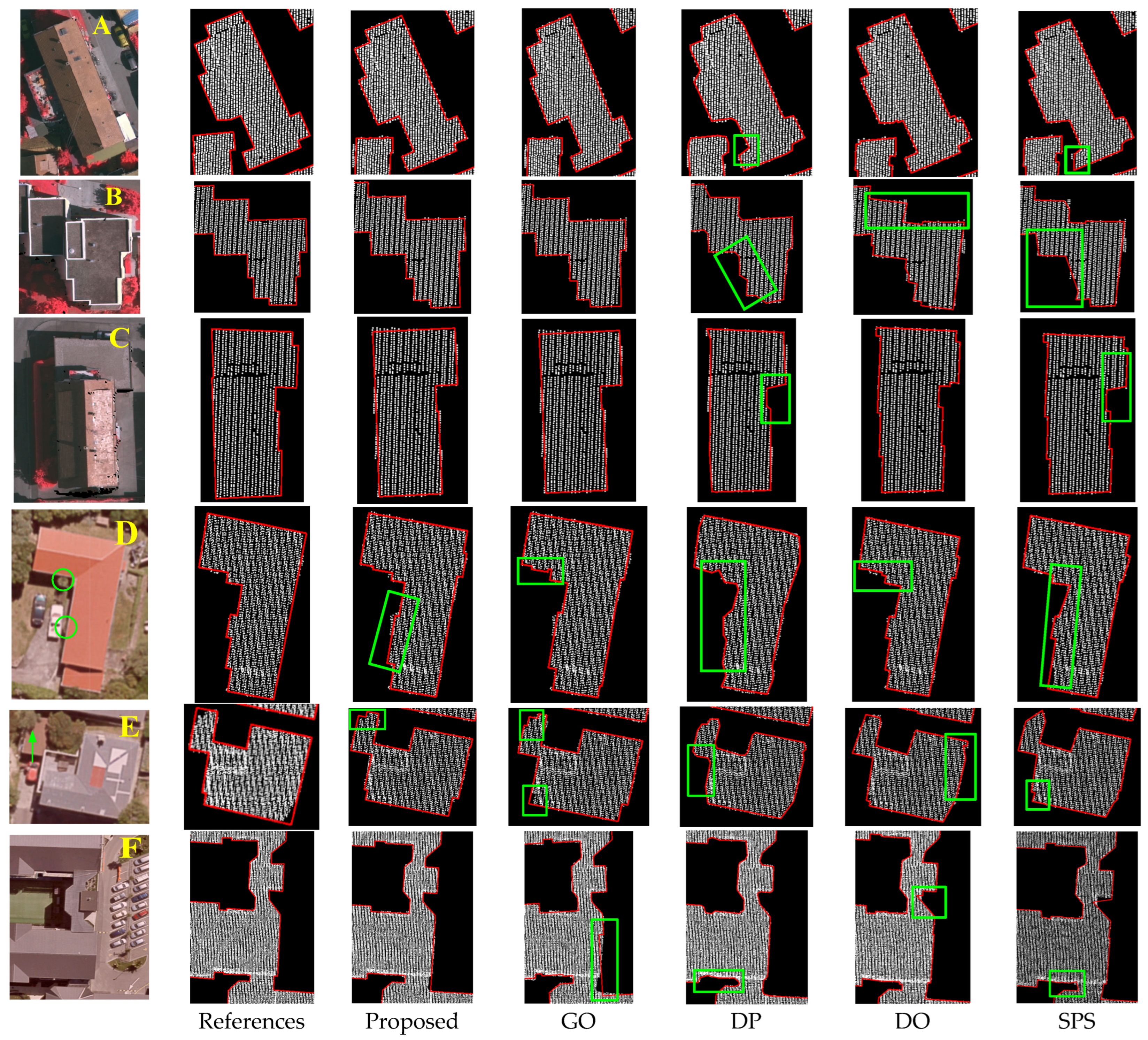
Four state-of-the-art methods—the Douglas-Peucker method (DP) [34], sleeve-fitting polyline simplification method (SPS) [63], dominant direction method (DO) [40], and global optimization method (GO) [24]—were selected for comparison with the proposed method. Figure 13 shows the visual comparison results. Buildings A to C are selected from Vaihingen, while Buildings D to F are selected from New Zealand. For the DP and SPS methods, the extracted outlines are jagged, and most line segments are neither parallel nor perpendicular, see the rectangles, which is neither attractive nor consistent with the real shapes of buildings. This is because these two methods only simplify boundary points without considering the potential parallel and perpendicular geometric relationships between line segments.

For the DO method, the extracted outlines are relatively attractive compared with the DP and SPS methods. Specifically, for buildings with simple shapes (e.g., Buildings A and C in Figure 13), the extracted outlines are satisfactory, and most of the line segments are parallel or perpendicular. However, for complex buildings (e.g., Buildings B, D, E, and F), the extracted outlines cannot accurately depict the building shapes (see the rectangles). This can be attributed to two reasons. (1) Inaccurate dominant direction. In the DO method, the dominant directions are estimated based solely on the longest line segment, which is susceptible to noise. (2) Scattered projected point clouds. Each line segment is adjusted based on the angle between it and the dominant direction, which is sensitive to noise and does not consider boundary point distribution. As a result, adjusted line segments cannot accurately align with projected point clouds.

Compared with other methods, the proposed and GO methods extract attractive outlines that conform to human vision cognition (e.g., Buildings A, B, and C). However, outlines of Buildings D and E are not satisfactory compared with the proposed method, see the rectangles. It should be noted that these two methods can extract outlines of buildings with more than two non-perpendicular dominant directions, see Buildings F. Building F is a very large building composed of multiple small buildings, and its length and width are approximately 133 m * 131 m, respectively. Outlines extracted by the GO method do not align with the projected point clouds of Building F (see the rectangles). This is because the dominant directions are inaccurate, and line segments are adjusted according to the extracted dominant directions in the GO method. In contrast, the proposed method can extract accurate dominant directions, and satisfactory outlines are obtained. However, some building outlines cannot be perfectly extracted by the proposed method. Two reasons can be explained: (1) Partial points near the building boundaries are omitted due to occlusion (see the arrow in the image of Building E). Because the proposed method extracts outlines solely based on point cloud data. Therefore, the extracted outlines cannot accurately describe real building shapes, see the rectangle. A possible solution to the issue is to fuse LiDAR data and images. (2) Irregular objects attach to the building boundaries (see the circles in Building D image), and their outlines are neither parallel nor perpendicular to the dominant directions. As a result, the extracted outlines fail to align with the projected point clouds.

Two different evaluation metrics: corner geometric accuracy and shape accuracy, are selected to quantitatively evaluate the extracted outlines. Corner accuracy is evaluated using root mean square error (RMSE), calculated as follows [64]:

$$\begin{array}{c}{RMSE}_X=\sqrt{{\displaystyle \frac{\sum {(X_{ext}-X_{ref})}^2}{n}}}\\ {RMSE}_Y=\sqrt{{\displaystyle \frac{\sum {(Y_{ext}-Y_{ref})}^2}{n}}}\\ \mathrm{R}\mathrm{M}\mathrm{S}\mathrm{E}=\sqrt{{{RMSE}_X}^2+{{RMSE}_Y}^2}\end{array}$$

(23)

where $(X_{ext},Y_{ext})$ and $(X_{ref},Y_{ref})$ represent the coordinates of the extracted corners and reference corners, respectively. $n$ denotes the number of extracted corners within a 3 m radius around the corresponding reference corners [24,65].

Shape accuracy of the extracted outlines is evaluated using the PoLiS metric $p(A,B)$, defined as follows [66]:

$$p\left(A,B\right)={\displaystyle \frac{1}{2q}}\sum _{a_i\in A}{}_{b\in \partial B}{}^{min}\left|a_i-b\right|+{\displaystyle \frac{1}{2r}}\sum _{b_j\in B}{}_{a\in \partial A}{}^{min}\left|b_j-a\right|$$

(24)

where $q$ and $r$ represent the number of vertices of polygons A and B, respectively. $\partial A$ and $\partial B$ are the vertices of polygons A and B, respectively. $|a-b|$ denotes the Euclidean distance between points $a$ and $b$.

Furthermore, the robust corner correspondence (RCC) metric is selected to evaluate the overall dissimilarity between the regularized outlines and the reference outlines, described as follows [67]:

$$d_{avg}\left(S_e,S_r\right)={\displaystyle \frac{1}{n}}\sum _{i=1}^n{d}_p$$

(25)

where $S_e$ and $S_r$ are the extracted and reference outlines, respectively, n is the number of extracted outline vertices $S_e$, and $d_p$ is the perpendicular distance from a vertex of $S_e$ to the corresponding reference line of $S_r$.

Table 3. Shape accuracy of the outline extracted by the proposed method in Areas 1 to 5.

Dataset		RMSE	PoLiS	RCC	T (s)
Vaihingen	Area 1	0.87	0.84	0.69	0.89
	Area 2	0.68	0.60	0.57	0.58
	Area 3	0.90	0.68	0.65	1.41
New Zealand	Area 4	0.78	0.49	0.51	3.24
	Area 5	0.94	0.60	0.62	3.34

lists the shape accuracy and running time T of the outlines extracted by the proposed method, and

Table 4. Average evaluation results comparison of outline extraction (the best values per column are shown in bold font).

Methods	Vaihingen				New Zealand
	RMSE	PoLiS	RCC	T(s)	RMSE	PoLiS	RCC	T (s)
Proposed	0.81	0.71	0.64	0.96	0.86	0.55	0.56	3.29
GO	0.82	0.70	0.63	0.92	0.96	0.61	0.66	2.64
DO	1.17	0.87	0.92	0.38	0.89	0.58	0.59	1.02
DP	0.89	0.78	0.73	0.01	0.86	0.57	0.64	0.02
SPS	1.13	0.85	0.86	0.40	0.97	0.59	0.65	1.09
[68]	0.87	-	-	-	-	-	-	-
[69]	-	0.43	-	-	-	-	-	-

shows the comparison results. In Table 3, it can be seen that the RMSE, PoLiS, and RCC metric values of the proposed method are satisfactory. It should be noted that the RMSE metric is directly related to the outline corner accuracy, which determines the quality of building 3D reconstruction, and the average RMSE metric values in Vaihingen and New Zealand are 0.81 m and 0.86 m, respectively. RMSE in New Zealand is lower than in Vaihingen, possibly due to the scattered projected point clouds and complex building shapes. In addition, differences in RMSE between the five areas are small, which demonstrates the stability of the proposed method. PoLiS and RCC metrics quantitatively describe the dissimilarity between the extracted outlines and the reference outlines. PoLiS metric values are better than 0.84 m and 0.60 m in Vaihingen and New Zealand, respectively. In New Zealand, RCC metric values are better than 0.69 m. In terms of efficiency, the running times of outline regularization in Areas 1 and 2 are 0.89 s and 0.58 s, significantly less than Area 3. This is because Area 3 contains more individual buildings, and more boundary points need to be processed for outline generation.

In Table 4, the DO method has the lowest PoLiS and RCC metric values in Vaihingen. This is because the dominant direction is estimated solely based on the longest line segment in the DO method, and line segments are adjusted according to the angle between them and the dominant direction, without simultaneously considering line segment length and boundary point distribution. It should be noted that in Vaihingen, the differences between the GO method and the proposed method are minimal in terms of RMSE and RCC metrics, and these two methods are superior to the other four methods. This is because the building structures in Vaihingen are relatively simple, and these two methods can extract accurate dominant directions based on angular standard deviation. It should be noted that the method based on the generative adversarial network (GAN) outperforms other methods in the PoLiS metric. However, its extracted outlines are jagged without regularization, failing to describe real building shapes. In New Zealand, the RMSE metric values of the GO method are only better than the SPS methods and obviously lower than the proposed method. This is because the detected dominant directions by the GO method are inaccurate (see Figure 13), which affects the quality of the regularized outlines. Although the RMSE and PoLiS metrics of the DP and DO methods are better than the GO method in New Zealand, most line segments extracted by the DP and DO methods are neither parallel nor perpendicular (see Figure 13). The proposed method has the best RMSE metric values, with RMSE values of 0.81 m and 0.86 m in Vaihingen and New Zealand, respectively, significantly outperforming the DO and SPS methods. This is because the proposed method can detect accurate dominant directions of large buildings from scattered points and adjust line segments according to the unit length residual, which simultaneously considers the boundary point distribution and the length of line segments.

In terms of outline regularization efficiency, the running time of the DP method is the shortest among all the methods. Its running times in Vaihingen and New Zealand are 0.01s and 0.02s, respectively, significantly lower than other methods. This is because the DP method only detects critical points to generate outlines, without considering parallel or perpendicular relationships between line segments. As a result, the extracted outlines are jagged. The proposed method has the longest running time and is slightly inferior to the GO method. The main reason is that the process of dominant direction detection and line segment adjustment is complicated and time-consuming.

5. Discussion

5.1. Discussion of SF₀

In the proposed method, parameter SF₀ is a key parameter that controls the quality of the constructed Delaunay triangulation (DT), and the constructed DT is directly related to the boundary point extraction results. Therefore, a building with uneven point density and complex shape is selected to study the parameter SF₀, as shown in Figure 14. It can be seen that when SF₀ is set too small (e.g., 0.1, 0.2), many abnormal triangles with small interior angles are generated, leading to the omission of boundary points (see the ellipses in Figure 14a,b). When SF₀ is set too large, the quality of the DT is unsatisfactory. In Figure 14h,i, some boundary points are not used to construct DT, and these points are incorrectly defined as non-boundary points. This is because when SF₀ is set too large, only approximately equilateral triangles are preserved. However, due to the scattered distribution of point clouds, many triangles are not equilateral. When the SF₀ is reasonable, the constructed DT can accurately construct the topological relationships between points and depict the shape of projected point clouds (see Figure 14d–g). According to the results in Figure 14, SF₀ is suggested to be tuned in the range of [0.35, 0.55]. In the proposed method, SF₀ is set as 0.4 and 0.35 in Vaihingen and New Zealand, respectively.

5.2. Discussion of ${\delta }_0$

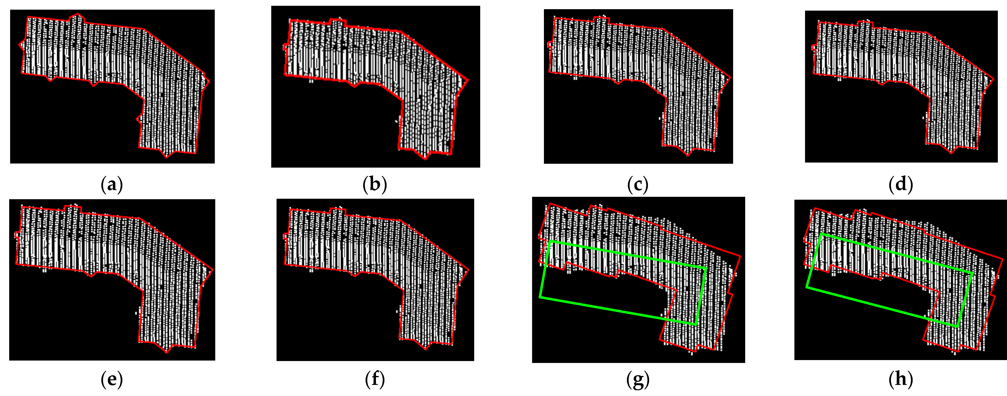
In the proposed method, the parameter ${\delta }_0$ determines the results of dominant direction detections, which directly relate to the regularization results. Therefore, rectangular and non-rectangular buildings are selected to study the parameter ${\delta }_0$. Results are shown in Figure 15 and Figure 16. It can be seen that approximately parallel or perpendicular initial dominant directions are not merged when ${\delta }_0$ is set as a small value (e.g., 1°, 5°). As a result, line segments of the rectangle building are not strictly parallel or perpendicular, see the rectangles in Figure 15b,c. When the ${\delta }_0$ value is set too large (e.g., 25°, 30°), originally non-parallel initial dominant directions are merged, leading to severe misalignment between the regularized outlines and the projected point clouds (see Figure 16g,h). This suggests that for rectangular buildings, ${\delta }_0$ should be larger than or equal to 10°. For non-rectangular buildings, it is recommended that ${\delta }_0\le 20°$. Based on the above analysis, we suggest tuning ${\delta }_0$ within the range [10$°$, 20$°$] and it is set as 10$°$ in all experiments.

6. Conclusions

Due to the complexity of building structures and point clouds, it is a challenging task to automatically extract building outlines from airborne LiDAR data. In the paper, an outline extraction method based on topology-aware loop parsing and parallel constraint is proposed. To reduce the impact of scattered point clouds, a constrained Delaunay triangulation (DT) is proposed to construct topological relationships between points. Subsequently, semantic loops are searched in a topologically aware manner from the undirected graph, and accurate boundary points are extracted via parsing loops. After that, dominant directions are obtained via angle normalization, merging, and perpendicular pairing. Finally, line segments are adjusted under parallel constraint according to unit length residual, which simultaneously considers boundary point distribution and line segment length. Experiments on five datasets verify that semantic boundary points can be accurately extracted. In addition, the extracted outlines are attractive, and most line segments are parallel and perpendicular. In terms of boundary point extraction precision, the average CP, CR, Q, and F₁ metric values are over 95.22%, 99.09%, 94.40%, and 97.11% in Vaihingen. And the average Q and F₁ metric values are 92.83% and 96.28% in New Zealand. For the outline extraction accuracy, the average RMSE, PoLiS, and RCC metric values are 0.81 m, 0.71 m, and 0.64 m in Vaihingen, 0.86 m, 0.55 m, and 0.56 m in New Zealand, respectively.

However, the proposed method can only extract linear outlines, and non-linear outlines cannot be perfectly extracted. Thus, we will attempt to extend the proposed method to more complex building outlines, e.g., curved outlines. In addition, two parameters (i.e., SF₀ and ${\delta }_0$) need to be preset according to parameter setting recommendations, which reduces the automation level of the proposed method. In the next step, we will attempt to construct an adaptive outline extraction method.

References

1. Huang, J.; Stoter, J.; Peters, R.; Nan, L. City3D: Large-scale building reconstruction from airborne LiDAR point clouds. Remote Sens. 2022, 14, 2254. [Google Scholar] [CrossRef]
2. Son, T.; Weedon, Z.; Yigitcanlar, T.; Corchado, T.; Mehmood, R. Algorithmic urban planning for smart and sustainable development: Systematic review of the literature. Sustain. Cities Soc. 2023, 94, 104562. [Google Scholar] [CrossRef]
3. Cao, Y.; Xu, C.; Aziz, N.; Kamaruzzaman, S. BIM–GIS integrated utilization in urban disaster management: The contributions, challenges, and future directions. Remote Sens. 2023, 15, 1331. [Google Scholar] [CrossRef]
4. Zang, D.; Wang, J.; Zhang, X.; Yu, J. Semantic extraction of roof contour lines from airborne LiDAR building point clouds based on multidirectional equal-width banding. IEEE J. Sel. Top. Appl. Earth Obs. Remote Sens. 2024, 17, 16316–16328. [Google Scholar] [CrossRef]
5. Du, J.; Chen, D.; Wang, R.; Peethambaran, J.; Mathiopoulos, P.; Xie, L.; Yun, T. A novel framework for 2.5-D building contouring from large-scale residential scenes. IEEE Trans. Geosci. Remote Sens. 2019, 57, 4121–4145. [Google Scholar] [CrossRef]
6. Lei, P.; Chen, Z.; Tao, R.; Li, J.; Hao, Y. Boundary recognition of ship planar components from point clouds based on trimmed Delaunay triangulation. Comput. Aided Des. Appl. 2025, 178, 103808. [Google Scholar] [CrossRef]
7. Bao, P.; Zhang, L.; Wu, X. Canny edge detection enhancement by scale multiplication. IEEE Trans. Pattern Anal. Mach. Intell. 2005, 27, 1485–1490. [Google Scholar] [CrossRef]
8. Remya, A.; Gopalan, S. Comparative analysis of eight direction Sobel edge detection algorithm for brain tumor MRI images. Procedia Comput. Sci. 2022, 201, 487–494. [Google Scholar] [CrossRef]
9. Bhardwaj, S.; Mittal, A. A survey on various edge detector techniques. Procedia Technol. 2012, 4, 220–226. [Google Scholar] [CrossRef]
10. Liao, Z.; Liu, J.; Shi, G.; Meng, J. Grid partition variable step alpha shapes algorithm. Math. Probl. Eng. 2021, 2021, 9919003. [Google Scholar] [CrossRef]
11. Chen, X.; Fang, F. Morphology-based scattered point cloud contour extraction. J. TongJi Univ. 2014, 42, 1738–1743. [Google Scholar] [CrossRef]
12. Piegl, L.; Tiller, W. Algorithm for finding all k nearest neighbors. Comput. Aided Des. 2002, 34, 167–172. [Google Scholar] [CrossRef]
13. Awrangjeb, M. Using point cloud data to identify, trace, and regularize the outlines of buildings. Int. J. Remote Sens. 2016, 37, 551–579. [Google Scholar] [CrossRef]
14. He, X.; Wang, R.; Feng, C.; Zhou, X. A novel type of boundary extraction method and its statistical improvement for unorganized point clouds based on concurrent Delaunay triangular meshes. Sensors 2023, 23, 1915. [Google Scholar] [CrossRef] [PubMed]
15. Wang, J.; Zang, D.; Yu, J.; Xie, X. Extraction of building roof contours from airborne LiDAR point clouds based on multidirectional bands. Remote Sens. 2024, 16, 190. [Google Scholar] [CrossRef]
16. Wu, C.; Chen, X.; Jin, T.; Hua, X.; Liu, W.; Liu, J.; Gao, Y.; Zhao, B.; Jiang, Y.; Hong, Q. UAV building point cloud contour extraction based on the feature recognition of adjacent points distribution. Measurement 2024, 230, 114519. [Google Scholar] [CrossRef]
17. Ni, H.; Lin, X.; Ning, X.; Zhang, J. Edge detection and feature line tracing in 3D-point clouds by analyzing geometric properties of neighborhoods. Remote Sens. 2016, 8, 710. [Google Scholar] [CrossRef]
18. Liu, Y.; Wang, C.; Gao, N.; Zhang, Z. Point cloud adaptive simplification of feature extraction. Opt. Precis. Eng. 2017, 25, 245–254. [Google Scholar] [CrossRef]
19. Sun, S.; Salvaggio, C. Aerial 3D building detection and modeling from airborne LiDAR point clouds. IEEE J. Sel. Top. Appl. Earth Obs. Remote Sens. 2013, 6, 1440–1449. [Google Scholar] [CrossRef]
20. Zhao, C.; Guo, H.; Wang, Y.; Lu, J. Building outer boundary extraction from ALS point clouds using neighborhood point direction distribution. Opt. Precis. Eng. 2021, 29, 374–387. [Google Scholar] [CrossRef]
21. Kirkpatrick, D.; Seidel, R. On the shape of a set of points in the plane. IEEE Trans. Inf. Theory 1983, 29, 551–559. [Google Scholar] [CrossRef]
22. Wu, Y.; Wang, L.; Hu, C.; Cheng, L. Extraction of building contour from airborne LiDAR point cloud using variable radius alpha shapes method. J. Image Graph. 2021, 26, 0910–0923. [Google Scholar] [CrossRef]
23. Wang, Z.; Ma, H.; Xu, H.; Yang, Z. Novel algorithm for fast extracting edges from massive point clouds. Comput. Eng. Appl. 2010, 46, 213–215. [Google Scholar] [CrossRef]
24. Liu, K.; Ma, H.; Zhang, L.; Gao, L.; Xiang, S.; Chen, D.; Miao, Q. Building outline extraction using adaptive tracing alpha shapes and contextual topological optimization from airborne LiDAR. Autom. Constr. 2024, 160, 105321. [Google Scholar] [CrossRef]
25. Santos, R.; Galo, M.; Carrilho, A. Extraction of building roof boundaries from LiDAR data using an adaptive alpha-shape algorithm. IEEE Geosci. Remote Sens. Lett. 2019, 16, 1289–1293. [Google Scholar] [CrossRef]
26. Qin, Z.; Liang, X.; Wang, J.; Gao, X.; Chen, X.; Yin, X.; Jia, H.; Liu, Y. Indoor 3D wireframe construction from incomplete point clouds based on Gestalt rules. Int. J. Appl. Earth Obs. Geoinf. 2024, 130, 103893. [Google Scholar] [CrossRef]
27. Li, Y.; Tan, D.; Gao, G.; Liu, R. Extraction of building contour from point clouds using dual threshold alpha shapes algorithm. J. Yangte River Sci. Res. Inst. 2016, 33, 1–4. [Google Scholar] [CrossRef]
28. Santos, R.; Pessoa, G.; Carrilho, A.; Galo, M. Automatic building boundary extraction from airborne LiDAR data robust to density variation. IEEE Geosci. Remote Sens. Lett. 2020, 19, 6500305. [Google Scholar] [CrossRef]
29. Yu, L.; Li, X.; Fu, C.; Cohen-Or, D.; Heng, P. EC-Net: An edge-aware point set consolidation network. In Proceedings of the European Conference on Computer Vision, Munich, Germany, 8–14 September 2018; pp. 386–402. [Google Scholar] [CrossRef]
30. Bazazian, D.; Parés, M. EDC-Net: Edge detection capsule network for 3D point clouds. Appl. Sci. 2021, 11, 1833. [Google Scholar] [CrossRef]
31. Zhang, Y.; Liu, Z.; Liu, T.; Peng, B.; Li, X.; Zhang, Q. Large-scale point cloud contour extraction via 3-D-guided multiconditional residual generative adversarial network. IEEE Geosci. Remote Sens. Lett. 2019, 17, 142–146. [Google Scholar] [CrossRef]
32. Hackel, T.; Wegner, J.; Schindler, K. Joint classification and contour extraction of large 3D point clouds. ISPRS J. Photogramm. Remote Sens. 2017, 130, 231–245. [Google Scholar] [CrossRef]
33. Yang, H.; Huang, S.; Wang, R. Efficient roof vertex clustering for wireframe simplification based on the extended multiclass twin support vector machine. IEEE Geosci. Remote Sens. Lett. 2024, 21, 6501405. [Google Scholar] [CrossRef]
34. Mehri, S.; Hooshangi, N.; Mahdizadeh, N. A novel context-aware Douglas–Peucker (CADP) trajectory compression method. ISPRS Int. J. Geoinf. 2025, 14, 58. [Google Scholar] [CrossRef]
35. Liu, C.; Li, N.; Wu, H.; Yang, X. Adjustment model of boundary extraction for urban complicated building based on LiDAR data. J. Tongji Univ. 2012, 40, 1399–1405. [Google Scholar] [CrossRef]
36. Park, W.; Yu, K. Hybrid line simplification for cartographic generalization. Pattern Recognit. Lett. 2011, 32, 1267–1273. [Google Scholar] [CrossRef]
37. Rangayyan, R.; Guliato, D.; Carvalho, J.; Santiago, S. Polygonal approximation of contours based on the turning angle function. J. Electron. Imaging 2008, 17, 023016. [Google Scholar] [CrossRef]
38. Li, X.; Qiu, F.; Shi, F.; Tang, Y. A recursive hull and signal-based building footprint generation from airborne LiDAR data. Remote Sens. 2022, 14, 5892. [Google Scholar] [CrossRef]
39. Sampath, A.; Shan, J. Building boundary tracing and regularization from airborne LiDAR point clouds. Photogramm. Eng. Remote Sens. 2007, 73, 805–812. [Google Scholar] [CrossRef]
40. Zhao, Z.; Duan, Y.; Zhang, Y.; Cao, R. Extracting buildings from and regularizing boundaries in airborne lidar data using connected operators. Int. J. Remote Sens. 2016, 37, 889–912. [Google Scholar] [CrossRef]
41. Kwak, E.; Habib, A. Automatic representation and reconstruction of DBM from LiDAR data using recursive minimum bounding rectangle. ISPRS J. Photogramm. Remote Sens. 2014, 93, 171–191. [Google Scholar] [CrossRef]
42. Feng, M.; Zhang, T.; Li, S.; Jin, G.; Xia, Y. An improved minimum bounding rectangle algorithm for regularized building boundary extraction from aerial LiDAR point clouds with partial occlusions. Int. J. Remote Sens. 2020, 41, 300–319. [Google Scholar] [CrossRef]
43. Xie, L.; Zhu, Q.; Hu, H.; Wu, B.; Li, Y.; Zhang, Y.; Zhong, R. Hierarchical regularization of building boundaries in noisy aerial laser scanning and photogrammetric point clouds. Remote Sens. 2018, 10, 1996. [Google Scholar] [CrossRef]
44. Poullis, C. A framework for automatic modeling from point cloud data. IEEE Trans. Pattern Anal. Mach. Intell. 2013, 35, 2563–2575. [Google Scholar] [CrossRef] [PubMed]
45. Albers, B.; Kada, M.; Wichmann, A. Automatic extraction and regularization of building outlines from airborne LiDAR point clouds. Int. Arch. Photogramm. Remote Sens. Spat. Inf. Sci. 2016, 41, 555–560. [Google Scholar] [CrossRef]
46. Xia, S.; Chen, D.; Wang, R.; Li, J.; Zhang, X. Geometric primitives in LiDAR point clouds: A review. IEEE J. Sel. Top. Appl. Earth Obs. Remote Sens. 2020, 13, 685–707. [Google Scholar] [CrossRef]
47. Shewchuk, J. Delaunay refinement algorithms for triangular mesh generation. Comput. Geom. 2002, 22, 21–74. [Google Scholar] [CrossRef]
48. Sarrate, J.; Palau, J.; Huerta, A. Numerical representation of the quality measures of triangles and triangular meshes. Commun. Numer. Methods Eng. 2003, 19, 551–561. [Google Scholar] [CrossRef]
49. Chen, Q.; Wang, L.; Waslander, S.; Liu, X. An end-to-end shape modeling framework for vectorized building outline generation from aerial images. ISPRS J. Photogramm. Remote Sens. 2020, 170, 114–126. [Google Scholar] [CrossRef]
50. Lu, Y.; Shapiro, L. Closing the loop for edge detection and object proposals. In Proceedings of the Conference on Association for the Advancement of Artificial Intelligence, San Francisco, CA, USA, 4–9 February 2017; pp. 4204–4210. [Google Scholar] [CrossRef]
51. Gao, F.; Wang, M.; Cai, Y.; Lu, S. Extracting closed object contour in the image: Remove, connect and fit. Pattern Anal. Appl. 2019, 22, 1123–1136. [Google Scholar] [CrossRef]
52. Dillenburg, J.; Nelson, P. Improving the efficiency of depth-first search by cycle elimination. Inf. Process. Lett. 1993, 45, 5–10. [Google Scholar] [CrossRef]
53. Taleghani, M.; Tenpierik, M.; Dobbelsteen, A. Environmental impact of courtyards—A review and comparison of residential courtyard buildings in different climates. J. Green Build. 2012, 7, 113–136. [Google Scholar] [CrossRef]
54. Markus, B. A review on courtyard design criteria in different climatic zones. Afr. Res. Rev. 2016, 10, 181–192. [Google Scholar] [CrossRef]
55. Asuero, A.; González, G. Fitting straight lines with replicated observations by linear regression. III. Weighting data. Crit. Rev. Anal. Chem. 2007, 37, 143–172. [Google Scholar] [CrossRef]
56. Zhou, Q.; Neumann, U. Complete residential urban area reconstruction from dense aerial LiDAR point clouds. Graph. Models. 2013, 75, 118–125. [Google Scholar] [CrossRef]
57. Zhang, K.; Yan, J.; Chen, S. Automatic construction of building footprints from airborne LIDAR data. IEEE Trans. Geosci. Remote Sens. 2006, 44, 2523–2533. [Google Scholar] [CrossRef]
58. Wei, J.; Wu, H.; Yue, H.; Jia, S.; Li, J.; Liu, C. Automatic extraction and reconstruction of a 3D wireframe of an indoor scene from semantic point clouds. Int. J. Digit. Earth 2023, 16, 3239–3267. [Google Scholar] [CrossRef]
59. Shen, W.; Li, J.; Chen, Y.; Deng, L.; Peng, G. Algorithms study of building boundary extraction and normalization based on LiDAR data. Int. J. Remote Sens. 2008, 12, 692–698. [Google Scholar] [CrossRef]
60. Awrangjeb, M.; Fraser, C. An automatic and threshold-free performance evaluation system for building extraction techniques from airborne LiDAR data. IEEE J. Sel. Top. Appl. Earth Obs. Remote Sens. 2014, 7, 4184–4198. [Google Scholar] [CrossRef]
61. Powers, D. Evaluation: From precision, recall and F-measure to ROC, informedness, markedness and correlation. J. Mach. Learn. Technol. 2011, 2, 37–63. [Google Scholar] [CrossRef]
62. Baswana, S.; Chaudhury, S.; Choudhary, K.; Khan, S. Dynamic DFS in undirected graphs: Breaking the O(m) barrier. SIAM J. Comput. 2019, 48, 1335–1363. [Google Scholar] [CrossRef]
63. Jawarneh, A.; Foschini, L.; Bellavista, P. Polygon simplification for the efficient approximate analytics of georeferenced big data. Sensors 2023, 23, 8178. [Google Scholar] [CrossRef]
64. Calasan, M.; Aleem, S.; Zobaa, A. On the root mean square error (RMSE) calculation for parameter estimation of photovoltaic models: A novel exact analytical solution based on Lambert W function. Energy Convers. Manag. 2020, 210, 112716. [Google Scholar] [CrossRef]
65. Widyaningrum, E.; Peters, R.; Lindenbergh, R. Building outline extraction from ALS point clouds using medial axis transform descriptors. Pattern Recognit. 2020, 106, 107447. [Google Scholar] [CrossRef]
66. Avbelj, J.; Müller, R.; Bamler, R. A metric for polygon comparison and building extraction evaluation. IEEE Geosci. Remote Sens. Lett. 2014, 12, 170–174. [Google Scholar] [CrossRef]
67. Dey, E.; Awrangjeb, M. A robust performance evaluation metric for extracted building boundaries from remote sensing data. IEEE J. Sel. Top. Appl. Earth Obs. Remote Sens. 2020, 13, 4030–4043. [Google Scholar] [CrossRef]
68. Awrangjeb, M.; Lu, G.; Fraser, C. Automatic building extraction from LiDAR data covering complex urban scenes. Int. Arch. Photogramm. Remote Sens. Spat. Inf. Sci. 2014, 40, 25–32. [Google Scholar] [CrossRef]
69. Kong, G.; Fan, H.; Lobaccaro, G. Automatic building outline extraction from ALS point cloud data using generative adversarial network. Geocarto Int. 2022, 37, 15964–15981. [Google Scholar] [CrossRef]
Figure 1. Workflow of the proposed method.
Remotesensing 17 03498 g001
Figure 2. Constrained Delaunay triangulation (DT). (a) DT without constraints; (b) DT under shape constraint; (c) DT under side length constraint; (d) DT under shape and side length constraints. (Triangles within the yellow ellipses are unnecessary triangles, while triangles within the red ellipses are large triangles.).
Remotesensing 17 03498 g002
Figure 3. Boundary edge and boundary point extraction. (Triangle containing the two points within the red ellipse is removed. Points A, B, C, D are boundary points, T1 and T2 denote two triangles formed by these four boundary points respectively.).
Remotesensing 17 03498 g003
Figure 4. Topology-aware loop extraction. (a) Image and projected point clouds; (b) Boundary point and boundary edge extraction; (c,d) are the loop extraction results of different projected point clouds. (Yellow ellipses in Figure (a) mark the holes in the point clouds and yellow ellipses Figure (b) mark the detected loops.).
Remotesensing 17 03498 g004
Figure 5. Topology-aware loop extraction. (a) Building A; (b) Building B; (c) Building C.
Remotesensing 17 03498 g005
Figure 6. MBR. (a) Building A; (b) Extracted boundary points; (c) MBR of hole boundary points; (d) Building B; (e) Extracted boundary points; (f) MBR of courtyard boundary points.
Remotesensing 17 03498 g006
Figure 7. False boundary point elimination. (a) Constrained DT; (b) Before elimination; (c) After elimination. (In Figure (a), the triangle containing two closed points in the yellow ellipse is removed. In Figure (b), the numbers denote the sequence number of the boundary points, and point 6 in the yellow ellipse is the false boundary point.).
Remotesensing 17 03498 g007
Figure 8. Normalization of dominant direction angles. (a) Building image; (b) Projected point clouds of a complex building; (c) Angle distribution before normalization; (d) Angle distribution after normalization.
Remotesensing 17 03498 g008aRemotesensing 17 03498 g008b
Figure 9. Test datasets. (a) Area 1; (b) Area 2; (c) Area 3; (d) Area 4; (e) Area 5.
Remotesensing 17 03498 g009
Figure 10. Boundary point extraction results. (a) Area 1; (b) Area 2; (c) Area 3; (d) Area 4; (e) Area 5.
Remotesensing 17 03498 g010
Figure 11. (AF) Comparison results of selected buildings. (Green rectangles denote the erroneous boundary points and the blue rectangles represent the omitted boundary points.).
Remotesensing 17 03498 g011
Figure 12. Outline extraction results. (a) Area 1; (b) Area 2; (c) Area 3; (d) Area 4; (e) Area 5.
Remotesensing 17 03498 g012
Figure 13. (AF) Comparison results of selected buildings.
Remotesensing 17 03498 g013
Figure 14. Constrained DT for different SF0. (ai) correspond to SF0 values of 0.1, 0.2, 0.3, 0.35, 0.4, 0.5, 0.55, 0.6, and 0.8.
Remotesensing 17 03498 g014
Figure 15. Rectangle building outline regularization with different δ 0 values. (a) References. (bh) correspond to δ 0 values of 1°, 5°, 10°, 15°, 20°, 25°, and 30°. (Line segments within the green rectangles are not strictly parallel or perpendicular.).
Remotesensing 17 03498 g015
Figure 16. Non-rectangle building outline regularization with different δ 0 values. (a) References. (bh) correspond to δ 0 values of 1°, 5°, 10°, 15°, 20°, 25°, and 30°.
Remotesensing 17 03498 g016