Quantifying Climate-Anthropogenic Forcing on Arid Basin Vegetation Dynamics Using Multi-Vegetation Indices and Geographical Detector

Highlights

What are the main findings?

• Vegetation in the Heihe River Basin exhibited an overall upward trend, with significant regional variation during 2004–2023.
• Land use change and water management policies dominated non-climatic impacts on vegetation change.

What is the implication of the main finding?

• The enhancement of ecological governance is necessary through tailoring it to local conditions.
• Balancing agricultural and ecological water use in the basin is key to its ecological stability.

Abstract

Understanding the spatiotemporal dynamics of vegetation and their driving mechanisms is essential for ecological assessment and management. However, current assessments of the Heihe River Basin (HRB) vegetation dynamics remain uncertain due to reliance on single indices without cross-validation and oversimplified attribution of residual variations. Here, we integrated four complementary vegetation indices (NDVI, EVI, kNDVI, and NIRv) with trend and abrupt change detection analyses to establish a framework for assessing vegetation changes in the HRB from 2004 to 2023. Given that the dominance of non-climatic factors is widely attributed to human water management and land use policies, land use change and other anthropogenic factors were incorporated together with topographic/edaphic factors into the optimal parameter-based geographical detector (OPGD), where vegetation changes induced by non-climatic factors were first isolated through residual trend analysis, thereby quantifying their explanatory power on vegetation index variations. The results demonstrate that vegetation in the HRB experienced a fluctuating upward trend (0.0013/yr) from 2004 to 2023, with significant improvement in 43% and degradation in 3% of the region. Climatic and non-climatic factors explained 26% and 74% of spatial variation, dominated by precipitation and land use change, respectively. Notably, the interaction of land use change and elevation accounted for 56% of NIRv variation, markedly exceeding single factors, as determined by the interaction detector in the OPGD. Additionally, large-scale ecological restoration projects and effective water resource management policies have played a pivotal role in facilitating vegetation recovery across the basin. This study enhances insight into vegetation dynamics and supports both sustainable restoration and development in the HRB.

1. Introduction

As an essential component of terrestrial ecosystems, vegetation plays a key role in material and energy balance, soil and water conservation, windbreak and sand fixation, and climate regulation [1,2]. At the same time, vegetation demonstrates high dependence and sensitivity to various natural and anthropogenic factors, enabling it to reflect the effects of climate change and human activities over short time scales, particularly in arid and semi-arid regions [3,4]. For instance, in the arid HRB, vegetation shows a high interannual NDVI variability [5], while hydrological processes also fluctuate strongly under human activities and extreme events [6,7]. Existing research suggests that drought is expected to increase with climate change, potentially expanding drylands to cover more than half of the Earth’s land surface by 2100 [8]. Therefore, studying long-term vegetation dynamics in arid and semi-arid regions is of great significance for gaining deeper insights into the response processes of fragile ecosystems to climate change and human disturbances [9], enhancing regional ecosystem adaptability and resilience [10], optimizing land resource allocation and ecological management strategies [11], and promoting the sustainable development of terrestrial ecosystems [12].

Remote sensing technology provides an effective approach for large-scale, long-term vegetation monitoring. Multi-source remote sensing data facilitate continuous monitoring of vegetation dynamics and related indicators, providing indirect insights into ecosystem functions, with advantages such as spatial continuity, high temporal resolution, and strong reproducibility [13]. Among various remote sensing products, Moderate Resolution Imaging Spectroradiometer (MODIS) data—with its high temporal resolution and cost-effectiveness—has become a widely used tool for monitoring vegetation changes at global and regional scales [14,15]. As a result, MODIS data has played a central role in regional ecological studies focusing on vegetation dynamics and their driving mechanisms [16].

Several vegetation indices have been developed based on satellite remote sensing, including the normalized difference vegetation index (NDVI), enhanced vegetation index (EVI), kernel NDVI (kNDVI), and near-infrared reflectance of vegetation (NIRv). Among these, NDVI remains the most fundamental and widely used index, though it suffers from saturation effects in dense vegetation and significant interference from soil background and atmospheric conditions [17]. EVI incorporates the blue band for atmospheric correction and soil suppression, making it more suitable for high-density vegetation areas such as forests and croplands [18]. NIRv demonstrates reduced interference from soil brightness and enhanced capability to capture changes in structurally complex landscapes [19]. The recently developed kNDVI introduces nonlinear features through kernel functions to better characterize the complex relationship between NDVI and vegetation productivity, thereby improving estimation accuracy [20]. However, comprehensive comparative evaluations of vegetation indices remain limited in the HRB, where most studies still rely on a single index [21,22] without multi-index cross-validation. The application of individual vegetation indices in this heterogeneous watershed often introduces systematic biases due to their inherent limitations. For example, NDVI demonstrates susceptibility to soil background effects in sparsely vegetated downstream areas and saturation effects in densely vegetated midstream oasis farmlands [23,24]. These constraints may compromise the accuracy of vegetation dynamic assessments across different watershed sections, ultimately affecting the reliability of ecological process studies.

Climate change exerts significant impacts on vegetation at both global and regional scales, with temperature and precipitation serving as key determinants of vegetation growth [25,26]. For instance, increasing temperature prolongs the growing season, particularly in high-latitude and high-altitude regions, significantly stimulating vegetation growth [27,28]. Increased precipitation markedly enhances vegetation growth in northwestern Ethiopia, exhibiting a one-month lag effect [29]. Non-climatic factors also play an important role in vegetation change [30]. Among non-climatic factors, topography plays an indispensable role in regulating vegetation spatial patterns. For example, Liang et al. (2024) [31] demonstrated that high-altitude and steep areas exhibit sparse vegetation, while lowlands and gentle slopes support denser vegetation coverage. Additionally, human activities constitute critical drivers of vegetation growth and degradation [32]. Numerous studies demonstrate that overexploitation and overgrazing have degraded grasslands in Central Asia and Mongolia [13,33], while China’s Grain to Green Program (GTGP) has significantly improved vegetation coverage on the Loess Plateau [34]. Furthermore, low soil moisture and high vapor pressure deficit can substantially suppress vegetation productivity anomalies [35], whereas elevated atmospheric CO₂ concentrations represent a major driver of global-scale vegetation changes [36]. Consequently, quantitative assessment of climate change versus human-dominated non-climatic impacts on vegetation dynamics has attracted widespread attention.

Under the complex interplay of climatic and non-climatic factors, direct analysis of VI trends often fails to identify their respective contributions to vegetation dynamics. The multiple regression residual analysis method addresses this by first establishing multivariate relationships between VIs and climatic factors (e.g., precipitation, temperature), then attributing the residuals to non-climatic factors (e.g., human activity), thereby enabling a quantitative assessment of the relative contributions of climatic and non-climatic drivers [37]. This approach has gained extensive application, as exemplified by Ren et al. (2022) [12] quantifying 34% and 66% contributions from climatic and non-climatic factors respectively in the Yellow River Basin. Notably, while residual analysis proves practical for partitioning climatic and non-climatic drivers, most studies simply assume that non-climatic residuals represent human activity proxies [38]. This assumption neglects other non-climatic factors (e.g., topography, soil, hydrology), especially in complex heterogeneous regions [39,40]. Crucially, this method also fails to capture the interactive effects where climate variability influences human activity, which in turn drives vegetation change [41]. The optimal parameter-based geographical detector (OPGD) offers a spatial statistical approach to quantify explanatory power (q-value) and detect nonlinear interactions through optimal stratification strategies [42]. This method is particularly effective in identifying dominant mechanisms and elucidating coupled effects under complex geographical contexts. In our study, it was further applied to explore specific factors within the overall non-climatic drivers derived from multiple regression residual analysis [43,44].

The HRB represents a typical inland arid and semi-arid basin and ranks as China’s second largest endorheic watershed. From its upper to lower reaches, the basin exhibits diverse landscapes encompassing glaciers/permafrost, forests, meadows, artificial/natural oases, deserts, and lakes [45]. This ecosystem demonstrates inherent ecological sensitivity and vulnerability [46]. Since the 1960s, intensified climate change combined with agricultural expansion and rapid urbanization in midstream areas has dramatically increased regional water and land resource demands, leading to multiple ecological stressors including groundwater depletion, desertification, salinization, and grassland degradation [47]. To mitigate ecological deterioration, the Chinese government has implemented major restoration projects since 2000, including the Grazing Prohibition/Grassland Restoration Program, ecological water diversion, key shelterbelt construction, and terminal lake protection. Among these, the Ecological Water Diversion Project (EWDP) has served as a central initiative, playing a critical role in mitigating ecological degradation in the downstream areas by reallocating water resources within the basin [48]. Through administrative regulation and scientific management, the project aims to transfer a portion of agricultural water from the midstream to the downstream regions, thereby restoring dried-up river channels, replenishing depleted aquifers, and rescuing endangered desert vegetation ecosystems [49]. These measures have effectively alleviated downstream ecological crises and significantly improved regional environments [50]. Hence, long-term spatiotemporal analysis of vegetation dynamics in the HRB is essential for evaluating the effectiveness of past ecological restoration efforts and informing the planning and management of future initiatives.

The aims of this study were to: (1) comprehensively assess the spatiotemporal changes in vegetation across the HRB from 2004 to 2023 using four vegetation indices (NDVI, EVI, kNDVI, and NIRv); (2) quantify the relative contributions of climatic and non-climatic factors to vegetation changes; (3) identify the dominant climatic drivers and investigate the effects of human activities and other non-climatic factors, including their interactions, on vegetation dynamics; (4) discuss the impacts of ecological engineering and policies on vegetation dynamics. This study deepens the understanding of vegetation dynamics and their underlying mechanisms, offering guidance for sustainable vegetation development in the HRB.

2. Materials and Methods

2.1. Study Area

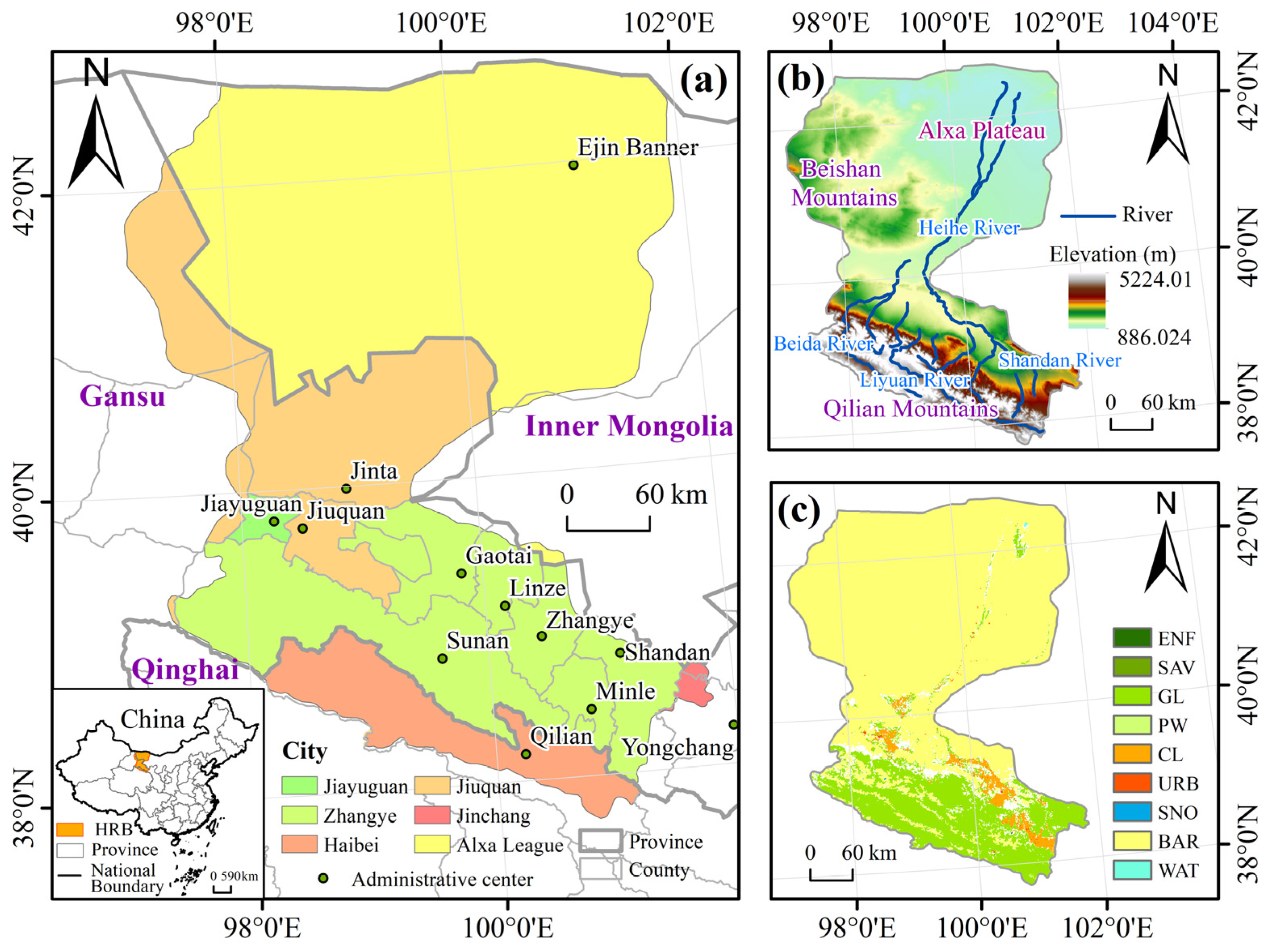
The HRB is located in the arid and semi-arid regions of Northwest China (37.7° to 42.7°N and 97.1° to 102.0°E, Figure 1a). It is the second largest inland river basin in the country, spanning Qinghai Province, Gansu Province, and the Inner Mongolia Autonomous Region (Figure 1b) and covering an area of approximately 143,000 km² [45]. The elevation of the HRB increases from north to south, ranging from 886 m to 5224 m, which contributes to the formation of a typical mountain–oasis–desert system [51].

The land use and cover types in the HRB are diverse (Figure 1c). In the upstream region, the dominant types include grasslands (GL), permanent snow and ice (SNO), and evergreen needleleaf forests (ENF). GL is primarily composed of alpine meadows, covers 10.1% of the area, while SNO and ENF, mainly represented by Qinghai spruce, each account for approximately 0.5%. The midstream region is characterized by a mosaic of croplands (CL) and barren lands (BAR). CL, dominated by maize fields, occupies 3.6% of the area, whereas BAR, largely consisting of piedmont desert, extends across 29.4%. In the downstream region, BAR becomes even more prominent, covering 55.1% of the area and primarily consisting of desert landscapes. Other land covers include Savanna (SAV, 0.2%), with representative species such as Populus euphratica and Tamarix, as well as water bodies (WAT), mainly terminal lakes, occupying 0.3%. Additionally, urban and built-up lands (URB), encompassing cities, towns, and residential areas, contribute 0.3% of the total land cover across the basin [45].

2.2. Data Sources

2.2.1. Vegetation Index

We utilized the Moderate-resolution Imaging Spectroradiometer (MODIS) surface reflectance product MCD43A4 on the Google Earth Engine (GEE) platform (https://earthengine.google.com (accessed on 22 August 2024)) to derive vegetation indices including NDVI, EVI, kNDVI, and NIRv. This product provides surface reflectance for seven spectral bands at a spatial resolution of 500 m. The reflectance values have been corrected using a bidirectional reflectance distribution function (BRDF), which reduces the influence of varying illumination and observation geometries [52].

The normalized difference vegetation index (NDVI) is calculated from the near-infrared (NIR: MCD43A4 Band 2) and red (Red: MCD43A4 Band 1) surface reflectance [53]:

$$NDVI={\displaystyle \frac{\left(NIR-Red\right)}{\left(NIR+Red\right)}}$$

(1)

The enhanced vegetation index (EVI) improves vegetation detection in high biomass regions by correcting for atmospheric aerosol and soil background effects by incorporating the blue band (MCD43A4 Band 3) and a soil adjustment factor [23]. It is defined as:

$$EVI=2.5\times {\displaystyle \frac{NIR-Red}{NIR+6\times Red-7.5\times Blue+1}}$$

(2)

The kernel normalized difference vegetation index (kNDVI) represents a nonlinear extension of NDVI, introduced to better capture complex relationships between vegetation structure and spectral response [20]. It is expressed as:

$$kNDVI=\tanh \left({\left({\displaystyle \frac{NIR-Red}{2\sigma }}\right)}^2\right)$$

(3)

where $\sigma$ denotes a tunable length-scale parameter designed to capture the nonlinear response of NDVI to vegetation density. According to Camps-Valls et al. (2021) [20], we adopt the formulation $\mathsf{\sigma }=0.5\left(\mathrm{N}\mathrm{I}\mathrm{R}-\mathrm{R}\mathrm{e}\mathrm{d}\right)$, which simplifies the expression to $kNDVI=tanh\left({\left(NDVI\right)}^2\right)$.

NIRv is intended to more accurately capture the vertical distribution of canopy photosynthetic activity and is computed as the product of NDVI and the NIR reflectance [19]. It is expressed as:

$$NIRv=\left(NDVI-0.08\right)\times NIR$$

(4)

The VIs were composited at both monthly and annual scales using the maximum value composite (MVC) method on the GEE platform, and subsequently resampled to a spatial resolution of 1000 m using bilinear interpolation. The MVC approach was adopted due to its capacity to mitigate the effects of clouds, atmospheric noise, and solar elevation angle [54]. To represent interannual variations in vegetation growth, the average of monthly maximum value composites of VIs during the growing season (April to October) was used as a proxy for annual vegetation status. Annual MVC VIs were utilized to perform trend analysis and to reveal the spatial patterns of vegetation change across the HRB.

2.2.2. LULC Data

The land use and land cover (LULC) data used in this study were derived from the MCD12Q1 product (https://search.earthdata.nasa.gov/ (accessed on 23 August 2024)), which provides annual global classifications at 500 m resolution. We primarily adopted the IGBP classification scheme [55] for categorization, as shown in Figure 1c, to analyze vegetation spatiotemporal characteristics in different LULC zones. Notably, in subsequent geographical detector, in order to facilitate the analysis of land use and land cover change (LUCC), the dataset was reclassified into six major categories: forest, grassland, water area, cropland, construction land, and unused land using ArcGIS (v10.8) [56]. In this study, forest corresponds to ENF; grassland includes GL and SAV; water area consists of PW and WAT; cropland corresponds to CL; Construction land corresponds to URB; and unused land comprises BAR and SNO.

2.2.3. AGPP Data

The annual gross primary productivity (AGPP) dataset for China’s terrestrial ecosystems (2000–2020) was developed by Xue et al. (2023) [57] using a random forest model based on ChinaFLUX tower observations and multiple variables, including biological, climatic, and soil factors. This approach resulted in a 30 arc-second resolution GeoTIFF dataset that robustly captures the spatial and temporal patterns of productivity across China. Given that the AGPP estimates are grounded in empirical site-level observations that incorporate data from 166 flux sites and 872 annual records, this dataset offers a reliable reference for evaluating satellite-based VIs.

To extend the temporal coverage through 2023, we utilized global GPP data from the Penman–Monteith–Leuning model (PML_V2 0.1.8) [58], which was obtained from the GEE platform. We established separate correction equations for different land cover types to improve the consistency between the PML_V2 and ChinaFLUX AGPP datasets during their overlapping period (2004–2020). This correction process significantly enhanced the data agreement, with the global R² increasing from 0.44 to 0.78. The corrected PML_V2 GPP data were then used to fill the temporal gap for the years 2021–2023. The specific correction equations and a detailed accuracy assessment are provided in the Supplementary Materials (see Tables S1 and S2). This study systematically assessed the correlations between VIs and AGPP through linear regression analysis, based on a seamlessly integrated AGPP time series (2000–2023).

2.2.4. Climate Data

The climate data used in this study included temperature and precipitation, both obtained from a 1 km monthly climate dataset for China spanning 1901–2023 [59], provided by the National Earth System Science Data Center (https://www.geodata.cn/ (accessed on 22 August 2024)). The temperature and precipitation datasets, originally in NetCDF format, were processed using Python (v3.10) to convert them into GeoTIFF format. For the years 2004–2023, monthly values were averaged to generate annual mean temperature and precipitation maps, yielding 20 annual images for each dataset.

2.2.5. Topographic, Soil, and Human Activity Data

The digital elevation model (DEM) data was obtained from the USGS SRTMGL1 v003 dataset (https://lpdaac.usgs.gov/products/srtmgl1v003/ (accessed on 24 August 2024)) through the GEE platform. This dataset is part of the Shuttle Radar Topography Mission (SRTM) conducted by NASA and the USGS and provides near-global coverage of digital elevation data at a spatial resolution of 30 m [60]. Furthermore, regional slope and aspect were calculated from DEM data using ArcGIS (v10.8).

The soil texture classification data used in this study was obtained from the global soil texture map provided by OpenLandMap (https://stac.openlandmap.org/ (accessed on 26 August 2024)), which is based on the USDA soil texture classification system. The dataset has a spatial resolution of 250 m. The 0–5 cm depth layer of the soil texture data was used in this study. The soil moisture data (0–7 cm depth) was obtained from the ECMWF ERA5-Land monthly dataset (https://cds.climate.copernicus.eu/ (accessed on 26 August 2024)).

For population distribution data, we used the LandScan Global dataset from Oak Ridge National Laboratory (https://landscan.ornl.gov/ (accessed on 27 August 2024)), which offers global population estimates with a spatial resolution of 1 km. The nighttime light data were derived from the improved DMSP-OLS-like annual series for China (1992–2024) at 1 km spatial resolution [61], which integrates observations from DMSP-OLS and SNPP-VIIRS sensors. We selected data from 2004 to 2023 and calculated the multi-year average of annual values. The pixel values are unitless digital numbers (DN) that represent relative brightness. These data are summarized in

Table 1. Non-climatic driving factors of vegetation dynamics.

Categories	Factor	Abbreviation	Unit
Topography	Aspect	Asp	°
	Slope	Slp	°
	Elevation	Elev	m
Soil	Soil texture	Soilt	Categorical
	Soil moisture	Soilm	m3/m3
Human activity	Nighttime light	NTL	DN
	Population density	Popd	person/km2
	Land use change	LUC	Categorical

.

2.3. Methods

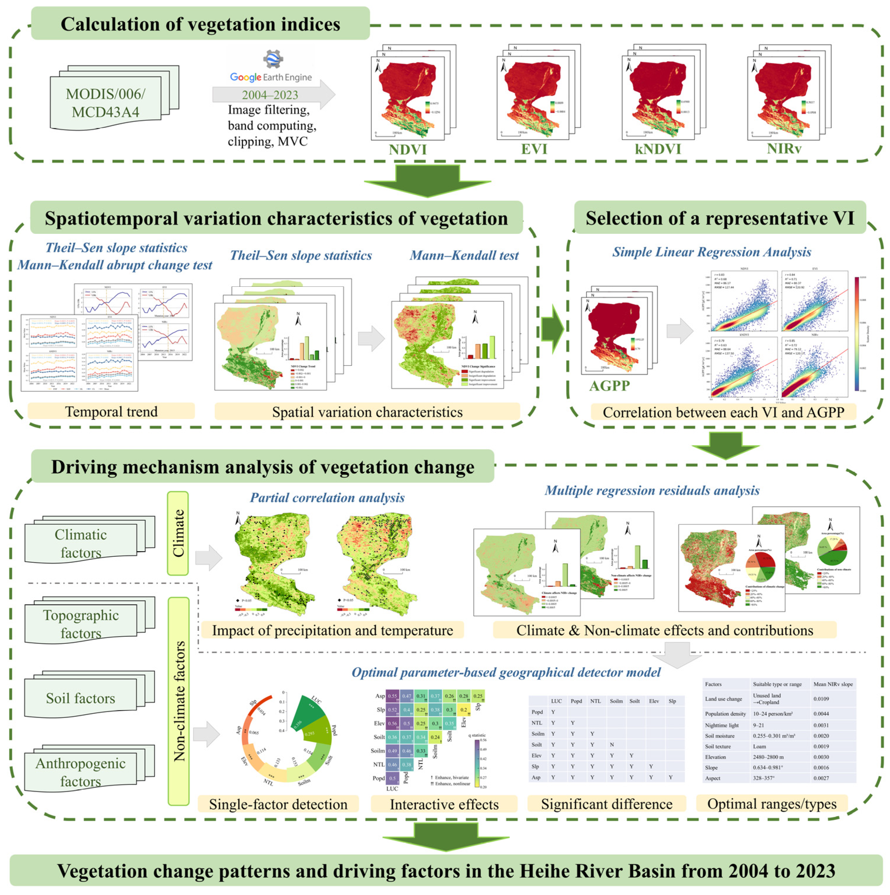
This study first derived four vegetation indices (NDVI, EVI, kNDVI, and NIRv) from MCD43A3 surface reflectance data spanning the period 2004–2023. The Theil–Sen trend analysis, Mann–Kendall significance test, and abrupt change test were then applied to examine the spatiotemporal variations in vegetation cover across the HRB over the past two decades. Linear regression models were established between the four vegetation indices and ChinaFLUX-derived AGPP to identify the most representative index for subsequent attribution analysis. To investigate the dominant climatic drivers of vegetation dynamics, partial correlation analysis was performed. Additionally, residual trend analysis was used to isolate vegetation changes attributed to non-climatic factors. Finally, the OPGD model quantified the contributions of topography, soil properties, and human activities to vegetation variation. The overall research framework is shown in Figure 2.

2.3.1. Theil–Sen Slope Statistics

Theil–Sen slope statistics is a non-parametric statistical method developed by Henri Theil and Pranab K. Sen [62]. Unlike traditional parametric approaches, it rarely assumes normal distribution or serial autocorrelation in the time series, thus proves particularly robust in handling small outliers and noise caused by missing values. This study adopts the Theil–Sen slope statistics to quantify trends in VIs, including NDVI, EVI, kNDVI, and NIRv. Specifically, the method computes the slope between all possible pairs of observations within the time series and derives the overall trend from the median of these slopes. The computation process proceeds as follows:

$$\beta =\mathrm{Median}\left({\displaystyle \frac{X_j-X_i}{j-i}}\right),\forall j>i$$

(5)

where $\beta$ represents the median slope of all computed pairwise differences within the time series. If $\beta$ > 0, the VI exhibits an increasing trend, whereas if $\beta$ < 0, it indicates a decreasing trend. $X_i$ and $X_j$ denote two observations in the time series, and $\mathrm{Median}$ represents the central value of the computed slopes.

2.3.2. Mann–Kendall Test

The Mann–Kendall (M-K) test, a non-parametric statistical method, complements Theil–Sen slope statistics for assessing trend significance in time series data [63]. This study employed the M-K test to evaluate the statistical significance of VI trends. The computation is as follows:

$$S=\sum _{i=1}^{n-1}\sum _{j=i+1}^n\mathrm{sign}\left(X_j-X_i\right)$$

(6)

$$sign(X_j-X_i)\left\{\begin{array}{c}1,X_j-X_i>0\\ 0,X_j-X_i=0\\ -1,X_j-X_i<0\end{array}\right.$$

(7)

$$var\left(S\right)={\displaystyle \frac{n\left(n-1\right)\left(2n+5\right)}{18}}$$

(8)

$$Z=\left\{\begin{array}{cc}{\displaystyle \frac{S-1}{\sqrt{var\left(S\right)}}},\hfill & S>0\hfill \\ \hspace{1em} 0\hspace{1em} ,\hfill & S=0\hfill \\ {\displaystyle \frac{S+1}{\sqrt{var\left(S\right)}}},\hfill & S<0\hfill \end{array}\right.$$

(9)

where $S$ denotes the test statistics, $n$ represents the total number of observations in the time series dataset, $sign$ denotes the sign function, and $X_i$ and $X_j$ correspond to the individual data points within the sampled time series. In this study, a 95% confidence level $(\left|Z\right|\ge 1.96)$ is employed to assess the statistical significance of vegetation trend detection. When the absolute value of the standardized test statistic $\left|Z\right|$ exceeds the critical thresholds of 1.96, the detected trend is statistically significant at the confidence level of 95%. Based on the calculation results, the Trend Results through the M-K test are divided into 4 levels (

Table 2. The classification of vegetation change.

Impact Level	p-Value	Theil–Sen Slope
Significant degradation	<0.05	<0
Insignificant degradation	>0.05	<0
Significant improvement	<0.05	>0
Insignificant improvement	>0.05	>0

).

2.3.3. Mann–Kendall Abrupt Change Test

The M-K abrupt change test serves as a robust non-parametric statistical tool for detecting significant shifts within time series data, widely applied in climate diagnostics and ecological trend assessments [64]. This method captures both the temporal and spatial distribution of abrupt changes through the construction of two standardized statistic sequences, UF and UB. In this study, the M-K test was applied to identify potential trend shifts in VIs across the HRB, aiming to reveal temporal discontinuities in vegetation dynamics under environmental influences. For a given time series $\mathrm{x}$ with $n$ sample points, the test constructs an ordered sequence as follows:

$$S_k=\sum _{i=1}^k{r}_i,r_i=\left\{\begin{array}{c}1,x_i>x_j\\ 0,x_i\le x_j\end{array},j=\mathrm{1,2},\cdots ,i\right.$$

(10)

The rank sequence $S_k$ represents the cumulative count of instances where the value at time $i$ exceeds that at time $j$. When $k$ = 1, $S_1$ = 0.

Under the assumption of random independence in a time series, the statistic is defined as follows:

$$U{F}_k={\displaystyle \frac{S_k-E\left(S_k\right)}{\sqrt{Var\left(S_k\right)}}},k=\mathrm{1,2},\cdots ,n$$

(11)

In the equation, $U{F}_1$ = 0, $E\left(S_k\right)$ and $Var\left(S_k\right)$ represent the mean and variance of the cumulative count $S_k$, respectively. Among them:

$$E\left(S_k\right)={\displaystyle \frac{n\times \left(n-1\right)}{4}}$$

(12)

$$\sqrt{Var\left(S_k\right)}={\displaystyle \frac{n\times \left(n-1\right)\times \left(2n+5\right)}{72}}$$

(13)

The sequence $\mathrm{x}$ is inverted, and the above steps are repeated to obtain the ${UB}_K\Gamma$ under the inverted sequence to get ${\mathrm{U}\mathrm{B}}_{\mathrm{k}}$:

$${UB}_k={-UF}_K\Gamma$$

(14)

Repeat the above computation on the reversed time series $\mathrm{x}$, yielding the backward sequence ${UB}_k={-UF}_K\Gamma$, with ${UB}_1=0$. The intersection point of the $UF$ and $UB$ curves within the confidence interval indicates the onset of an abrupt change.

2.3.4. Partial Correlation Analysis

Partial correlation analysis measures the degree and direction of the relationship between two variables while controlling for the influence of one or more additional variables [65]. This study applies a pixel-based approach to characterize the partial correlation between NIRv and meteorological factors using correlation coefficients. The calculation proceeds as follows:

$$R_{xy,z}={\displaystyle \frac{R_{xy}-R_{xz}{R}_{yz}}{\sqrt{\left(1-R_{xz}^2\right)\left(1-R_{yz}^2\right)}}}$$

(15)

where $R_{xy,z}$ denotes the partial correlation coefficients between the dependent variable $x$ and the independent variable $y$ after the independent variable $z$ is fixed. $R_{xy}$, $R_{xz}$, and $R_{yz}$ are the simple correlation coefficients between the respective variable pairs.

The significance test of the partial correlation coefficient is completed by the t-test method, with the calculation expressed as:

$$t={\displaystyle \frac{R_{xy,z}}{\sqrt{1-R_{xy,z}^2}}}\sqrt{n-m-1}$$

(16)

where $n$ denotes the number of years of study, and m denotes the number of independent variables.

2.3.5. Simple Linear Regression Analysis

To identify which VI best captures realistic vegetation dynamics in the HRB, we performed simple linear regression analysis [66] using AGPP as the reference dataset. The regression model was formulated as:

$$AGPP={\beta }_0+{\beta }_{1}VI+\epsilon$$

(17)

where AGPP represents the site-measured gross primary production, while VI denotes each of the four VIs (NDVI, EVI, kNDVI, and NIRv). In this model, ${\beta }_0$ represents the intercept, reflecting baseline AGPP when VI equals zero, and ${\beta }_1$ denotes the slope coefficient, which indicates the strength and direction of the relationship between the VI and AGPP. The residual error term, $\epsilon$, accounts for unexplained variability in AGPP that is not captured by the VI.

$$R^2=1-{\displaystyle \frac{{\sum }_{i=1}^n{\left(y_i-\widehat{y_i}\right)}^2}{{\sum }_{i=1}^n{\left(y_i-\overline{y}\right)}^2}}$$

(18)

$$RMSE=\sqrt{{\displaystyle \frac{1}{n}}\sum _{i=1}^n{\left(y_i-\widehat{y_i}\right)}^2}$$

(19)

$$MAE={\displaystyle \frac{1}{n}}\sum _{i=1}^n\left|y_i-\widehat{y_i}\right|$$

(20)

The regression was conducted separately for each VI. The coefficient of determination ($R^2$), mean absolute error (MAE) and root mean square error (RMSE) were used as the main evaluation metrics to assess model performance. Higher $R^2$ and lower RMSE and MAE indicate a better fit between the VIs and AGPP.

2.3.6. Multiple Regression Residual Analysis

In this study, multiple regression residuals analysis was performed to distinguish the effects of climate change and non-climatic factors on vegetation growth, which is based on the assumption that the vegetation change under the combined influence of non-climatic factors can be identified when climate factors were removed [12,33]. The specific calculation procedure is described as follows:

$${NIRv}_{cli}=a\times Pre+b\times Tem+c$$

(21)

$${NIRv}_{res}={NIRv}_{obs}-{NIRv}_{cli}$$

(22)

where $a$ and $b$ denote the regression coefficients for NIRv in relation to precipitation and temperature, respectively; $c$ represents a constant. $Pre$ refers to the annual precipitation, $Tem$ indicates the annual average temperature, ${NIRv}_{cli}$ denotes the predicted value from the multiple regression equation, ${NIRv}_{obs}$ denotes the actual observation value, and ${NIRv}_{res}$ denotes the difference between the observed and the predicted value to represent the impact of non-climatic factors on $NIRv$, ${NIRv}_{slope}$ refers to the slope of the linear regression equation, i represents the time variable, n denotes the number of years, and ${NIRv}_i$ corresponds to the NIRv value dominated by non-climatic factors or climate change. According to the results of residual trend analysis, we classified the driving mechanisms of NIRv into six types, with the specific calculation methods summarized in

Table 3. Classification of the overall driver types of NIRv change and calculation of relative contribution.

$\mathbf{Slope}\left({\mathbf{N}\mathbf{I}\mathbf{R}\mathbf{v}}_{\mathbf{o}\mathbf{b}\mathbf{s}}\right)$	Driver Types	Division Criteria		Contribution Rate/%
		$\mathbf{Slope}\left({\mathbf{N}\mathbf{I}\mathbf{R}\mathbf{v}}_{\mathbf{c}\mathbf{l}\mathbf{i}}\right)$	$\mathbf{Slope}\left({\mathbf{N}\mathbf{I}\mathbf{R}\mathbf{v}}_{\mathbf{r}\mathbf{e}\mathbf{s}}\right)$	Climate Change (CC)	Non-Climate (NC)
>0	CC & NC	>0	>0	${\displaystyle \frac{\mathrm{S}\mathrm{l}\mathrm{o}\mathrm{p}\mathrm{e}\left({\mathrm{N}\mathrm{I}\mathrm{R}\mathrm{v}}_{\mathrm{c}\mathrm{l}\mathrm{i}}\right)}{\mathrm{S}\mathrm{l}\mathrm{o}\mathrm{p}\mathrm{e}\left({\mathrm{N}\mathrm{I}\mathrm{R}\mathrm{v}}_{\mathrm{o}\mathrm{b}\mathrm{s}}\right)}}$	${\displaystyle \frac{\mathrm{S}\mathrm{l}\mathrm{o}\mathrm{p}\mathrm{e}\left({\mathrm{N}\mathrm{I}\mathrm{R}\mathrm{v}}_{\mathrm{r}\mathrm{e}\mathrm{s}}\right)}{\mathrm{S}\mathrm{l}\mathrm{o}\mathrm{p}\mathrm{e}\left({\mathrm{N}\mathrm{I}\mathrm{R}\mathrm{v}}_{\mathrm{o}\mathrm{b}\mathrm{s}}\right)}}$
	CC	>0	<0	100	0
	NC	<0	>0	0	100
<0	CC & NC	<0	<0	${\displaystyle \frac{\mathrm{S}\mathrm{l}\mathrm{o}\mathrm{p}\mathrm{e}\left({\mathrm{N}\mathrm{I}\mathrm{R}\mathrm{v}}_{\mathrm{c}\mathrm{l}\mathrm{i}}\right)}{\mathrm{S}\mathrm{l}\mathrm{o}\mathrm{p}\mathrm{e}\left({\mathrm{N}\mathrm{I}\mathrm{R}\mathrm{v}}_{\mathrm{o}\mathrm{b}\mathrm{s}}\right)}}$	${\displaystyle \frac{\mathrm{S}\mathrm{l}\mathrm{o}\mathrm{p}\mathrm{e}\left({\mathrm{N}\mathrm{I}\mathrm{R}\mathrm{v}}_{\mathrm{r}\mathrm{e}\mathrm{s}}\right)}{\mathrm{S}\mathrm{l}\mathrm{o}\mathrm{p}\mathrm{e}\left({\mathrm{N}\mathrm{I}\mathrm{R}\mathrm{v}}_{\mathrm{o}\mathrm{b}\mathrm{s}}\right)}}$
	CC	<0	>0	100	0
	NC	>0	<0	0	100

.

2.3.7. Optimal Parameter-Based Geographical Detector Model

The OPGD is an improved version of the geographical detector method, aimed at determining the optimal criteria for detecting spatial heterogeneity using discrete spatial data. This advancement strengthens the accuracy and effectiveness of spatial analysis [42]. OPGD includes five distinct detectors: factor, parameter optimization, interaction, risk, and ecological. In this study, we employed these detectors to quantify the contributions and synergistic interactions of specific non-climatic factors, which were extracted from the overall non-climatic influence obtained through multiple regression residual analysis (see Section 2.3.6).

We executed OPGD model using the GD package in R 4.3.0, with NIRv slope as the dependent variable and the non-climatic driving factors presented in Table 1 as independent variables. Factor detector uses q-value to quantify the extent to which the independent variables explain the spatial heterogeneity of the dependent variable and determine the relative importance of the independent variables. The factor detection model is as follows:

$$q=1-{\displaystyle \frac{{\sum }_{h=1}^L{N}_h{\sigma }_h^2}{N{\sigma }^2}}=1-{\displaystyle \frac{SSW}{SST}}$$

(23)

where $L$ denotes the stratification of driving factors or the grouping of the NIRv change trend. $N_h$ and ${\sigma }_h^2$ represent the number of units and the variance within stratum $h$, respectively, while N and ${\sigma }^2$ indicate the total number of units and the overall variance of the entire study area. SSW and SST represent the summation of intra-stratum variances and the total variance encompassing the entire region, respectively. The variable q is constrained within the range [0, 1], where a higher q-value indicates a stronger explanatory power of the factor on the spatial variation in vegetation change.

Based on the OPGD model, we applied four discretization methods to the independent variables: natural break, geometric interval, quantile, and equal interval classification. Through multiple rounds of parameter tuning, the number of classification intervals was set between 4 and 12 [67]. We then calculated the q-values under different combinations of discretization methods and interval numbers. The combination yielding the highest q-value was selected as the optimal discretization scheme. The results are presented in

Table 4. Optimal discretization results.

Factors	Classification Method	Number of Intervals
Population density	geometric	10
Nighttime light	quantile	5
Soil moisture	quantile	11
Elevation	equal	12
Slope	quantile	10
Aspect	equal	12

.

The interactive detector was used to assess the combined influence of two factors ($x_1$ and $x_2$) on the spatial variation in NIRv slope. We first calculated their individual q-values,$q\left(x_1\right)$ and $q{(x}_2)$, followed by the interaction q-value, $q(x_1\bigcap x_2)$. By comparing these values, the interaction type (e.g., independent, enhanced, or weakened) was identified (

Table 5. The underlying principle of determining interaction.

Judgment Basis	Type of Interaction
$q\left(x_1\bigcap x_2\right)<\mathit{min}\left[q\left(x_1\right),q\left(x_2\right)\right]$	Nonlinear-weaken
$\mathit{min}\left[q\left(x_1\right),q\left(x_2\right)\right]\le q\left(x_1{\bigcap x}_2\right)\le max\left[q\left(x_1\right),q\left(x_2\right)\right]$	Uni-variable weaken
$\max \left[q\left(x_1\right),q\left(x_2\right)\right]<q\left(x_1{\bigcap x}_2\right)<q\left(x_1\right)+q\left(x_2\right)$	Bi-variable enhance
$q\left(x_1{\bigcap x}_2\right)>q\left(x_1\right)+q\left(x_2\right)$	Nonlinear-enhance
$q\left(x_1{\bigcap x}_2\right)=q\left(x_1\right)+q\left(x_2\right)$	Independent

). In this study, the interactive detector was applied to quantify the coupling effects of topographic, soil, and anthropogenic factors on NIRv slope.

Risk detector performs a statistical test by comparing the mean NIRv slope within different strata of an impact factor. The larger the mean NIRv slope value, the more than the sub-region of the impact factor is suitable for vegetation growth, which can be used to judge the suitable range or type of each impact factor. The test expression is:

$$t={\displaystyle \frac{{\overline{Y}}_{h=1}-{\overline{Y}}_{h=2}}{{\left[\frac{\mathrm{Var}\left(Y_{h=1}\right)}{n_{h=1}}+\frac{\mathrm{Var}\left(Y_{h=2}\right)}{n_{h=2}}\right]}^{1/2}}}$$

(24)

where ${\overline{Y}}_h$ denotes the mean value of NIRv slope attributes of vegetation in the sub-region $h$; $n_h$ denotes the number of samples in sub-region h; and $\mathrm{Var}$ is the variance.

Ecological detector was used to determine whether two impact factors exhibit significantly different influences on the spatial variation in NIRv slope, such as determining whether factors $x_1$ and $x_2$ have more influence on NIRv slope spatial distribution, and was expressed as an $F$-statistic:

$$F={\displaystyle \frac{N_{x_1}\left(N_{x_2}-1\right)SS{W}_{x_1}}{N_{x_2}\left(N_{x_1}-1\right)SS{W}_{x_2}}}$$

(25)

$$SS{W}_{x_1}=\sum _{h=1}^{L1}{N}_h{\mathsf{\sigma }}_h^2,SS{W}_{x_2}=\sum _{h=1}^{L2}{N}_h{\mathsf{\sigma }}_h^2$$

(26)

where $N_{x_1}$ and $N_{x_2}$ represent the sample sizes corresponding to the two driving factors. $SS{W}_{x_1}$ and $SS{W}_{x_2}$ indicate the sum of intra-layer variances for each factor, while $L1$ and $L2$ denote the number of stratified layers for variables $x_1$ and $x_2$, respectively.

3. Results

3.1. Temporal Variation Characteristics of Vegetation

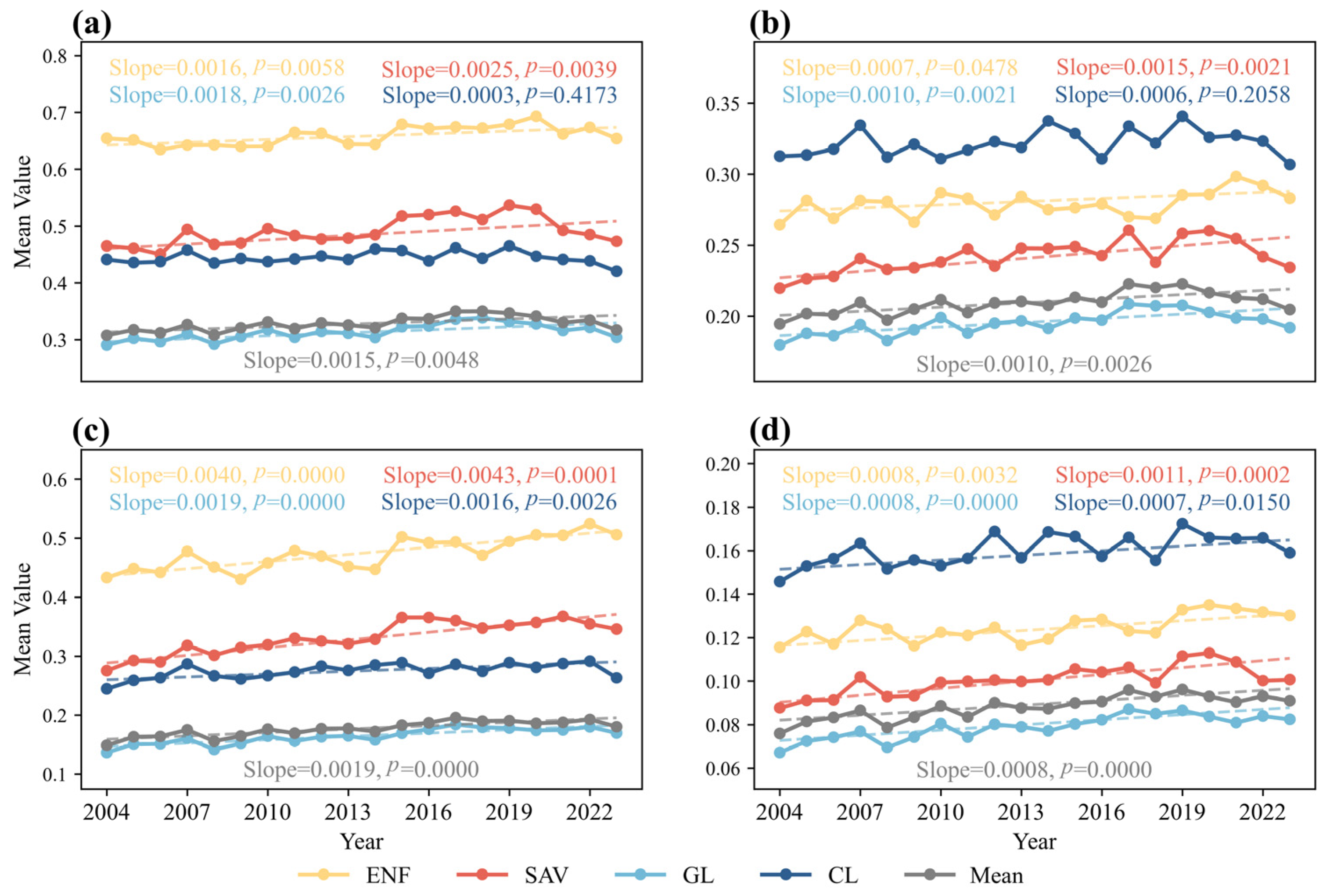
Based on the interannual mean variation in VIs during the growing season (April to October), the vegetation condition in the HRB has significantly improved over the past two decades (Figure 3). All four VIs exhibited significant upward trends (p < 0.05), with an average slope of 0.0013/yr. Among different vegetation types, savannas showed the highest average increase in VIs during the growing season, reaching 0.0024/yr, while croplands exhibited the lowest growth rate, at 0.0008/yr. Evergreen needleleaf forests consistently exhibited higher values in NDVI and kNDVI, while croplands showed the highest values in EVI and NIRv. Among the indices, kNDVI demonstrated the strongest increasing trend (0.0019/yr) during the growing season, followed by NDVI, while NIRv showed the weakest upward trend. In terms of overall robustness, kNDVI not only exhibited the highest slope but also the lowest relative uncertainty (68.2%), indicating more stable trend detection (Supplementary Table S3). By contrast, NDVI and EVI showed relatively higher overall uncertainties (>100%), while NIRv had moderate uncertainty (79.9%). Overall, VIs in the HRB displayed a fluctuating yet increasing trend during the growing season from 2004 to 2023.

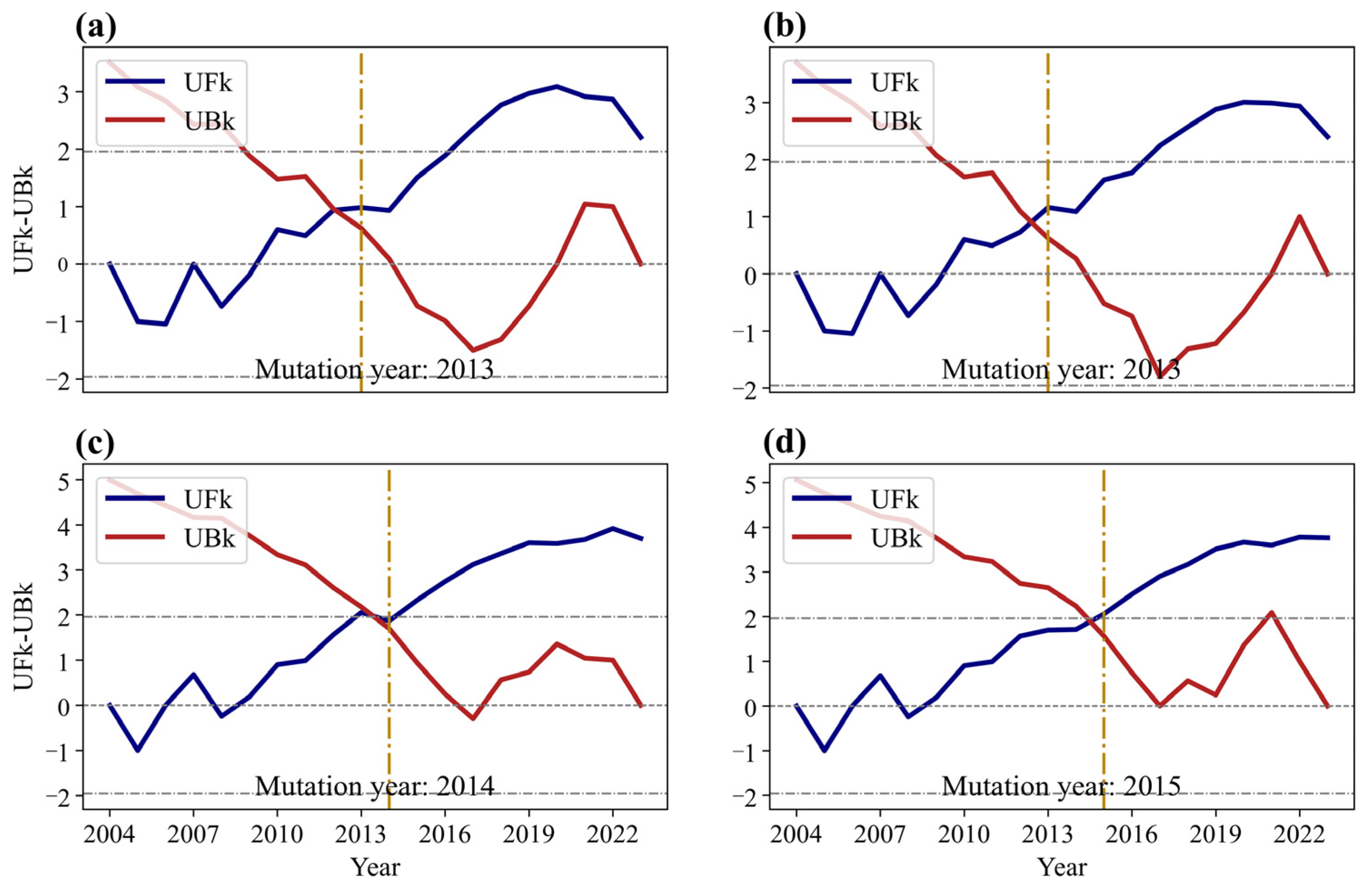
Despite long-term greening trends, vegetation growth in the HRB has exhibited a significant slowdown since the mid-2010s. Based on the M-K abrupt change test, changing points in the time series of VIs were identified: 2013 for NDVI and EVI, 2014 for kNDVI, and 2015 for NIRv, all corresponding to the intersection points of the UF and UB curves (Figure 4). To further analyze the vegetation change before and after the identified mutation years, we conducted a trend analysis for the two respective periods. The results showed that, prior to these mutation years (2004–2012), the average growth rate of the four VIs was 0.0016/yr (p < 0.05), whereas, in the post-mutation period, the growth rate significantly declined to 0.0002/yr (p > 0.05).

3.2. Spatial Variation Characteristics of Vegetation

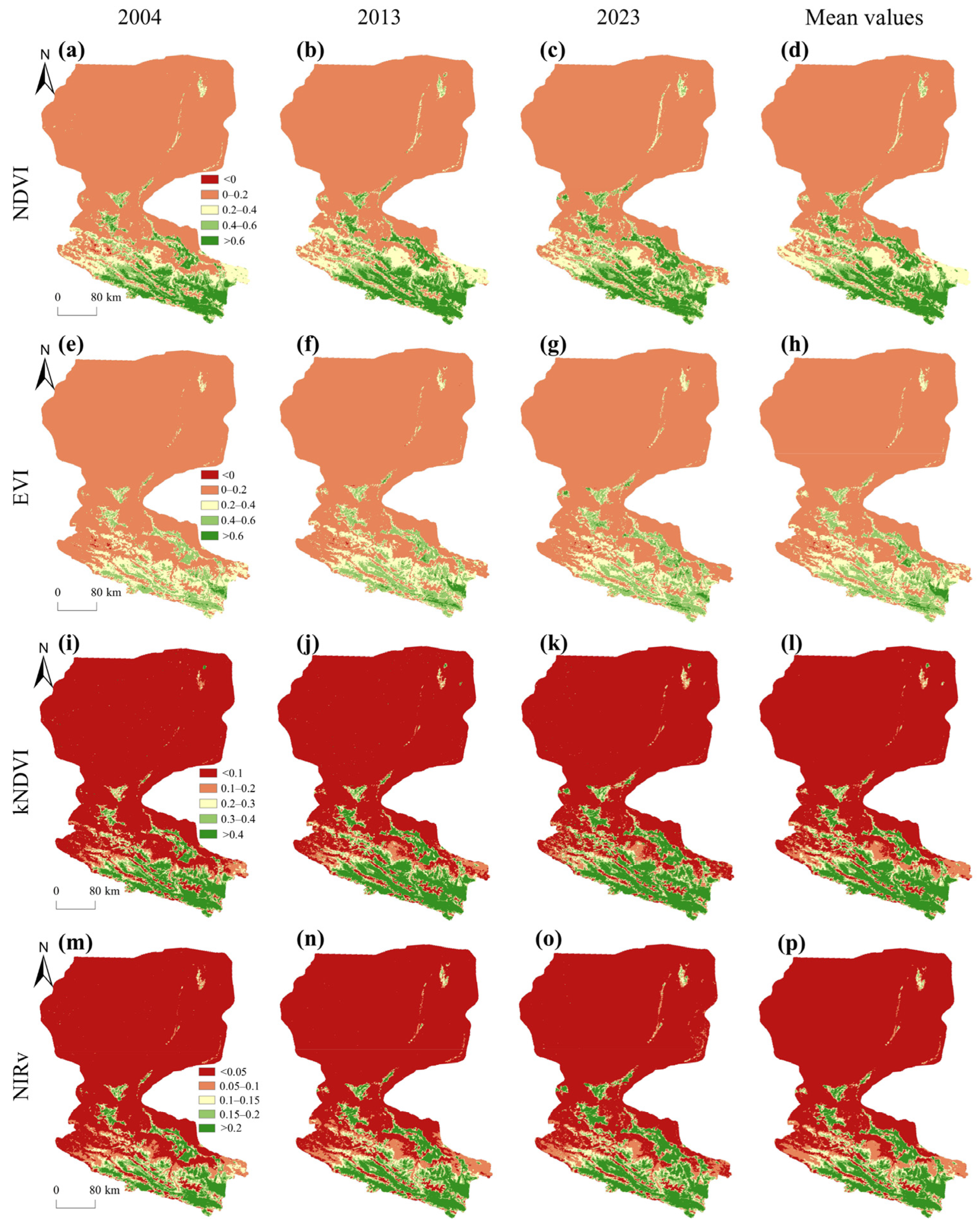
The long-term spatial evolution of vegetation in the HRB reveals a clear trend of improvement. From the spatial distribution map of the average VI in the HRB from 2004 to 2023 (Figure 5), a clear spatial variation is observed across all VIs. Regardless of the different VIs used, the overall distribution patterns remain consistent. With lower values predominantly found in the northern part of the study area, while higher values are mainly concentrated in the south. Moreover, all VIs exhibit a gradual decrease from southeast to northwest. A comparison of the spatial distribution of the four VIs reveals a notable improvement in vegetation coverage over time. Taking EVI as an example (Figure 5e–h), the area where the index exceeds 0.4 expanded from 11,361 km² in 2004 to 16,375 km² in 2013, and further to 16,815 km² in 2023 (

Table 6. Changes in vegetation area from 2004 to 2023.

VIs	Values	Area (km2)
		2004	2013	2023
NDVI	>0.4	24,491	29,076	28,571
EVI	>0.4	11,361	16,375	16,815
kNDVI	>0.3	18,942	24,441	26,035
NIRv	>0.15	17,731	22,593	24,105

). In addition, the increase in high-value areas was more pronounced for all VIs during the first decade (2004–2013) compared to the second decade (2013–2023). It suggests that vegetation growth in the region may be approaching a stabilization phase.

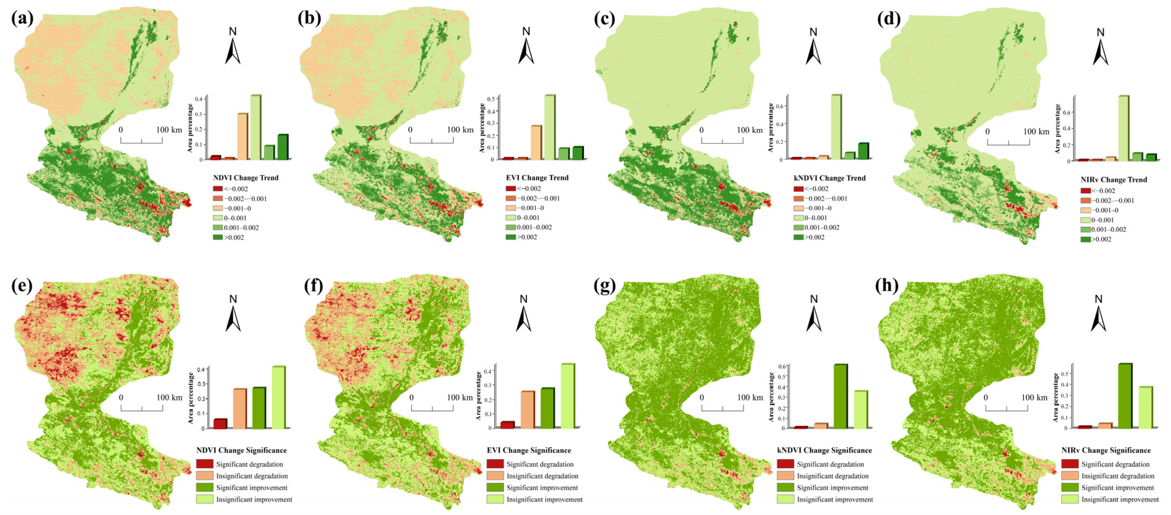
Furthermore, the pixel-by-pixel Theil–Sen slope and M-K test were conducted on the annual maximum composite VIs from 2004 to 2023 (Figure 6). From the trend maps, it can be observed that the spatial distribution of NDVI and EVI trends is generally similar. Regions with a slope greater than 0.001 account for 25.7% and 19.3% of the total area, respectively (Figure 6a,b), and are primarily located in the upper reaches of the HRB. Conversely, 2.8% and 2.6% of the area exhibit a slope lower than −0.001. For kNDVI and NIRv, the proportion of areas with a slope greater than 0.001 is 24.0% and 16.0% (Figure 6c,d), respectively, with the majority concentrated in the upper reaches of the basin. The proportion of areas with slope values between 0 and 0.001 is the highest for both indices, reaching approximately 70%, mainly distributed in the northern part of the basin, particularly in the southern region of the Inner Mongolia Plateau. Areas with negative slopes are relatively sparse and scattered.

Significant vegetation changes have occurred across a substantial portion of the HRB over the past two decades. The area that passed the M-K trend test accounts for 60.6% of the basin area, indicating widespread statistically significant trends. By integrating trend analysis with statistical significance testing results (Table 2), the spatial distribution of significant VI changes was obtained. Among the four VIs, significantly degraded areas account for 6.0%, 4.0%, 0.7%, and 0.7%, respectively (Figure 6e–h). These declining regions are primarily concentrated in urban centers, such as Zhangye City, Jiuquan City, and Yongchang County, Minle County, Jinta County, Gaotai County, Shandan County and Qilian County. In contrast, significantly improved areas account for 27.0%, 26.9%, 60.0%, and 58.4%, respectively, and are predominantly distributed north of the Qilian Mountains in the middle reaches of the basin and the Alxa Plateau region in the lower reaches.

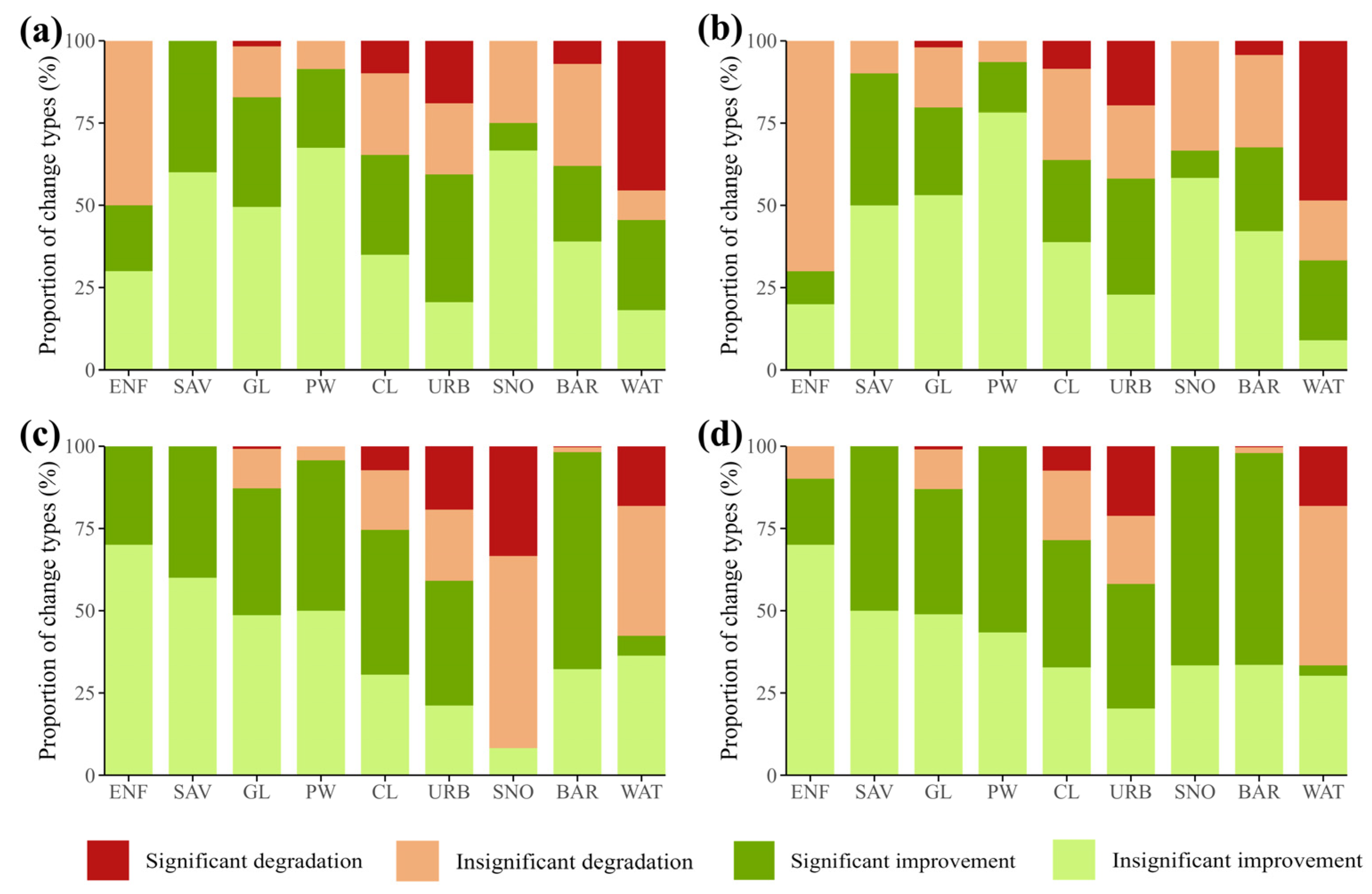
Figure 7 illustrates the proportions of vegetation change types across different land cover classes based on four VIs. Overall, SAV, GL, and PW were mainly improved, with the proportion of significant improvement generally exceeding 15%. Notably, kNDVI and NIRv showed significant improvement rates above 35%, and the total improvement exceeded 75% across all indices. In contrast, degradation was generally shown in human-disturbed or non-vegetation-dominated areas, such as CL, URB, SNO, and WAT. For instance, the proportion of significant degradation in water bodies exceeded 45% according to NDVI and EVI. In CL and URB, all VIs indicated over 25% degradation. It suggests that vegetation in natural land cover types has generally improved, whereas land cover types more strongly affected by human activities face a higher risk of degradation. Among the four indices, NIRv exhibited the lowest proportion of significant degradation (generally below 10% across most land cover types) and the highest proportion of improvement, indicating its greater stability and robustness in monitoring functional vegetation changes.

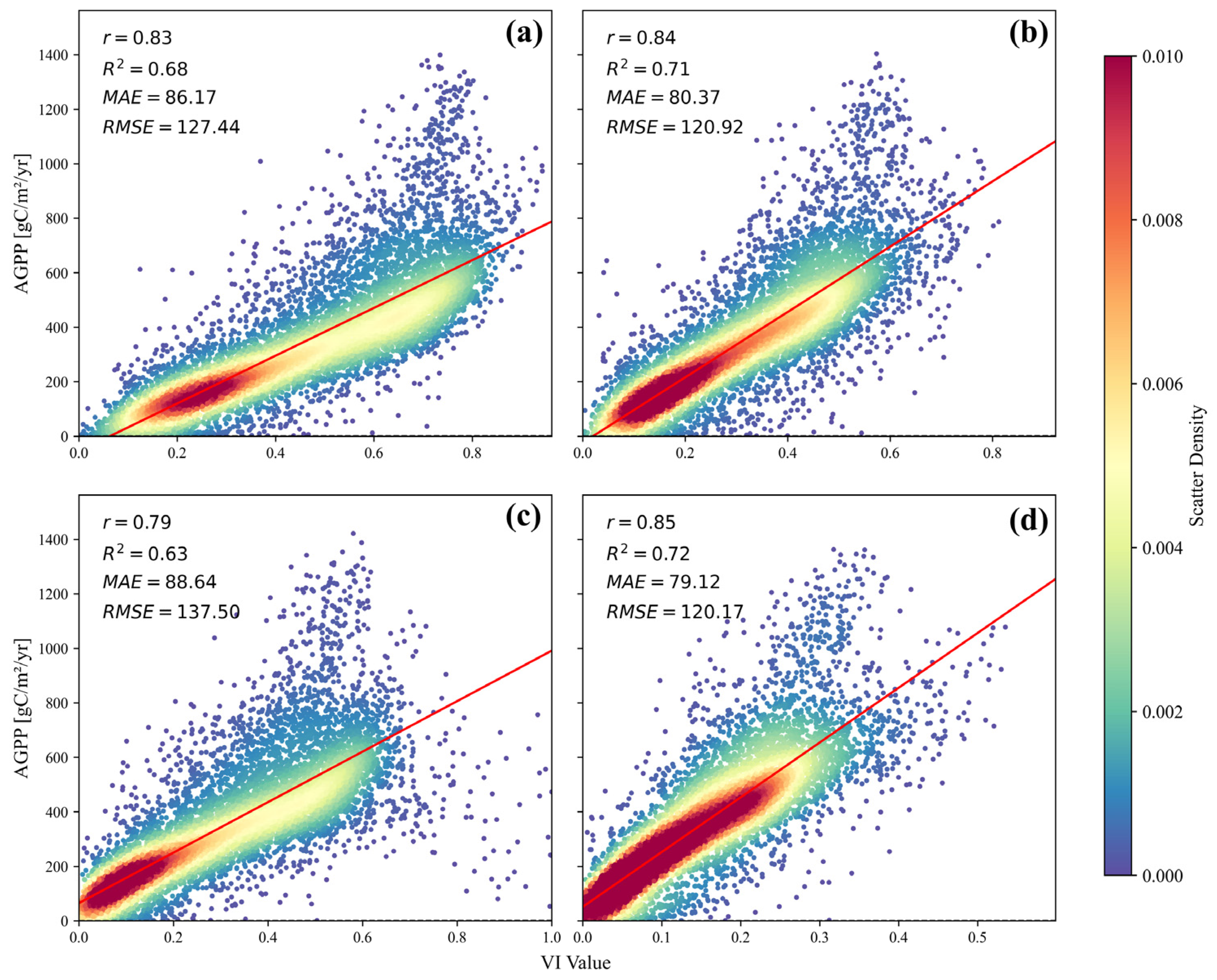
Figure 8 presents scatter plots illustrating the regression relationships between VIs and AGPP, along with model evaluation metrics. The results reveal strong positive correlations between all VIs and AGPP (p < 0.001), with correlation coefficients ranging from 0.79 for kNDVI to 0.85 for NIRv. Model accuracy assessments indicate that both NIRv and EVI demonstrated superior and comparable performance, significantly outperforming NDVI and kNDVI. Although the differences between NIRv and EVI were marginal, NIRv consistently exhibited slightly better metrics, achieving the highest R² of 0.72, the lowest RMSE of 120.17 gC/m²/yr, and the lowest MAE of 79.12 gC/m²/yr. Therefore, we selected NIRv as the representative proxy for the subsequent attribution analysis of vegetation dynamics in the HRB.

3.3. Driving Mechanisms of Vegetation Change

3.3.1. Impacts of Climatic and Non-Climatic Factors on Vegetation Change

Across the HRB, the average partial correlation coefficient between NIRv and precipitation is 0.18, while that between NIRv and temperature is 0.06. Regions where NIRv–precipitation correlations passed the t-test (p < 0.05), covering 6.3% of the basin and 3.8% exceeding a partial correlation coefficient of 0.6, mainly occurred north of the Qilian Mountains in the southern basin, the Beishan region, and a small portion of the northern Alxa Plateau (Supplementary Figure S1a). Significant partial correlations between NIRv and temperature covered 13.6% of the basin and 1.2% exceeding 0.6, mainly distributed in the central basin and along the downstream riparian zones of the Heihe River (Supplementary Figure S1b). Overall, annual maximum NIRv responded positively to both precipitation and temperature, with precipitation exerting a stronger influence on vegetation growth.

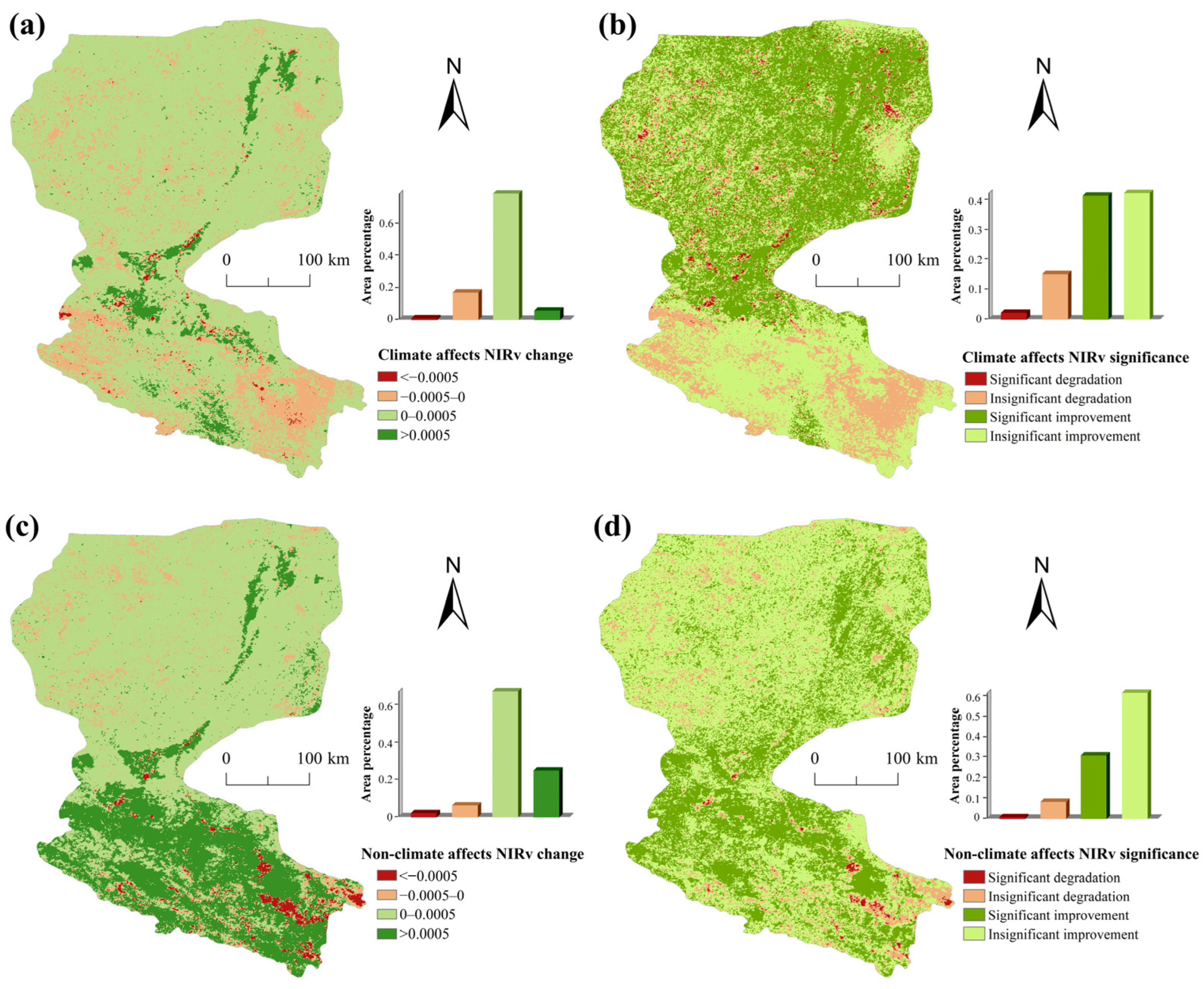
To identify the impact of climate change on vegetation, we performed multiple regression to simulate annual NIRv series driven by temperature and precipitation, based on which trend analysis was conducted. Vegetation across 82% of the HRB exhibited an increasing trend from 2004 to 2023 based on the Theil–Sen trend analysis (Figure 9a). Among these areas, regions with a slope greater than 0.0005 accounted for 5.1% of the basin, mainly located in the southern part of Jinta County and the Suzhou District within the central HRB, the upper eastern slopes of the Qilian Mountains, and the downstream riparian corridors of the Heihe River. Moreover, the M-K significance test identified that regions with statistically significant vegetation improvement were concentrated in the central HRB and the Alxa Plateau (Figure 9b), covering 40.9% of the total basin area. In contrast, only 2.1% of the basin showed significant vegetation degradation attributable to climatic factors. These findings suggest that climate change played a generally positive role in promoting vegetation growth in the HRB, particularly in its central and northern regions.

To quantify the impact of non-climatic factors on vegetation growth at the pixel scale, this study employed residual trend analysis to isolate the effects of non-climatic factors on NIRv dynamics in the HRB. Figure 9c, d present the Theil–Sen trend analysis and M-K significance test results for NIRv after removing climate influences through multiple regression residuals analysis. The study revealed that non-climatic factors facilitated vegetation enhancement across 66.6% of the HRB, with 27.5% of these areas exhibiting a slope greater than 0.0005. These zones predominantly occur in the central and southern subregions of the basin, as well as along the lower reaches of the Heihe River (Figure 9c). In contrast, vegetation degradation linked to non-climatic factors covered only 8.3% of the basin, with areas showing a slope less than −0.0005 accounting for merely 1.8%. Significant improvements in vegetation, attributed to non-climatic influence, spanned 30.6% of the basin (Figure 9d), primarily concentrated in the midstream and upstream reaches of the Heihe River, including the downstream alluvial fans of tributaries such as the Beida River. Conversely, areas exhibiting significant degradation comprised only 0.4%, largely clustered around administrative centers with high-intensity human activity, including Zhangye City, Jiuquan City, Yongchang County, Minle County, Jinta County, Gaotai County and Shandan County. These results indicate that, over the past two decades, non-climatic factors have predominantly promoted vegetation recovery across the HRB.

3.3.2. Contributions of Climatic and Non-Climatic Factors to Vegetation Change

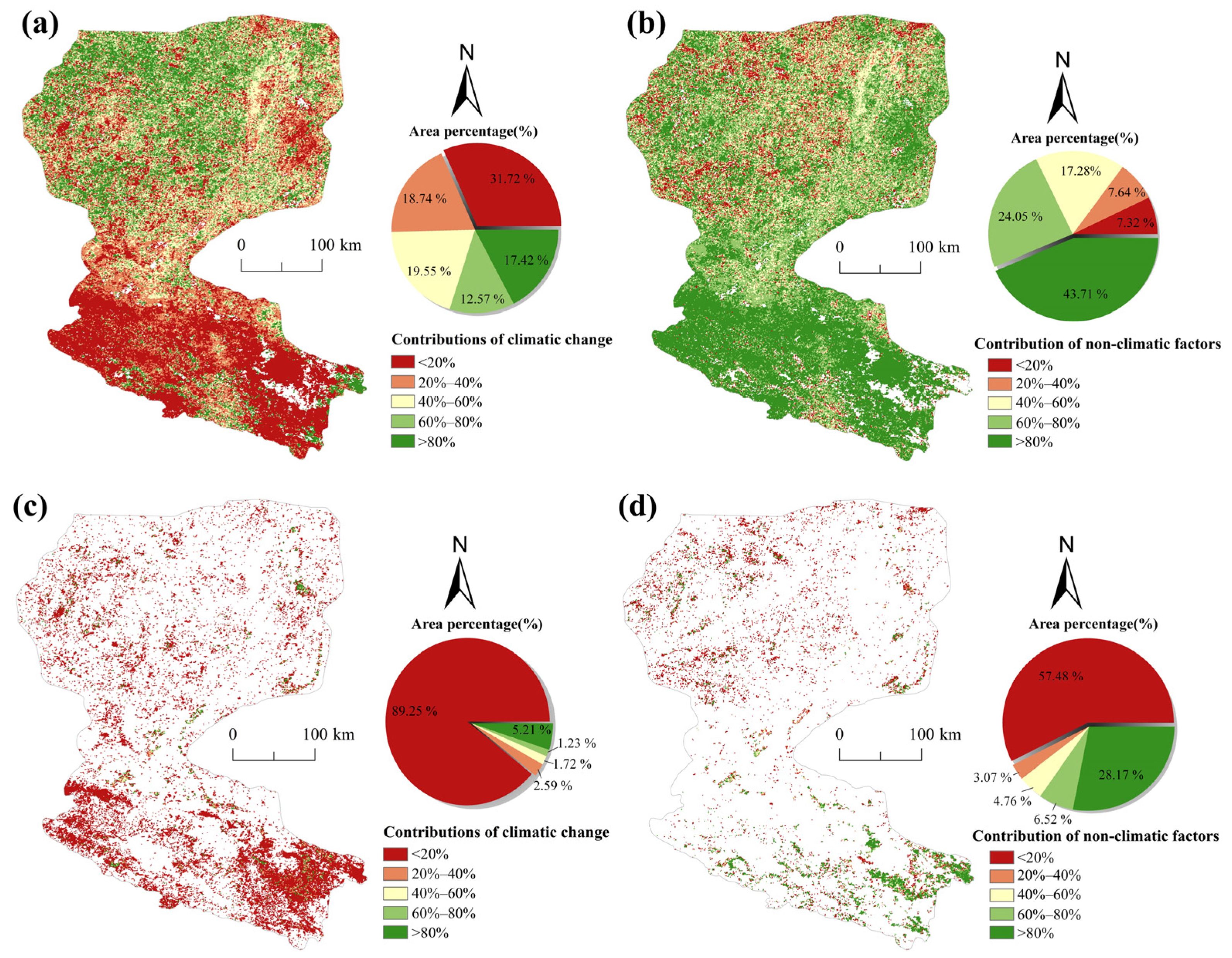
Areas with improved vegetation growth in the HRB cover 94.9% of the basin, a trend driven by both climate change and non-climatic factors. Among these, regions where non-climatic factors contribute over 80.0% to vegetation improvement make up 43.7%. These are primarily concentrated in the southern part of the basin, where urban settlements are densely distributed, as well as in the southeastern part of Ejin Banner (Figure 10b). In contrast, areas where climate change serves as the dominant driver (contribution rate > 80%) account for 17.4%, mostly found in the western Alxa Plateau in the northern HRB and a small portion of the southern Beishan Mountains (Figure 10a). Vegetation degradation influenced by both non-climatic factors and climate change affects 5.1% of the basin area. Among these, 28.2% of the degraded regions mainly result from non-climatic factors (contribution rate > 80%), concentrated in Zhangye City, Yongchang County, Minle County, and southern pastoral areas of Shandan County (Figure 10d). Regions where climate change drives over 80% of vegetation degradation cover just 5.2%, scattered along riparian zones (Figure 10c). Considering the spatial heterogeneity of the NIRv slope, we used the absolute slope of observed NIRv as a weight and calculated the weighted mean contribution of climate change and non-climatic factors. To evaluate the robustness of these estimates, we performed a bootstrap uncertainty analysis (1000 iterations). The results demonstrated that the relative contribution of climatic and non-climatic factors to vegetation change was 24% (95% CI: 23.8–24.1%) and 76% (95% CI: 75.9–76.2%), respectively.

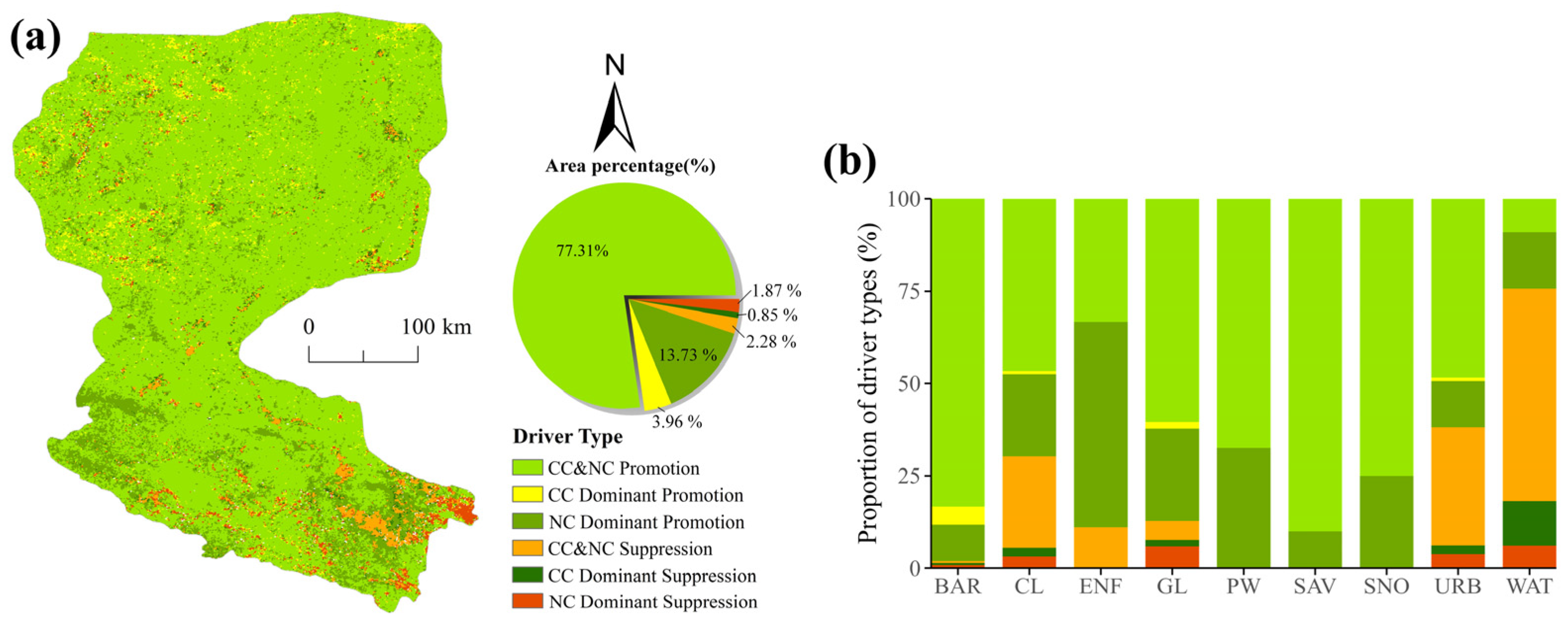
According to the spatial distribution of driving types (Figure 11a), areas where both climate and non-climate jointly promote vegetation growth account for the largest proportion, 77.3% of the entire basin. Climate-dominated improvement zones constitute 4.0%, while non-climate-dominated zones account for 13.7%, mainly located in suburban or rural areas. Regions where both drivers jointly suppress vegetation growth account for 2.3% of the basin, mainly concentrated in urban areas such as Zhangye, Minle, Jinta, Gaotai, and Ejina. Climate-dominated degradation accounts for 0.9% of the basin, while human-dominated degradation covers 1.9%, mainly distributed in Yongchang and Qilian counties. To further explore the potential impacts of climate change and non-climatic factors on NIRv, we calculated their relative contributions across different land cover types shown in Figure 11b. The result suggests that vegetation degradation or improvement region dominated by climate factors accounts for a relatively small proportion across all land cover types. For example, climate-dominant improvement occurs in only 1.80% of grasslands, while climate-dominant degradation is seen in just 2.2% of croplands. In contrast, regions where both climate and non-climate jointly promote NIRv increases dominate in barren lands, grasslands, permanent wetlands, savannas, and snow/ice-covered areas, each with a proportion exceeding 50%. The non-climatic factor of dominant vegetation improvement is most prominent in evergreen needleleaf forests (55.5%), grasslands (25.1%), and permanent wetlands (32.6%). Areas where both climate and non-climate jointly lead to NIRv degradation are mainly found in croplands (24.8%), urban and built-up lands (32.1%), and water bodies (57.6%). In comparison, vegetation degradation driven by non-climatic factors is relatively rare across all land cover types, with the highest proportion observed in water bodies, at just 6.1% (Figure 11b).

3.3.3. Further Analysis of Non-Climatic Driving Factors

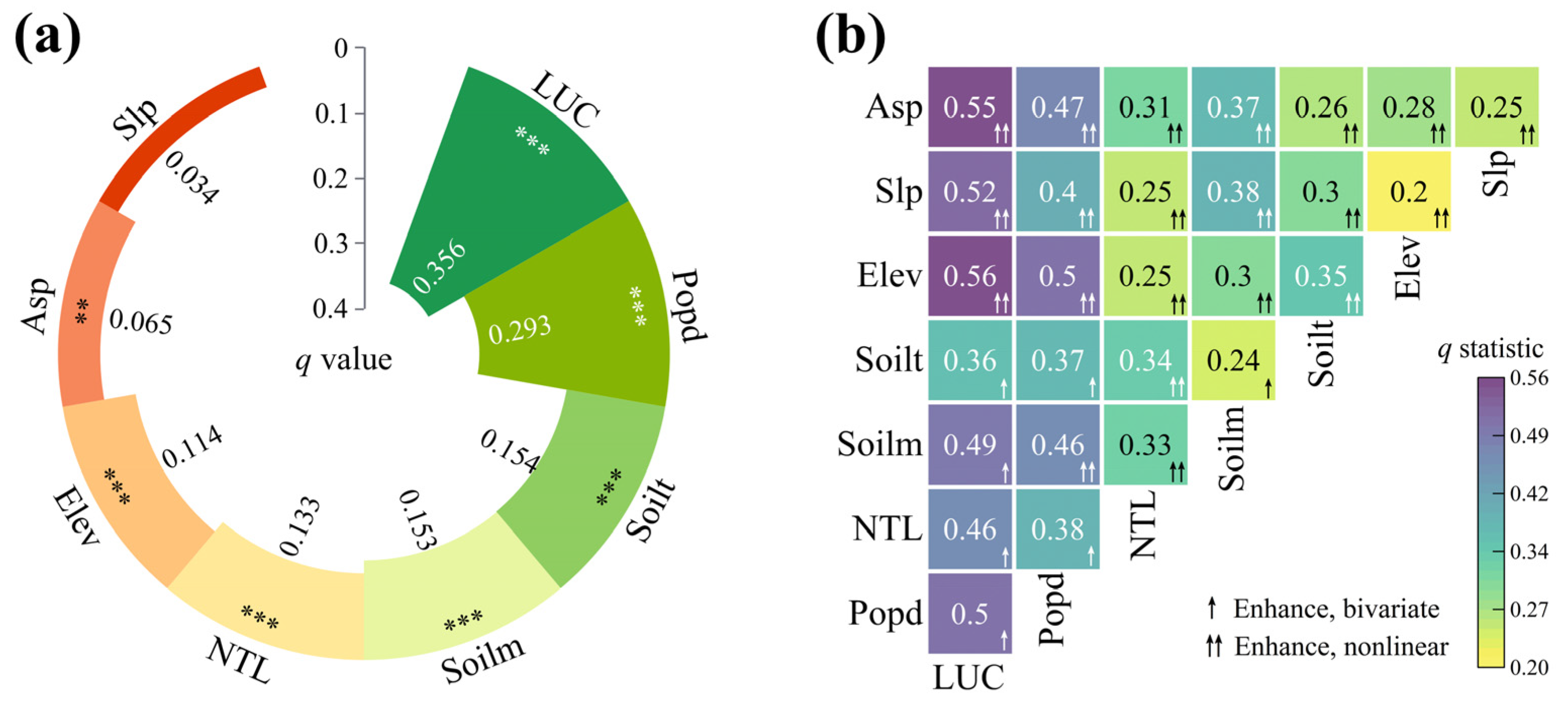
Given the dominant contribution of non-climatic factors (65%) to vegetation changes, we further utilized the OPGD model to dissect the internal components driving the residual NIRv trends. The factor detection results indicate that land use change (q = 0.356) and population density (q = 0.293) are the most influential factors affecting the NIRv residual trend, both significant at the 0.001 level, suggesting that human activities, represented by land use change and population density in this study, are the core non-climatic drivers of NIRv changes. In addition, soil texture (q = 0.154) and soil moisture (q = 0.153) show moderate explanatory power, indicating that surface physical properties still play a regulatory role in NIRv trends at the local scale. In contrast, topographic factors such as slope and aspect exhibit lower q-values, suggesting their direct influences on NIRv changes are limited (Figure 12a).

The interaction detection results revealed that, among the 28 pairs of variables, 7 exhibited bivariate enhancement and the remaining 21 showed nonlinear enhancement, indicating widespread synergistic effects among the factors (Figure 12b). The strongest interaction was observed between land use change and elevation (q = 0.56), followed by land use change and aspect (q = 0.55), and land use change and slope (q = 0.52), highlighting the significant role of land use interacting with topographic features in influencing the spatial heterogeneity of NIRv residual trends. In addition, interactions between population density and elevation (q = 0.50), as well as population density and soil moisture (q = 0.46), also demonstrated considerable explanatory power. Overall, the q-values of interaction terms were consistently higher than those of individual factors, underscoring the enhanced ability of compound drivers to explain non-climatic variations in NIRv.

Table 7. The results of ecological detector.

	LUC	Popd	NTL	Soilm	Soilt	Elev	Slp
Popd	Y
NTL	Y	Y
Soilm	Y	Y	Y
Soilt	Y	Y	Y	N
Elev	Y	Y	Y	Y	Y
Slp	Y	Y	Y	Y	Y	Y
Asp	Y	Y	Y	Y	Y	Y	Y

Note: Y denotes a significant difference between two factors, and N means no significant difference.

presents the differences in the spatiotemporal variation in NIRv explained by each pair of the eight selected factors. The results indicate that land use change, population density, nighttime lights, and topographic variables exhibit significant differences in their effects on NIRv compared to other factors, whereas soil moisture and soil texture show no statistically significant differences in their influence on the NIRv trend.

The risk detection results (

Table 8. Suitable type or range of different factors.

Factors	Suitable Type or Range	Mean NIRv Slope
Land use change	Unused land → Cropland	0.0109
Population density	10–24 person/km2	0.0044
Nighttime light	9–21 DN	0.0031
Soil moisture	0.255–0.301 m3/m3	0.0020
Soil texture	Loam	0.0019
Elevation	2480–2800 m	0.0030
Slope	0.634–0.981°	0.0016
Aspect	328–357°	0.0027

) show that regions with a land-use transition from unused land to cropland, population density of 10–24 persons/km², nighttime light intensity between 9 and 21, soil moisture of 0.255–0.301 m³/m³, and loam soil texture exhibit significantly higher NDVI slope values. These areas are generally located at elevations of 2480–2800 m, with gentle slopes (0.634–0.981°) and north slope (328–357°), suggesting that moderate human activity, favorable soil-water conditions, and topographic features jointly contribute to vegetation improvement in HRB.

4. Discussion

4.1. Spatiotemporal Variation Characteristics of Vegetation

The HRB exhibited a general greening trend from 2004 to 2023, with VIs increasing at a mean rate of 0.0013/yr with fluctuations (Figure 3), which aligns with findings by Han et al. (2023) [21] and Jiao et al. (2024) [68]. However, this overall trend conceals a significant biphasic pattern: a pronounced increase during 2004–2012 was followed by a significant slowdown in the rate of increase after a peak around 2017 (see Section 3.1). The initial rapid recovery is likely attributable to the marked effectiveness of large-scale ecological restoration projects, such as the EWDP, in their initial phase [21,48]. In contrast, the subsequent stabilization suggests that the ecosystems may be approaching a carrying capacity limited by regional water availability [69] or that the marginal benefits of restoration efforts are diminishing [70]. These findings imply that the era of rapid, project-driven greening may be plateauing, necessitating a strategic shift toward more nuanced and sustainable ecosystem management strategies in the region.

Across the four indices, evergreen needleleaf forests consistently exhibited higher values in NDVI and kNDVI, whereas croplands showed the highest values in EVI and NIRv (Figure 3). This pattern primarily arises because EVI minimizes soil background interference through blue-band correction, enhancing its sensitivity to rapid crop canopy dynamics [18], while NIRv effectively captures strong near-infrared scattering and high photosynthetic efficiency in agricultural canopies [19]. In contrast, dense evergreen forests are more prone to chlorophyll saturation effects [71], which are better detected by NDVI and kNDVI. Among the VIs, kNDVI demonstrated the strongest increasing trend during the growing season, followed by NDVI, whereas NIRv exhibited the weakest upward trend, indicating that kNDVI has higher sensitivity in capturing vegetation growth dynamics [72].

The trend of VIs changes exhibited significant spatial heterogeneity in the HRB. Vegetation degradation was mainly distributed in urban areas and their surroundings (Figure 6), which might be attributed to the rapid urbanization and land reclamation in the basin in recent decades [73]. The expansion of urban areas and croplands compresses the space available for vegetation growth, leading to vegetation degradation [74]. In contrast, significant vegetation improvement was observed in the northern slopes of the Qilian Mountains (upper reaches), irrigated croplands (middle reaches), and riparian zones of Ejina Banner (lower reaches), potentially driven by the ongoing implementation of policy measures such as upstream water conservation, midstream water-saving irrigation reform, and downstream ecological water replenishment [21,75].

4.2. Influences of Driving Factors on Vegetation Change

Non-climatic factors, predominantly human activities, have been the dominant driver (74%) of vegetation changes in the HRB, far exceeding the climatic contribution (26%). Among them, land use change was the most important non-climatic factor in explaining the residual trend of NIRv, which is consistent with the findings of Liu et al. (2021) [76]. Notably, despite the weak individual explanatory power of topographic variables, their interaction with land use change (q = 0.56) exhibited a strong synergistic effect, nonlinearly enhancing the explanatory power for vegetation change (Figure 12b). In the HRB, land use transformation primarily occurred in areas of low to moderate elevation (900–2500 m) [77]. This was especially evident in the middle reaches, where substantial conversions from unused land to grassland and from grassland to cropland were observed (Supplementary Figure S2), resulting in marked vegetation changes. In contrast, high-elevation regions such as the Qilian Mountains in the upper reaches are characterized by rugged terrain and limited accessibility, leading to fewer land use changes and correspondingly smaller variations in vegetation [78,79].

Driven by non-climatic factors, the improvement of vegetation in the midstream alluvial plain area is particularly significant, followed by the riparian zones at the downstream end (Figure 9c,d). However, the nature of this driver shows significant spatial variation. Vegetation improvement in the midstream alluvial plain is mainly related to land use changes. Our factor detection indicates that the conversion of unused land to cropland contributes the most to the NIRv increase (Table 8). This directly reflects the region’s development orientation as a core agricultural area [45]. However, this ‘greening’ growth essentially represents the expansion of artificial oases, which replace natural ecosystems. Its ecological value is different from that of natural vegetation and is highly dependent on irrigation water resources for maintenance [80]. This perpetuates the historical contradiction of ecological degradation downstream caused by the intensive water and soil resource development in the midstream [48]. The significant restoration of vegetation in the downstream riparian zones further confirms the effectiveness of the EWDP as a decisive policy intervention [49]. The EWDP ensures ecological water discharge, reconstructing hydrological connections in the downstream, thereby providing the necessary water conditions for the revival of natural vegetation, such as Populus euphratica [48]. This success profoundly highlights that the ecological crisis in the downstream is essentially a consequence of decades of high-intensity water and soil development in the midstream [48], and the EWDP serves as a forced correction to this historical imbalance. However, this also means that the health of the downstream ecosystem has shifted from relying on natural hydrological processes to relying on administratively allocated water resources, with its long-term stability deeply tied to water diversion policies [81]. Therefore, the sustainability of the basin cannot solely rely on “ecological transfusion” at the downstream; more efforts are needed in the midstream to fundamentally reconcile economic and ecological water use through improved water use efficiency [82] and optimized development models.

Among climatic factors, precipitation emerged as the dominant driver of vegetation change (see Section 3.3.1). This finding aligns with previous studies suggesting that water availability serves as the primary limiting factor for vegetation growth in arid and semi-arid regions, making vegetation more responsive to precipitation than to temperature or other climatic variables [83,84]. Areas with significant vegetation improvement mainly influenced by climatic factors are concentrated in the central and northern parts of the basin, particularly in the Alxa Plateau region (Figure 9b). This may be attributed to a recent increase in precipitation in this area [85], which has alleviated water limitations in the ecosystem and thus enhanced the potential for vegetation growth. In addition, studies have shown that rising temperatures have, to some extent, extended the growing season and improved photosynthetic efficiency, further promoting vegetation growth, especially in high-altitude and high-latitude regions [27,28].

Furthermore, the spatial distribution of driving types (Figure 11a) reveals that areas where climate and non-climate factors jointly promoted vegetation restoration accounted for the largest proportion (77.3%), suggesting that the combined effects of favorable climate and ecological restoration provided more advantageous conditions for vegetation improvement [86]. Although areas where climate and non-climate jointly suppressed vegetation growth only covered 2.3% of the basin (Figure 11b), they mainly clustered in densely populated and highly developed urban regions, revealing the vulnerability of ecosystems under strong disturbance [74]. In summary, non-climatic factors mainly drive vegetation change in the HRB and have greatly supported its recovery; however, greater ecological benefits are more likely when favorable climatic and environmental conditions combine with moderate human intervention.

4.3. Effectiveness, Limitations and Future Directions

This study integrates residual trend analysis and the OPGD, differing from traditional approaches that simply categorize driving forces into a binary structure of climate and human activities based solely on residuals. We not only initially separated climate and non-climate factors but also further refined the internal composition and complex interactions of non-climate drivers, thereby enhancing the understanding of natural–social coupled ecosystem dynamics. This method proves highly effective in identifying vegetation change mechanisms in arid regions. On one hand, residual trend analysis, through constructing a multivariate regression model between NIRv and climate variables, effectively isolates the impact of climatic factors on vegetation dynamics, allowing the residuals to more clearly represent the “pure effect” of non-climatic drivers, thereby improving the accuracy of identifying climatic and non-climatic contributions [37,38]. On the other hand, after obtaining the NIRv residual trend driven by non-climatic factors, the introduction of the OPGD method enables quantitative analysis of the explanatory power of various non-climatic drivers, such as land use change, population density, soil properties, and topographic features, on the residuals. Moreover, it detects nonlinear relationships and interactive effects among these factors [87,88], thus providing a more systematic and detailed understanding of the mechanisms behind non-climatic drivers. The results demonstrate that land use changes and ecological restoration projects played a crucial role in vegetation recovery in the HRB. These findings highlight the synergistic effects of natural and anthropogenic forces, offering insights for evaluating ecological project effectiveness and developing regional ecological management strategies.

However, this study still has several limitations, which call for further exploration in subsequent research. Firstly, although we applied trend analysis, significance testing, and abrupt change detection across four vegetation indices to comprehensively examine the spatiotemporal trends of vegetation in the HRB, seasonal vegetation dynamics and potential lagged responses to climate variables were not considered. Previous studies have indicated that climatic impacts on vegetation growth may exhibit significant lag effects and accumulation [25,89]. Secondly, this study’s reliance on a single vegetation index (NIRv) for attribution analysis presents a limitation. Although NIRv demonstrated marginally better performance, its advantage over other indices is minimal and context-dependent. Consequently, results may lack robustness across diverse biomes or conditions [90]. Future work should consider integrating multiple vegetation indices to enhance the generalizability of driver attribution. Thirdly, this study simplifies the selection of driving factors. The climate dimension mainly relies on precipitation and temperature, without incorporating key regulating factors such as potential evapotranspiration, solar radiation, and vapor pressure difference, which play crucial roles in vegetation growth in arid regions [69,91,92]. The non-climatic dimension also fails to fully consider other potential influencing factors, such as landform types and GDP [76,93]. The absence of these critical variables constrains our ability to develop a comprehensive understanding of the driving mechanisms behind vegetation dynamics. Finally, while combining residual analysis with OPGD refines the identification of non-climatic drivers, it inherently assumes that climatic and human influences are linearly separable, overlooking their complex interdependencies [94]. A key limitation is that climate variability directly influences human decisions (e.g., on water management, irrigation intensity, and land use), which in turn affect vegetation [95]. This creates feedback loops that our method cannot fully disentangle. Therefore, future studies should employ models capable of quantifying these feedbacks, such as structural equation modeling to elucidate causal pathways, or machine learning approaches to more comprehensively characterize the complex, non-linear compound effects of various driving factors [96].

5. Conclusions

This study quantifies spatiotemporal vegetation dynamics in the HRB (2004–2023) using a complementary multi-index validation approach and further investigates its underlying driving factors. Our results indicate that non-climatic factors, primarily land-use change and water management policies, are the dominant drivers of vegetation change in the HRB, accounting for 74% of the total variation in vegetation dynamics. In contrast, climatic factors, such as temperature and precipitation, only explain 26% of the observed changes. The interaction between land-use and elevation nonlinearly explained 56% of NIRv trends. Basin-wide greening occurred (+0.0013/yr) but slowed after 2013 (0.0002/yr) compared to the pre-2013 period (0.0011/yr). Degradation hotspots (3% coverage) clustered in urban centers, while significant improvement (43%) dominated the Qilian Mountains’ northern slopes, irrigated croplands, and Ejina riparian zones. Notably, while agricultural expansion has led to localized greening, it poses significant and well-documented risks to regional water security and long-term ecological stability. Based on these findings, it is essential to implement integrated management strategies that balance agricultural demands with the ecological water needs of the entire basin, ensuring long-term ecological stability and water security.

References

1. Bonan, G.B. Forests and Climate Change: Forcings, Feedbacks, and the Climate Benefits of Forests. Science 2008, 320, 1444–1449. [Google Scholar] [CrossRef] [PubMed]
2. Zhou, Z.; Ding, Y.; Shi, H.; Cai, H.; Fu, Q.; Liu, S.; Li, T. Analysis and Prediction of Vegetation Dynamic Changes in China: Past, Present and Future. Ecol. Indic. 2020, 117, 106642. [Google Scholar] [CrossRef]
3. Parmesan, C.; Yohe, G. A Globally Coherent Fingerprint of Climate Change Impacts across Natural Systems. Nature 2003, 421, 37–42. [Google Scholar] [CrossRef] [PubMed]
4. Zhou, Q.; Chen, W.; Wang, H.; Wang, D. Spatiotemporal Evolution and Driving Factors Analysis of Fractional Vegetation Coverage in the Arid Region of Northwest China. Sci. Total Environ. 2024, 954, 176271. [Google Scholar] [CrossRef] [PubMed]
5. Yin, D.; Li, X.; Huang, Y.; Si, Y.; Bai, R. Identifying Vegetation Dynamics and Sensitivities in Response to Water Resources Management in the Heihe River Basin in China. Adv. Meteorol. 2015, 2015, 861928. [Google Scholar] [CrossRef]
6. Liu, Q.; Cheng, P.; Lyu, M.; Yan, X.; Xiao, Q.; Li, X.; Wang, L.; Bao, L. Impacts of Climate Change on Runoff in the Heihe River Basin, China. Atmosphere 2024, 15, 516. [Google Scholar] [CrossRef]
7. Men, B.; Liu, H. Water Resource System Vulnerability Assessment of the Heihe River Basin Based on Pressure-State-Response (PSR) Model under the Changing Environment. Water Supply 2018, 18, 1956–1967. [Google Scholar] [CrossRef]
8. Huang, J.; Yu, H.; Guan, X.; Wang, G.; Guo, R. Accelerated Dryland Expansion under Climate Change. Nat. Clim. Change 2016, 6, 166–171. [Google Scholar] [CrossRef]
9. Smith, A.M.S.; Kolden, C.A.; Tinkham, W.T.; Talhelm, A.F.; Marshall, J.D.; Hudak, A.T.; Boschetti, L.; Falkowski, M.J.; Greenberg, J.A.; Anderson, J.W.; et al. Remote Sensing the Vulnerability of Vegetation in Natural Terrestrial Ecosystems. Remote Sens. Environ. 2014, 154, 322–337. [Google Scholar] [CrossRef]
10. Teng, Y.; Zhan, J.; Agyemang, F.B.; Sun, Y. The Effects of Degradation on Alpine Grassland Resilience: A Study Based on Meta-Analysis Data. Glob. Ecol. Conserv. 2020, 24, e01336. [Google Scholar] [CrossRef]
11. Hu, X.; Lu, L.; Li, X.; Wang, J.; Guo, M. Land Use/Cover Change in the Middle Reaches of the Heihe River Basin over 2000–2011 and Its Implications for Sustainable Water Resource Management. PLoS ONE 2015, 10, e0128960. [Google Scholar] [CrossRef]
12. Ren, Z.; Tian, Z.; Wei, H.; Liu, Y.; Yu, Y. Spatiotemporal Evolution and Driving Mechanisms of Vegetation in the Yellow River Basin, China during 2000–2020. Ecol. Indic. 2022, 138, 108832. [Google Scholar] [CrossRef]
13. Hilker, T.; Natsagdorj, E.; Waring, R.H.; Lyapustin, A.; Wang, Y. Satellite Observed Widespread Decline in Mongolian Grasslands Largely Due to Overgrazing. Glob. Change Biol. 2014, 20, 418–428. [Google Scholar] [CrossRef] [PubMed]
14. Liu, X.; Zhu, X.; Pan, Y.; Li, Y.; Zhao, A. Spatiotemporal Changes in Vegetation Coverage in China during 1982–2012. Acta Ecol. Sin. 2015, 35, 5331–5342. [Google Scholar]
15. Piao, S.; Fang, J. Dynamic vegetation cover change over the last 18 years in China. Quat. Sci. 2001, 21, 294–302. [Google Scholar]
16. Zhang, Y.; Song, C.; Band, L.E.; Sun, G.; Li, J. Reanalysis of Global Terrestrial Vegetation Trends from MODIS Products: Browning or Greening? Remote Sens. Environ. 2017, 191, 145–155. [Google Scholar] [CrossRef]
17. Fensholt, R.; Rasmussen, K.; Nielsen, T.T.; Mbow, C. Evaluation of Earth Observation Based Long Term Vegetation Trends—Intercomparing NDVI Time Series Trend Analysis Consistency of Sahel from AVHRR GIMMS, Terra MODIS and SPOT VGT Data. Remote Sens. Environ. 2009, 113, 1886–1898. [Google Scholar] [CrossRef]
18. Huete, A.R.; Liu, H.Q.; Batchily, K.; van Leeuwen, W. A Comparison of Vegetation Indices over a Global Set of TM Images for EOS-MODIS. Remote Sens. Environ. 1997, 59, 440–451. [Google Scholar] [CrossRef]
19. Badgley, G.; Field, C.B.; Berry, J.A. Canopy Near-Infrared Reflectance and Terrestrial Photosynthesis. Sci. Adv. 2017, 3, e1602244. [Google Scholar] [CrossRef]
20. Camps-Valls, G.; Campos-Taberner, M.; Moreno-Martínez, Á.; Walther, S.; Duveiller, G.; Cescatti, A.; Mahecha, M.D.; Muñoz-Marí, J.; García-Haro, F.J.; Guanter, L.; et al. A Unified Vegetation Index for Quantifying the Terrestrial Biosphere. Sci. Adv. 2021, 7, eabc7447. [Google Scholar] [CrossRef]
21. Han, Z.; Meng, J.; Zou, Y.; Zhu, L. Dynamics of Vegetation Index and Its Response to Climate Change and Ecological Construction Projects in Heihe River Basin from 1982 to 2017. J. Desert Res. 2023, 43, 96–106. [Google Scholar]
22. Tan, M.; Ran, Y.; Su, Y.; Li, X.; Du, D.; Lian, Y. Characteristics and Sustainability Evaluation of Vegetation Change in Heihe River Basin during 2001 to 2017. Remote Sens. Technol. Appl. 2020, 35, 335–344. [Google Scholar]
23. Huete, A.; Didan, K.; Miura, T.; Rodriguez, E.P.; Gao, X.; Ferreira, L.G. Overview of the Radiometric and Biophysical Performance of the MODIS Vegetation Indices. Remote Sens. Environ. 2002, 83, 195–213. [Google Scholar] [CrossRef]
24. Montandon, L.; Small, E. The Impact of Soil Reflectance on the Quantification of the Green Vegetation Fraction from NDVI. Remote Sens. Environ. 2008, 112, 1835–1845. [Google Scholar] [CrossRef]
25. Ding, Y.; Li, Z.; Peng, S. Global Analysis of Time-Lag and -Accumulation Effects of Climate on Vegetation Growth. Int. J. Appl. Earth Obs. Geoinf. 2020, 92, 102179. [Google Scholar] [CrossRef]
26. Fatima, Z.; Ahmed, M.; Hussain, M.; Abbas, G.; Ul-Allah, S.; Ahmad, S.; Ahmed, N.; Ali, M.A.; Sarwar, G.; Haque, E.U.; et al. The Fingerprints of Climate Warming on Cereal Crops Phenology and Adaptation Options. Sci. Rep. 2020, 10, 18013. [Google Scholar] [CrossRef]
27. Piao, S.; Yin, G.; Tan, J.; Cheng, L.; Huang, M.; Li, Y.; Liu, R.; Mao, J.; Myneni, R.B.; Peng, S.; et al. Detection and Attribution of Vegetation Greening Trend in China over the Last 30 Years. Glob. Change Biol. 2015, 21, 1601–1609. [Google Scholar] [CrossRef]
28. Zhong, L.; Ma, Y.; Salama, M.S.; Su, Z. Assessment of Vegetation Dynamics and Their Response to Variations in Precipitation and Temperature in the Tibetan Plateau. Clim. Change 2010, 103, 519–535. [Google Scholar] [CrossRef]
29. Zewdie, W.; Csaplovics, E.; Inostroza, L. Monitoring Ecosystem Dynamics in Northwestern Ethiopia Using NDVI and Climate Variables to Assess Long Term Trends in Dryland Vegetation Variability. Appl. Geogr. 2017, 79, 167–178. [Google Scholar] [CrossRef]
30. Huang, X.; An, R.; Wang, H.; Xing, F.; Wang, B.; Fan, M.; Fang, Y.; Lu, H. Differential Effects of Climatic and Non-Climatic Factors on the Distribution of Vegetation Phenology Trends on the Tibetan Plateau. Heliyon 2023, 9, e21069. [Google Scholar] [CrossRef]
31. Liang, T.; Tian, F.; Zou, L.; Jin, H.; Tagesson, T.; Rumpf, S.; He, T.; Liang, S.; Fensholt, R. Global Assessment of Vegetation Patterns along Topographic Gradients. Int. J. Digit. Earth 2024, 17, 2404232. [Google Scholar] [CrossRef]
32. Wei, Y.; Lu, H.; Wang, J.; Wang, X.; Sun, J. Dual Influence of Climate Change and Anthropogenic Activities on the Spatiotemporal Vegetation Dynamics over the Qinghai-Tibetan Plateau from 1981 to 2015. Earth’s Future 2022, 10, e2021EF002566. [Google Scholar] [CrossRef]
33. Jiang, L.; Jiapaer, G.; Bao, A.; Guo, H.; Ndayisaba, F. Vegetation Dynamics and Responses to Climate Change and Human Activities in Central Asia. Sci. Total Environ. 2017, 599–600, 967–980. [Google Scholar] [CrossRef] [PubMed]
34. Sun, Y.; Yang, Y.; Zhang, L.; Wang, Z. The Relative Roles of Climate Variations and Human Activities in Vegetation Change in North China. Phys. Chem. Earth Parts A/B/C 2015, 87–88, 67–78. [Google Scholar] [CrossRef]
35. Qi, G.; She, D.; Xia, J.; Song, J.; Jiao, W.; Li, J.; Liu, Z. Soil Moisture Plays an Increasingly Important Role in Constraining Vegetation Productivity in China over the Past Two Decades. Agric. For. Meteorol. 2024, 356, 110193. [Google Scholar] [CrossRef]
36. Zhu, Z.; Piao, S.; Myneni, R.B.; Huang, M.; Zeng, Z.; Canadell, J.G.; Ciais, P.; Sitch, S.; Friedlingstein, P.; Arneth, A.; et al. Greening of the Earth and Its Drivers. Nat. Clim. Change 2016, 6, 791–795. [Google Scholar] [CrossRef]
37. Jiang, X.; Fang, X.; Zhu, Q.; Jin, J.; Ren, L.; Jiang, S.; Yan, Y.; Yuan, S.; Liao, M. Time-Series Satellite Images Reveal Abrupt Changes in Vegetation Dynamics and Possible Determinants in the Yellow River Basin. Agric. For. Meteorol. 2024, 355, 110124. [Google Scholar] [CrossRef]
38. Qu, S.; Wang, L.; Lin, A.; Yu, D.; Yuan, M.; Li, C. Distinguishing the Impacts of Climate Change and Anthropogenic Factors on Vegetation Dynamics in the Yangtze River Basin, China. Ecol. Indic. 2020, 108, 105724. [Google Scholar] [CrossRef]
39. Chen, S.; Guo, B.; Zhang, R.; Zang, W.; Wei, C.; Wu, H.; Yang, X.; Zhen, X.; Li, X.; Zhang, D.; et al. Quantitatively Determine the Dominant Driving Factors of the Spatial—Temporal Changes of Vegetation NPP in the Hengduan Mountain Area during 2000–2015. J. Mt. Sci. 2021, 18, 427–445. [Google Scholar] [CrossRef]
40. Deng, X.; Hu, S.; Zhan, C. Attribution of Vegetation Coverage Change to Climate Change and Human Activities Based on the Geographic Detectors in the Yellow River Basin, China. Environ. Sci. Pollut. Res. 2022, 29, 44693–44708. [Google Scholar] [CrossRef]
41. Li, Z.; Yang, Q.; Ma, Z.; Chen, L.; Zhang, L. Responses of Vegetation to Climate Change and Human Activities in the Arid and Semiarid Regions of Northern China. Chin. J. Atmos. Sci. 2024, 48, 859–874. [Google Scholar] [CrossRef]
42. Song, Y.; Wang, J.; Ge, Y.; Xu, C. An Optimal Parameters-Based Geographical Detector Model Enhances Geographic Characteristics of Explanatory Variables for Spatial Heterogeneity Analysis: Cases with Different Types of Spatial Data. GISci. Remote Sens. 2020, 57, 593–610. [Google Scholar] [CrossRef]
43. Chen, Z.; Feng, H.; Liu, X.; Wang, H.; Hao, C. Analysis of the Influence of Driving Factors on Vegetation Changes Based on the Optimal-Parameter-Based Geographical Detector Model in the Yima Mining Area. Forests 2024, 15, 1573. [Google Scholar] [CrossRef]
44. Zhao, X.; Tan, S.; Li, Y.; Wu, H.; Wu, R. Quantitative Analysis of Fractional Vegetation Cover in Southern Sichuan Urban Agglomeration Using Optimal Parameter Geographic Detector Model, China. Ecol. Indic. 2024, 158, 111529. [Google Scholar] [CrossRef]
45. Liu, S.; Li, X.; Xu, Z.; Che, T.; Xiao, Q.; Ma, M.; Liu, Q.; Jin, R.; Guo, J.; Wang, L.; et al. The Heihe Integrated Observatory Network: A Basin-Scale Land Surface Processes Observatory in China. Vadose Zone J. 2018, 17, 1–21. [Google Scholar] [CrossRef]
46. Wang, Y.; Pan, J. Building Ecological Security Patterns Based on Ecosystem Services Value Reconstruction in an Arid Inland Basin: A Case Study in Ganzhou District, NW China. J. Clean. Prod. 2019, 241, 118337. [Google Scholar] [CrossRef]
47. Zhang, A.; Zheng, C.; Wang, S.; Yao, Y. Analysis of Streamflow Variations in the Heihe River Basin, Northwest China: Trends, Abrupt Changes, Driving Factors and Ecological Influences. J. Hydrol. Reg. Stud. 2015, 3, 106–124. [Google Scholar] [CrossRef]
48. Cheng, G.; Li, X.; Zhao, W.; Xu, Z.; Feng, Q.; Xiao, S.; Xiao, H. Integrated Study of the Water–Ecosystem–Economy in the Heihe River Basin. Natl. Sci. Rev. 2014, 1, 413–428. [Google Scholar] [CrossRef]
49. Lu, Z.; Feng, Q.; Xiao, S.; Xie, J.; Zou, S.; Yang, Q.; Si, J. The Impacts of the Ecological Water Diversion Project on the Ecology Hydrology-Economy Nexus in the Lower Reaches in an Inland River Basin. Resour. Conserv. Recycl. 2021, 164, 105154. [Google Scholar] [CrossRef]
50. Li, Y.; Cao, Z.; Long, H.; Liu, Y.; Li, W. Dynamic Analysis of Ecological Environment Combined with Land Cover and NDVI Changes and Implications for Sustainable Urban–Rural Development: The Case of Mu Us Sandy Land, China. J. Clean. Prod. 2017, 142, 697–715. [Google Scholar] [CrossRef]
51. Cai, Y.; Huang, W.; Teng, F.; Wang, B.; Ni, K.; Zheng, C. Spatial Variations of River–Groundwater Interactions from Upstream Mountain to Midstream Oasis and Downstream Desert in Heihe River Basin, China. Hydrol. Res. 2016, 47, 501–520. [Google Scholar] [CrossRef]
52. Strahler, A.H.; Muller, J.; Lucht, W.; Schaaf, C.; Tsang, T.; Gao, F.; Li, X.; Lewis, P.; Barnsley, M.J. MODIS BRDF/Albedo Product: Algorithm Theoretical Basis Document Version 5.0. Available online: https://modis.gsfc.nasa.gov/data/atbd/atbd_mod09.pdf (accessed on 22 August 2024).
53. Sellers, P.J.; Berry, J.A.; Collatz, G.J.; Field, C.B.; Hall, F.G. Canopy Reflectance, Photosynthesis, and Transpiration. III. A Reanalysis Using Improved Leaf Models and a New Canopy Integration Scheme. Remote Sens. Environ. 1992, 42, 187–216. [Google Scholar] [CrossRef]
54. Gu, Z.; Duan, X.; Shi, Y.; Li, Y.; Pan, X. Spatiotemporal Variation in Vegetation Coverage and Its Response to Climatic Factors in the Red River Basin, China. Ecol. Indic. 2018, 93, 54–64. [Google Scholar] [CrossRef]
55. Friedl, M.A.; Sulla-Menashe, D.; Tan, B.; Schneider, A.; Ramankutty, N.; Sibley, A.; Huang, X. MODIS Collection 5 Global Land Cover: Algorithm Refinements and Characterization of New Datasets. Remote Sens. Environ. 2010, 114, 168–182. [Google Scholar] [CrossRef]
56. Ning, J.; Liu, J.; Kuang, W.; Xu, X.; Zhang, S.; Yan, C.; Li, R.; Wu, S.; Hu, Y.; Du, G.; et al. Spatiotemporal Patterns and Characteristics of Land-Use Change in China during 2010–2015. J. Geogr. Sci. 2018, 28, 547–562. [Google Scholar] [CrossRef]
57. Fan, R.; Zhu, X.; Chen, Z.; Yu, G.; Zhang, W.; Han, L.; Wang, Q.; Chen, S.; Liu, S.; Wang, H.; et al. A dataset of annual gross primary productivity over Chinese terrestrial ecosystems during 2000–2020. China Sci. Data 2023, 8, 1–20. [Google Scholar]
58. Zhang, Y.; Kong, D.; Gan, R.; Chiew, F.H.S.; McVicar, T.R.; Zhang, Q.; Yang, Y. Coupled Estimation of 500 m and 8-Day Resolution Global Evapotranspiration and Gross Primary Production in 2002–2017. Remote Sens. Environ. 2019, 222, 165–182. [Google Scholar] [CrossRef]
59. Peng, S.; Ding, Y.; Liu, W.; Li, Z. 1 Km Monthly Temperature and Precipitation Dataset for China from 1901 to 2017. Earth Syst. Sci. Data 2019, 11, 1931–1946. [Google Scholar] [CrossRef]
60. Farr, T.G.; Rosen, P.A.; Caro, E.; Crippen, R.; Duren, R.; Hensley, S.; Kobrick, M.; Paller, M.; Rodriguez, E.; Roth, L.; et al. The Shuttle Radar Topography Mission. Rev. Geophys. 2007, 45, RG2004. [Google Scholar] [CrossRef]
61. Wu, Y.; Shi, K.; Chen, Z.; Liu, S.; Chang, Z. An Improved Time-Series DMSP-OLS-like Data (1992–2024) in China by Integrating DMSP-OLS and SNPP-VIIRS 2021. Harvard Dataverse, V7. Available online: https://dataverse.harvard.edu/dataset.xhtml?persistentId=doi:10.7910/DVN/GIYGJU (accessed on 27 August 2024).
62. Yang, Y.; Wang, S.; Bai, X.; Tan, Q.; Li, Q.; Wu, L.; Tian, S.; Hu, Z.; Li, C.; Deng, Y. Factors Affecting Long-Term Trends in Global NDVI. Forests 2019, 10, 372. [Google Scholar] [CrossRef]
63. Neeti, N.; Eastman, J.R. A Contextual Mann-Kendall Approach for the Assessment of Trend Significance in Image Time Series. Trans. GIS 2011, 15, 599–611. [Google Scholar] [CrossRef]
64. Liu, Z.; Wang, H.; Li, N.; Zhu, J.; Pan, Z.; Qin, F. Spatial and Temporal Characteristics and Driving Forces of Vegetation Changes in the Huaihe River Basin from 2003 to 2018. Sustainability 2020, 12, 2198. [Google Scholar] [CrossRef]
65. Zhong, R.; Wang, P.; Mao, G.; Chen, A.; Liu, J. Spatiotemporal Variation of Enhanced Vegetation Index in the Amazon Basin and Its Response to Climate Change. Phys. Chem. Earth Parts A/B/C 2021, 123, 103024. [Google Scholar] [CrossRef]
66. Nordberg, M.-L.; Evertson, J. Vegetation Index Differencing and Linear Regression for Change Detection in a Swedish Mountain Range Using Landsat TM® and ETM+® Imagery. Land Degrad. Dev. 2005, 16, 139–149. [Google Scholar] [CrossRef]
67. Zhong, X.; Wu, R. Analysis of Changing Trends in NDVI and Their Driving Forces in the Tuojiang River Basin Based on Animproved BFAST Model. Remote Sens. Nat. Resour. 2025, 37, 131–141. [Google Scholar]
68. Jiao, D.; Liu, S.; Xu, Z.; Song, L.; Li, Y.; Liu, R.; Wei, J.; He, X.; Wu, D.; Xu, T.; et al. Spatio-Temporal Variations and Multi-Scale Correlations of Climate, Water, Land, and Vegetation Resources over the Past Four Decades in the Heihe River Basin. J. Hydrol. Reg. Stud. 2024, 55, 101941. [Google Scholar] [CrossRef]
69. Liu, J.; Cao, W.; Yuan, Y.; Li, S.; Wang, P. Interannual Variations in Water Budget and Vegetation Coverage Dynamics in Desert Ecosystems of Heihe River Basin. Water 2025, 17, 2660. [Google Scholar] [CrossRef]
70. Zhou, T.; Akiyama, T.; Horita, M.; Kharrazi, A.; Kraines, S.; Li, J.; Yoshikawa, K. The Impact of Ecological Restoration Projects in Dry Lands: Data-Based Assessment and Human Perceptions in the Lower Reaches of Heihe River Basin, China. Sustainability 2018, 10, 1471. [Google Scholar] [CrossRef]
71. Zeng, Y.; Hao, D.; Park, T.; Zhu, P.; Huete, A.; Myneni, R.; Knyazikhin, Y.; Qi, J.; Nemani, R.R.; Li, F.; et al. Structural Complexity Biases Vegetation Greenness Measures. Nat. Ecol. Evol. 2023, 7, 1790–1798. [Google Scholar] [CrossRef]
72. Wang, Q.; Moreno-Martínez, Á.; Muñoz-Marí, J.; Campos-Taberner, M.; Camps-Valls, G. Estimation of Vegetation Traits with Kernel NDVI. ISPRS J. Photogramm. Remote Sens. 2023, 195, 408–417. [Google Scholar] [CrossRef]
73. Wang, S.; Ge, Y. Ecological Quality Response to Multi-Scenario Land-Use Changes in the Heihe River Basin. Sustainability 2022, 14, 2716. [Google Scholar] [CrossRef]
74. Zhang, L.; Yang, L.; Zohner, C.M.; Crowther, T.W.; Li, M.; Shen, F.; Guo, M.; Qin, J.; Yao, L.; Zhou, C. Direct and Indirect Impacts of Urbanization on Vegetation Growth across the World’s Cities. Sci. Adv. 2022, 8, eabo0095. [Google Scholar] [CrossRef]
75. Wang, P.; Wang, Y.; Han, X.; Han, H.; Zhang, D.; Zhang, P. Dynamic Changes of Vegetation Coverage in Heihe River Basin from 1990 to 2019 and the Effect of Temperature on It. Geol. Surv. China 2021, 8, 64–71. [Google Scholar] [CrossRef]
76. Liu, C.; Li, W.; Wang, W.; Zhou, H.; Liang, T.; Hou, F.; Xu, J.; Xue, P. Quantitative Spatial Analysis of Vegetation Dynamics and Potential Driving Factors in a Typical Alpine Region on the Northeastern Tibetan Plateau Using the Google Earth Engine. CATENA 2021, 206, 105500. [Google Scholar] [CrossRef]
77. Meng, J.; Cheng, H.; Li, F.; Han, Z.; Wei, C.; Wu, Y.; You, N.W.; Zhu, L. Spatial-Temporal Trade-Offs of Land Multi-Functionality and Function Zoning at Finer Township Scale in the Middle Reaches of the Heihe River. Land Use Policy 2022, 115, 106019. [Google Scholar] [CrossRef]
78. Jiang, Y.; Du, W.; Chen, J.; Wang, C.; Wang, J.; Sun, W.; Chai, X.; Ma, L.; Xu, Z. Climatic and Topographical Effects on the Spatiotemporal Variations of Vegetation in Hexi Corridor, Northwestern China. Diversity 2022, 14, 370. [Google Scholar] [CrossRef]
79. Wu, L.; Yang, Y.; Yang, H.; Xie, B.; Luo, W. A Comparative Study on Land Use/Land Cover Change and Topographic Gradient Effect between Mountains and Flatlands of Southwest China. Land 2023, 12, 1242. [Google Scholar] [CrossRef]
80. Du, J.; Fu, B.; Guo, Q.; Shi, P. Monitoring and Assessment of the Oasis Ecological Resilience Improved by Rational Water Dispatching Using Multiple Remote Sensing Data: A Case Study of the Heihe River Basin, Silk Road. Remote Sens. 2020, 12, 2577. [Google Scholar] [CrossRef]
81. Zhang, M.; Wang, S.; Fu, B.-J.; Gao, G.; Shen, Q. Ecological Effects and Potential Risks of the Water Diversion Project in the Heihe River Basin. Sci. Total Environ. 2017, 619–620, 794–803. [Google Scholar] [CrossRef]
82. Cai, W.; Jiang, X.; Sun, H.; Lei, Y.; Nie, T.; Li, L. Spatial Scale Effect of Irrigation Efficiency Paradox Based on Water Accounting Framework in Heihe River Basin, Northwest China. Agric. Water Manag. 2023, 277, 108118. [Google Scholar] [CrossRef]
83. Chen, H.; Ren, Z. Response of Vegetation Coverage to Changes of Precipitation and Temperature in Chinese Mainland. Bull. Soil Water Conserv. 2013, 33, 78–82+4. [Google Scholar] [CrossRef]
84. Liu, C.; Liu, B.; Zhao, W.; Zhu, Z. Temporal and Spatial Variability of Water Use Efficiency of Vegetation and Its Response to Precipitation and Temperature in Heihe River Basin. Acta Ecol. Sin. 2020, 40, 888–899. [Google Scholar] [CrossRef]
85. Wang, L.; Zhang, W.; Yu, Y.; Wang, D.; Zhao, Y.; Xie, X.; Chang, J. Characteristics and Differences of Climate Change in Shule River Basin and Heihe River Basin. Open J. Nat. Sci. 2023, 11, 125–138. [Google Scholar] [CrossRef]
86. Qiao, X.; Liu, P.; Ren, Y.; Si, W.; Hua, Y. Analysis of the Characteristics and Driving Factors of Ecological Environment Changes in Heihe River Basin Based on Remote Sensing Data. China Environ. Sci. 2020, 40, 3962–3971. [Google Scholar] [CrossRef]
87. Wang, Y.; Zhang, Z.; Chen, X. Quantifying Influences of Natural and Anthropogenic Factors on Vegetation Changes Based on Geodetector: A Case Study in the Poyang Lake Basin, China. Remote Sens. 2021, 13, 5081. [Google Scholar] [CrossRef]
88. Yang, S.; Zhao, Y.; Yang, D.; Lan, A. Analysis of Vegetation NDVI Changes and Driving Factors in the Karst Concentration Distribution Area of Asia. Forests 2024, 15, 398. [Google Scholar] [CrossRef]
89. Wen, Y.; Liu, X.; Pei, F.; Li, X.; Du, G. Non-Uniform Time-Lag Effects of Terrestrial Vegetation Responses to Asymmetric Warming. Agric. For. Meteorol. 2018, 252, 130–143. [Google Scholar] [CrossRef]
90. Wang, X.; Biederman, J.A.; Knowles, J.F.; Scott, R.L.; Turner, A.J.; Dannenberg, M.P.; Köhler, P.; Frankenberg, C.; Litvak, M.E.; Flerchinger, G.N.; et al. Satellite Solar-Induced Chlorophyll Fluorescence and near-Infrared Reflectance Capture Complementary Aspects of Dryland Vegetation Productivity Dynamics. Remote Sens. Environ. 2022, 270, 112858. [Google Scholar] [CrossRef]
91. Leng, S.; Huete, A.; Cleverly, J.; Gao, S.; Yu, Q.; Meng, X.; Qi, J.; Zhang, R.; Wang, Q. Assessing the Impact of Extreme Droughts on Dryland Vegetation by Multi-Satellite Solar-Induced Chlorophyll Fluorescence. Remote Sens. 2022, 14, 1581. [Google Scholar] [CrossRef]
92. Paciolla, N.; Corbari, C.; Hu, G.; Zheng, C.; Menenti, M.; Jia, L.; Mancini, M. Evapotranspiration Estimates from an Energy-Water-Balance Model Calibrated on Satellite Land Surface Temperature over the Heihe Basin. J. Arid Environ. 2021, 188, 104466. [Google Scholar] [CrossRef]
93. Nie, T.; Dong, G.; Jiang, X.; Lei, Y. Spatio-Temporal Changes and Driving Forces of Vegetation Coverage on the Loess Plateau of Northern Shaanxi. Remote Sens. 2021, 13, 613. [Google Scholar] [CrossRef]
94. Zhu, L.; Meng, J.; Zhu, L. Applying Geodetector to Disentangle the Contributions of Natural and Anthropogenic Factors to NDVI Variations in the Middle Reaches of the Heihe River Basin. Ecol. Indic. 2020, 117, 106545. [Google Scholar] [CrossRef]
95. He, X.; Liang, J.; Zeng, G.; Yuan, Y.; Li, X. The Effects of Interaction between Climate Change and Land-Use/Cover Change on Biodiversity-Related Ecosystem Services. Glob. Chall. 2019, 3, 1800095. [Google Scholar] [CrossRef]
96. Wang, N.; Shen, L.; Fei, W.; Liu, Y.; Zhao, H.; Liu, L.; Wang, A.; He, B.-J. Seasonal Effects of Urban Morphology on the Thermal Environment Based on Automated Machine Learning: A Case Study of Beijing. Remote Sens. 2025, 17, 3150. [Google Scholar] [CrossRef]
Figure 1. Location, elevation, land use and land cover, and administrative divisions of the HRB. (a) shows the location of the study area in China and its administrative divisions. (b) shows the elevation and river distribution within the study area. (c) represents land use and land cover classification, in which ENF denotes evergreen needleleaf forests, SAV represents savannas, GL refers to grasslands, PW indicates permanent wetlands, CL stands for croplands, URB represents urban and built-up lands, SNO refers to permanent snow and ice, BAR denotes barren lands, and WAT indicates water bodies.
Remotesensing 17 03496 g001
Figure 2. Flowchart of this study.
Remotesensing 17 03496 g002
Figure 3. Temporal variation characteristics of VIs under different vegetation types. (a) NDVI; (b) EVI; (c) kNDVI; (d) NIRv. Trend lines are displayed when p < 0.05 but not shown when p > 0.05. ENF denotes evergreen needleleaf forests, SAV represents savannas, GL refers to grasslands and CL stands for croplands.
Remotesensing 17 03496 g003
Figure 4. Mutation year detection in vegetation areas using different indices. (a) NDVI; (b) EVI; (c) kNDVI; (d) NIRv.
Remotesensing 17 03496 g004
Figure 5. Spatial distribution of annual maximum VIs in HRB. The rows represent different years, and the columns represent different VIs. (ad) NDVI in 2004, 2013, 2023, and the mean during 2004–2023; (eh) EVI, (il) kNDVI, and (mp) NIRv for the corresponding years.
Remotesensing 17 03496 g005
Figure 6. Spatial variation characteristics of various VIs in the HBR. Among them, (ad) represent the changing trends of VIs; (eh) represent the significance of the changes in VIs. The histograms denote the area percentage of different degrees of change trends and significance of changes.
Remotesensing 17 03496 g006
Figure 7. Proportion of different change types of VIs under different land use and land cover. (a) Proportion of different change types of NDVI under various land use and land cover types; (bd) same as (a) but for EVI, kNDVI, and NIRv, respectively.
Remotesensing 17 03496 g007
Figure 8. Scatter plot of fitting comparison between the four VIs and AGPP. (ad) represent the fitting relationships between NDVI, EVI, kNDVI, and NIRv with AGPP, respectively. The p-values are all less than 0.001. Each group randomly selects 10,000 data points for display. Among them, the units of both RMSE and MAE are gC/m2/yr.
Remotesensing 17 03496 g008
Figure 9. Impact of climatic and non-climatic factors on spatiotemporal changes in vegetation. (a,b) denote the changing trend and significant characteristics of NIRv under the influence of climatic factors, while (c,d) represent those under the influence of non-climatic factors. The bar graphs represent the proportion of each impact level in the basin area.
Remotesensing 17 03496 g009
Figure 10. Spatial distribution of the contributions of climatic and non-climatic factors to vegetation improvement and degradation in the HRB. (a,b) denote contributions to vegetation improvement. (c,d) denote contributions to vegetation degradation.
Remotesensing 17 03496 g010
Figure 11. Spatial distribution of driving types in the HRB. CC&NC indicates vegetation changes jointly driven by climate and non-climate, while CC and NC represent changes mainly driven by climate and non-climate, respectively. (a) represents the distribution and area percentage of each driving type. (b) represents the proportion of driving types under different LULC.
Remotesensing 17 03496 g011
Figure 12. Results of the OPGD. (a) shows the factor detection results, where “***” indicates p < 0.001 and “**” indicates p < 0.01. (b) presents the interaction detection results.
Remotesensing 17 03496 g012