Article

Prediction of Thermal Response of Burning Outdoor Vegetation Using UAS-Based Remote Sensing and Artificial Intelligence

by
Pirunthan Keerthinathan
1,*,
Imanthi Kalanika Subasinghe
2,
Thanirosan Krishnakumar
2,
Anthony Ariyanayagam
2,
Grant Hamilton
3 and
Felipe Gonzalez
1
1
QUT Centre for Robotics, School of Electrical Engineering and Robotics, Faculty of Engineering, Queensland University of Technology (QUT), 2 George Street, Brisbane City, QLD 4000, Australia
2
School of Civil and Environmental Engineering, Faculty of Engineering, Queensland University of Technology (QUT), Brisbane, QLD 4000, Australia
3
School of Biology and Environmental Science, Faculty of Science, Queensland University of Technology (QUT), Brisbane, QLD 4000, Australia
*
Author to whom correspondence should be addressed.
Remote Sens. 2025, 17(20), 3454; https://doi.org/10.3390/rs17203454
Submission received: 30 August 2025 / Revised: 8 October 2025 / Accepted: 14 October 2025 / Published: 16 October 2025

Abstract

Highlights

What are the main findings?
  • Developed a UAS-based framework to identify and delineate Lilly Pilly vegetation using ML, watershed, and point cloud delineation tool.
  • Built a predictive model estimating simulation-based Lilly Pilly vegetation thermal responses with >99% validation accuracy.
What are the implications of the main findings?
  • Demonstrate a scalable method to assess wildfire risk near residential areas.
  • Extendable to multiple species, varied vegetation shapes, and higher-altitude UAS imagery.

Abstract

The increasing frequency and intensity of wildfires pose severe risks to ecosystems, infrastructure, and human safety. In wildland–urban interface (WUI) areas, nearby vegetation strongly influences building ignition risk through flame contact and radiant heat exposure. However, limited research has leveraged Unmanned Aerial Systems (UAS) remote sensing (RS) to capture species-specific vegetation geometry and predict thermal responses during ignition events This study proposes a two-stage framework integrating UAS-based multispectral (MS) imagery, LiDAR data, and Fire Dynamics Simulator (FDS) modeling to estimate the maximum temperature (T) and heat flux (HF) of outdoor vegetation, focusing on Syzygium smithii (Lilly Pilly). The study data was collected at a plant nursery at Queensland, Australia. A total of 72 commercially available outdoor vegetation samples were classified into 11 classes based on pixel counts. In the first stage, ensemble learning and watershed segmentation were employed to segment target vegetation patches. Vegetation UAS-LiDAR point cloud delineation was performed using Raycloudtools, then projected onto a 2D raster to generate instance ID maps. The delineated point clouds associated with the target vegetation were filtered using georeferenced vegetation patches. In the second stage, cone-shaped synthetic models of Lilly Pilly were simulated in FDS, and the resulting data from the sensor grid placed near the vegetation in the simulation environment were used to train an XGBoost model to predict T and HF based on vegetation height (H) and crown diameter (D). The point cloud delineation successfully extracted all Lilly Pilly vegetation within the test region. The thermal response prediction model demonstrated high accuracy, achieving an RMSE of 0.0547 °C and R2 of 0.9971 for T, and an RMSE of 0.1372 kW/m2 with an R2 of 0.9933 for HF. This study demonstrates the framework’s feasibility using a single vegetation species under controlled ignition simulation conditions and establishes a scalable foundation for extending its applicability to diverse vegetation types and environmental conditions.

1. Introduction

Wildfires (also known as bushfires) represent a growing threat to biodiversity, infrastructure, and human lives, especially in climate-vulnerable regions such as Australia, southern Europe, and the western United States. Climate change has significantly intensified wildfire frequency, duration, and severity, driven by prolonged droughts, rising temperatures, and erratic weather patterns [1,2]. Vegetation plays a central role in fire propagation, acting as fuel that influences ignition, spread rate, intensity, and suppression difficulty [3]. As wildland–urban interface (WUI) regions expand, urban and peri-urban infrastructures such as residential buildings, power lines, water supply systems, and transportation corridors face escalating vulnerability to direct flame contact, radiant heat exposure, and firebrand attacks [4,5].
In wildfire science, accurately characterizing these thermal responses, through including surface temperature (T), radiative heat flux (HF), and convective heat transfer from vegetation to nearby structures, is essential for modeling ignition potential and predicting fire spread in the built environment [6,7]. These thermal parameters are critical for assessing the ignitability of building envelope components (e.g., siding, roofing materials) and determining their compliance with established radiant heat flux thresholds [8,9,10,11]. Thermal properties such as solid-phase density, Arrhenius reaction rate, mass yield of gas products, heat of reaction, and heat of combustion are critical vegetation-level indicators that influence fire behavior. However, most widely used wildfire behavior models, such as FARSITE, BehavePlus, PHOENIX RapidFire, FlamMap, simulate landscape-scale dynamics using generalized fuel models, and typically lack the granularity to simulate vegetation-level thermal outputs or localized heat transfer to buildings [12,13,14,15]. Table 1 presents a summary of key studies on estimating thermal and fire behavior parameters using remote sensing or experimentally acquired data. Uncrewed Aerial Systems (UAS) platforms equipped with Red Green and Blue (RGB), Multispectral (MS), Hyperspectral (HS) and close-range light detection and ranging (LiDAR) sensors can collect detailed information on vegetation structure, health, and composition [16,17]. LiDAR technology provides 3D point clouds that accurately capture canopy geometry, volume, height, and biomass distribution key parameters for fire behavior modeling and heat transfer simulations [18,19].
Despite the growing application of UAS-based RS in vegetation analysis [29,30,31,32], its use remains largely concentrated on invasive species monitoring and weed detection. HS and MS imagery has been widely used for deep learning models focused on species-level segmentation [33]. While MS imagery from UAS platforms has proven effective in segmenting vegetation types [34,35], its potential for classifying outdoor ornamental vegetations especially in the context of wildfire risk has been significantly underexplored. The accurate delineation of outdoor vegetation point clouds could enable direct integration into fire behavior simulation software [24], providing a non-destructive pathway for estimating thermal responses. However, no existing study has fully leveraged UAS-based RS to extract species-specific geometric details and predict their maximum thermal responses in the event of ignition. This research addresses this gap by developing a methodology that combines UAS-based RS and Artificial Intelligence (AI) to predict the thermal responses such as T and HF on building walls situated at different distances from outdoor vegetation.
The integration of LiDAR technology with computational modeling has emerged as an advancement in wildfire research, addressing the growing need for accurate prediction in the context of increasing wildfire frequency and intensity globally. Hendawitharana et al. [25] developed LiDAR-based Computational Fluid Dynamics (CFD) heat transfer models specifically designed for bushfire conditions, demonstrating how high-resolution point cloud data can be directly integrated into FDS to investigate wind velocities, temperature profiles, and pressure distributions during fire events. Liu et al. [36] advanced the field by integrating multi-source RS data for comprehensive forest fire risk assessment, combining satellite imagery with other geospatial datasets to create more robust predictive frameworks that enhance spatial and temporal resolution of fire risk mapping. The characterization of forest structure at the crown level has been further refined by Rocha et al. [26], utilized both airborne and terrestrial laser scanning to quantify crown-level structure and fuel load in longleaf pine ecosystems. Sakellariou et al. [27] presented an integrated wildfire risk assessment framework that combines simulation modeling with RS data fusion, applicable to both natural and anthropogenic ecosystems, highlighting the potential of hybrid approaches that leverage multiple data sources and modeling techniques. While these studies have made substantial contributions to fire risk assessment, structural characterization, and physics-based fire modeling, a critical gap remains in the rapid prediction of thermal responses. The necessity of the present research lies in developing a UAS-based framework that combines high-resolution RS with AI to rapidly predict fire-induced T and HF responses.
To address the outlined research gaps, this study aims to demonstrate the feasibility of a framework that estimates the thermal responses (T and HF) of burning outdoor vegetation using collected UAS data and Machine Learning (ML). The primary goal is to predict HF and T generated by vegetation such as Lilly Pilly (Syzygium smithii), a common ornamental species in Queensland, Australia [37]. Despite their popularity, the fire-related characteristics of this species remain under-investigated. Given its proximity to buildings and potential role in fire spread across residential zones, these species represent an example case for ornamental vegetation fire risk assessment. In this context we focus on Lilly Pilly, specifically its widespread use in residential gardens and hedges. The proposed methodology is structured around two core models:
  • Lilly Pilly semantic segmentation: This focuses on the segmentation of Lilly Pilly, using MS imagery captured by UAS. Training data was manually labeled from imagery collected at a large nursery site [38], and a stacked ensemble learning (EL) approach was employed to train the semantic segmentation model. The model’s performance was evaluated using standard metrics to assess its predictive accuracy and segmentation quality.
  • Thermal response prediction: This is developed to estimate the maximum T and HF that would result if the segmented vegetation were to ignite. Structural parameters were extracted from LiDAR point clouds to generate synthetic data of Lilly Pilly geometries across a range of sizes. The thermal responses of the Lilly Pilly were derived from Simultaneous Thermal Analyzer (STA) tests and incorporated into the simulation. The synthetic vegetation models were voxelized and used in Fire Dynamic Simulator (FDS) to simulate and determine the maximum values of thermal responses at varying distances using a grid of T and HF sensors. To address the high computational cost and scenario-specific setup of physics-based fire simulations, we employ a data-driven model that enables rapid thermal response prediction without the burden of full CFD computations.
By providing scientifically validated, species-specific thermal responses, this work offers a foundation for understanding the maximum thermal response of outdoor vegetations in the event of combustion. The framework developed herein establishes a methodological foundation for future interdisciplinary studies that incorporate vegetation physiology, combustion science, and AI in the context of fire-prone built environments.

2. Materials and Methods

2.1. Experimental Design

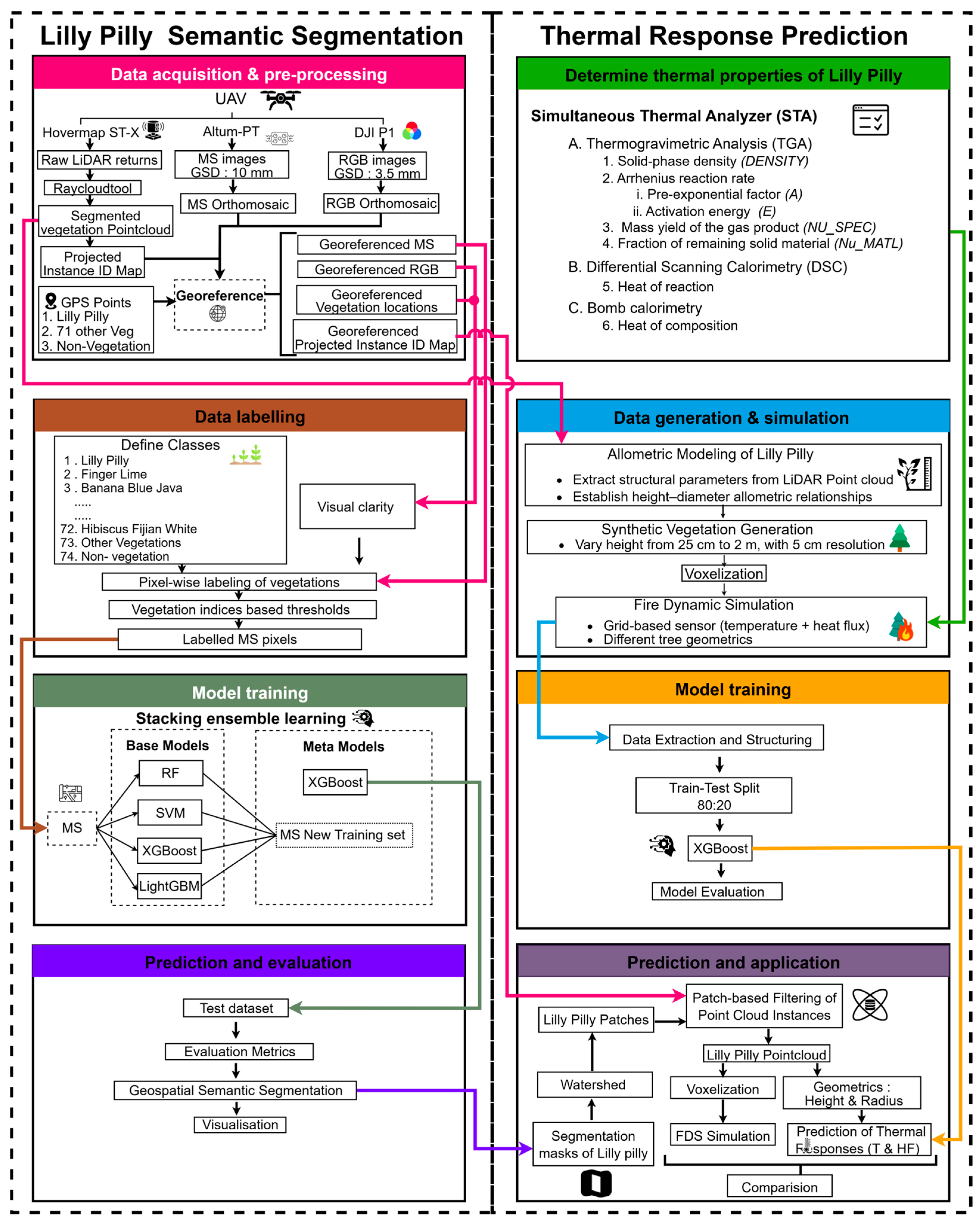
This study employs a two-stage framework to assess the risk of burning outdoor vegetations using RS and AI. The framework consists of: (1) Lilly Pilly semantic segmentation model, where the target species is classified from UAS-based MS imagery; and (2) Thermal response prediction model, where species-specific thermal outputs, including maximum value of T and HF, are predicted from the learnings of FDS. Figure 1 illustrates the workflow of the study that develops both models. The semantic segmentation model incorporates data acquisition, pre-processing, pixel-wise labeling, model training, and evaluation. The thermal response prediction model integrates laboratory experiments for the determination of thermal responses of Lilly Pilly, data generation for simulation, training the model using the simulated dataset, and subsequent prediction and evaluation.

2.2. Study Site

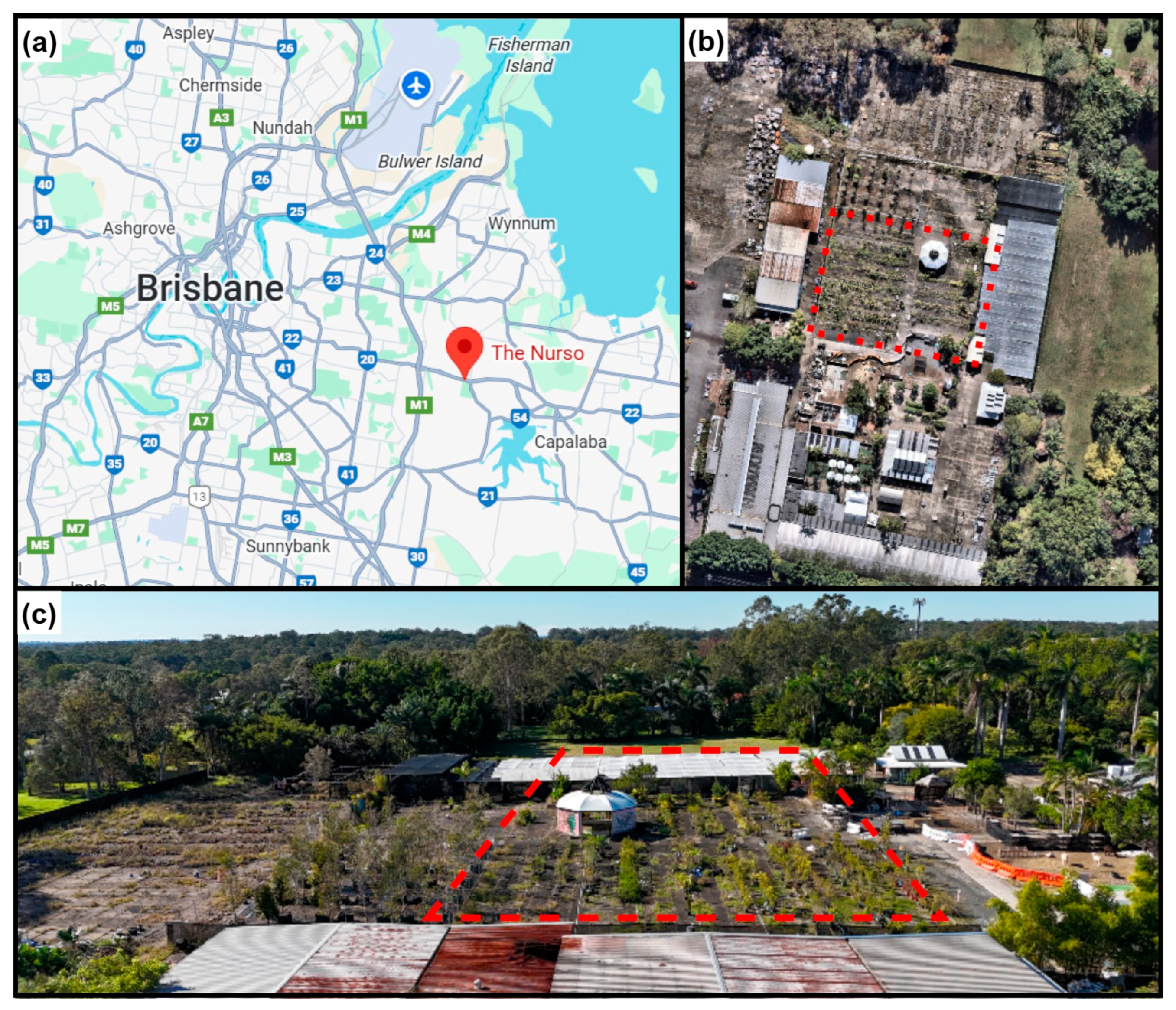
The study site, located at 1666 Old Cleveland Rd, Chandler, QLD 4153, Australia (27°30′26″S, 153°08′50″E) is relatively a low-lying region of southeastern Brisbane. The location of the selected site is approximately 15 km east of Brisbane city, providing a semi-urban environment suitable for assessing ornamental vegetation flammability. A high-resolution aerial map of the area, captured via UAS, is presented in Figure 2.
The selected location, the Nurso, is a commercial nursery spanning approximately 0.54 hectares, has a diverse collection of ornamental outdoor vegetations, including multiple varieties of Syzygium smithii, making it ideal for vegetation segmentation and species-specific analysis. The selected location’s terrain exhibits an average elevation of approximately 25–31 m above sea level, with minimal topographic variability making it predominantly flat with gentle undulations between 1 m and 153 m in localized terrain highs [39].

2.3. Data Acquisition

UAS-based data acquisition was carried out at noon on 12 June 2025, employing a multi-sensor approach to capture detailed spatial and spectral information of the site. The aerial campaign utilized several advanced sensors mounted on UAS, including the DJI Zenmuse P1 for high-resolution RGB imaging, the Micasense Altum-PT for MS data, and the Hovermap ST-X for LiDAR data collection. The Hovermap ST-X was also used in a handheld configuration to conduct complementary ground-level LiDAR scanning.
Figure 1. Overview of the study methodology, highlighting the key steps in developing the Lilly Pilly semantic segmentation and thermal response prediction model.
Remotesensing 17 03454 g001
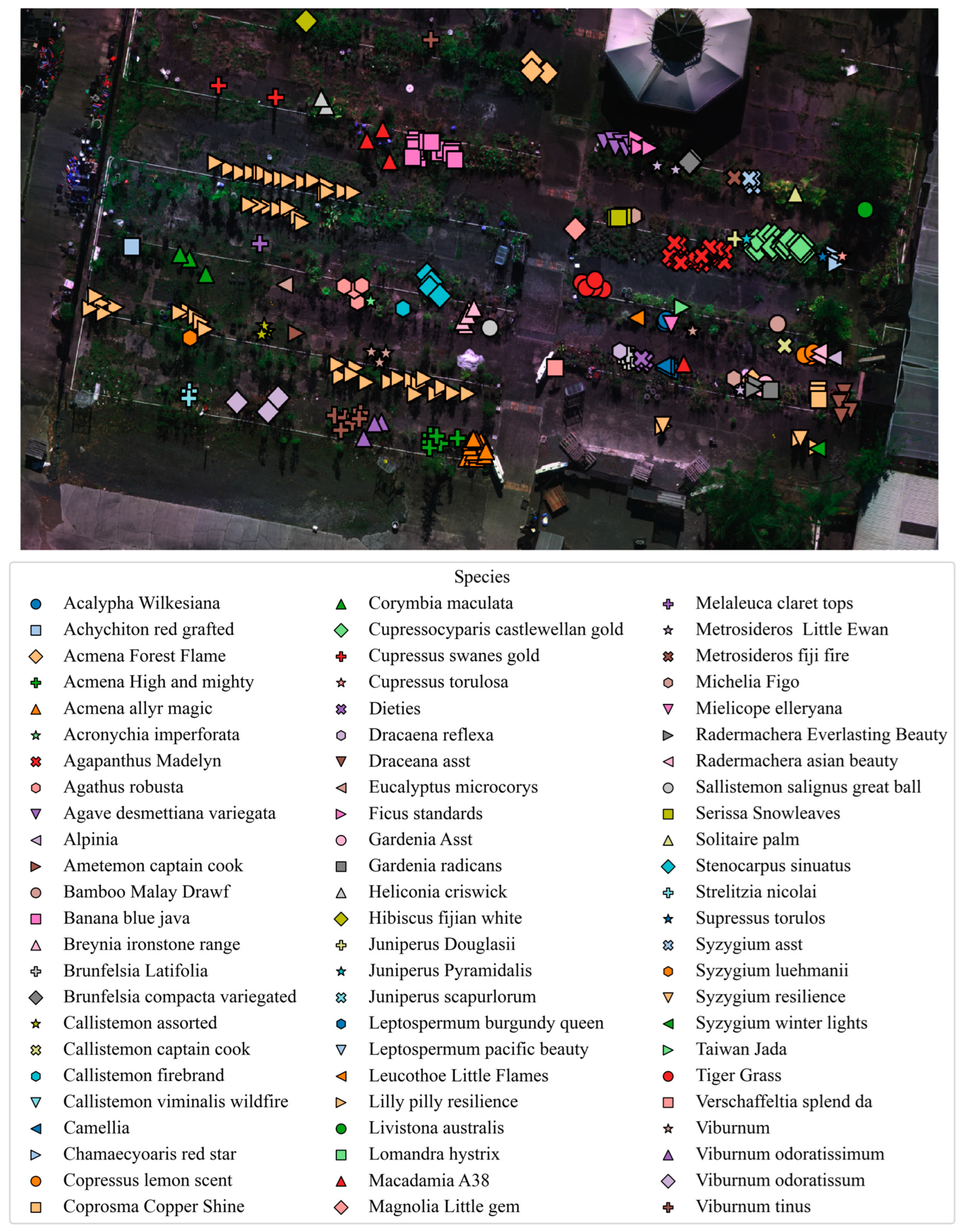
To ensure radiometric accuracy and consistent reflectance calibration, ground-based reference materials, including a 3 × 3 m white tarp and a reflective calibration pane, were used during data collection. Photogrammetric RGB imagery was captured using the DJI P1 sensor, achieving a ground sampling distance (GSD) of 3.5 mm from 23.89 m above ground level (AGL). MS data were acquired at 23.17 m AGL, resulting in a GSD of 10 mm. Additionally, the Hovermap ST-X LiDAR system was deployed at an altitude of approximately 35 m AGL. RTK-based ground control points (GCPs) were collected using an Emlid Reach RS2+ system to ensure high positional accuracy for georeferencing the UAS-derived datasets. A total of 72 individual vegetations were surveyed and spatially located within the study area, representing multiple ornamental species. Their distribution and identification are illustrated in Figure 3.
Figure 2. The study site: (a) Aerial map showing the site location, (b) Close-up bird’s-eye view from Nearmap, and (c) Side view captured at ground level using a DJI Mini 4. The red dashed line marks the region of interest.
Remotesensing 17 03454 g002

2.4. Individual Vegetation Delineation in 3D Point Clouds and Instance ID Map Generation
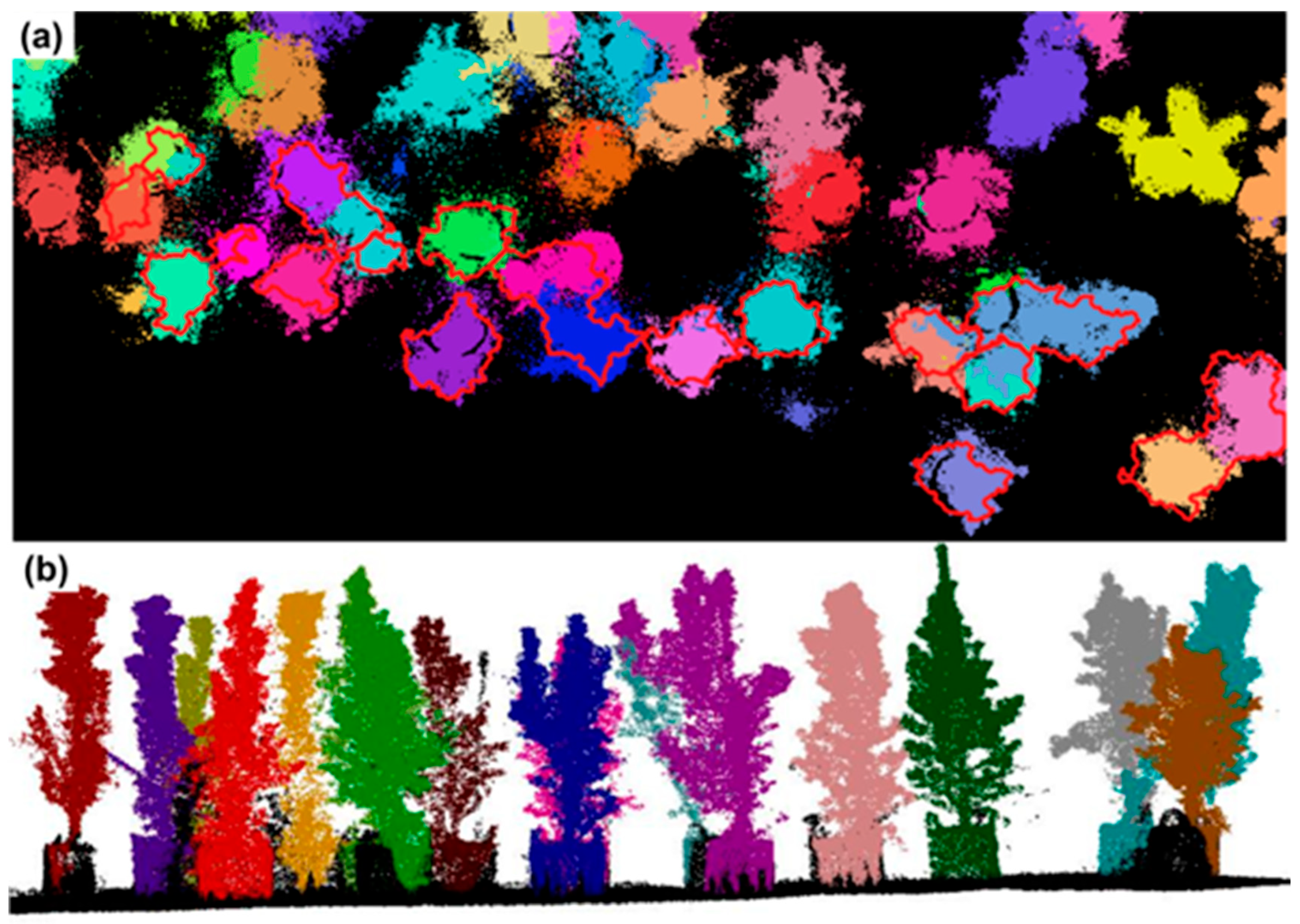
The fusion of aerial (UAS) and mobile terrestrial (hand-held) LiDAR has proven to be an effective method for detailed vegetation mapping [24]. However, its application becomes increasingly complex in environments with high species diversity and overlapping canopies, where distinguishing individual vegetations poses significant challenges [32]. To address this, point cloud segmentation was conducted using command-line tools within the Raycloudtools suite [40] (available at https://github.com/csiro-robotics/raycloudtools (accessed on 10 June 2025)), and its performance was benchmarked against manually segmented point clouds [24]. Raycloudtools generate the delineation of vegetation point clouds and provides individual vegetation attributes such as vegetation height (H) and crown diameter (D).
The process began with the generation of a ray cloud by integrating the raw LiDAR point cloud data with the UAS trajectory information. Ray cloud was then processed through the rayextract:trees tool from Raycloudtools, with a minimum H of 0.5 m to eliminate the low-lying grass and other vegetations. Each segmented vegetation using Raycloudtools was assigned a unique color to visually distinguish individual instances within the 3D point cloud. These colored segments were then projected onto a 2D plane to generate an Instance ID map, where each pixel represents a specific vegetation instance. This process ensures that all pixels corresponding to the same vegetation are uniquely grouped. Then segmented 3D data effectively transformed into a 2D raster format, enabling integration with other spatial data layers.
Figure 3. The location and the names of the outdoor vegetation species collected in the study site.
Remotesensing 17 03454 g003

2.5. Lilly Pilly Semantic Segmentation

2.5.1. Pixel Wise Labeling

Pixel-wise labeling was performed on 72 outdoor vegetation species; the Lilly Pilly species alone comprised 49 samples, using a combination of manual annotation and Normalized Difference Vegetation Index (NDVI) based thresholding. Areas with NDVI values below 0.35 were classified as non-vegetation. Due to the difficulty of visually distinguishing individual vegetation species in MS imagery alone, high-resolution RGB imagery (3.5 mm GSD) was also examined by annotators. The RGB imagery provided finer detail to accurately delineate vegetation boundaries. Vegetated and non-vegetated areas were marked using georeferenced vector polygons over the MS orthomosaic within a Geographic Information System (GIS) environment (QGIS 3.28 Firenze). Spectral band values for each class were extracted from the raster pixels of the georeferenced MS orthomosaic within the delineated polygons [31].

2.5.2. Ensemble Learning (EL)

EL is a robust ML paradigm that integrates multiple base models to improve predictive performance, enhance generalizability, and mitigate overfitting compared to individual learners [41]. In this study, an EL framework was implemented using four diverse base classifiers: Random Forest (RF), Support Vector Machine (SVM), eXtreme Gradient Boosting (XGBoost), and Light Gradient Boosting Machine (LightGBM). The XGBoost is used as the Meta model. These models were selected due to their proven strengths in handling high-dimensional data, non-linear relationships, and multiclass classification problems [42,43,44,45].
To construct the stacking ensemble architecture, the labeled MS data was divided into three subsets with a 60:20:20 split, corresponding to base training, base validation, and meta validation sets, respectively. Each base model was independently trained on the base training subset and evaluated on the base validation set. The meta-learner was trained using the combined 80% of the data (base training + base validation), where predictions from the base learners served as the input features. This two-level stacking strategy leverages the complementary strengths of the base models, enabling the meta-learner to correct individual model biases and improve classification robustness [46].
During class definition for classification, a noticeable variation in labeled pixel counts was observed across different vegetation types. This imbalance in the training data influenced model performance. To address this, vegetation classes for the segmentation model were selected based on their pixel count relative to Lilly Pilly. Specifically, vegetation types with pixel counts within ±50% of the Lilly Pilly pixel count were considered as individual classes. For species exceeding this threshold, their pixel data were randomly down sampled to match the Lilly Pilly pixel count. Remaining species that fell within the threshold range were grouped into a single “Other Vegetation” class, which was also balanced to the Lilly Pilly pixel count.
A suite of vegetation indices were derived to enhance class separability [24], namely, NDVI, Normalized Difference Water Index (NDWI), Normalized Difference Red Edge Index (NDRE), Green Chlorophyll Index (GCI), and Green Leaf Index (GLI) (Table 2). To further enrich the training data and enhance the model’s spatial robustness, a 3 × 3 pixel-level augmentation was applied [31]. This augmentation strategy expanded the training dataset by extracting nine overlapping patches centered around each labeled pixel, thus enabling the models to better capture local spectral-spatial variations within the MS imagery and reduce sensitivity to noise [47].

2.5.3. Generation of Lilly Pilly Patches

Although the ensemble classification model provided robust results, misclassifications were still noticeable around the canopy boundaries of Lilly Pilly, mainly due to overlapping vegetation structures and the spectral similarity of neighboring species. To address this, a watershed segmentation algorithm was implemented to enhance the spatial coherence of the classified masks. The watershed approach treats the pixel intensity values as a topographical surface and segments regions by simulating the process of water gradually flooding from local minima [48]. This method is particularly effective in separating connected or adjacent objects with subtle boundaries, such as intertwined vegetation canopies [49]. A dynamic threshold adjustment was performed, tuned based on visual inspection to generate the patches [50].

2.6. Development of Thermal Response Prediction Model

2.6.1. Determination of Thermal Properties of Lilly Pilly

Thermal properties were measured on milligram scale specimens using a simultaneous thermal analyzer that records thermogravimetric analysis (TGA) and differential scanning calorimetry (DSC) signals under controlled heating and atmospheres [51]. Arrhenius kinetic constants pre-exponential factor (A) and activation energy (E) were obtained from thermogravimetric (TG) mass loss curves collected under nitrogen using is conversional procedures. The same TGA runs provided the residual char mass fraction (Xchar) and the volatile yield by mass balance. The heat of pyrolysis was determined by integrating the DSC heat flow during oxygen free heating of the raw biomass with appropriate baseline corrections. Char produced in the inert run was preheated in oxygen and the exothermic integral gave the heat of char oxidation. The gross heat of combustion of the biomass was measured by bomb calorimetry. The specific heat of combustion of the volatile pyrolysates was then calculated by difference using the measured Xchar, the heat of char oxidation and the gross caloric value following established TG DSC based procedures in biomass thermochemistry.

2.6.2. Data Generation and Simulation

To generate the synthetic dataset, the Lilly Pilly was modeled with a conical crown shape, assuming a uniform distribution of foliage within the canopy. This approach was inspired by the study presented in [7]. Material and reaction data were mapped to FDS, (version 6.10.1) using the MATL (material), REAC (reaction), and SURF (surface) name lists. In MATL we specified the Arrhenius kinetic constants A and E for each solid-phase reaction together with the condensed-phase HEAT_OF_REACTION, the true solid DENSITY, and SPECIFIC_HEAT. Solid-phase product yields were assigned using SPEC_ID and NU_SPEC to generate the gaseous pyrolysates. The gas-phase combustion of the surrogate pyrolysate was then defined in REAC with the appropriate SPEC_ID_NU and HEAT_OF_COMBUSTION. For vegetative fuels, the MATL properties were paired on SURF with geometric and moisture descriptors, including SURFACE_VOLUME_RATIO and MOISTURE_FRACTION, and with aerodynamic resistance represented by DRAG_COEFFICIENT. The values for SURFACE_VOLUME_RATIO, SPECIFIC_HEAT, and DRAG_COEFFICIENT followed the examples and defaults in the current FDS User’s Guide and were adopted without modification [52]. All nomenclature and keyword usage follow the FDS User’s Guide [52,53]. A fixed vegetation moisture content of 14% was employed for the fire simulations to represent typical dry-season conditions that are correlated with elevated ignition potential during bushfire events. This selection is consistent with the findings of Nolan et al. [54] and subsequent analyses, which indicate that a dead fuel moisture threshold of approximately 14.6% delineates a critical ignition limit in New South Wales, Australia, below which vegetation exhibits a heightened susceptibility to combustion.
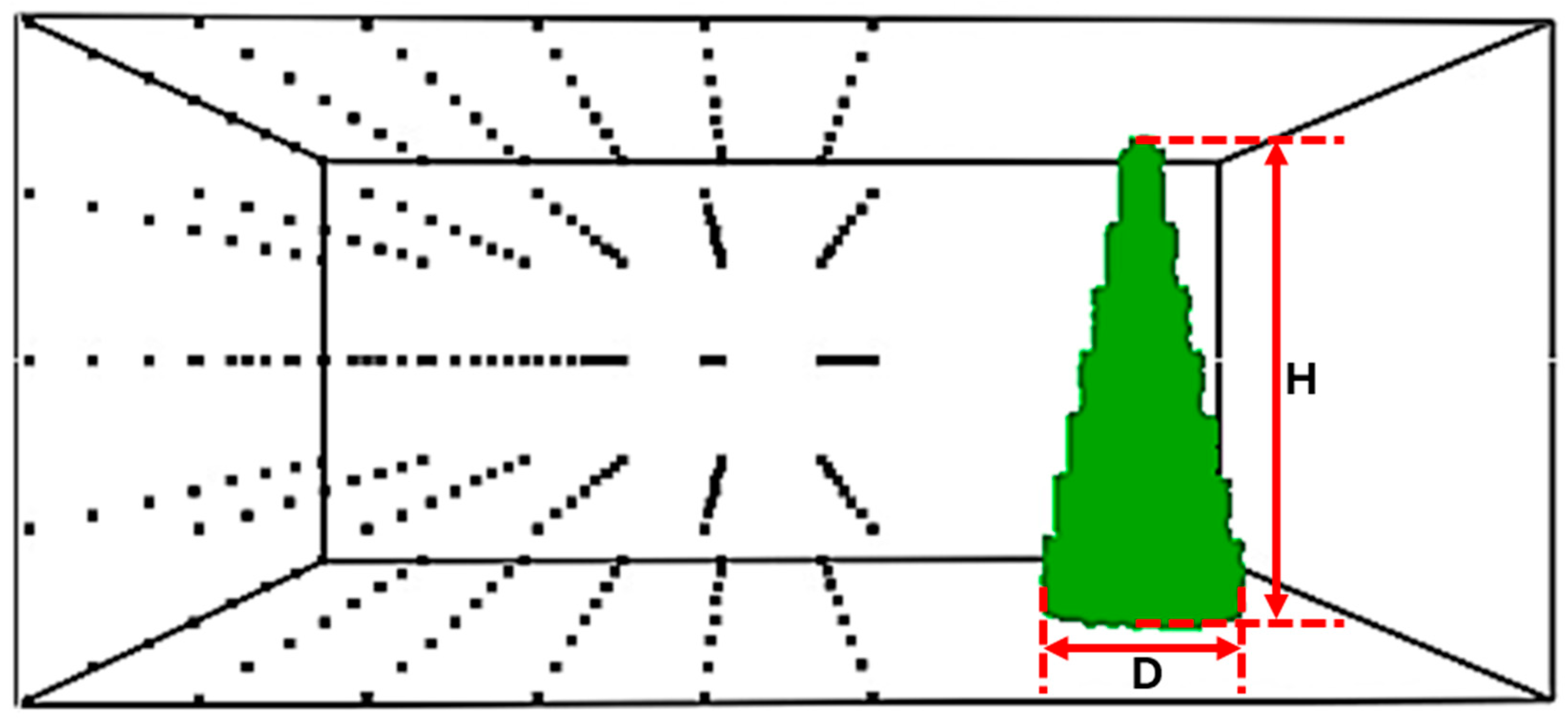
Vegetation dimensions, including H and D, were derived from the Raycloudtools based individual tree attributes in a region containing Lilly Pilly, as illustrated in Figure 4. Table 3 presents the derived dimensions of the selected 16 vegetation. These measurements informed the dimension range used for synthetic data generation in the simulation. The observed values ranged from 0.89 m to 1.36 m for H and from 0.298 m to 0.618 m for D. To ensure broader coverage and model generalizability, extended simulation ranges were defined as 0.5 m to 1.8 m for H and 0.2 m to 0.85 m for D. This resulted in a dataset comprising 13 D values and 27 H levels, yielding a total size of 351 vegetation 3D models. These extended ranges were used to generate voxelised models of synthetic vegetation for FDS simulation.
Each synthetic vegetation model was voxelised using a resolution of 0.05 m, aligning with the cell resolution used in FDS input formatting [53]. The spatial structure of the voxelised model was used to guide the placement of Lagrangian particles within the FDS model. The fuel elements are burnable particles inserted into each grid cell according to their coordinates in the simulation environment, along with their experimental thermal properties. This approach is consistent with the methodology adopted in the Douglas Fir tree modeling study conducted in [7]. The center of each vegetation was set to (1.8, 0.8, 0.0) in the simulation space which ranges for (0, 3.6), (0, 4.5), (0, 2) along the XYZ planes. The simulations were performed with a 3D sensor-based grids, mimicking realistic detection of HF, and T distribution at the surrounding [55]. The sensor grid bounds (0, 3.5), (2, 4.5), (0, 2) margins with a resolution of 0.5 m, through XYZ planes, respectively. The HF sensors were oriented in the direction of Y (0, −1, 0), facing toward the burning particles. Figure 5 illustrates the vegetation alongside the sensor grid layout.
Each simulation was run for a total duration of 60 s, with the ignition set for a 5 s period using a ring-shaped burner ignition setup. We set the flame-zone temperature to 1500 K, which is consistent with reported cellulosic flame temperatures (~1200–1600 K) and in-flame bushfire measurements (~800–1200 °C) [56]. For the pilot, we used a ring burner to achieve uniform base ignition and specified HRRPUA = 60 kW·m−2 for 5 s. NIST’s Douglas-fir tree tests [7] employed burner exposures of 30 kW·m−2 for 10 s and 60 kW·m−2 for 30 s; in our case, we selected the upper flux (60 kW·m−2) but a shorter duration (5 s) to minimize potential bias in T/HF measurements while still providing a strong, reliable pilot. FDS simulations conducted in this study were executed on the QUT virtual machine infrastructure. Specifically, simulations ran on a high-performance system identified as ERES-GEN11-122, equipped with an AMD EPYC 9474F 48-Core Processor operating at 3.60 GHz and supported by 64.0 GB of installed RAM.

2.6.3. Thermal Response Prediction Model Training

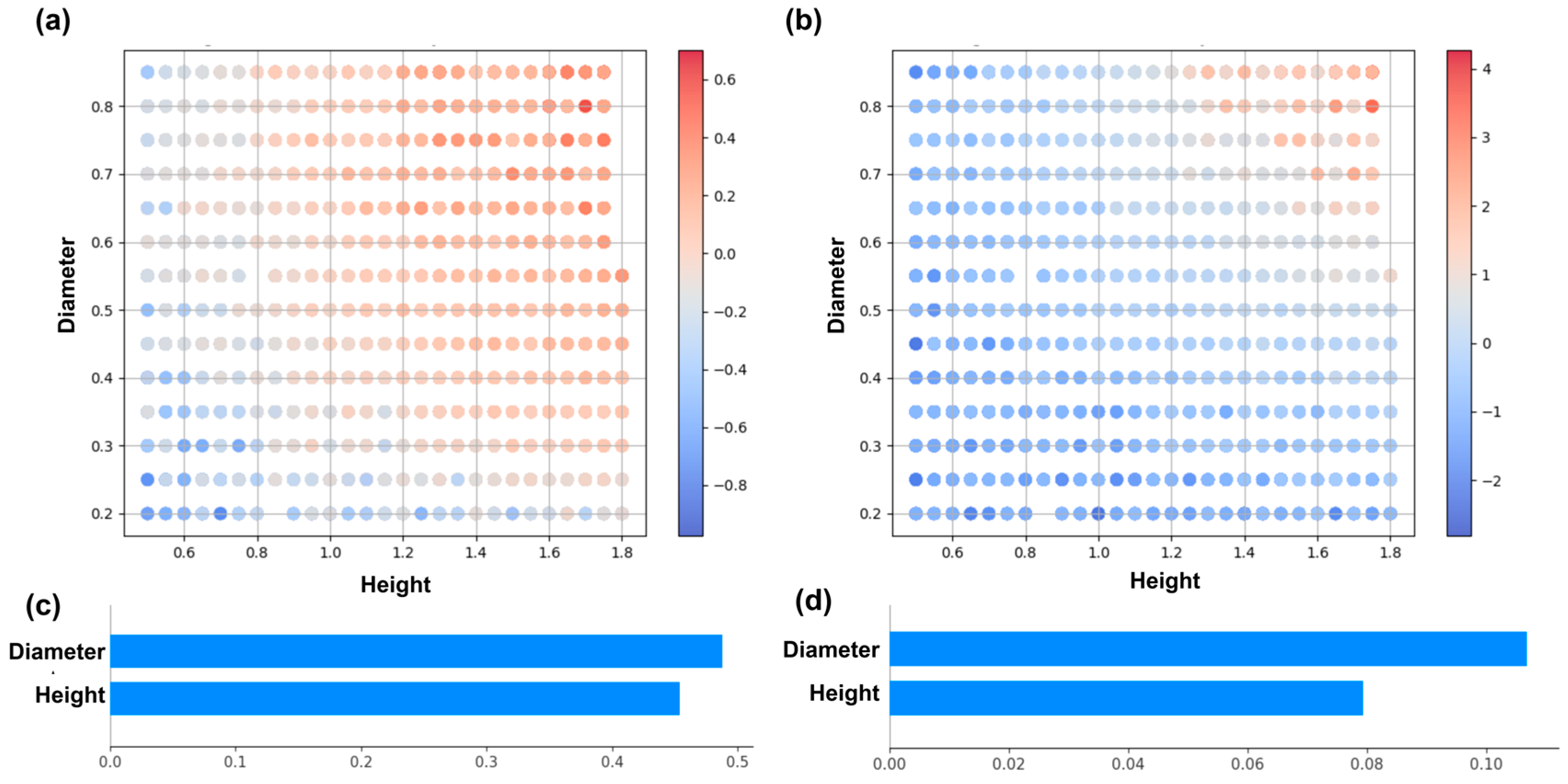
Following the generation of synthetic vegetation data and completion of the FDS runs the thermal response (output) maximum values (T and HF) were extracted for ML model training. The objective was to predict thermal behavior (T and HF) based on a given vegetation’s geometric characteristics (D and H). To evaluate the predictive performance of thermal responses, the dataset was split into a training and testing set using an 80:20 ratio [57]. The XGBoost [44] model was trained using FDS-generated sensor data to learn non-linear relationships between fire characteristics and sensor outputs, enabling fast and accurate predictions without rerunning computationally intensive simulations. The model was trained using input features including H, D, and the sensor’s Cartesian coordinates (X, Y, Z) representing its distance from the vegetation base, while the target variables were T and HF (Maximum values recorded in the sensors), as obtained from the FDS simulation outputs. To optimize model performance, hyperparameter tuning was performed during the training process. To further assess potential systematic bias in model predictions, SHAP (SHapley Additive exPlanations), an explainable AI framework analysis was conducted to evaluate the influence of vegetation H and D on predicted T and HF [58]. SHAP offers both local explanations, which detail feature impact for individual predictions, and global interpretations, which assess average feature importance across the dataset.

2.6.4. Thermal Response Prediction and Application

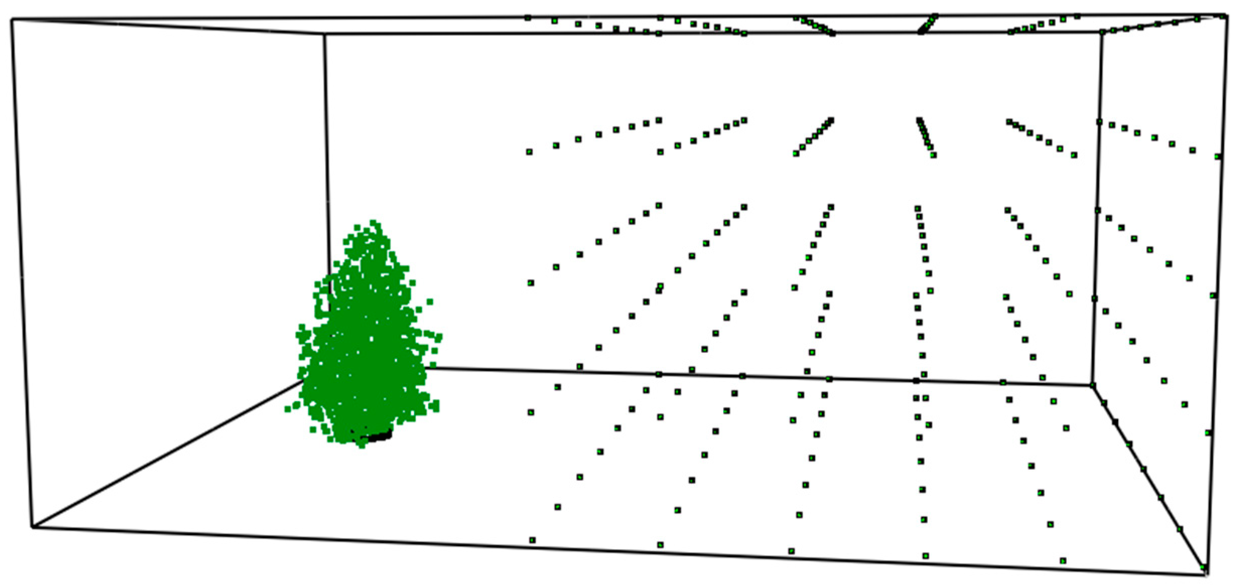
Lilly Pilly vegetation samples from the study site were selected to compare the results of the simulation with model-based predictions. The point cloud of this vegetation was voxelised at a resolution of 0.05 m and simulated using the same setup described in Section 2.6.2. The voxelised Lilly Pilly point cloud of a vegetation, with tree ID 4, within the FDS simulation environment is shown in Figure 6. The vegetation attributes, including H and D, were measured and used as inputs to the developed thermal response prediction model.

3. Results

3.1. Lilly Pilly Semantic Segmentation Performance

A total of 11 classes were utilized for model development, comprising 9 distinct vegetation classes, an “Other Vegetation” class that aggregated all vegetation types with pixel counts below 50% of that of Lilly Pilly, and a “non-vegetation” class. Table 4 summarizes the selected hyperparameter settings for both the base and the meta model within the proposed EL framework. The performance of semantic segmentation employing EL was evaluated by assessing each base model on the validation datasets, while the meta-model was subsequently tested on the test dataset. Table 5 details the classification performance metrics of each base model and the meta-model for the Lilly Pilly segmentation, reporting accuracy, precision, recall, and F1-score. Among the base models, CatBoost and XGBoost achieved higher F1-scores, indicating stronger performance in terms of both precision and recall.
Table 6 presents the number of pixels and the vegetation species utilized in the EL model. Lilly Pilly had one of the highest pixel counts (64,359) and achieved an F1 score of 0.7634, showing moderate classification performance compared to others like Callistemon viminalis wildfire (F1 = 0.9722) and Solitaire palm (F1 = 0.9463). Although Lilly Pilly was well-represented in the dataset, some less-represented species with lower support showed higher precision and recall, indicating stronger separability in the feature space.
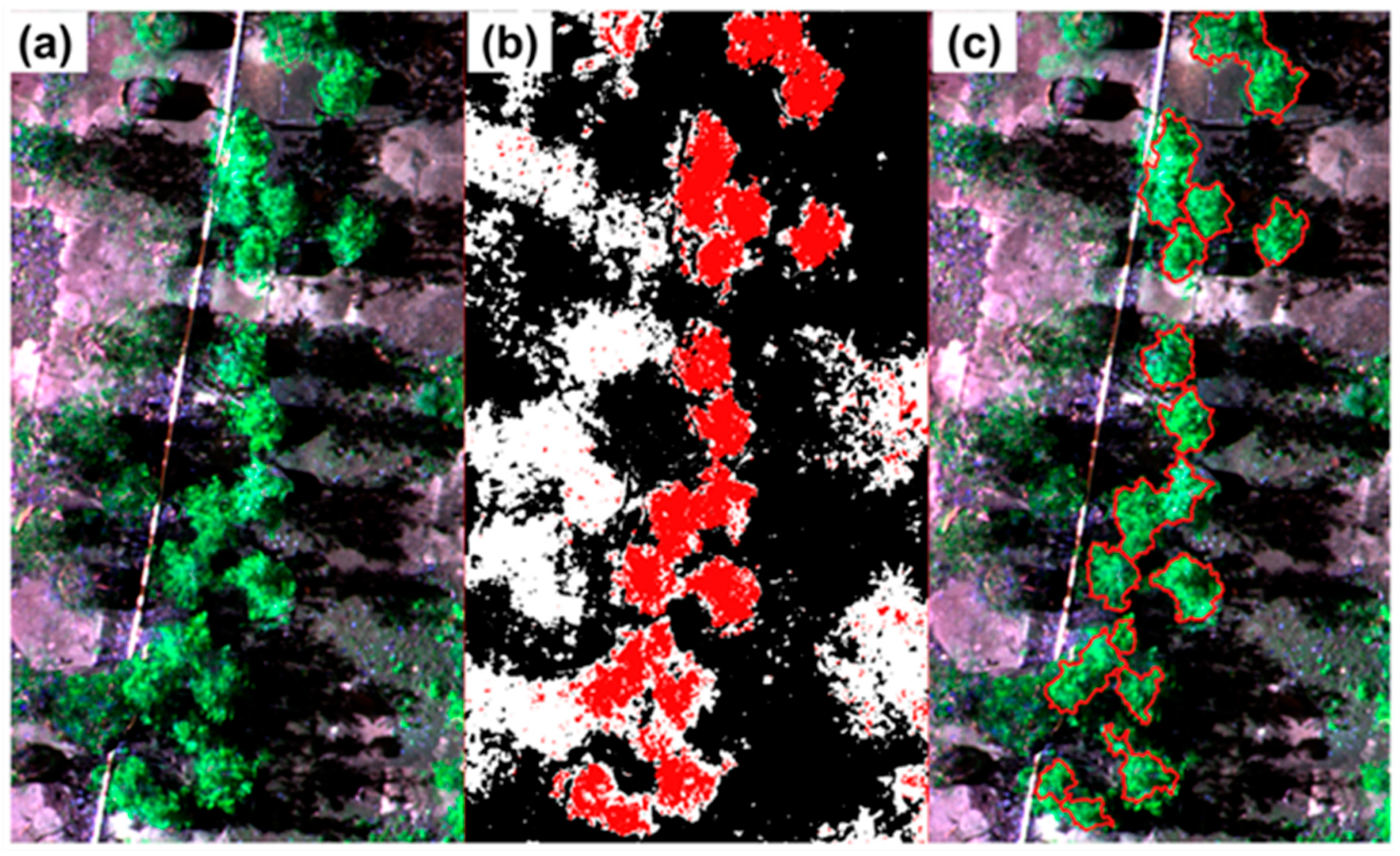
The segmentation outcomes are visualized in, displaying the semantic segmentation map produced by the meta-model. While some misclassifications are presented in Figure 7b, they are primarily concentrated in the region containing Lilly Pilly vegetation. Figure 7c demonstrates its efficacy in successfully delineating all Lilly Pilly regions as distinct patches within the MS imagery.

3.2. Instance-Based Vegetation Segmentation and Filtering Lilly Pilly

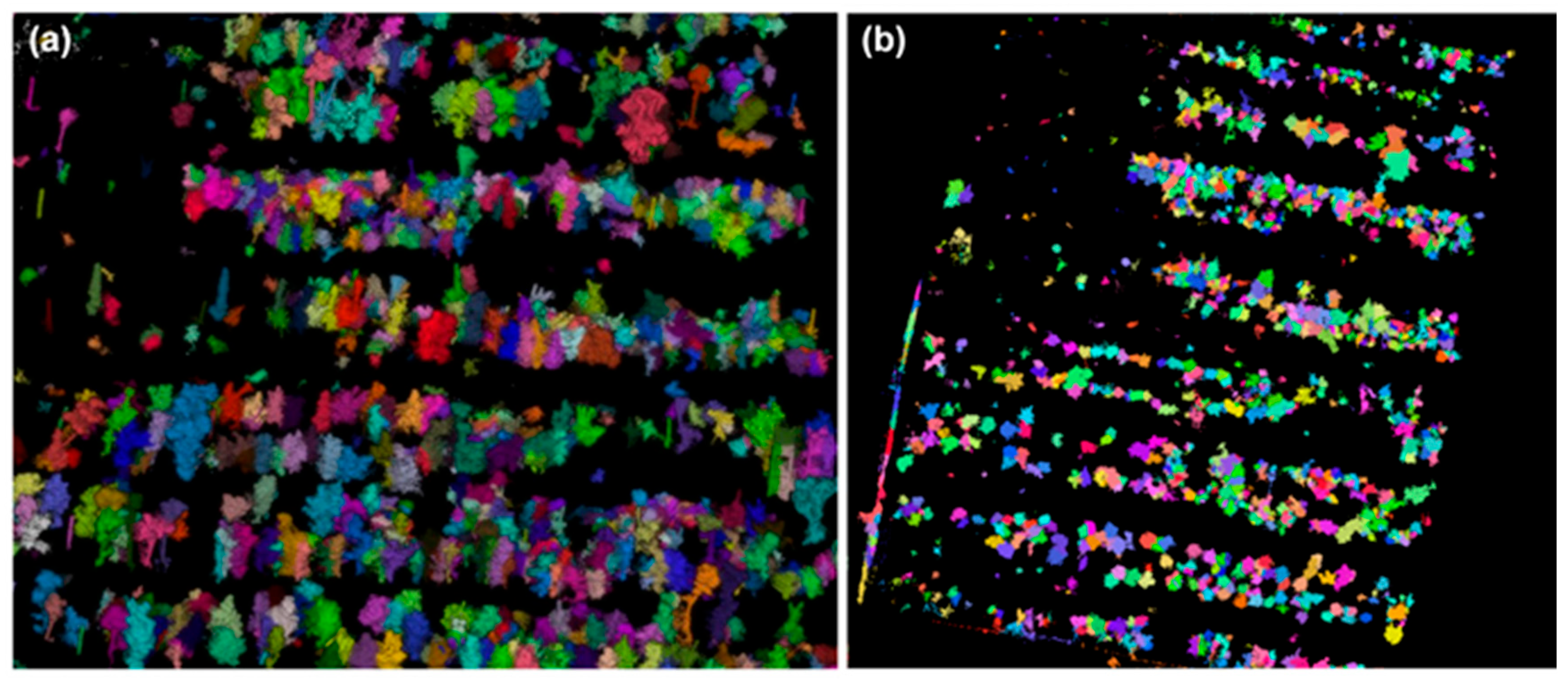
Figure 8a displays the segmented LiDAR point cloud output from Raycloudtools, while Figure 8b presents the corresponding 2D projected instance ID map, where each vegetation region is color-coded and assigned a unique identifier. The patches derived from the watershed algorithm effectively filtered all Lilly Pilly vegetation falling within the same geospatial boundaries. Figure 9a shows the alignment of Lilly Pilly patches identified by the semantic segmentation model (EL), and Figure 9b illustrates the filtered vegetation point cloud instances, capturing all Lilly Pilly vegetations within the defined test region.

3.3. Thermal Response Prediction

The simulation of each FDS file, corresponding to 351 vegetation files of varying dimensions, took between 16 and 17 min to complete. Figure 10 shows the 3D sensor grid, sliced planes, and the recorded maximum thermal responses (T and HF) from the sensors for a synthetic vegetation model with an H of 1.15 m and a D of 0.8 m. Thermal response prediction model exhibited high predictive accuracy on both the training and validation sets. For T prediction on the training data, achieved a root mean square error (RMSE) of 0.0547 and a coefficient of determination (R2) of 0.9971. Similarly, for HF prediction, recorded an RMSE of 0.1372 and an R2 of 0.9933. Figure 11 shows the SHAP analysis results, illustrating how vegetation height and diameter influence the model’s predictions of T and HF.

3.4. Comparison of Predicted Thermal Response
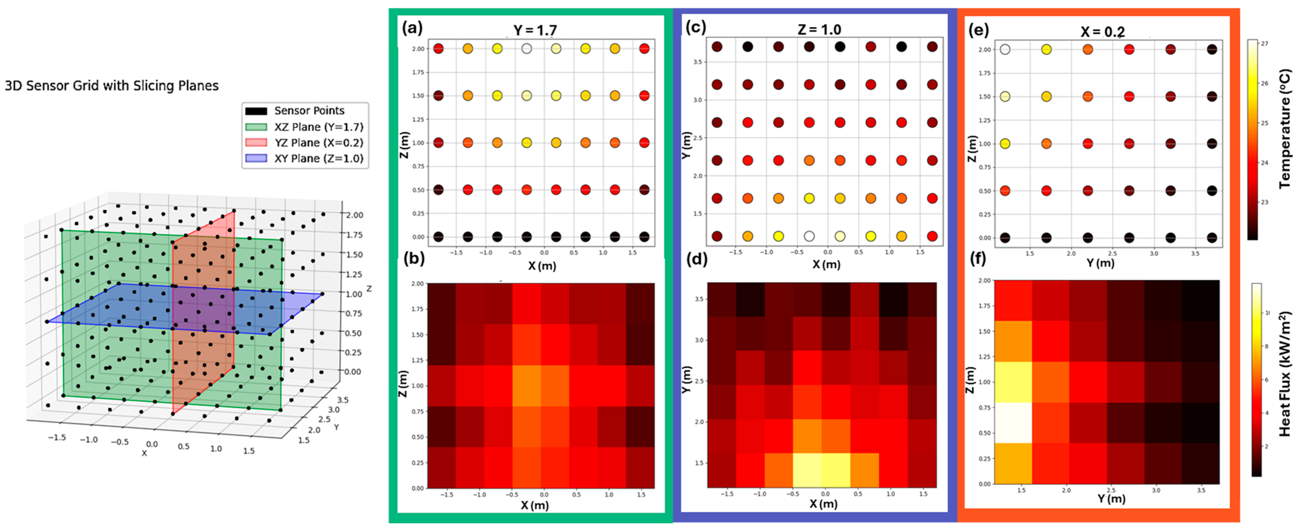
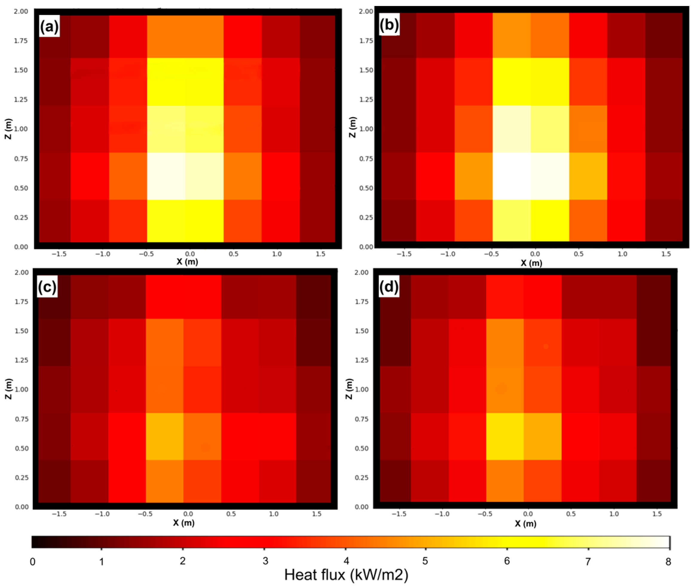
Figure 12 and Figure 13 illustrate the comparison between actual and model-predicted thermal responses, HF and T across two critical cross-sections of a Lilly Pilly vegetation canopy (Y = 1.2 m and Y = 1.7 m). At Y = 1.2 m. The model demonstrated strong validation performance using the simulated vegetation geometry derived from the point cloud, achieving an RMSE of 0.2435 and R2 of 0.9200 for T, and an RMSE of 0.3384 and R2 of 0.9463 for HF, for the selected vegetation with a height of 0.97 m and a diameter of 0.604 m. The RMSE values for the target variable T and HF across other vegetation samples are provided in Table 7.
Figure 10. Sensor grid planes for a sample Lilly Pilly with H and D values of 1.15 m and 0.85 m, respectively: (a) T heatmap across XZ plane at Y = 1.7 m; (b) HF heatmap across XZ plane at Y = 1.7 m; (c) T heatmap across XY plane at Z = 1 m; (d) HF heatmap across XY plane at Z = 1 m; (e) T heatmap across YZ plane at X = 0.2 m; (f) HF heatmap across YZ plane at X = 0.2 m.
Remotesensing 17 03454 g010
Figure 11. SHAP analysis of model predictions for T and HF: (a) Height vs. diameter colored by SHAP values for T prediction, (b) Height vs. diameter colored by SHAP values for HF prediction, (c) SHAP feature importance map for height and diameter showing the mean (|SHAP value|) as the average impact on model T prediction, and (d) SHAP feature importance map for height and diameter showing the mean (|SHAP value|) as the average impact on model HF prediction.
Remotesensing 17 03454 g011
Table 7. Validation results showing RMSE values between the FDS-simulated and predicted temperature (T) and heat flux (HF) across vegetation samples in the test region.
Tree IDRMSE
THF
10.49160.4996
20.18940.3055
30.54521.2341
40.24350.3384
50.18940.3055
60.22020.3206
70.5670.9070
80.5330.4624
90.19040.3389
100.5330.4624
110.43580.7644
120.18110.390
130.24820.5056
140.49590.7410
150.18940.3055
160.17840.5190
Figure 12. Visualization of actual and predicted HF distributions across the XZ plane at two Y-axis cross-sections (Y = 1.2 m and Y = 1.7 m) for a sample Lilly Pilly vegetation: (a) Actual HF distribution at Y = 1.2 m; (b) Predicted HF distribution at Y = 1.2 m; (c) Actual HF distribution at Y = 1.7 m; (d) Predicted HF distribution at Y = 1.7 m.
Remotesensing 17 03454 g012
Figure 13. Visualization of actual and predicted T distributions across the XZ plane at two Y-axis cross-sections (Y = 1.2 m and Y = 1.7 m) for a sample Lilly Pilly vegetation: (a) Actual T distribution at Y = 1.2 m; (b) Predicted T distribution at Y = 1.2 m; (c) Actual T distribution at Y = 1.7 m; (d) Predicted T distribution at Y = 1.7 m.
Remotesensing 17 03454 g013

4. Discussion

This study demonstrates the feasibility of the proposed framework using a single vegetation species and standardized ignition conditions in fire simulations. It highlights the potential of combining multisensory RS (UAS-based MS and LiDAR) with FDS and ML to assess the maximum values of thermal response prediction (T and HF) for an outdoor vegetation species, particularly the Lilly Pilly. The results obtained from semantic segmentation, individual tree delineation in 3D point clouds, and FDS-based thermal simulations highlight the effectiveness of integrating spatial data and ML for vegetation-specific fire modeling.
In the past decade, the fusion of LiDAR and photogrammetry data in RS has emerged as a promising approach for improving accuracy and enriching information for ML–based vegetation segmentation and forest attribute estimation [59]. fusion methodologies are predominantly classified into two categories: data-level fusion and feature-level fusion. Data-level fusion involves the integration of raw data from multiple sensors prior to any processing. This involves merging airborne and torrential LiDAR datasets [60] or co-registration of multisource data using GCP and similar features. The majority of existing studies utilize feature-level fusion [59], where features are extracted separately from each data source and then combined for joint modeling. In the studies by Sankey et al. [61], Norton et al. [62] and Hall & Lara [63] LiDAR data were converted into raster formats to create canopy height models (CHM) and digital terrain models (DTM). These raster layers were then combined with MS and HS bands to serve as input for ML classification algorithms. Some studies took a slightly different approach. Plakman et al. [64] and Zhang et al. [65] applied watershed segmentation on CHMs using satellite data to delineate individual tree crowns, while Qin et al. [66] used the same approach with UAV imagery. The resulting tree boundaries were subsequently used to extract spectral information for individual vegetation detection ML models. However, the final outputs of such models inherently face confidence limitations because they do not achieve 100% accuracy. This uncertainty emphasizes the importance of complementary methods to refine and validate point cloud delineation of specific species for accurate estimation of vegetation attributes such as H and D.
Our study presents a decision-level fusion approach [67]. Rather than directly combining raw data or extracted features, this method processes MS imagery and LiDAR data independently in separate workflows and then merges their results (decisions) to produce the final segmentation of Lilly Pilly. This method improves accuracy by combining EL segmentation with traditional image processing and advanced point cloud delineation tools. Although the ML model achieved a 79% F1 score in segmenting Lilly Pilly vegetation in MS imagery, it is not fully accurate alone. Applying a watershed algorithm to the segmentation results clearly defines the spatial boundaries of vegetation patches. These patches are then used to filter the vegetation point clouds delineated from the 3D point cloud using Raycloudtools. This approach ensures that only the point clouds corresponding to Lilly Pilly within the test region are selected, resulting in a more complete and precise segmentation. While [29,55] applied general fuel models for shrubs or trees, our work incorporated experimental solid-phase parameters (density, specific heat, Arrhenius kinetics) derived from STA, leading to higher fidelity in fire behavior prediction. This application of predictive modeling directly to remote sensing-derived structural features facilitates non-destructive thermal risk estimation of individual vegetations, enabling scalable and site-specific wildfire vulnerability assessment [68,69].
Mell et al. [7] demonstrated the capability of FDS to represent the spatial distribution of vegetation, validating it through controlled tree-burning experiments using Douglas fir with a conical crown and uniformly distributed fuel cells. Building upon this foundation, Moinuddin et al. [70] employed a particle-based fuel modeling approach for Douglas fir, further substantiating its applicability. In our previous study [24], we segmented distinct structural components of a 29 m tall Eucalyptus siderophloia, utilizing Lagrangian particle models to represent foliage. In the present study, we place particular emphasis on an outdoor vegetation, Lilly Pilly, wherein the entire structure is treated as foliage. We adapted a validated particle-based representation and laboratory-measured thermal properties of Lilly Pilly in our simulations to generate physically realistic training data for the thermal response prediction model. Utilizing this simulated dataset, the model achieved high predictive accuracy, with temperature predictions yielding an R2 of 0.9971, while heat flux predictions achieved an R2 of 0.9933 on the validation set. This strong predictive performance demonstrates that our approach can address one of the major limitations of physics-based simulations: the prohibitively large computational cost associated with the extremely fine grid resolution required [70], while enabling the efficient generation of extensive datasets.

5. Limitations and Future Work

Despite the promising results of this study, several limitations must be addressed to further enhance the robustness and applicability of the proposed thermal response prediction. The current study primarily provides a feasibility validation of the framework using idealized cone-shaped corn models. In practice, these vegetations are not always maintained in conical shapes. To move beyond this assumption and adapt the framework to other vegetation shapes, a synthetic dataset with rectangular or trapezoidal shapes spanning a range of dimensions would need to be generated. Simulation results from these datasets can then be used to train the model to predict thermal responses from geometric dimensions. For extracting the dimensions of fitted 3D, shape-fitting algorithms such as BEES [71] and RANSAC [72] can be applied after isolating individual vegetation point cloud from semantic segmentation-based plant patches.
The current methodology has been validated only by Lilly Pilly. For broader applicability and reproducibility of the model, it is essential to expand the scope to include multiple vegetation species, each classified into distinct fire behavior classes. However, generalization of the framework and adaptation to other vegetation species is limited by the lack of literature-based thermal property data required for accurate simulations. Experimental determination of species-specific thermal properties is critical to enable the application of the framework to other vegetation types.
Semantic segmentation was performed using high-resolution MS imagery captured at relatively low drone altitudes (20–30 m AGL). However, in practical field deployments, flying at such low altitudes may be restricted due to regulatory, safety, or terrain constraints. Therefore, the performance of segmentation and classification models should be tested on lower-resolution imagery captured from higher altitudes to evaluate the transferability and robustness of the method under realistic application conditions. The altitude of UAV flights influences the density of point clouds and spatial resolution of orthomosaic maps. Lower-resolution point clouds may diminish the accuracy of height and diameter estimations, which could adversely affect predictive outcomes. However, the incorporation of ground-based LiDAR acquisition can enhance point cloud density and improve accuracy. On the other hand, HS data provides significantly higher spectral resolution, though it sacrifices some spatial detail. Our previous study [31] assessed the effectiveness of MS and HS imagery for segmenting African lovegrass in a mixed environment. However future work should include a comparative analysis between MS, HS, and photogrammetric sensors to evaluate the trade-offs in spatial-spectral resolution and their impact on segmentation accuracy for outdoor species.
Currently, the ignition is set at the center and bottom of the vegetation with zero wind speed. However, ignition location, vegetation moisture, wind speed and direction, and reflection or shielding from nearby surfaces can all influence heat release. Application of this methodology should incorporate these factors to enhance the framework’s robustness under varying regional and seasonal trends in moisture content and weather conditions. Species-specific seasonal variations in vegetation moisture content can be quantified through systematic destructive sampling and correlated with spectral vegetation indices [73]. Collectively, addressing these limitations will strengthen the scalability and reliability of the proposed framework, paving the way for practical use in wildfire risk assessment across diverse environments and vegetation types.

6. Conclusions

This study aims to develop a UAS-based RS approach to address the challenges of understanding the thermal responses of burning vegetation near residential structures, with a focus on a common Australian native vegetation, Lilly Pilly. First, a hybrid segmentation pipeline integrating ML, watershed algorithm, and Raycloudtools were used to accurately delineate Lilly Pilly vegetation in 3D point clouds, effectively overcoming the performance limitations of standalone ML models. Second, the segmented vegetation data were used to characterize the dimensions of Lilly Pilly and generate synthetic datasets for FDS simulation, which supported the development of a predictive model for the maximum thermal responses, T and HF, at varying distance from the vegetation. The watershed algorithm applied to EL based semantic segmentation results on high-resolution MS imagery facilitated the generation of patches represented as geospatial vector polygons outlining the Lilly Pilly crowns. Using these location-based patches to filter the vegetation point clouds delineated by Raycloudtools effectively extracted the Lilly Pilly point clouds from the study sites. The results underscore the potential of integrating UAS-based RS, ML based segmentation, and fire dynamics modeling to assess building risk from nearby burning vegetation. The generalization of the framework is constrained by the following limitations.
  • The framework was validated based on the assumption that Lilly Pilly is pruned into a cone shape, whereas real Lilly Pilly vegetation can be maintained in varied geometries, such as rectangular or trapezoidal prisms.
  • The study was applied only to Lilly Pilly, and the lack of thermal property data limits adaptation to other species.
  • Vegetation semantic segmentation relies on high-resolution imagery and using different sensors or higher-altitude imagery may affect the segmentation performance.
To enhance generalizability and improve the framework’s potential applicability, future work should incorporate a broader range of vegetation species, adopt different shapes vegetations, utilizing imagery from higher flight altitudes, and exploring the use of HS data for improved spectral discrimination in outdoor vegetation segmentation. Overall, this research establishes a foundation for a scalable framework that can be refined for broader applications in estimating the fire risk posed by surrounding vegetation.

Author Contributions

Conceptualization, P.K.; methodology, P.K. and I.K.S.; software, P.K., I.K.S. and T.K.; validation, P.K.; formal analysis, P.K., I.K.S. and T.K.; investigation, P.K.; resources, P.K., A.A., G.H. and F.G.; data curation, P.K. and I.K.S.; writing—original draft preparation, P.K., I.K.S. and T.K.; writing—review and editing, P.K., I.K.S., T.K., A.A., G.H. and F.G.; visualization, P.K. and I.K.S.; supervision, A.A., G.H. and F.G.; project administration, A.A., G.H. and F.G.; funding acquisition, A.A., G.H. and F.G. All authors have read and agreed to the published version of the manuscript.

Funding

This project is supported through funding from ARC Discovery program (Project number: DP 220103233).

Data Availability Statement

Data relevant to this study, including the UAS-collected data and laboratory tests on the thermal properties of Lilly Pilly can be provided upon request.

Acknowledgments

We wish to thank the Australian Research Council (ARC) and Queensland University of Technology (QUT) for providing financial support and laboratory facilities. The authors gratefully acknowledge the support of Nurso staff for data collection and species identification. We also wish to acknowledge the support of the Research Engineering Facility (REF) team at QUT for the provision of expertise and research infrastructure and gratefully acknowledge QUT’s High-Performance Computing (HPC) facility for enabling this project. We thank Hexagon for providing access to the SmartNet RTK corrections service to support the precise survey of GCPs.

Conflicts of Interest

The authors declare no conflicts of interest.

References

  1. Moritz, M.; Batllori, E.; Bradstock, R.A.; Gill, A.M.; Handmer, J.; Hessburg, P.F.; Leonard, J.; McCaffrey, S.; Odion, D.C.; Schoennagel, T.; et al. Learning to coexist with wildfire. Nature 2014, 515, 58–66. [Google Scholar] [CrossRef] [PubMed]
  2. Westerling, A. Increasing western US forest wildfire activity: Sensitivity to changes in the timing of spring. Philos. Trans. R. Soc. B Biol. Sci. 2016, 371, 20150178. [Google Scholar] [CrossRef]
  3. Ottmar, R.D. Wildland fire emissions, carbon, and climate: Modeling fuel consumption. For. Ecol. Manag. 2014, 317, 41–50. [Google Scholar] [CrossRef]
  4. Bradstock, R.A. A biogeographic model of fire regimes in Australia: Current and future implications. Glob. Ecol. Biogeogr. 2010, 19, 145–158. [Google Scholar] [CrossRef]
  5. Baker, W.L.; Mladenoff, D.J. Progress and future directions in spatial modeling of forest landscapes. In Spatial Modeling of Forest Landscape Change; Cambridge University Press: Cambridge, UK, 1999; pp. 333–349. [Google Scholar]
  6. Cohen, J.D. Preventing disaster: Home ignitability in the wildland-urban interface. J. For. 2000, 98, 15–21. [Google Scholar] [CrossRef]
  7. Mell, W.; Maranghides, A.; McDermott, R.; Manzello, S.L. Numerical simulation and experiments of burning douglas fir trees. Combust. Flame 2009, 156, 2023–2041. [Google Scholar] [CrossRef]
  8. Benedict, K.B.; Lee, J.E.; Kumar, N.; Badal, P.S.; Barbato, M.; Dubey, M.K.; Aiken, A.C. Wildland Urban Interface (WUI) Emissions: Laboratory Measurement of Aerosol and Trace Gas from Combustion of Manufactured Building Materials. ACS ES&T Air 2024, 1, 1673–1686. [Google Scholar] [CrossRef]
  9. Zhou, A. Performance evaluation of ignition-resistant materials for structure fire protection in the WUI. In Proceedings of the 13th International Conference and Exhibition on Fire and Materials (Fire and Materials 2013), San Francisco, CA, USA, 28–30 January 2013; pp. 355–366. [Google Scholar]
  10. Caton, S.E.; Hakes, R.S.P.; Gorham, D.J.; Zhou, A.; Gollner, M.J. Review of Pathways for Building Fire Spread in the Wildland Urban Interface Part I: Exposure Conditions. Fire Technol. 2017, 53, 429–473. [Google Scholar] [CrossRef]
  11. Intini, P.; Ronchi, E.; Gwynne, S.; Bénichou, N. Guidance on Design and Construction of the Built Environment Against Wildland Urban Interface Fire Hazard: A Review. Fire Technol. 2020, 56, 1853–1883. [Google Scholar] [CrossRef]
  12. Finney, M.A. FARSITE, Fire Area Simulator—Model Development and Evaluation; U.S. Department of Agriculture, Forest Service, Rocky Mountain Research Station: Ogden, UT, USA, 1998. [Google Scholar]
  13. Salis, M. Fire Behaviour Simulation in Mediterranean Maquis Using FARSITE (Fire Area Simulator). Ph.D. Thesis, University of Sassari, Sardinia, Italy, 2008. [Google Scholar]
  14. Andrews, P.L.; Bevins, C.D.; Seli, R.C. BehavePlus Fire Modeling System, Version 4.0: User’s Guide; General Technical Report, RMRS-GTR-106 Revised; Department of Agriculture, Forest Service, Rocky Mountain Research Station: Ogden, UT, USA, 2005; Volume 106, 132p. [Google Scholar]
  15. Tolhurst, K.; Shields, B.; Chong, D. Phoenix: Development and application of a bushfire risk management tool. Aust. J. Emerg. Manag. 2008, 23, 47–54. [Google Scholar]
  16. Salamí, E.; Barrado, C.; Pastor, E. UAV Flight Experiments Applied to the Remote Sensing of Vegetated Areas. Remote Sens. 2014, 6, 11051–11081. [Google Scholar] [CrossRef]
  17. Huot, F.; Hu, R.L.; Goyal, N.; Sankar, T.; Ihme, M.; Chen, Y.F. Next Day Wildfire Spread: A Machine Learning Dataset to Predict Wildfire Spreading From Remote-Sensing Data. IEEE Trans. Geosci. Remote Sens. 2022, 60, 4412513. [Google Scholar] [CrossRef]
  18. Camps-Valls, G.; Tuia, D.; Bruzzone, L.; Benediktsson, J.A. Advances in Hyperspectral Image Classification: Earth Monitoring with Statistical Learning Methods. IEEE Signal Process. Mag. 2014, 31, 45–54. [Google Scholar] [CrossRef]
  19. Kanand, T.; Kemper, G.; König, R.; Kemper, H. Wildfire Detection and Disaster Monitoring System Using UAS and Sensor Fusion Technologies. Int. Arch. Photogramm. Remote Sens. Spat. Inf. Sci. 2020, 43, 1671–1675. [Google Scholar] [CrossRef]
  20. Ganteaume, A.; Guillaume, B.; Girardin, B.; Guerra, F. CFD modelling of WUI fire behaviour in historical fire cases according to different fuel management scenarios. Int. J. Wildland Fire 2023, 32, 363–379. [Google Scholar] [CrossRef]
  21. Mell, W.; Jenkins, M.A.; Gould, J.; Cheney, P. A physics-based approach to modelling grassland fires. Int. J. Wildland Fire 2007, 16, 1–22. [Google Scholar] [CrossRef]
  22. Anderson, W.R.; Cruz, M.G.; Fernandes, P.M.; McCaw, L.; Vega, J.A.; Bradstock, R.A.; Fogarty, L.; Gould, J.; McCarthy, G.; Marsden-Smedley, J.B.; et al. A generic, empirical-based model for predicting rate of fire spread in shrublands. Int. J. Wildland Fire 2015, 24, 443–460. [Google Scholar] [CrossRef]
  23. Fiorini, C.; Craveiro, H.D.; Santiago, A.; Laím, L.; Simões da Silva, L. Parametric evaluation of heat transfer mechanisms in a WUI fire scenario. Int. J. Wildland Fire 2023, 32, 1600–1618. [Google Scholar] [CrossRef]
  24. Keerthinathan, P.; Winsen, M.; Krishnakumar, T.; Ariyanayagam, A.; Hamilton, G.; Gonzalez, F. Modelling LiDAR-Based Vegetation Geometry for Computational Fluid Dynamics Heat Transfer Models. Remote Sens. 2025, 17, 552. [Google Scholar] [CrossRef]
  25. Hendawitharana, S.; Ariyanayagam, A.; Mahendran, M.; Gonzalez, F. LiDAR-based Computational Fluid Dynamics heat transfer models for bushfire conditions. Int. J. Disaster Risk Reduct. 2021, 66, 102587. [Google Scholar] [CrossRef]
  26. Rocha, K.D.; Silva, C.A.; Cosenza, D.N.; Mohan, M.; Klauberg, C.; Schlickmann, M.B.; Xia, J.; Leite, R.V.; de Almeida, D.R.A.; Atkins, J.W.; et al. Crown-Level Structure and Fuel Load Characterization from Airborne and Terrestrial Laser Scanning in a Longleaf Pine (Pinus palustris Mill.) Forest Ecosystem. Remote Sens. 2023, 15, 1002. [Google Scholar] [CrossRef]
  27. Sakellariou, S.; Sfougaris, A.; Christopoulou, O.; Tampekis, S. Integrated wildfire risk assessment of natural and anthropogenic ecosystems based on simulation modeling and remotely sensed data fusion. Int. J. Disaster Risk Reduct. 2022, 78, 103129. [Google Scholar] [CrossRef]
  28. Murray, A.T.; Baik, J.; Figueroa, V.E.; Rini, D.; Moritz, M.A.; Roberts, D.A.; Sweeney, S.H.; Carvalho, L.M.; Jones, C. Developing effective wildfire risk mitigation plans for the wildland urban interface. Int. J. Appl. Earth Obs. Geoinf. 2023, 124, 103531. [Google Scholar] [CrossRef]
  29. Sharma, S.K.; Aryal, J.; Rajabifard, A. Remote sensing and meteorological data fusion in predicting bushfire severity: A case study from Victoria, Australia. Remote Sens. 2022, 14, 1645. [Google Scholar] [CrossRef]
  30. Gong, A.; Huang, Z.; Liu, L.; Yang, Y.; Ba, W.; Wang, H. Development of an Index for Forest Fire Risk Assessment Considering Hazard Factors and the Hazard-Formative Environment. Remote Sens. 2023, 15, 5077. [Google Scholar] [CrossRef]
  31. Keerthinathan, P.; Amarasingam, N.; Kelly, J.E.; Mandel, N.; Dehaan, R.L.; Zheng, L.; Hamilton, G.; Gonzalez, F. African Lovegrass Segmentation with Artificial Intelligence Using UAS-Based Multispectral and Hyperspectral Imagery. Remote Sens. 2024, 16, 2363. [Google Scholar] [CrossRef]
  32. Amarasingam, N.; Kelly, J.E.; Mandel, N.; Crabbe, R.; Sandino, J.; Wheeler, D.; Zheng, L.; Keerthinathan, P.; Cherry, H.; Hamilton, M.; et al. Opportunities and limitations of new remote sensing and AI technologies for weed detection and mapping—Guidelines and a new community of practice. In Proceedings of the 23rd Australasian Weeds Conference: Breaking the Cycle—Towards Sustainable Weed Management, Brisbane, Australia, 25–29 August 2024; Council of Australasian Weed Societies and Invasive Species Queensland: Brisbane, Australia, 2024; pp. 48–52. [Google Scholar]
  33. Chang, B.; Li, F.; Hu, Y.; Yin, H.; Feng, Z.; Zhao, L. Application of UAV remote sensing for vegetation identification: A review and meta-analysis. Front. Plant Sci. 2025, 16, 1452053. [Google Scholar] [CrossRef]
  34. Keerthinathan, P.; Amarasingam, N.; Hamilton, G.; Gonzalez, F. Exploring unmanned aerial systems operations in wildfire management: Data types, processing algorithms and navigation. Int. J. Remote Sens. 2023, 44, 5628–5685. [Google Scholar] [CrossRef]
  35. Yuan, C.; Liu, Z.; Zhang, Y. Fire detection using infrared images for UAV-based forest fire surveillance. In Proceedings of the 2017 International Conference on Unmanned Aircraft Systems (ICUAS), Miami, FL, USA, 13–16 June 2017; pp. 567–572. [Google Scholar] [CrossRef]
  36. Liu, X.; Zheng, C.; Wang, G.; Zhao, F.; Tian, Y.; Li, H. Integrating Multi-Source Remote Sensing Data for Forest Fire Risk Assessment. Forests 2024, 15, 2028. [Google Scholar] [CrossRef]
  37. Hird, A. A Guide to the Different Lilly Pilly Varieties in Australia. Ultimate Backyard. Available online: https://ultimatebackyard.com.au/lilly-pilly-varieties/ (accessed on 10 June 2025).
  38. The Nurso. Available online: https://www.thenurso.au/ (accessed on 20 May 2025).
  39. Topographic-Map. Chandler Topographic Map. Available online: https://en-au.topographic-map.com/map-z9gf3q/Chandler/?utm_source=chatgpt.com (accessed on 25 July 2025).
  40. Lowe, T.D.; Stepanas, K. RayCloudTools: A Concise Interface for Analysis and Manipulation of Ray Clouds. IEEE Access 2021, 9, 79712–79724. [Google Scholar] [CrossRef]
  41. Zhou, Z.-H. Ensemble Methods: Foundations and Algorithms; CRC Press: Boca Raton, FL, USA, 2025. [Google Scholar]
  42. Breiman, L. Random forests. Mach. Learn. 2001, 45, 5–32. [Google Scholar] [CrossRef]
  43. Cortes, C.; Vapnik, V.V. Support-Vector Networks. Mach. Learn. 1995, 20, 279–297. [Google Scholar] [CrossRef]
  44. Chen, T.; Guestrin, C. Xgboost: A scalable tree boosting system. In Proceedings of the 22nd ACM SIGKDD International Conference on Knowledge Discovery and Data Mining, San Francisco, CA, USA, 13–17 August 2016; pp. 785–794. [Google Scholar]
  45. Ke, G.; Meng, Q.; Finley, T.; Wang, T.; Chen, W.; Ma, W.; Ye, Q.; Liu, T.-Y. Lightgbm: A highly efficient gradient boosting decision tree. In Advances in Neural Information Processing Systems 30 (NIPS 2017); NIPS Foundation: San Diego, CA, USA, 2017; Volume 30. [Google Scholar]
  46. Wolpert, D.H. Stacked generalization. Neural Netw. 1992, 5, 241–259. [Google Scholar] [CrossRef]
  47. Pereira, M.B.; dos Santos, J.A. Chessmix: Spatial context data augmentation for remote sensing semantic segmentation. In Proceedings of the 2021 34th SIBGRAPI Conference on Graphics, Patterns and Images (SIBGRAPI), Gramado, Brazil, 18–22 October 2021; pp. 278–285. [Google Scholar]
  48. Vincent, L.; Soille, P. Watersheds in digital spaces: An efficient algorithm based on immersion simulations. IEEE Trans. Pattern Anal. Mach. Intell. 1991, 13, 583–598. [Google Scholar] [CrossRef]
  49. Meyer, F.; Beucher, S. Morphological segmentation. J. Vis. Commun. Image Represent 1990, 1, 21–46. [Google Scholar] [CrossRef]
  50. Xu, Y.; Mo, T.; Feng, Q.; Zhong, P.; Lai, M.; Chang, E.I.-C. Deep learning of feature representation with multiple instance learning for medical image analysis. In Proceedings of the 2014 IEEE International Conference on Acoustics, Speech and Signal Processing (ICASSP), Florence, Italy, 4–9 May 2014; pp. 1626–1630. [Google Scholar]
  51. Raymond, C.J. Investigation of Spontaneous Combustion Inhibition of Coal Fires Utilizing Differential Scanning Calorimetry and Thermogravimetric Analysis. Master’s Thesis, Kennesaw State University, Kennesaw, GA, USA, 2015. [Google Scholar]
  52. McGrattan, K.; Hostikka, S.; McDermott, R.; Floyd, J.; Weinschenk, C.; Overholt, K. Fire dynamics simulator user’s guide. NIST Spec. Publ. 2013, 1019, 1–339. [Google Scholar]
  53. McGrattan, K.; Hostikka, S.; McDermott, R.; Floyd, J.; Weinschenk, C.; Overholt, K. Fire dynamics simulator technical reference guide volume 1: Mathematical model. NIST Spec. Publ. 2013, 1018, 175. [Google Scholar]
  54. Nolan, R.H.; de Dios, V.R.; Boer, M.M.; Caccamo, G.; Goulden, M.L.; Bradstock, R.A. Predicting dead fine fuel moisture at regional scales using vapour pressure deficit from MODIS and gridded weather data. Remote Sens. Environ. 2016, 174, 100–108. [Google Scholar] [CrossRef]
  55. Modarres, M. Experimental and Numerical Analysis of Fire Behaviour in Typical Fuels at the Wildland-Urban Interface. Ph.D. Thesis, Universidade de Coimbra, Coimbra, Portugal, 2025. [Google Scholar]
  56. Wotton, B.M.; Gould, J.S.; McCaw, W.L.; Cheney, N.P.; Taylor, S.W. Flame temperature and residence time of fires in dry eucalypt forest. Int. J. Wildland Fire 2012, 21, 270–281. [Google Scholar] [CrossRef]
  57. Géron, A. Hands-On Machine Learning with Scikit-Learn, Keras, and TensorFlow; O’Reilly Media, Inc.: Sebastopol, CA, USA, 2022. [Google Scholar]
  58. Lundberg, S.M.; Lee, S.-I. A unified approach to interpreting model predictions. In Advances in Neural Information Processing Systems 30 (NIPS 2017); NIPS Foundation: San Diego, CA, USA, 2017; Volume 30. [Google Scholar]
  59. Balestra, M.; Marselis, S.; Sankey, T.T.; Cabo, C.; Liang, X.; Mokroš, M.; Peng, X.; Singh, A.; Stereńczak, K.; Vega, C.; et al. LiDAR Data Fusion to Improve Forest Attribute Estimates: A Review. Curr. For. Rep. 2024, 10, 281–297. [Google Scholar] [CrossRef]
  60. Balestra, M.; Tonelli, E.; Vitali, A.; Urbinati, C.; Frontoni, E.; Pierdicca, R. Geomatic Data Fusion for 3D Tree Modeling: The Case Study of Monumental Chestnut Trees. Remote Sens. 2023, 15, 2197. [Google Scholar] [CrossRef]
  61. Sankey, T.; Donager, J.; McVay, J.; Sankey, J.B. UAV lidar and hyperspectral fusion for forest monitoring in the southwestern USA. Remote Sens. Environ. 2017, 195, 30–43. [Google Scholar] [CrossRef]
  62. Norton, C.L.; Hartfield, K.; Collins, C.D.H.; van Leeuwen, W.J.D.; Metz, L.J. Multi-Temporal LiDAR and Hyperspectral Data Fusion for Classification of Semi-Arid Woody Cover Species. Remote Sens. 2022, 14, 2896. [Google Scholar] [CrossRef]
  63. Hall, E.C.; Lara, M.J. Multisensor UAS mapping of Plant Species and Plant Functional Types in Midwestern Grasslands. Remote Sens. 2022, 14, 3453. [Google Scholar] [CrossRef]
  64. Plakman, V.; Janssen, T.; Brouwer, N.; Veraverbeke, S. Mapping Species at an Individual-Tree Scale in a Temperate Forest, Using Sentinel-2 Images, Airborne Laser Scanning Data, and Random Forest Classification. Remote Sens. 2020, 12, 3710. [Google Scholar] [CrossRef]
  65. Zhang, Z.; Kazakova, A.; Moskal, L.M.; Styers, D.M. Object-Based Tree Species Classification in Urban Ecosystems Using LiDAR and Hyperspectral Data. Forests 2016, 7, 122. [Google Scholar] [CrossRef]
  66. Qin, H.; Zhou, W.; Yao, Y.; Wang, W.M. Estimating Aboveground Carbon Stock at the Scale of Individual Trees in Subtropical Forests Using UAV LiDAR and Hyperspectral Data. Remote Sens. 2021, 13, 4969. [Google Scholar] [CrossRef]
  67. Zhang, S.; Meng, X.; Liu, Q.; Yang, G.; Sun, W. Feature-Decision Level Collaborative Fusion Network for Hyperspectral and LiDAR Classification. Remote Sens. 2023, 15, 4148. [Google Scholar] [CrossRef]
  68. Miller, C.; Ager, A.A. A review of recent advances in risk analysis for wildfire management. Int. J. Wildland Fire 2012, 22, 1–14. [Google Scholar] [CrossRef]
  69. Oliveira, S.; Rocha, J.; Sá, A. Wildfire risk modeling. Curr. Opin. Environ. Sci. Health 2021, 23, 100274. [Google Scholar] [CrossRef]
  70. Moinuddin, K.A.M.; Sutherland, D. Modelling of tree fires and fires transitioning from the forest floor to the canopy with a physics-based model. Math. Comput. Simul. 2020, 175, 81–95. [Google Scholar] [CrossRef]
  71. Baronti, L.; Alston, M.; Mavrakis, N.; Ghalamzan, E.A.M.; Castellani, M. Primitive Shape Fitting in Point Clouds Using the Bees Algorithm. Appl. Sci. 2019, 9, 5198. [Google Scholar] [CrossRef]
  72. Bolles, R.C.; Fischler, M.A. A ransac-based approach to model fitting and its application to finding cylinders in range data. IJCAI 1981, 1981, 637–643. [Google Scholar]
  73. Zhou, H.; Zhou, G.; Song, X.; He, Q. Dynamic Characteristics of Canopy and Vegetation Water Content during an Entire Maize Growing Season in Relation to Spectral-Based Indices. Remote Sens. 2022, 14, 584. [Google Scholar] [CrossRef]
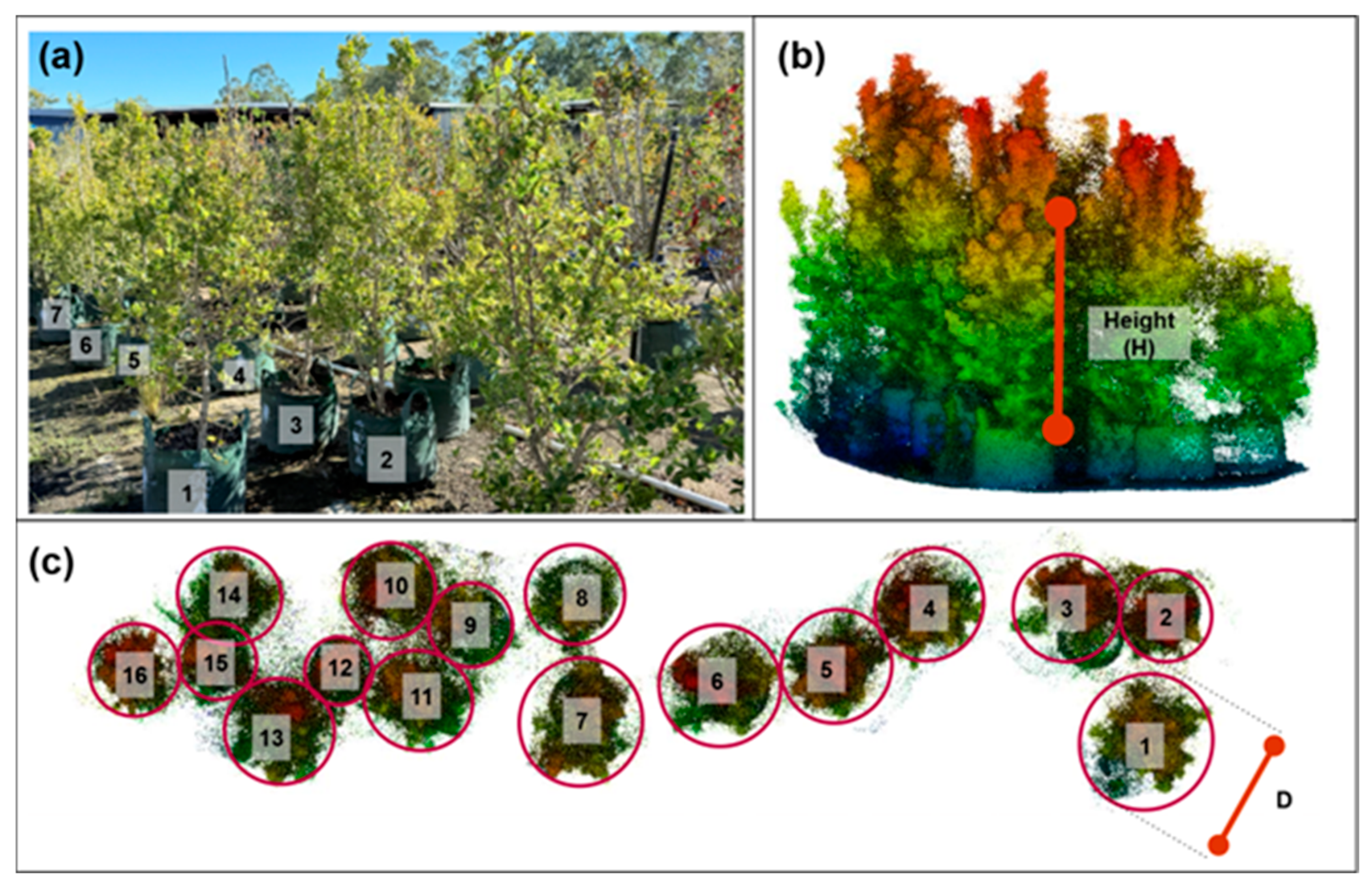
Figure 4. Region containing Lilly Pilly vegetation: (a) Close-up view showing Lilly Pilly vegetations with assigned identification numbers; (b) visualization of individual H measurements using 3D point cloud data; (c) visualization of D for each vegetation with assigned identification numbers.
Remotesensing 17 03454 g004
Figure 5. FDS simulation setup featuring the sensor grid and a sample Lilly Pilly model. The grid indicates the positions of Temperature and Heat Flux sensors placed within the simulation environment.
Remotesensing 17 03454 g005
Figure 6. FDS simulation environment for the sample Lilly Pilly vegetation from the test region.
Remotesensing 17 03454 g006
Figure 7. (a) MS orthomosaic map of the test region; (b) Semantic segmentation map produced by the meta-model where red pixels indicate the Lilly Pilly, white pixels indicate other vegetations, and black pixels indicate non-vegetation region; (c) Watershed-based delineation of Lilly Pilly patches visualized over the MS imagery, where red lines show the patch boundaries.
Remotesensing 17 03454 g007
Figure 8. (a) Vegetation delineation derived from the LiDAR point cloud using RayCloudtools; (b) Projected Instance ID map visualizing individual vegetation segments, where different colors are assigned to different vegetation instances.
Remotesensing 17 03454 g008
Figure 9. Filtering of Lilly Pilly point cloud in the test region: (a) Lilly Pilly patches extracted using the ML-based semantic segmentation model, followed by the watershed algorithm and aligned on the MS imagery; (b) Corresponding filtered LiDAR point cloud instances representing Lilly Pilly vegetation within the defined test region.
Remotesensing 17 03454 g009
Table 1. Summary of selected studies on estimating thermal and fire behavior parameters, highlighting the tools, predicted outputs, input data sources, and key observations.
Predicted/Detected ResponsesModels/Simulation PlatformsPrimary FocusData AcquisitionPlace of StudyRemarksReference
Radiant heat fluxPhysics-based Numerical, WFDS, FDSElevated vegetation in WUIExperimental data and field measurementsUSASimulates fluid flow, combustion, heat transfer and thermal degradation.[7]
Fire behavior for different fuel conditionsCFD modeling and FDSWUIHistorical fire data in SE FranceFranceWUI fire modeling with CFD for different vegetation scenarios (fuel loads) with 3D fire propagation assessment in FDS[20]
Fire spread in grasslandsPhysics-based computer simulation,
WFDS
Grasslands WFDS simulation dataAustraliaPredicts head fire spread rates and fire perimeter development under varying wind and ignition conditions[21]
Fire spread rateA generic, empirical-based modelHeathland
and shrubland
Experimental dataAustraliaDead fuel moisture content is predicted. The model demonstrates rate-of-spread predictions.[22]
Heat transfer in structures (HF and T)CDF modeling and FDSWUI vegetation and building structuresSimulated data
(Lagrangian particle models)
PortugalGoverning parameters in burning vegetation in WUI were quantified in FDS. Impacts were assessed on buildings and quantified heat release rates, HF and T[23]
Heat transfer, AGBPoint cloud-based,
FDS
Woodland surroundingUAS–LiDARAustraliaGeometric features of vegetation components, and foliage incorporated into heat transfer[24]
Heat transferCFD modeling and Point cloud-based, FDSBuilding structures in bush fire prone areasUAV-LiDARAustraliaPoint clouds were utilized to construct heat transfer models in FDS, examining wind velocities, temperature profiles, and pressure distributions during bushfire events.[25]
Fuel loadRandom Forest model and numerical calculationsLongleaf Pine (crown level)LiDAR—ALS, TLSUSAEvaluate the effects of ALS, TLS, and their fusion on crown-level structural and fuel metric modeling.[26]
Wildfire risk assessmentBurn-P3 simulation model, numerical calculationsWildlandMODISGreecePredicted fire effects were first quantified and mapped using a spatial index, then builds the burn probability, fire intensity to evaluate the fire risk[27]
Wildfire risk mitigation within the WUIGeoAI simulationWUILANDFIRE 2020, NASA Socioeconomic DataUSAIncorporates spatial data replicate fire behavior.[28]
Bushfire burn severityRandom Forest, Fuzzy Forest, Boosted Regression Tree, and Extreme Gradient BoostingWildlandMODIS, BARRA dataAustraliaBurn severity index is derived, calculated from pre-fire and postfire imagery. The variables influencing the burn severity have been evaluated.[29]
Forest fire risk (Forest Fire Danger Index)RTDSWildlandHistorical disaster data, MCD64, MODIS, China Surface Climate Daily Data SetChinaThe AHP, the entropy method, and minimal relative entropy theory, a CFFRI was developed to evaluate forest fire risk levels.[30]
MCD14ML: NASA MODIS (Moderate Resolution Imaging Spectroradiometer) data, WFDS: Wildland-Urban Interface Fire Dynamics Simulator, CFD: Computational Fluid Dynamics, FDS: Fire Dynamic Simulator, UAV: Unmanned aerial vehicle, GeoAI: Geospatial artificial intelligence, UAS: Unmanned Arial Systems, AGB: Aboveground biomass, BARRA: Atmospheric high-resolution Regional Reanalysis for Australia, RTDS: Real Time Digital Simulator, AHP: Analytic Hierarchy Process, CFFRI: Composite Forest Fire Risk Index, LSTM: Long Short-Term Memory, ALS: Airborne Laser Scanners, TLS: Terrestrial Laser Scanners, USA: United States of America.
Table 2. Spectral indices and their corresponding equations are used in ensemble model development in addition to the multispectral (MS) bands.
ChannelsSpectral IndicesEquations
SI1NDVI N I R R N I R + R
SI2NDWI G N I R G + N I R
SI3GCI N I R G 1
SI4GLI 2 G R B 2 G + R + B
SI5NDRE N I R R E N I R + R E
Table 3. Recorded structural dimensions of Lilly Pilly vegetations derived from LiDAR point cloud data, including height and diameter measurements across the test area. Where H-Hight and D-crown diameter measurements.
Tree IDH (m)D (m)
10.890.594
21.200.443
31.180.555
40.970.604
51.210.445
61.360.618
71.130.574
80.920.473
90.910.422
100.910.467
111.150.479
121.280.298
131.340.543
141.140.453
151.200.310
161.340.446
Table 4. Summary of the hyperparameter settings used for the base and meta models in the developed EL framework.
HyperparameterBaseMeta
XGBoostLightGBMCatBoostRandom ForestXGBoost
Number of Estimators/Trees700120090001200600
Learning Rate0.10.10.3N/A0.1
Max Depth/depth6−18206
Column Sampling10.8N/Amax_features: ‘sqrt’1
Subsampling/Bagging0.70.8N/AN/A0.7
Specific ParametersN/Anum_leaves: 31
min_data_in_leaf: 10
l2_leaf_reg: 5
random_strength: 1
min_samples_split: 2
min_samples_leaf: 1
N/A
Table 5. Performance metrics of base models (XGBoost, Random Forest, CatBoost, LightGBM) and the meta-model for Lilly Pilly semantic segmentation, evaluated using accuracy, recall, precision, and F1 score.
ModelsAccuracyRecallPrecisionFI Score
Base ModelsXGBoost0.82480.8248
0.7700
0.8279
0.7189
0.8228
0.7435
Random Forest0.74690.7469
0.7283
0.7629
0.6224
0.7403
0.6712
CatBoost0.82080.8208
0.7667
0.8212
0.7242
0.8191
0.7449
LightGBM0.84590.8459
0.7924
0.8490
0.7439
0.8444
0.7674
Meta ModelXGBoost0.84510.8451
0.7898
0.8467
0.7387
0.8439
0.7634
Table 6. Class-wise performance metrics of the meta-model (XGBoost) across all 11 vegetation classes, including accuracy, recall, precision, and F1 score.
SpeciesPixel CountClass IDPrecisionRecallF1 ScoreSupport
Syzygium smithii (Lilly Pilly)64,35900.73850.78980.763412,872
Callistemon viminalis55,42810.96570.97880.97229086
Viburnum odoratissum53,19520.93600.90940.92254439
Solitaire palm51,50030.94800.94450.94635100
Hibbertia scandens49,70940.93840.96570.95185942
Livistona australis47,16750.93950.94620.94287433
Cuprocyparis leylandii44,62560.79750.86600.830426,845
Macadamia integrifolia46,14270.89730.77390.83113229
Hibiscus rosa-sinensis37,67480.83840.72210.77593534
Other vegetation64,35990.87710.58740.70362528
Non-vegetation64,359100.79640.70700.749014,531
Disclaimer/Publisher’s Note: The statements, opinions and data contained in all publications are solely those of the individual author(s) and contributor(s) and not of MDPI and/or the editor(s). MDPI and/or the editor(s) disclaim responsibility for any injury to people or property resulting from any ideas, methods, instructions or products referred to in the content.