Article

Reproduction of Smaller Wildfire Perimeters Observed by Polar-Orbiting Satellites Using ROS Adjustment Factors and Wildfire Spread Simulators

Forest Fire Division, National Institute of Forest Science, Seoul 02455, Republic of Korea
*
Author to whom correspondence should be addressed.
Remote Sens. 2025, 17(16), 2824; https://doi.org/10.3390/rs17162824
Submission received: 12 June 2025 / Revised: 6 August 2025 / Accepted: 12 August 2025 / Published: 14 August 2025

Abstract

While geostationary satellites can provide continuous near-real-time observations, their low spatial resolution makes it difficult to detect small wildfires. Conversely, polar-orbiting satellites are capable of observing small wildfires at high spatial resolution, but can operate only within restricted observation periods. To improve wildfire spread prediction accuracy using polar-orbiting satellite observations, this paper proposes a novel methodology to accurately reproduce wildfire perimeters observed at specific time points by these satellites. The approach employs a wildfire spread simulator combined with a rate of spread (ROS) adjustment factor. The proposed algorithm derives ROS adjustment factors for each fuel model based on differential evolution, achieving up to a 0.4 increase in the Sørensen index when reproducing wildfire perimeter data at given observation times. Incorporating these factors into simulator-based predictions allows comprehensive consideration of external factors affecting wildfire propagation, which have not been sufficiently accounted for in previous methods. Moreover, considering the frequent occurrence of small wildfires in Korea, this study establishes a mapping between major species of trees in Korea and corresponding Fire Behavior Fuel Models (FBFMs). This serves as an example of appropriately matching major species of trees to FBFMs for wildfire spread prediction in countries where FBFMs have not been previously applied. The methodology’s effectiveness is demonstrated using wildfire perimeter data from polar-orbiting satellite observations and ignition points of recent wildfires in Korea. The proposed algorithm is expected to significantly enhance wildfire response by swiftly providing critical information for accurate wildfire spread prediction. This will facilitate prompt and precise countermeasures for small wildfires independent of external conditions such as weather.

1. Introduction

In recent years, the frequency and damage associated with wildfires have increased dramatically. For instance, in California, among the 20 largest wildfires recorded from 1932 to 2024, ten occurred during the 2020s [1]. Furthermore, the Southern California wildfires that occurred in January 2025 resulted in estimated damages of up to $275 billion, significantly surpassing the historical record for damages caused by a single wildfire event [2]. This phenomenon is observed globally, including in South Korea, where the number of wildfire occurrences and the average damaged area during the 2020s have drastically increased compared to the period before the 2010s [3]. To mitigate the escalating losses caused by wildfires, one of the most critical measures is preparation in advance against wildfire spread prior to the actual event. Essential to this proactive approach is the accurate prediction of wildfire spread. However, wildfire spread prediction involves highly complex processes, and various dedicated simulators have been developed to address this complexity, including FARSITE and PROMETHEUS [4,5].
In practice, when wildfire spread simulators are executed and the wildfire perimeter is predicted using only meteorological and environmental data, significant discrepancies frequently arise compared to actual wildfire spread results. These discrepancies occur due to various factors. The most significant reason, highlighted by Rothermel et al., is that even when all meteorological and environmental data utilized in simulators are accurate, the theoretically predicted rate of spread (ROS) often deviates substantially from the actual ROS [6]. Additionally, because real-time updating of fuel characteristics utilized in wildfire spread simulations is challenging, discrepancies between the actual fuel conditions and those implemented in simulators sometimes occur, resulting in substantial prediction errors. Consequently, such diverse factors continuously cause differences between predicted and actual wildfire spread results, and these errors progressively accumulate as predictions proceed, rendering accurate wildfire spread prediction increasingly difficult.
To overcome these limitations, actual wildfire perimeter data observed during wildfire spread can be utilized. Numerous studies have been conducted to enhance wildfire spread prediction accuracy by leveraging observed perimeter data. Representative examples include studies directly adjusting the wildfire perimeter using the Ensemble Kalman Filter (EnKF), and studies indirectly correcting the perimeter by optimizing the ROS [7]. EnKF, a Bayesian filter optimized for highly nonlinear systems, has been extensively adopted as a primary method for directly correcting predicted wildfire perimeters. The first application of EnKF to wildfire perimeter prediction was conducted by Mandel et al. [8]. Subsequently, various modified EnKF methods optimized to enhance wildfire spread prediction accuracy have been proposed and applied. These include the Fast Fourier Transform-based EnKF, Polynomial Chaos surrogate model-based EnKF, Ensemble Transform Kalman Filter, and Deterministic EnKF [9,10,11,12].
Studies indirectly correcting wildfire perimeters through the optimization of the ROS have gained significant attention in recent years and have been actively conducted. These studies can be broadly categorized into two groups: those directly deriving ROS, and those optimizing parameters associated with ROS. Research focused on directly deriving ROS was performed by Khanmohammadi et al., who employed various machine learning methods [13]. Furthermore, Cardil et al. rapidly estimated ROS for large wildfires using the Visible Infrared Imaging Radiometer Suite [14]. Studies dedicated to optimizing parameters associated with ROS include Pereira et al. (2022, 2024), who calibrated the wildfire spread model parameters proposed by Rothermel [15,16,17]. Additionally, Srivas et al., Zhou et al., and Yoo et al. conducted studies utilizing diverse methodologies and observational data to optimize the ROS adjustment factor introduced in FARSITE [18,19,20]. Typically, the ROS adjustment factor assigns values based on fuel models classified according to the Fire Behavior Fuel Models (FBFM) suggested by Anderson or Scott [21,22]. However, the classification of fuel models based on FBFM is limited to only a few countries, including the United States. In many countries with increasing wildfire occurrences, such as South Korea, only data on the species of trees is generally available, making it challenging to apply the ROS adjustment factor due to the lack of FBFM-based classification data.
Meanwhile, aerial monitoring, including drones, airborne imaging systems, and various satellites, has recently been the most commonly used method for collecting actual wildfire perimeter observation data [23]. The advantages and disadvantages of each aerial data collection tool are summarized in Table 1. Among these tools, geostationary satellites are capable of continuous and near-real-time monitoring with minimal external environmental constraints. Studies utilizing geostationary satellite observation data to derive ROS and ROS adjustment factors have been conducted by Liu et al. and Yoo et al. [24,25]. However, due to their high orbital altitudes, geostationary satellites suffer from extremely low spatial resolution; even the latest geostationary satellites, such as Himawari-8 and GOES-R, have spatial resolutions limited to approximately 2 km × 2 km [26,27]. As a result, in countries with smaller land areas and frequent small-scale wildfires, such as South Korea, the practical utility of geostationary satellite observation data is limited.
Among the high-resolution data collection tools required in such situations, polar-orbiting satellites are the least affected by external environmental constraints. However, they can only collect data for brief periods, which makes continuous real-time data acquisition unfeasible. Therefore, research aimed at improving wildfire spread prediction accuracy using polar-orbiting satellite observation data should focus on enhancing prediction accuracy based on a single perimeter observation at a specific time. This is preferable to attempting real-time updates using continuous time-series data. However, previous studies related to improving wildfire prediction accuracy by deriving and adjusting relevant parameters have been limited to those utilizing wildfire perimeter data collected over consecutive time steps [28]. Research focusing solely on using single-instance perimeter observations for parameter derivation and adjustment has not yet been conducted.
This paper first introduce a criterion for matching fuel models with dominant species of trees in South Korea, a country where FBFM has not previously been applied. If each tree species classified in Korea’s forest type map is individually assigned a separate fuel model, the number of fuel models becomes excessively large compared to the widely used FBFM proposed by Anderson [21]. Therefore, similar species of trees were grouped into the same fuel model, resulting in an FBFM consisting of nine fuel models in total. Subsequently, this paper proposes a methodology for deriving the ROS adjustment factor for each fuel model, allowing a wildfire spread simulator to reproduce observed wildfire perimeters collected through polar-orbiting satellites with improved accuracy. In this methodology, an optimized wildfire spread simulator tailored for Korean environmental conditions, previously developed by Lee et al., is employed alongside differential evolution (DE) to determine optimal ROS adjustment factors [29,30]. By applying the derived ROS adjustment factors to simulator-based spread predictions beyond the wildfire perimeter observation time, previously unaccounted external factors influencing wildfire spread can be effectively integrated. This application significantly enhances prediction accuracy.
In the following section (Section 2), we describe existing FBFMs proposed and utilized internationally, and then suggest corresponding criteria for applying FBFM-based ROS adjustment factors in South Korea. Section 3 proposes a detailed methodology using FBFM and DE to derive ROS adjustment factors, based on actual observed wildfire perimeter data at a specific time. Section 4 applies the proposed methodology to various real wildfire cases in South Korea using polar-orbiting satellite observation data, and evaluates its performance by comparing simulator-based wildfire spread prediction results. Lastly, Section 5 provides a summary and suggestions for future research topics.

2. Grouping Tree Species into Fuel Models with Similar Fire Behavior

2.1. Fire Behavior Fuel Models

In wildfire spread modeling, fuel refers to combustible materials present on the ground surface, such as grasses, shrubs, and litter. Since the physical and chemical properties of fuel significantly influence wildfire behavior, a fuel classification system known as the FBFM was developed to predefine representative properties for various fuel types. These representative properties are then used as input parameters in mathematical wildfire spread models, such as the one proposed by Rothermel [17]. Each FBFM defines key characteristics in advance, including fuel load, fuel depth, surface-area-to-volume ratio, dry bulk density, heat content, and moisture content of extinction. These properties are then used in wildfire spread prediction simulators such as FARSITE and PROMETHEUS to compute various fire behavior metrics, including wildfire ROS, perimeter, flame length, and heat per unit area [4,5]. The use of FBFMs offers several advantages: (1) the use of standardized fuel models facilitates consistent comparison of results across different studies and institutions; (2) it provides a systematic guide for prioritizing variable measurements during field surveys; and (3) it enables the analysis of discrepancies between simulation results and observed fire behavior using fuel characteristics as a basis.
Representative examples of FBFMs include the model developed by Anderson, which comprises 13 fuel types, and the model developed by Scott and Burgan, which consists of 40 fuel types [21,22]. Anderson’s FBFM is a static fuel model, defining fixed fuel characteristics based on specific assumptions regarding time, season, and moisture conditions. The list of fuel models included in Anderson’s classification is presented in Table 2. While this model is simple to use, it has the limitation of not reflecting seasonal or weather-related changes in fuel conditions. In contrast, the FBFM proposed by Scott and Burgan is a dynamic fuel model that accounts for variations in fuel properties based on temperature, humidity, and seasonal changes. However, because this model requires more fine-grained classification criteria than tree species, it may not be suitable for application in countries where FBFMs have not previously been applied.

2.2. Fuel Model Classification and Mapping for Major Tree Species in South Korea

This section proposes a fuel model classification and mapping based on the forest type map for South Korea, where FBFMs have not previously been applied. In addition to the advantages of using FBFMs described in Section 2.1, this process was carried out to enable the application of ROS adjustment factors based on FBFMs when running wildfire spread simulators. The classification and mapping were conducted using the 5th Forest Type Map provided by the Korea Forest Service, which contains various data fields including stand origin, forest type, tree species, diameter at breast height class, age class, and crown density [31]. Among these, the information utilized in this study was limited to age class and tree species, which are described in detail in Table 3. The use of only these two variables in this study is that, in the ROS calculation formula proposed in [17] and applied in [29], the relevant factors are influenced solely by these two variables.
First, the fuel models for coniferous forests, broadleaf forests, and mixed forests must be distinguished, as Anderson assigned different fuel models to broadleaf species and coniferous species [21]. In this study, species that occupy large areas in South Korea were each assigned to a unique fuel model, while those occupying smaller areas were grouped together under a single fuel model. A major limitation in the South Korean context is that experimentally measured values for key fuel characteristics—such as fuel load, fuel depth, and surface-area-to-volume ratio, which are required for the wildfire spread model proposed by Rothermel—are available for only a limited number of species [17]. These species include Korean red pine, Korean pine, Japanese larch, Pitch pine, and Black pine, which are predominant across the country; therefore, each of them was assigned a separate fuel model. Regarding age class, although different fuel models were not assigned to different age classes within the same species, age-specific values were applied for the relevant fuel characteristics. Based on these considerations, tree species were ultimately classified into fuel models as summarized in Table 4.
The characteristic values used for the wildfire spread model were primarily based on the Korea Forest Service [32]. Among these, the dry bulk density, heat content, and moisture content of extinction—parameters with minimal or difficult-to-quantify effects on fire behavior—were assumed constant across all fuel models: 512.71 kg/m3, 18,607.112 kJ/kg, and 0.3, respectively [17,33]. In contrast, fuel load, fuel depth, and surface-area-to-volume ratio varied by fuel model and age class, and are also presented in Table 4.

3. ROS Adjustment Factor Derivation for Reproducing Wildfire Perimeters Observed by Polar-Orbiting Satellites

3.1. Differential Evolution-Based ROS Adjustment Factor Derivation Algorithm

Polar-orbiting satellites provide high-resolution observations of wildfire perimeters, but unlike geostationary satellites, they cannot continuously monitor a specific location, resulting in significant intervals between subsequent observations. For instance, the MODIS sensor operating on NASA’s Terra satellite revisits a specific location every 1–2 days, Sentinel-2 every 5 days (at the equator), and Landsat 8 every 16 days [34]. Therefore, to effectively utilize high-resolution observations from polar-orbiting satellites, it is essential to identify methods that improve wildfire spread prediction accuracy by integrating wildfire perimeter data observed at a specific time with wildfire spread simulation models.
In this study, a ROS adjustment factor is introduced into wildfire spread simulations to comprehensively account for factors that significantly influence actual wildfire propagation but cannot be explicitly included in current simulation models. Such factors include transient vegetation dryness due to sudden decreases in precipitation, increased wildfire fuel loads from widespread tree mortality caused by diseases, and unpredictable localized strong winds or gusts. The ROS adjustment factor is derived using DE to ensure that the wildfire spread simulator closely reproduces the observed wildfire perimeter at a specific point in time. Consequently, this ROS adjustment factor consolidates all wildfire spread influences up to that specific time that cannot be explicitly accounted for in the existing spread simulator into a single factor. By applying the derived ROS adjustment factor to subsequent wildfire spread predictions, these influencing factors can continue to be considered. This approach is particularly effective for smaller wildfires, where environmental conditions within areas already affected by wildfire are likely similar to those in regions expected to spread subsequently. The proposed DE-based algorithm for deriving the ROS adjustment factor is outlined as follows:
[Step 1]
Upon wildfire ignition, the following data required for running the wildfire spread simulation are collected in advance:
Terrain and fuel-related variables, including elevation, slope, aspect, fuel model, stand height, canopy cover, canopy base height, canopy bulk density, and foliar moisture content
Weather-related variables consist of temperature, relative humidity, hourly precipitation amount, wind speed and direction, fuel moisture, and cloud cover percentage
Estimated ignition point location (primarily based on the reported location, but terrain, fuel, and weather variables may also inform the estimation)
[Step 2]
When a polar-orbiting satellite passes over the wildfire area, obtain wildfire perimeter and burned area observation data.
[Step 3]
DE Initialization: An initial population of ROS adjustment factors is generated, consisting of N vectors of dimension n : x 1 ,   x 2 ,   ,   x N ,   x i = x i 1 , x i 2 ,   ,   x i n R n . Here, N denotes the population size, and n is the number of elements in the ROS adjustment factor. A discussion on the appropriate choice of N is provided in Section 3.2.
[Step 4]
The objective function f is defined as:
f x i = 1 S I A , B = 1 2 A B A + B
where S I denotes the Sørensen index, A is the burned area observed by the polar-orbiting satellite in Step 2, and B is the predicted burned area produced by the wildfire spread simulation using the ROS adjustment factor x i [35].
[Step 5]
The best solution from the current population is selected as x b e s t = a r g m i n x x 1 ,   ,   x N f x . Then, Steps 6 through 8 are applied to each x i , for i 1 ,   2 ,   ,   N .
[Step 6]
DE Mutation: Randomly select two individuals x r 1 and x r 2 from the population, and compute the mutant vector v i = x b e s t + F x r 1 x r 2 where F is the differential weight. The selection of an appropriate value for F is discussed in Section 3.2.
[Step 7]
DE Crossover: Given vectors x i = x i 1 , x i 2 ,   ,   x i n and v i = v i 1 , v i 2 ,   ,   v i n , a trial vector u i = u i 1 , u i 2 ,   ,   u i n is generated as follows:
u i j = v i j ,    i f   r a n d 0 , 1 < C R x i j ,    o t h e r w i s e                
This process is independently applied for each index j 1 ,   2 ,   ,   n . That is, each element of the trial vector u i is selected from the mutant vector v i with probability C R , or from the original vector x i with probability 1 C R . The parameter C R denotes the crossover probability. A detailed discussion of appropriate values for C R is provided in Section 3.2.
[Step 8]
DE Selection: If the trial vector u i has a better objective function value than x i , i.e., if f u i < f x i , then x i is replaced by u i . Whether replacement occurs or not, the result is denoted as x i .
[Step 9]
If the updated population x 1 ,   x 2 ,   ,   x N satisfies the stopping criterion, the algorithm proceeds to Step 10. Otherwise, the updated population is used as the new population, and the process returns to Step 5. The stopping condition is defined as:
S s t d f x i t o l × m e a n f x i
where t o l is a predefined coefficient used to determine whether the population has sufficiently converged, by evaluating the standard deviation of fitness values relative to their mean. The optimal value of t o l can vary substantially depending on the wildfire spread prediction results, the characteristics of the objective function, and the structure of the solution space. Consequently, it should be selected based on empirical tuning appropriate to the problem context.
[Step 10]
Once the stopping criterion is met, the final ROS adjustment factor is selected by applying the same procedure as in Step 5 to the final population. The selected optimal ROS adjustment factor is then used in subsequent wildfire spread simulations.
Figure 1 presents the flowchart of the DE-based algorithm proposed in this paper for estimating ROS adjustment factors to reproduce wildfire perimeters observed by polar-orbiting satellites.

3.2. Considerations in Implementing the Proposed Algorithm

Various global optimization methods can be applied to derive the optimal ROS adjustment factor. Besides DE used in the proposed algorithm, Genetic Algorithm (GA) and Particle Swarm Optimization (PSO) are also widely adopted global optimization techniques. GA is suitable for optimization problems with discontinuous solution spaces and allows a variety of solution representations; however, it has disadvantages such as slow convergence speed and high computational cost when applied to continuous solution spaces [36]. In contrast, DE and PSO exhibit significantly faster convergence in continuous solution spaces compared to GA, making them more suitable for ROS adjustment factor optimization. Specifically, PSO generally demonstrates faster convergence speed, whereas DE achieves higher optimization accuracy [37]. In this study, DE was chosen for deriving the optimal ROS adjustment factor. However, if the priority is convergence speed rather than accuracy, employing PSO is also a viable option.
In the proposed algorithm, the performance in terms of convergence speed and accuracy depends heavily on the selection of DE parameters, including the population size N , differential weight F , and crossover probability C R . Regarding the population size, if N is too small, the algorithm may lack diversity in the search space, increasing the risk of falling into local minima. Conversely, an excessively large N substantially increases computational costs. Storn and Price, who originally proposed DE, recommended choosing N within the range 5 n < N < 10 n [30]. Subsequent research has extensively explored appropriate choices of N , investigating cases ranging from very small populations ( N n ) to considerably large populations ( N 40 n ), as well as employing adaptive or variable N strategies. Piotrowski compared outcomes across various n , finding that, for cases such as the FBFM scenario—with dimensionality n 10 —, the most efficient results were obtained at population sizes of N = 5 n or N = 10 n , excluding relatively understudied adaptive N methods [38].
For the differential weight F , values between 0.4 and 1.0 are generally recommended, with a suggested default of 0.5 . Selecting a differential weight value that is too large risks causing algorithm divergence, while a value that is too small may cause premature convergence to local minima. As for the crossover probability C R , typical recommendations are 0.9 for global DE variants and 0.1 for local DE variants. A higher crossover probability allows a broader exploration of the solution space during the early optimization stages, whereas a lower crossover probability can achieve more precise convergence in later stages. Numerous studies have also explored the optimal selection of F and C R across various problems. In particular, research involving adaptive or variable F and C R has been conducted extensively, surpassing the scope of studies on adaptive population sizes [39]. As a result of these studies, most current DE implementations and libraries commonly use default values of F = 0.8 or F ~ U n i f o r m 0.5 ,   1.0 , and C R = 0.9 .

4. Numerical Investigations

4.1. Description of Observation and Input Data Used for Algorithm Validation

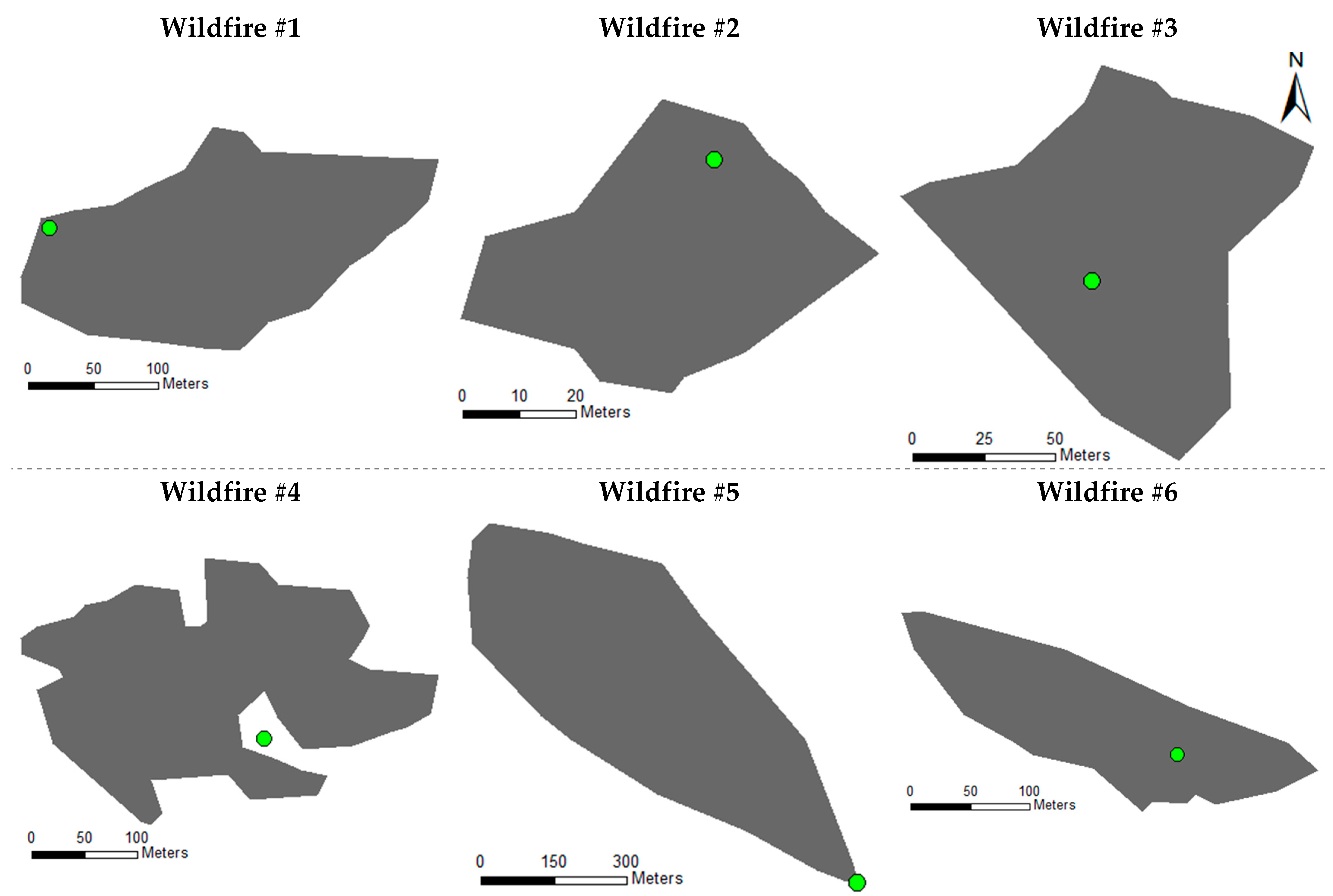
To verify the effectiveness of the proposed methodology and algorithm, this study utilized data from six small or medium-scale wildfire cases that occurred in South Korea. Detailed information for each wildfire case is presented in Table 5. Over 80% of the damage area for wildfire consists of nine tree species corresponding to fuel models 1, 2, 3, 4, 5, and 7. This indicates that the approach used to map Korean tree species to fuel models, as presented in Table 4, is reasonable. It should be noted that the entire duration and area of wildfire spread were not fully utilized when validating the proposed algorithm. Almost all current wildfire spread prediction simulators assume wildfire propagation without suppression activities; however, in reality, firefighting operations typically begin immediately after the wildfire is detected in its early stages. Due to such early firefighting interventions, validation of wildfire spread prediction algorithms becomes challenging, as data from wildfires subjected to active suppression are unsuitable. For accurate verification of prediction accuracy, wildfire data with little to no suppression activities are required. Wildfires that spread significantly without early suppression efforts are rare and occur under specific circumstances, such as wildfires ignited naturally deep within mountainous terrain or simultaneous multiple wildfire events. In the former case, significant time may elapse before ground wildfire monitoring personnel discover the wildfire or smoke, especially in locations without nearby roads accessible by humans. In the latter case, due to the shortage of firefighters and firefighting equipment, firefighting resources must be concentrated on wildfires predicted to cause greater damage, inevitably leaving some wildfires unsuppressed. The wildfires described in Table 5 represent cases in which firefighting activities were minimal or absent until the wildfire damage area and perimeters were observed by polar-orbiting satellites. Thus, the proposed methodology validation employs data up to the time of satellite observation. Figure 2 presents the wildfire-affected areas at the time of polar-orbiting satellite observation for each wildfire, and ignition point locations. In the case of wildfire No. 4, the ignition point appears to be located outside the wildfire-affected area. This discrepancy could be attributed either to errors in the satellite observation data or inaccuracies in the ignition point identification. However, as both types of errors could realistically occur in wildfire scenarios, the validation proceeded without further adjustment or correction of the wildfire perimeters or ignition point positions.
The wildfire spread simulator used for validating the proposed methodology was the Korean wildfire spread simulator proposed by Lee et al. [29]. The simulator was configured with a spatial resolution of 5 m and a temporal resolution of 3 min. The FBFM employed in this section was the model proposed in Section 2.2 of this paper. The upper bound of the ROS adjustment factor was set to 5.0 and the lower bound to 0.1 during the algorithm implementation. The lower bound of 0.1 corresponds to cases where the wildfire scarcely spreads for a particular fuel model due to certain reasons. The upper bound was chosen such that no ROS adjustment factor values would actually reach this limit during the analysis. The three parameters mentioned in Section 3.2—population size N , differential weight F , and crossover probability C R —were set as N = 50 , F ~ U n i f o r m 0.5 ,   1.0 , and C R = 0.9 , respectively. The value of t o l in Equation (3) was fixed at 0.01 for all experiments. Among the data described in Step 1 of Section 3.1, weather-related variables were obtained from the Korea Meteorological Administration, whereas terrain and fuel-related variables were sourced from the Korea Forest Research Institute and the National Geographic Information Institute [31,40,41].

4.2. Derived ROS Adjustment Factors and Accuracy Comparison of Wildfire Spread Predictions

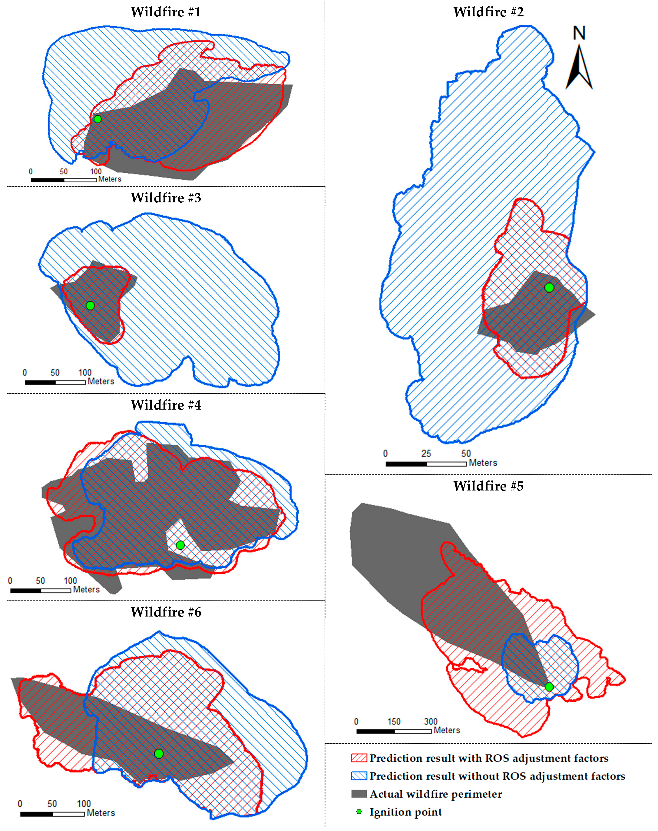
Table 6 presents the ROS adjustment factors derived for each wildfire using the proposed methodology, along with the corresponding Sørensen indices for the wildfire spread prediction results. The gray cells indicate cases where no area corresponding to the respective fuel model existed within the spread region of a given wildfire. In such cases, the ROS adjustment factor did not influence the simulation results and was therefore excluded from the optimization process performed using DE. For comparison, the Sørensen indices of the wildfire spread predictions without applying ROS adjustment factors are also provided. In addition, Figure 3 visually compares the wildfire spread prediction results—both with and without the ROS adjustment factors listed in Table 6—against the actual wildfire perimeters.
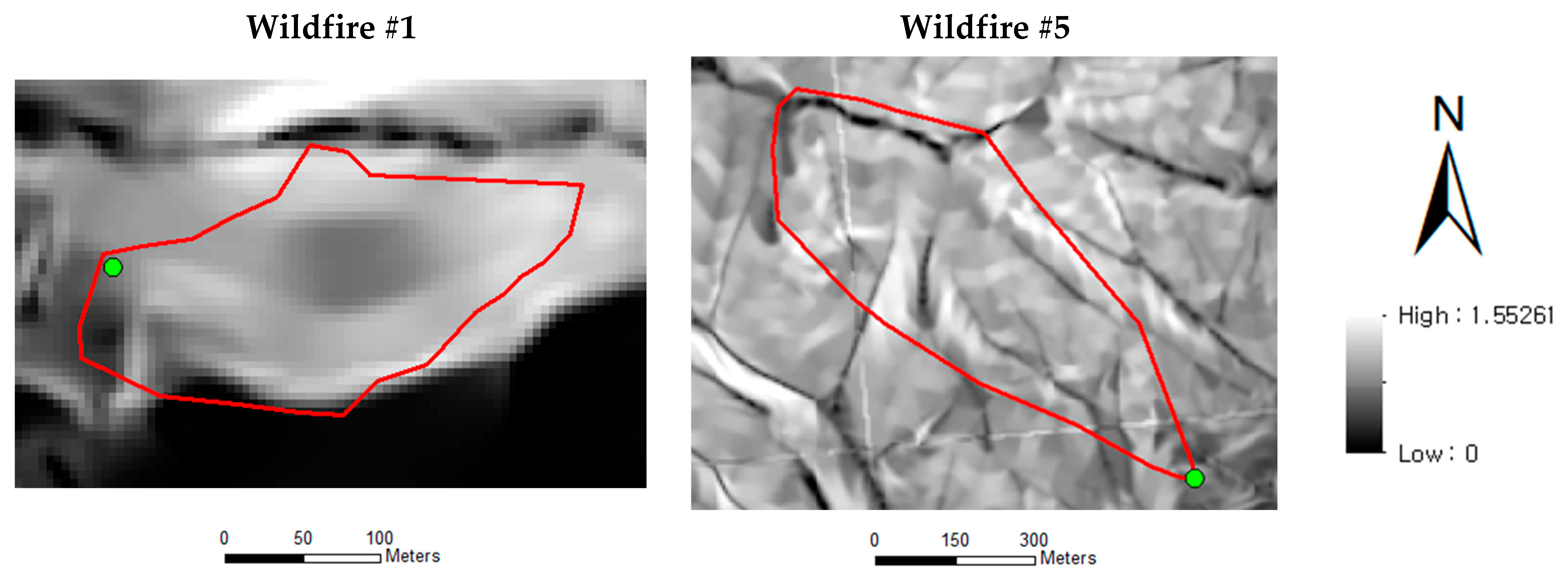
Situations in which the ROS adjustment factor approached the lower bound of 0.1 occurred multiple times, whereas cases where it approached the upper bound of 5.0 were observed only for fuel model 0 in Wildfire #1 and fuel model 7 in Wildfire #5. Several factors can lead to situations where the ROS adjustment factor approaches the lower bound. For example, if the fuel in a particular fuel model is saturated, or if the proportion of live fuel is significantly higher, wildfire spread may take considerably longer. In addition, changes in the vegetation structure within a fuel model can block wind or create turbulence, resulting in a sharp reduction in the ROS. For fuel models corresponding to such conditions, the ROS adjustment factor could be further reduced if the lower bound were set below 0.1. However, as situations where wildfire spread completely stops after a fuel model transition are uncommon, the lower bound was set at 0.1. Cases where the ROS adjustment factor approached the upper bound are generally assumed to be strongly influenced by topography. When the slope in a given area is steep, the wildfire can spread much faster than the predicted ROS, leading to very high ROS adjustment factor values. In fact, an examination of the slope in the spread areas of Wildfires #1 and #5 confirmed that the slope exceeded 40 degrees (approximately 0.7 radian) in almost all areas. The slope plots for the spread areas of these two wildfires are presented in Figure 4.
In all cases, the wildfire spread predictions obtained using the proposed algorithm and derived ROS adjustment factors produced results significantly closer to actual wildfire perimeters. Wildfire #3 exhibited the most substantial improvement, where applying the ROS adjustment factor drastically increased the Sørensen index from 0.213 to 0.896. Comparing the shape of wildfire perimeters revealed that, in directions other than the left side relative to the ignition point, the wildfire spread area was significantly overestimated without applying the ROS adjustment factor. However, when the proposed methodology and ROS adjustment factor were applied, the predicted areas significantly decreased and closely aligned with the actual perimeters. On the left side, where the prediction was relatively accurate even without applying the ROS adjustment factor, the application of the factor maintained a similar predicted area while slightly increasing detailed accuracy. This indicates that the adjustment of wildfire spread predictions using ROS adjustment factors can be applied differently according to locations and directions, effectively addressing diverse real wildfire perimeters. Through this process, the final prediction accuracy improved dramatically.
Similar to wildfire #3, wildfire #1 also showed a significant increase in the Sørensen index from 0.366 to 0.786. Unlike wildfire #3, wildfire #1 had areas that were both overestimated (upper left) and underestimated (lower right). By individually adjusting the predicted spread areas for each direction using ROS adjustment factors, the final predicted perimeter closely matched the actual perimeter in both directions. Wildfire #4 also exhibited a high Sørensen index of 0.821 upon applying the proposed methodology and ROS adjustment factors; however, since the prediction accuracy without applying the ROS adjustment factors was already relatively high, with a Sørensen index of 0.734, the index did not increase dramatically. Nonetheless, the validation demonstrated that, even when the prediction accuracy without applying ROS adjustment factors was already relatively high, appropriate adjustment of the factors could further improve the accuracy of detailed predictions. In this case, the adjustments corrected slight overestimations in the upper-right area and slight underestimations on the left side.
For wildfires #2, #5, and #6, relatively lower Sørensen index values ranging from 0.471 to 0.591 were obtained, even when applying the proposed algorithm and ROS adjustment factors, compared to the previous wildfires. A common characteristic of wildfires #2 and #5 was their very low Sørensen index values without applying ROS adjustment factors, being 0.162 and 0.145, respectively. Due to these low initial values, even after applying ROS adjustment factors, their prediction accuracy could not reach the higher levels observed for wildfires #1, #3, and #4. Still, the differences in Sørensen indices before and after applying ROS adjustment factors were substantial, at 0.389 and 0.326, respectively, demonstrating meaningful improvements in accuracy. For wildfire #6, applying ROS adjustment factors significantly improved the accuracy of the left side, which had previously been underestimated, resulting in predictions closely matching the actual perimeter. However, the right side, initially overestimated without ROS adjustment factors, showed reduced overestimation after applying the factors but was still noticeably overestimated, which limited the overall increase in the Sørensen index. Nevertheless, the proposed methodology demonstrated meaningful improvements across all wildfires tested, albeit with varying degrees of effectiveness.

4.3. Limitations and Outlook

This study aimed to represent the impacts of various factors affecting wildfire spread, particularly those difficult to incorporate into wildfire spread simulators due to challenges in data collection or quantification, or that are not supported by existing simulation models. These impacts were expressed through a single parameter, the ROS adjustment factor, derived from wildfire perimeter data observed by polar-orbiting satellites at specific time points. It was anticipated that applying the derived ROS adjustment factor within the wildfire spread simulator, up to the satellite observation time, would enable highly accurate reproduction of the wildfire perimeter data captured by the polar-orbiting satellites. Furthermore, applying this factor in simulations beyond the observation time was expected to improve the prediction accuracy by incorporating previously unaccounted factors into the spread prediction.
Validation of the proposed methodology demonstrated that applying the derived ROS adjustment factor significantly improved the simulator’s ability to reproduce the wildfire perimeter data observed by polar-orbiting satellites at the specific observation time. However, verifying the effectiveness of the ROS adjustment factor for predictions beyond the satellite observation time was hindered by the lack of suitable real wildfire datasets. This is due to wildfire spread simulators generally not accounting for firefighting interventions. Since firefighting operations usually begin immediately after wildfire detection, datasets where firefighting activities were not conducted between two separate observations by polar-orbiting satellites are virtually nonexistent. To overcome this limitation, further validation of the methodology requires one of the following conditions: (1) utilizing multiple polar-orbiting satellites to collect suitable wildfire datasets for algorithm validation, or (2) developing methods to incorporate firefighting effects into wildfire spread simulators and refining the proposed algorithm accordingly. Further validation will therefore depend on meeting at least one of these conditions.
The validation results discussed in Section 4.1 and Section 4.2 revealed that for wildfires where prediction accuracy was extremely low without the ROS adjustment factors—specifically, wildfires #2, #5, and #6—the improvements after applying the proposed methodology and ROS adjustment factors were limited. One solution to address this issue is to subdivide fuel models within the FBFM. By dividing areas currently represented by a single fuel model into multiple distinct fuel models, more diverse and realistic wildfire perimeter shapes can be generated in simulations. As seen in the United States, Anderson’s 13 fuel models and the expanded 40 fuel models by Scott and Burgan have been successfully implemented. Similarly, countries that currently use fewer fuel models in their FBFMs, such as South Korea, may eventually adopt more detailed FBFMs with a larger number of fuel models once a stable application of the existing system is achieved. However, this requires not only the data already available in forest type maps but also more diverse fuel-related data, which necessitates additional data collection before future research can proceed. Another potential solution for overcoming these accuracy limitations includes applying the directional ROS adjustment factor proposed by Yoo et al., a method that also warrants further exploration in subsequent studies [20].

5. Conclusions

In this study, a novel methodology was proposed that combines a wildfire spread simulator, a rate of spread (ROS) adjustment factor, and differential evolution (DE) to accurately reproduce the spread of small-scale wildfires as observed with high precision by polar-orbiting satellites. Since polar-orbiting satellites can only collect data at most once or twice per day, the temporal resolution is limited, making it crucial to improve the accuracy of spread predictions between observation times. To address this, the proposed algorithm derives the ROS adjustment factors for each fuel model using DE, such that the wildfire spread simulator produces results that closely match the wildfire perimeters observed at the given time. Furthermore, most countries where small-scale wildfires are predominant have not previously applied FBFMs. To address this, this study constructed an FBFM consisting of nine fuel models by grouping major tree species in South Korea—an example of such a country—based on species similarity. This facilitates the application of the ROS adjustment factor and the proposed algorithm.
To validate the proposed methodology, numerical investigations were conducted on six recent small wildfire cases in South Korea. The ROS adjustment factors derived through the proposed algorithm enabled significantly more accurate reproduction of the actual wildfire perimeters using the wildfire spread simulator under the given environmental conditions and the newly constructed Korean FBFM. This improvement was confirmed through comparisons based on the Sørensen index. In cases where the predictions without ROS adjustment factors yielded completely different results from the actual wildfire perimeters, applying the ROS adjustment factor improved the Sørensen index to around 0.47 or higher, resulting in a moderately similar prediction. In cases where a certain level of accuracy was already present without applying the ROS adjustment factor, applying it further improved the Sørensen index to up to approximately 0.9, indicating highly accurate predictions.
The proposed methodology approximates the effects of various external factors—typically not integrated into conventional wildfire simulators—by incorporating them into a single ROS adjustment factor. This enables continued wildfire spread prediction even after the time of polar-orbiting satellite observation. Such an approach is especially effective in small wildfire scenarios, where environmental conditions affecting wildfire spread are likely to remain consistent between the observed and subsequent spread areas. However, to clearly validate this aspect, wildfire data are required in which polar-orbiting satellites observe the same wildfire more than once without wildfire suppression activities occurring. When using only a single polar-orbiting satellite, obtaining such data is challenging. Therefore, future studies should aim to collect suitable wildfire datasets using multiple polar-orbiting satellites and conduct further validation of the proposed methodology. Alternatively, the development of wildfire spread prediction algorithms that can incorporate the effects of suppression activities would also help supplement the validation of the methodology.

Author Contributions

Conceptualization, S.Y. and S.C.; methodology, S.Y.; software, S.Y. and S.C.; validation, S.Y., C.K. and S.C.; formal analysis, S.Y. and S.C.; investigation, S.Y. and S.C.; resources, C.K. and S.C.; data curation, S.Y. and S.C.; writing—original draft preparation, S.Y.; writing—review and editing, S.C.; visualization, S.Y. and S.C.; supervision, S.C.; project administration, C.K. and S.C.; funding acquisition, S.C. All authors have read and agreed to the published version of the manuscript.

Funding

This study was conducted as part of a research project (FE0100-2023-03-2025) supported by the National Institute of Forest Science.

Data Availability Statement

The raw data supporting the conclusions of this article will be made available by the authors on request.

Acknowledgments

This research was supported by the Korea Forest Service through the R&D project (RS-2024-00402509).

Conflicts of Interest

The authors declare no conflicts of interest.

Abbreviations

The following abbreviations are used in this manuscript:
ROSRate of Spread
FBFMFire Behavior Fuel Model
EnKFEnsemble Kalman Filter
DEDifferential Evolution
GAGenetic Algorithm
PSOParticle Swarm Optimization

References

  1. CAL FIRE. Top 20 Largest California Wildfires. Available online: https://fire.ca.gov/our-impact/statistics (accessed on 11 March 2025).
  2. AccuWeather. AccuWeather Estimates More Than $250 Billion in Damages and Economic Loss from LA Wildfires. Available online: https://www.accuweather.com/en/weather-news/accuweather-estimates-more-than-250-billion-in-damages-and-economic-loss-from-la-wildfires/1733821 (accessed on 11 March 2025).
  3. Chang, D.Y.; Jeong, S.; Park, C.E.; Park, H.; Shin, J.; Bae, Y.; Park, H.; Park, C.R. Unprecedented wildfires in Korea: Historical evidence of increasing wildfire activity due to climate change. Agric. For. Meteorol. 2024, 348, 109920. [Google Scholar] [CrossRef]
  4. Finney, M.A. FARSITE, Fire Area Simulator—Model Development and Evaluation; No. 4; USDA Forest Service, Rocky Mountain Research Station: Ogden, UT, USA, 1998.
  5. Tymstra, C.; Bryce, R.W.; Wotton, B.M.; Taylor, S.W.; Armitage, O.B. Development and Structure of Prometheus: The Canadian Wildland Fire Growth Simulation Model; Information Report. NOR-X-417; Natural Resources Canada, Canadian Forest Service, Northern Forestry Centre: Edmonton, AB, Canada, 2010.
  6. Rothermel, R.C.; Rinehart, G.C. Field Procedures for Verification and Adjustment of Fire Behavior Predictions; General Technical Report INT-142; USDA Forest Service: Ogden, UT, USA, 1983.
  7. Evensen, G. Data Assimilation: The Ensemble Kalman Filter, 2nd ed.; Springer Science & Business Media: Berlin/Heidelberg, Germany, 2009. [Google Scholar]
  8. Mandel, J.; Bennethum, L.S.; Beezley, J.D.; Coen, J.L.; Douglas, C.C.; Kim, M.; Vodacek, A. A wildland fire model with data assimilation. Math. Comput. Simul. 2008, 79, 584–606. [Google Scholar] [CrossRef]
  9. Mandel, J.; Beezley, J.D.; Kondratenko, V.Y. Fast Fourier transform ensemble Kalman filter with application to a coupled atmosphere-wildland fire model. In Computational Intelligence in Business and Economics; World Scientific: Singapore, 2010; pp. 777–784. [Google Scholar]
  10. Rochoux, M.C.; Ricci, S.; Lucor, D.; Cuenot, B.; Trouvé, A. Towards predictive data-driven simulations of wildfire spread–Part I: Reduced-cost Ensemble Kalman Filter based on a Polynomial Chaos surrogate model for parameter estimation. Nat. Hazards Earth Syst. Sci. 2014, 14, 2951–2973. [Google Scholar] [CrossRef]
  11. Zhou, T.; Ding, L.; Ji, J.; Li, L.; Huang, W. Ensemble transform Kalman filter (ETKF) for large-scale wildland fire spread simulation using FARSITE tool and state estimation method. Fire Saf. J. 2019, 105, 95–106. [Google Scholar] [CrossRef]
  12. Wu, T.; Zhang, Q.; Zhu, J.; Xu, L.; Zhang, Y. Forest fire spread prediction and assimilation using the deterministic Ensemble Kalman Filter. Fire Technol. 2025, 61, 2467–2492. [Google Scholar] [CrossRef]
  13. Khanmohammadi, S.; Arashpour, M.; Golafshani, E.M.; Cruz, M.G.; Rajabifard, A.; Bai, Y. Prediction of wildfire rate of spread in grasslands using machine learning methods. Environ. Model. Softw. 2022, 156, 105507. [Google Scholar] [CrossRef]
  14. Cardil, A.; Tapia, V.M.; Monedero, S.; Quiñones, T.; Little, K.; Stoof, C.R.; Ramirez, J.; de-Miguel, S. Characterizing the rate of spread of large wildfires in emerging fire environments of northwestern Europe using VIIRS active fire data. Nat. Hazards Earth Syst. Sci. 2023, 23, 361–373. [Google Scholar] [CrossRef]
  15. Pereira, J.; Mendes, J.; Júnior, J.S.; Viegas, C.; Paulo, J.R. A review of genetic algorithm approaches for wildfire spread prediction calibration. Mathematics 2022, 10, 300. [Google Scholar] [CrossRef]
  16. Pereira, J.; Mendes, J.; Júnior, J.S.; Viegas, C.; Paulo, J.R. Metaheuristic algorithms for calibration of two-dimensional wildfire spread prediction model. Eng. Appl. Artif. Intell. 2024, 136, 108928. [Google Scholar] [CrossRef]
  17. Rothermel, R.C. A Mathematical Model for Predicting Fire Spread in Wildland Fuels; General Technical Report INT-115; USDA Forest Service: Ogden, UT, USA, 1972.
  18. Srivas, T.; de Callafon, R.A.; Crawl, D.; Altintas, I. Data assimilation of wildfires with fuel adjustment factors in FARSITE using ensemble Kalman filtering. Procedia Comput. Sci. 2017, 108, 1572–1581. [Google Scholar] [CrossRef]
  19. Zhou, T.; Ding, L.; Ji, J.; Yu, L.; Wang, Z. Combined estimation of fire perimeters and fuel adjustment factors in FARSITE for forecasting wildland fire propagation. Fire Saf. J. 2020, 116, 103167. [Google Scholar] [CrossRef]
  20. Yoo, S.; Kang, W.H.; Song, J. Wildfire spread prediction using geostationary satellite observation data and directional ROS adjustment factor. J. Environ. Manag. 2024, 372, 123358. [Google Scholar] [CrossRef] [PubMed]
  21. Anderson, H.E. Aids to Determining Fuel Models for Estimating Fire Behavior; The Bark Beetles, Fuels, and Fire Bibliography; USDA Forest Service: Ogden, UT, USA, 1982.
  22. Scott, J.H. Standard Fire Behavior Fuel Models: A Comprehensive Set for Use with Rothermel’s Surface Fire Spread Model; General Technical Report RMRS-GTR-153; USDA Forest Service: Ogden, UT, USA, 2005.
  23. Mohapatra, A.; Trinh, T. Early wildfire detection technologies in practice—A review. Sustainability 2022, 14, 12270. [Google Scholar] [CrossRef]
  24. Liu, X.; He, B.; Quan, X.; Yebra, M.; Qiu, S.; Yin, C.; Zhang, H. Near real-time extracting wildfire spread rate from Himawari-8 satellite data. Remote Sens. 2018, 10, 1654. [Google Scholar] [CrossRef]
  25. Yoo, S.; Song, J. Near-real-time updating of ROS adjustment factors based on geostationary satellite observation data. J. Environ. Manag. 2025, 389, 125857. [Google Scholar] [CrossRef]
  26. Japan Meteorological Agency. Himawari–8/9 Himawari Standard Data User’s Guide; Version 1.3; Japan Meteorological Agency: Tokyo, Japan, 2017.
  27. Valenti, J. GOES R Series Product Definition and Users’ Guide; NOAA: Silver Spring, MD, USA, 2018; Volume 4.
  28. Cardil, A.; Monedero, S.; Silva, C.A.; Ramirez, J. Adjusting the rate of spread of fire simulations in real-time. Ecol. Model. 2019, 395, 39–44. [Google Scholar] [CrossRef]
  29. Lee, B.; Chung, J.; Lee, S. Development of forest fire growth prediction algorithm for GIS applications. J. Korean For. Soc. 2002, 91, 812–819. [Google Scholar]
  30. Storn, R.; Price, K. Differential evolution–a simple and efficient heuristic for global optimization over continuous spaces. J. Glob. Optim. 1997, 11, 341–359. [Google Scholar] [CrossRef]
  31. Korea Forest Research Institute. The 5th National Forest Inventory Report; Korea Forest Research Institute: Seoul, Republic of Korea, 2011.
  32. Korea Forest Service. Natural Hazard Prevention Research. Development of Forest Fire Behavior Prediction and Monitoring Techniques; Korea Forest Service: Daejeon, Republic of Korea, 2003.
  33. Burgan, R.E.; Rothermel, R.C. Behave: Fire Behavior Prediction and Fuel Modeling System, Fuel Subsystem; USDA Forest Service, Intermountain Forest and Range Experiment Station: Ogden, UT, USA, 1984; Volume 167.
  34. Jacob, P.; Kommuru, P.; Ruchitha, R.; Kuracha, H.; Taruni, T. Comparative study of MODIS, LANDSAT-8, SENTINEL-2B, and LISS-4 images for Precision farming using NDVI approach. E3S Web Conf. 2023, 405, 01004. [Google Scholar] [CrossRef]
  35. Sørensen, T. A Method of Establishing Groups of Equal Amplitude in Plant Sociology Based on Similarity of Species and Its Application to Analyses of the Vegetation on Danish Commons; Biologiske Skrifter; E. Munksgaard: Copenhagen, Denmark, 1948; Volume 5, pp. 1–34. [Google Scholar]
  36. Andre, J.; Siarry, P.; Dognon, T. An improvement of thle standard genetic algorithm fighting premature convergence in continuous optimization. Adv. Eng. Softw. 2001, 32, 49–60. [Google Scholar] [CrossRef]
  37. Vesterstrom, J.; Thomsen, R. A comparative study of differential evolution, particle swarm optimization, and evolutionary algorithms on numerical benchmark problems. In Proceedings of the 2004 Congress on Evolutionary Computation, Portland, OR, USA, 19–23 June 2004; Volume 2, pp. 1980–1987. [Google Scholar]
  38. Piotrowski, A.P. Review of differential evolution population size. Swarm Evol. Comput. 2017, 32, 1–24. [Google Scholar] [CrossRef]
  39. Das, S.; Mullick, S.S.; Suganthan, P.N. Recent advances in differential evolution—An updated survey. Swarm Evol. Comput. 2016, 27, 1–30. [Google Scholar] [CrossRef]
  40. Korea Meteorological Administration. Weather Data Service. Available online: https://data.kma.go.kr/ (accessed on 20 May 2025).
  41. National Geographic Information Institute. Digital Elevation Model. Available online: https://map.ngii.go.kr/ms/map/NlipMap.do (accessed on 2 March 2025).
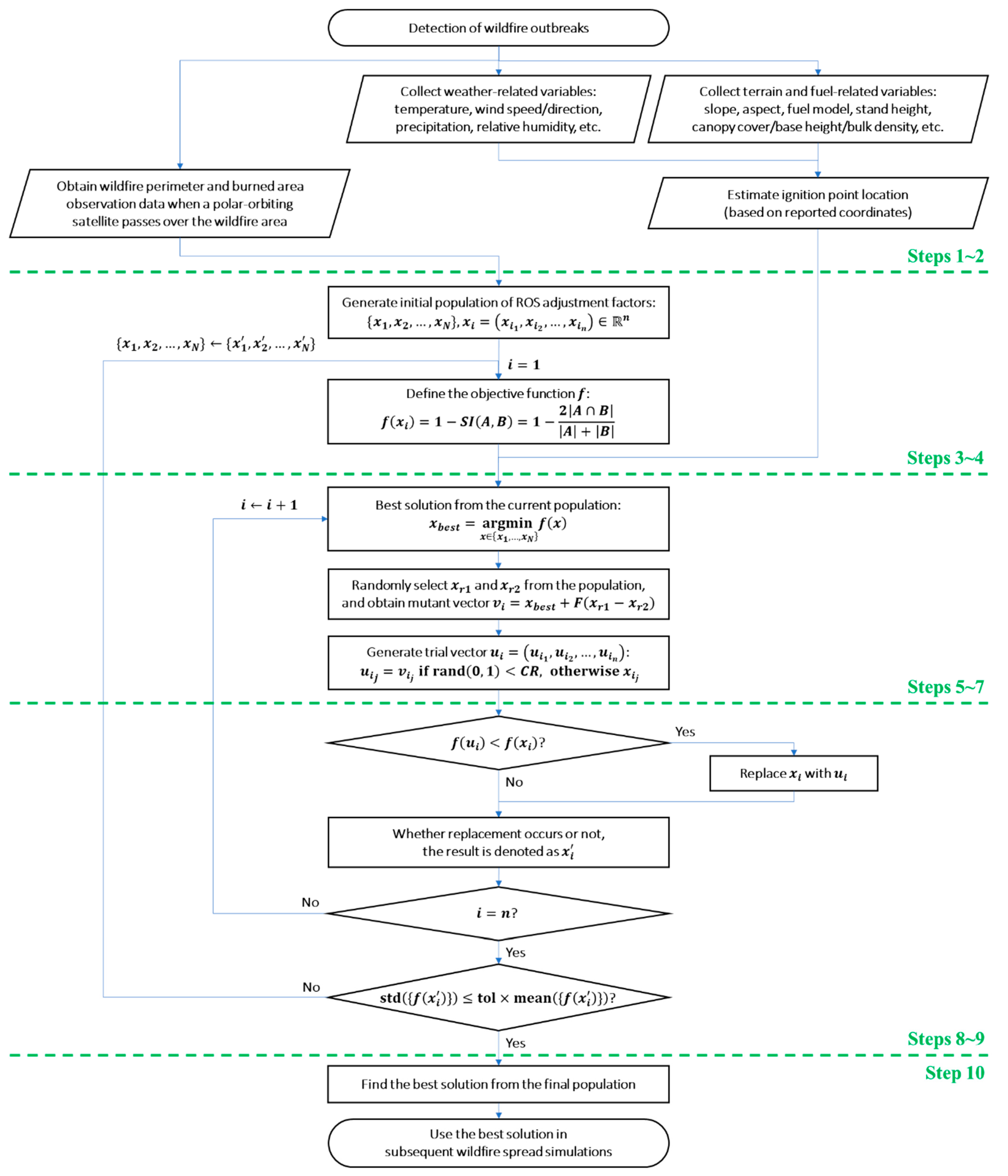
Figure 1. Flowchart of the proposed DE-based algorithm for estimating ROS adjustment factors to reproduce wildfire perimeters observed by polar-orbiting satellites.
Remotesensing 17 02824 g001
Figure 2. Observed wildfire regions (gray regions) and estimated ignition points (green points) at the time of polar-orbiting satellite observation used for methodology validation.
Remotesensing 17 02824 g002
Figure 3. Wildfire prediction results for six wildfire cases; red: prediction result with ROS adjustment factors derived using the proposed methodology, blue: prediction result without ROS adjustment factors, gray: actual wildfire perimeter, and green dot: ignition point. The locations of the gray perimeters and red dots are identical to those shown in Figure 2.
Remotesensing 17 02824 g003
Figure 4. Slope maps within the spread areas of Wildfires #1 and #5 (slope unit: radian), red: observed wildfire perimeters, and green dot: ignition point.
Remotesensing 17 02824 g004
Table 1. Aerial observation data collection tools and their advantages and disadvantages [25].
ToolsAdvantagesDisadvantages
DronesHigher resolution dataVarious constraints
(weather, battery, range, etc.)
Airborne imagingHigher resolution data;
short observation time intervals
Insufficient infrared line scanners:
may not be accessible where wildfire occur
Polar-orbiting satelliteHigh resolution data;
fewer constraints
Longer observation time intervals
Geostationary satelliteShort observation time intervals;
fewer constraints
Lower resolution data
Table 2. List of fuel models defined by Anderson [4].
GroupModel NumberName
Grass1Short Grass
2Timber Grass and Understory
3Tall Grass
Shrub4Chaparral
5Brush
6Dormant Brush
7Southern Rough
Timber8Compact Timber Litter
9Hardwood Litter
10Timber Understory
Slash11Light Slash
12Medium Slash
13Heavy Slash
Table 3. Description of the forest type map data used in this study.
GroupCodeDescription
Age Class *11~10-year-old trees
211~20-year-old trees
321~30-year-old trees
431~40-year-old trees
541~50-year-old trees
6 51-year-old trees
Tree Species10~20Coniferous forest (Korean Pine, Japanese larch, Pitch pine, Black pine, etc.)
30~49Deciduous broadleaf forest (Sawtooth oak, Mongolian oak, East Asian white birch, etc.)
60~68Evergreen broadleaf forest (Bamboo-leaf oak, Camphor tree, etc.)
77Mixed forest
78Bamboo forest
81~82Non-stocked forest land
91~99Non-forest
* Forest stands in which trees of the given age class account for at least 50% of the total canopy cover.
Table 4. Mapping of tree Species to Fuel Models, and Fuel Load, Surface-Area-to-Volume Ratio, and Fuel Depth by Fuel Model Age Class.
Fuel ModelTree SpeciesAge Class CodeFuel Load (kg/m2)SV Ratio (m2/m3)Fuel Depth (m)
0Other Coniferous Trees,
Bamboo
(Bambusoideae)
120.2730.4292000.0260.045
340.6150.3810.0630.087
560.4520.5230.10020.1187
1Korean Red Pine
(Pinus densiflora)
120.2730.4292000.0260.045
340.6150.3810.0630.087
560.4520.5230.10020.1187
2Korean pine
(Pinus koraiensis)
120.440.792000.030.045
340.7510.97130.0450.055
561.12681.18230.06250.07
3Japanese larch
(Larix kaempferi)
120.2570.6782000.0470.054
340.9041.260.0710.08
561.58351.9070.090.1
4Pitch Pine
(Pinus rigida)
120.3210.7642000.030.04
340.7351.02070.050.06
561.22771.43470.070.08
5Black Pine
(Pinus thunbergii)
120.2730.4292000.0260.045
340.6150.3810.0630.087
560.4520.5230.10020.1187
6Other Broadleaf Trees,
Maidenhair Tree
(Ginkgo biloba)
120.3360.4211000.0320.055
340.5150.6030.0590.0757
560.69250.7820.08920.1027
7Oak
(Quercus)
120.3360.4211000.0320.055
340.5150.6030.0590.0757
560.69250.7820.08920.1027
8Mixed forest120.3050.4111500.30.05
340.5240.63230.0550.07
560.74180.85130.08250.095
Table 5. Detailed explanation of the aerial observation data used in the numerical investigation.
Wildfire NumberIgnition TimeSatellite
Observation Time
Observed Wildfire AreaIgnition Point Coordinates (Latitude, Longitude)Fuel Model Types
121 December 2017 21:4721 December 2017 23:503.3049 ha35.89695°N,129.44252°E0, 1, 6, 7
215 January 2021 23:3116 January 2021 01:400.2097 ha36.92391°N,128.50760°E1, 7, 8
310 January 2022 17:3010 January 2022 19:451.0044 ha34.91039°N,127.24240°E0, 1, 4, 6, 8
48 March 2022 20:018 March 2022 22:555.5534 ha35.56734°N,127.56235°E0, 1, 3, 4, 6, 7, 8
512 January 2023 12:4712 January 2023 14:3227.2442 ha35.88449°N,128.13178°E1, 2, 3, 6, 7, 8
63 March 2023 14:023 March 2023 17:562.5238 ha36.49859°N,126.89796°E1, 4, 6, 7, 8
Table 6. Optimized ROS adjustment factors for each wildfire and Sørensen indices with and without the application of the factors. Gray cells indicate fuel models that are not present in the wildfire area.
Wildfire NumberROS Adjustment Factor of Each Fuel ModelSørensen Index
012345678w/ Factorw/o Factor
14.9180.106 3.3661.413 0.7860.366
2 0.106 1.8440.1060.5510.162
30.2200.101 0.112 0.288 1.2170.8960.213
40.6022.204 0.6110.103 1.1080.3862.0420.8210.734
5 1.8692.8622.402 0.1784.9883.6120.4710.145
6 2.516 1.189 0.1050.1011.0100.5910.359
Disclaimer/Publisher’s Note: The statements, opinions and data contained in all publications are solely those of the individual author(s) and contributor(s) and not of MDPI and/or the editor(s). MDPI and/or the editor(s) disclaim responsibility for any injury to people or property resulting from any ideas, methods, instructions or products referred to in the content.