Highlights
What are the main findings?
- A comparison of three widely used tree species mapping approaches using multitemporal Sentinel-2 data revealed no statistically significant differences in classification accuracy;
- The approaches varied significantly in terms of the number of features required for model training and their potential for transferability.
What is the implication of the main finding?
- Multitemporal classification models based on Sentinel-2 imagery can enhance the accuracy of riparian Natura 2000 habitat maps by identifying stands of non-native tree species and mitigating the overestimation of natural habitats;
- Riparian tree species maps can be translated into habitat classifications under the EU Habitats Directive;
- The transferability of tree species classification models to novel geographic regions and temporal contexts must be demonstrated to effectively support large-scale conservation planning, habitat quality assessment, and the evaluation of ecosystem services across Europe.
Abstract
Mapping forest tree species is vital for the habitat assessment, ecosystem services estimation, and implementation of European environmental policies such as the Habitats Directive. This study explores how repeated satellite observations over time, known as multitemporal data, can improve the mapping of tree species in riparian forests. Although many studies have shown that the use of multitemporal data improves tree species classification accuracies, there is a lack of research on how different multitemporal models perform compared to each other. We compared three multitemporal remote sensing approaches using Sentinel-2 imagery to map tree species within the Austrian riparian Natura 2000 site, Salzachauen. Seven tree species (five native and two non-native riparian species) were mapped using random forest models trained on a dataset of 444 validated tree samples. The three multitemporal approaches tested were: (i) multi-date image stacking, (ii) seasonal mean composites, and (iii) spectral–temporal metrics (STMs). The three approaches were compared to twenty single-date image classifications. The multitemporal models achieved 62 to 65% overall accuracy, while the median accuracy of single-date classification was 50% (SD = 6%). The seasonal model obtained the highest overall accuracy (65%), with F1 scores exceeding 73% for four individual species. However, differences among the three multitemporal approaches were not statistically significant. The mapping of native versus non-native riparian species achieved 92% accuracy. We evaluated misclassification patterns of individual species according to the two riparian forest habitats, 91E0* and 91F0, as defined in Annex I of the Habitats Directive. Most omission and commission errors occurred between species within the same habitat type. These findings underline the potential of translating tree species mapping to habitat-type classifications and the need to further explore the capabilities of satellite remote sensing to fill data gaps in Natura 2000 areas.
1. Introduction
Mapping forest tree species composition is crucial for the estimation of ecosystem services, informing policy decisions, and supporting forest management and conservation. Forests are the predominant land cover type in terrestrial protected areas and cover more than 45% of Europe’s total area [1] They provide critical ecosystem services, including habitat provisioning, erosion and flood control, and climate regulation through carbon sequestration [2,3,4,5]. The variety and magnitude of these services are influenced by forests’ tree species composition [6], since individual species vary in structural traits such as wood density, root depth, and water holding capacity [7,8,9,10]. Mapping tree species composition can be translated to maps of forest habitat types [11] as defined in the European Union’s (EU) Habitat Directive [12]. These are essential for monitoring the protected forest areas within the Natura 2000 network and support the implementation of EU’s broader environmental policies such as the Biodiversity Strategy [13], the Forest Strategy [14], the Birds Directive [15] and the Nature Restoration Law [16]. Additionally, tree species maps enable detailed analyses of land cover change, habitat quality [3], and the effects of non-native tree species on ecosystem services [17], serving the needs of forest managers and conservationists.
Traditionally, tree species mapping has relied on labor- and time-intensive fieldwork [18]. This approach is expensive, spatially restricted, and often lacks standardization and external validation, limiting its usefulness in broader environmental monitoring strategies. Remote sensing (RS) images, on the other hand, provide a valuable tool for deriving spatially explicit information on forests, single trees, and tree species composition over large areas at high temporal frequencies. Nowadays, there is a wide variety of RS sensors and platforms used for tree species mapping at different scales [19,20], which are often more cost- and time-efficient compared to lengthy field-based inventories [19].
The two main categories of satellite images used for tree species mapping are very high-resolution (VHR) and high-resolution (HR) images. VHR satellite images with pixel sizes below 1 × 1 m have been used to classify species at the scale of individual tree crowns (ITC) [21,22,23] and can be purchased at price ranges from $3 to $48 per km2 [24]. In contrast to VHR sensors, high-resolution (HR) sensors onboard the Sentinel-2 (S2) satellites provide freely available images with a pixel resolution between 10 m and 20 m and very high temporal resolution (2–5 days). The Landsat satellite missions are another source of freely available HR images; however, they have lower spatial and temporal resolutions [25,26]. Overall, the accessibility of S2 data makes it more suitable than proprietary VHR data for developing standardized mapping methodologies to support European environmental policies [27].
The lower resolution of S2 data means that tree species mapping is conducted at the scale of tree groups/forest stands [11], rather than at the scale of individual tree crowns. The mapping is restricted to the pixel level, as the spectral signal per pixel is used to identify the dominant tree species in the canopy of that pixel [19,28,29]. For such an approach, the broader term “tree species mapping” is used [30,31], where the dominant tree species or, consequently, forest types (e.g., beech forest), are mapped. This contrasts with the term “tree species classification”, which refers to identification at the scale of individual trees.
The classical pixel-based machine learning (ML) classification has been the most used approach for tree species mapping with S2 data, due to the sensor’s coarser resolution and lack of spatial features such as the tree crown texture. Deep learning has also been applied to S2 images to map tree species [29,32], or their proportions, in a single pixel [33]. However, since the training of deep learning models is limited to studies with very large amounts of tree reference data [20,34], classical machine learning methods are still used [28,30,35,36,37,38,39,40,41,42]. While national inventories provide large amounts of forest reference data, these mainly represent the dominant tree species in the European context. In contrast, obtaining comparable amounts of data for less common species, such as those in riparian forests, remains a challenge. Consequently, most studies focus on dominant genera, such as spruce (Picea), larch (Larix), oak (Quercus), beech (Fagus), and fir (Abies), whereas the mapping of forest types defined by less frequent tree species is still limited [30].
The lower spatial and spectral resolutions of S2 data are compensated by their very high temporal resolution, with a 5-day revisit time at the Equator since 2015. Such dense time series enable observations of changes in the vegetation’s seasonal phenological cycles [43], which are distinct among many tree species [44,45]. However, cloud-cover conditions reduce the available image dates for analysis and can significantly influence the recorded phenological patterns [43,46]. Nevertheless, previous studies on tree species mapping have shown that the use of multitemporal images improves overall classification accuracy by up to 5–10% compared to a single-date image classification [28,35,36].
We identified three main approaches using multitemporal data for tree species mapping, which are often considered under the general term ‘time series classification’. These are: (i) combining a selection of multidate images (time series) [28,30,35,36,47]; (ii) using seasonal composites calculated over two to four months [48,49]; and (iii) calculating long-term spectral-temporal variability metrics (STMs) [31,50,51]. Some studies used a combination of multitemporal approaches such as incorporating STMs with time series data [47]. Data cubes are another solution to the multitemporal classification challenge [30]; however, these are rarely used in the field of tree species mapping.
The multidate classification, also referred to as time series classification, is one of the first explored multitemporal approaches for tree species mapping [26,52]. This method combines the band values from each single date in the chosen cloud-free image collection and feeds them to the classifier [28,36]. Usually, the dates are selected to represent different phenological periods [35]. Comparatively, some studies use interpolated time series at equal-day intervals for the whole year [53]. The multi-date approach does not require feature engineering, which makes it straightforward, simple, and intuitive to use. Nevertheless, its high dimensionality can lead to inefficiencies and overfitting in machine learning models, also referred to as the curse of dimensionality [54]. Furthermore, since the feature variables are fully dependent on the dates used, the model cannot be applied to other time periods. Thus, the transferability of the multi-date approach is limited. This can be counteracted with time series interpolation; however, this increases the feature space even more [55].
Seasonal composite approaches utilize the mean or the median pixel values of the chosen season to summarize the time series data for that period [48,49,56]. Composites can focus on critical phenological periods (e.g., peak greenness in summer, senescence in autumn), which are most informative for vegetation classification or monitoring. The limitation of this approach is in defining the seasons to be used and their exact time frames. This requires expert knowledge, as key phenological periods might differ among species. Furthermore, the start of the phenological period can also differ among years due to climatic conditions, which can alter the statistical values of the fixed seasonal time frame. Another challenge is that seasonal boundaries are not universal. They vary across ecosystems, geographic regions, and climate zones. In general, seasonal composites can oversimplify the time series and important temporal variability within the season might be lost.
Instead of defining discrete seasonal periods, STMs aggregate spectral data for the whole year. This omits the need for expert knowledge on the seasonality of different species. However, variations in environmental and climatic conditions still need to be accounted for, especially if the classification is to be applied to larger spatial scales [25,55]. Furthermore, climatic conditions not only influence phenology traits, but also data availability and consistency across regions. Frantz et al. [57] found that there is a significant difference across regions in the multi-annual consistency of Landsat observations and that the temporal distribution of cloud-free images is more important than the number of images, regarding STMs quality.
Although many studies have shown that the use of multitemporal data improves tree species mapping accuracies, there is a lack of research on how different multitemporal models perform compared to each other. This research gap limits our understanding of the advantages and disadvantages associated with different types of multitemporal data. It also reduces the clarity behind researchers’ decisions to choose one multitemporal model over the others. A comparison of multitemporal approaches is needed to discuss their transferability, standardization of the models, and thus advance the use of remote sensing methods for tree species mapping.
This study aims to compare three multi-temporal S2 classification approaches—multi-date stacked image classification, seasonal mean statistics, and STMs—to map five native and two non-native riparian species within a Natura 2000 riparian forest area in Austria. The tree species classification is constrained to the dominant canopy species, detectable at the S2 pixel resolution (10 × 10 m and 20 × 20 m). The multitemporal approaches are further compared to twenty single-date image classifications to test whether multitemporal data improves classification accuracy. Besides evaluating single-species classification accuracies, the binary classification of native versus non-native species groups is assessed. Finally, the potential application of the results for mapping the riparian forest habitats 91E0* and 91F0 under the EU Habitats Directive is discussed. The novelty of this study lies both in the comparison of the multitemporal approaches and in the mapping of less common EU tree species, whose distribution is important for riparian forest conservation.
2. Materials and Methods
2.1. Study Area
The study area is situated in a Natura 2000 riparian site Salzachauen (i.e., AT3209022), Austria (Figure 1). It covers a total of 11.45 km2, out of which forests account for around 6.7 km2. The area is designated as a Special Protected Area (SPA), with some parts also designated as Special Areas of Conservation (SAC). It is located along the Salzach river and represents one of the most biodiverse habitats in the Salzburg province. The included forest habitat types are 91E0* (alluvial forests with Alnus glutinosa and Fraxinus excelsior) and 91F0 (riparian mixed forests of Quercus robur, Ulmus laevis and Ulmus minor, Fraxinus excelsior or Fraxinus angustifolia, along large rivers) as defined in Annex I in the EU Habitats Directive. Native tree species of the area are black alder (Alnus glutinosa), grey alder (Alnus incana), ash (Fraxinus excelsior), oak (Quercus robur), and white willow (Salix alba). The species Alnus incana, Alnus glutinosa and Salix alba are found in habitat 91E0*, whereas Quercus robur is found in 91F0, and Fraxinus excelsior is found in both habitats. Apart from the natural forest habitats, plantations of the non-native species Norway spruce (Picea abies) and balsam poplar (Populus balsamifera) are present.
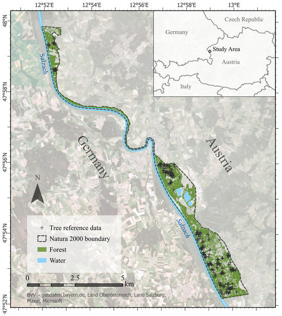
Figure 1.
Area of interest: Salzachauen. Basemap source: Esri Imagery.
2.2. Sentinel-2 Data
Level-2A (surface reflectance) S2 images were queried and used within Google Earth Engine [58], a cloud-computing platform for geospatial analysis. Images covering the area of interest (AOI) were filtered for tile number ‘33UUP’, and the period between 1 January 2018 and 31 December 2020. This period was chosen since no major changes occurred in the riparian forest at that time. To gather sufficient cloud-free images representative of the different seasons, data from multiple years were used. Only the S2-A satellite was used to mitigate bias based on differences between the twin constellation of S2-A and S2-B. Images with any cloud presence were manually excluded from the collection. Ten spectral bands covering the visible, near infrared, and shortwave infrared spectrum were used (Table 1). All bands were resampled to 10 m resolution, and two vegetation indices were calculated for each image (Table 2). The final dataset comprised 20 cloud-free images (Table A1) within the months March to October, consisting of twelve bands each.

Table 1.
Bands and resolution of Sentinel-2 images used in this research.
Table 2.
Indices used in this study as additional bands to each image.
Vegetation indices have high feature importance in tree species classification and increase classification accuracies [30,36,55]. The normalized difference vegetation index (NDVI), according to Tucker [59], and the Greenness index according to Baraldi et al. [60], were used (Table 2). The former index is more spectrally sensitive to red reflectance, while the latter is more sensitive to the near and mid infrared reflectance [60]. The combination of such two indices allows for a better characterization of the forest cover in contrast to NDVI only [61].
2.3. Tree Reference Data and Pre-Processing
A total of 653 tree coordinate points representing individual trees were available from previous in-field studies. The data (Figure 1) were obtained in the years 2012 (28 points), 2022 (425 points), and 2023 (200 points). Single tree locations were collected in the field with the support of an orthophoto, LiDAR-nDSM maps, and DGNSS for in-field orientation. This dataset was increased with 308 points derived through visual interpretation of a 2020 orthophoto (20 cm spatial resolution) and a 2016 normalized digital surface model (nDSM), supported by the authors’ expert knowledge of the region. The final reference dataset contains 961 coordinate points for 33 tree species. Since the collection of field points was not conducted in the same years as S2 image acquisitions, a visual evaluation based on the 2020 orthophoto was conducted. This ensured that each of the tree points was still present for the period analyzed for this study.
To adapt the reference data for S2 image classification, preprocessing was carried out in ArcGIS Pro. Only those reference points situated within the 10 × 10 m S2 pixel dominated by a single tree species, as apparent in the uppermost canopy level (pure pixel), were used (Figure 2). The mixed/pure pixels situation of the forest stands was verified using orthophoto images from 2020 and LiDAR data from 2016, in combination with field notes of reference data, pointing out whether the recorded tree was single-standing or within a homogenous forest stand. Doubling-points in a single 10 m pixel were removed. Species with less than 50 points of reference data left after the preprocessing were not considered. This resulted in a final reference dataset of 444 points and seven tree species (Table 3), in contrast to the 961 points and 33 tree species initially available. The seven tree species of the final dataset were the most representative of the area, as well as for the riparian forest habitats 91E0* and 91F0, according to the Habitats Directive [12], which were the interest of this study. The excluded species were rare and non-common riparian species, represented only in a few individual trees, or found in the understory of the forest.
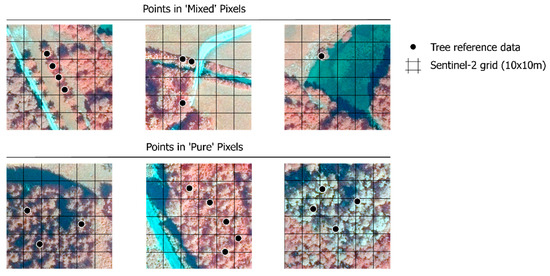
Figure 2.
Example of reference points of trees considered to be in ‘mixed’ or ‘pure’ pixel situations, evaluated against the Sentinel-2 grid (10 × 10 m, tile 33UUP) and a 0.2 m resolution orthophoto (© SAGIS, 2020. Band combination: near-infrared, green, blue).
Table 3.
The number of samples of different tree species. The acronyms of the species are obtained from the first two letters in each Latin name.
For the 20 × 20 m resolution pixels, both pure and mixed situations were considered, with this information recorded in an additional attribute of the reference data points. Reference data of the different species had different amounts of mixed pixels in the 20 m bands (Table 3). This information enabled us to test the impact of the 20 m spectral bands on classification results and to reduce bias in the accuracy assessment that could result from using only pure forest stands [30].
The reference points of each species were randomly split into a 70/30 ratio for training and testing, respectively, using the tool Subset Features (Geostatistical Analyst) in ArcGIS Pro. All random forest ML models were trained and tested on the same set of training and testing data. The pure and mixed pixels (20 × 20 m) of each species were split separately into a 70/30 ratio. This ensured that the training and the testing data had an equal ratio of mixed and pure pixels in the 20 m band. The minimum distance criteria between training and testing points were set to 20 m to mitigate the effects of spatial autocorrelation. The full technical workflow is described in Figure 3.
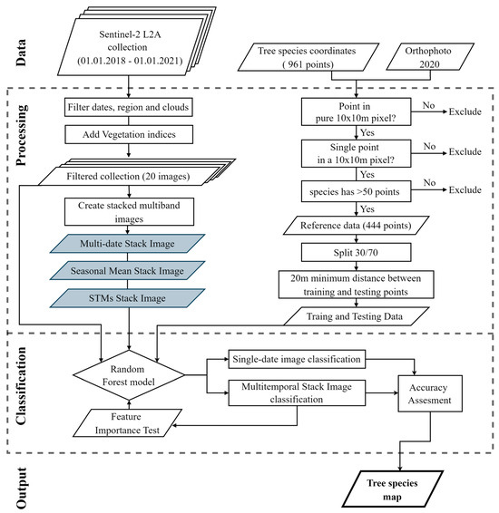
Figure 3.
Technical route map.
2.4. Methodology
In addition to the single-date image collection, we explored three multitemporal approaches: (i) combining all available single-date images in one multi-date stacked image; (ii) combining seasonal mean composites; and (iii) calculation of spectral-temporal metrics (STMs). A multiband stacked image was created for each approach.
The multidate classification is applied by creating a single multitemporal stacked image, containing all spectral bands from each date in the time series. For a time series with n dates and b spectral bands per date, the final image would have n × b bands. In this study, 20 multi-date images were used (Table A1), with 12 bands each, to create a 240-band stacked image.
The inter-seasonal stacked image in this study was created out of three mean composite images: for spring (19 April–18 May); summer (3 June–27 June); and autumn (5 September–15 September). These timeframes were chosen based on the spectral reflectance time series of the tree species in the training dataset and is in accordance with Grabska et al. [28]. The result is a 36-band image composed of 3 seasonal images, each containing 12 bands representing the mean band values of the corresponding season.
STMs were calculated for the entire period (1 January 2018–1 January 2021) and included statistical values for mean, median, standard deviation, variance, first quartile (25th percentile), and the third quartile (75th percentile) for each band. Minimum and maximum values were not included as they are more likely to be influenced by outliers. The resulting STMs stacked image thus included 72 bands.
In total, 23 random forest machine learning classifiers, according to Breiman [62], were trained and applied in GEE using 150 decision trees and an 0.9 bag of fraction. The RF algorithm is one of the most widely used ML algorithms for remote sensing classification [63] as well as for S2 tree species mapping [28,30,35,36,37,38,39,40,41,42], since it is robust to noise, is suitable for high-dimensional data, and is, by design, a multi-class classifier [63]. Twenty separate models were trained for each single-image date, while three models were trained on the multitemporal stacked images. The model that achieved the highest F1 score was used to map areas of non-native and native riparian tree species. Areas classified as non-native were then overlaid with, and compared to, an official Natura 2000 map of alluvial and riparian mixed forest obtained in 2020.
To keep the process simple, the focus was set solely on tree species classification; general forest and non-forest classification was not performed in advance. For better visualization of the results, non-forest areas were masked out using a 5 m tree-height threshold of LiDAR data from 2023. In addition, a Pleiades image acquired on 30 July 2020 (50 cm resolution) was used solely as visual input to the final map displays.
The relative feature importance was calculated by normalizing the absolute values of the “importance” attribute, returned by GEE when running a random forest (RF) model. GEE’s implementation of random forest is based on the SMILE (Statistical Machine Intelligence and Learning Engine) library, where feature importance is provided as the sum of the decrease in the Gini impurity index over all trees in the forest [64].
Accuracy assessment was conducted using precision (user’s accuracy) (Equation (1)); recall (producer’s accuracy) (Equation (2)); overall accuracy (Equation (3)); and F1 scores (Equation (4)); these were obtained from the confusion matrix of each classification approach:
where TP is true positives, TN is true negatives, FP is false positives, and FN is false negatives.
For the statistical comparison of classification, McNemar’s [65] chi-squared () test was applied as a common non-parametric test. It is used to compare the ability of two models to detect the presence or absence of a class. It tests for a significant difference between the models, whereas the null hypothesis is that there is no difference. The McNemar [65] test calculates the instances for each class, where both models are correct, both models are wrong and when one model is correct while the other is wrong. For this purpose, a 2 × 2 contingency table is created for each class, where accuracy metrics (TP, TN, FP, FN) are reduced to a binary classification representing one class versus the rest.
In medical studies, McNemar’s test is most often applied to both sensitivity (precision) and specificity metrics corresponding to the model’s ability to detect the presence or absence of a class, respectively [66]. In medical research, detecting the absence of a disease in some cases might be as important as detecting its presence; however, in landcover classification, the focus is usually on detecting only the presence of a certain landcover. Similarly to previous studies in land cover classification [67,68,69], this study performs McNemar’s test only based on landcover presence (sensitivity).
The McNemar test is a pair-wise test, which means that it can compare only two classifiers at once. In our case, with three classifiers in total, we performed the test on three classification pairs: Multi-date v. Seasonal, Multi-date v. STMs, and STMs v. Seasonal, using Equation (5), as follows:
where is the sum of instances when classification one is correct and classification two is incorrect, and is the sum of instances when classification two is correct while classification one is wrong.
3. Results
3.1. Accuracy Assessment
The overall accuracy of single-date classification ranged between 37% to 58%, with a median accuracy across all dates of 50% (Table 4). The multitemporal approaches, on the other hand, obtained between 62% and 65% overall accuracy. The seasonal composite classification, outlined in Figure 4 and Figure 5, showed the highest results compared to STMs and the multi-date stacked image (Table 4 and Table 5). With this approach, four out of seven species had an F1 score above 73%, while no single-date image reached that accuracy for more than two species. Based on the class-wise McNemar’s tests, no significant difference between the seasonal composites’ classification and the other two multitemporal approaches was found for those species (Table 6). Three single-date classifications (on 19 April 2018, 8 May 2020, and 27 June 2020) with an overall accuracy of 57–58% did not show class-wise statistical difference to any of the multitemporal models. The rest of the single-date classification had a significantly lower accuracy at the 10% level (p ≤ 0.10) for at least one tree species class.
Table 4.
Tree species accuracy assessment of each single-date image classification and of multitemporal stack images.
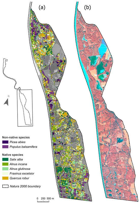
Figure 4.
Tree species classification map of the inter-seasonal stacked image (a), compared to a VHR resolution Pleiades image (b) (July 2020. Band combination: near-infrared, green, red).
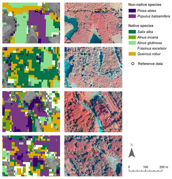
Figure 5.
Classification results of inter-seasonal stacked image on the left compared to orthophotos on the right (© SAGIS, 2020. Band combination: near-infrared, green, blue). Tree species validation points are illustrated as black circles, filled with the corresponding class color of tree species.
Table 5.
Class-wise accuracy metrics for each multitemporal classification type.
Table 6.
McNemar’s test p-values on classification recall (producer’s accuracy).
The species Picea abies, Populus balsamifera, Alnus incana, and Salix alba reached F1 accuracies above 70% throughout the multitemporal and the single-date classifications. The rest of the species, Fraxinus excelsior, Quercus robur, and Alnus glutinosa, showed similar spectral patterns in time with resulting accuracies between 30% and 53% in the multitemporal models (Figure 6). Accuracy for those species in the single-date models ranged between 7% and 52%. When comparing Greenness to NDVI time series, the former showed a slightly better separability of species and improved data exploration (Figure 6 and Figure 7). The same was true for value distributions of the two bands (Figure A1 and Figure A2).
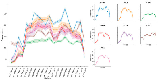
Figure 6.
Time series of the Greenness index across tree species. The dates format is provided as mm/dd/yyyy.
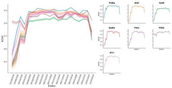
Figure 7.
Time series of the NDVI index across tree species. The dates format is provided as mm/dd/yyyy.
3.2. Feature Importance
The NDVI and the Greenness bands had the highest feature importance score in the multi-date stacked image (Figure 8). They were among the most important bands for STMs as well, in addition to B11 and B12 (Figure A3). For the inter-seasonal image, the importance of NDVI and B5 bands were predominant (Figure A4). From a temporal perspective, the multidate classification approach identified April, June, and July as the most significant months (Figure 8). In the single-date classification, single species reached their highest classification accuracies also in April and June, as well as in the first half of May (Table 4). All seasonal composites were important for the classification; no distinct pattern was observed there. For the STMs, there was a clear dominance of the standard deviation and variance metrics in terms of importance, especially for B11, B12, Greenness, and NDVI (Figure A3). Populus balsamifera and Alnus incana were the species that benefited the most from the multitemporal approach. In the single-date classification, the maximum accuracy achieved for the two species was 72% and 71%, respectively. In comparison, their accuracy in the multitemporal images reached 83% and 76%.
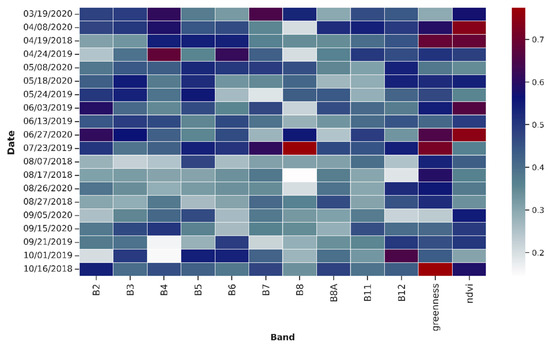
Figure 8.
Relative feature importance of multi-date classification. The dates format is provided as mm/dd/yyyy.
3.3. Impact of Mixed Pixels in the 20 M Bands
Visual interpretation of the inter-seasonal tree species classification map revealed satisfactory results in homogeneous forest stands (Figure 5). Nevertheless, the evaluation of mixed pixels revealed a strong correlation between species classification accuracy and the number of reference points of each species located within mixed 20 × 20 m pixels (Figure 9). There was a higher correlation in the mixed pixels of testing samples rather than in the training data. A high correlation was also shown between the overall number of reference points and classification accuracy.
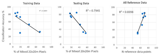
Figure 9.
Comparison of tree species classification accuracy with percentage of training points in mixed pixels (20 × 20 m), percentage of testing points in mixed pixels, and the total number of reference points.
3.4. Autochthonous Versus Allochthonous Tree Species and Habitat-Level Patterns
Even though findings on the level of single species did not show high accuracies, the model achieved 92% accuracy in classifying native (autochthonous) versus non-native (allochthonous) riparian species (Figure 10). We found 17.4 hectares of overlap between Natura 2000 riparian habitats (91E0* and 91F0) and areas of non-native tree species (Figure 11). A visual comparison of the results with orthophoto image of 2020 confirmed the presence of non-native forest stands in the Natura 2000 area.
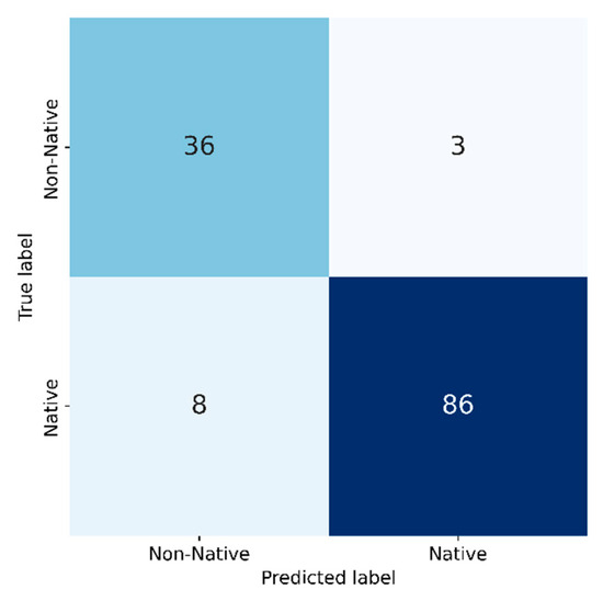
Figure 10.
Confusion matrix based on whether tree species are native to riparian forests according to the Habitats Directive.
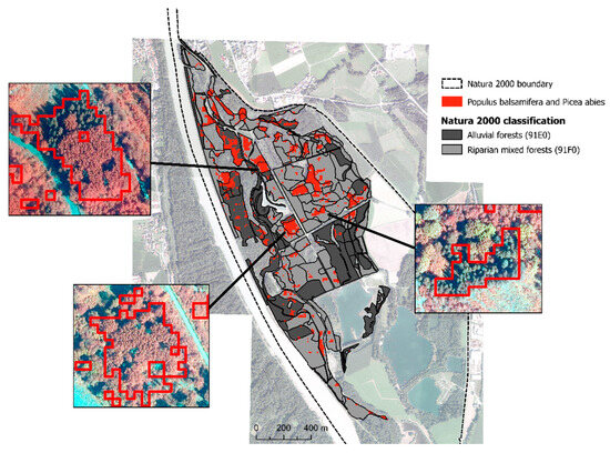
Figure 11.
Classification of non-native tree species Populus balsamifera and Picea abies, which intersect with Natura 2000 riparian forest habitats (91E0* and 91F0). Orthophotos are included for reference (© SAGIS, 2020. Band combination: near-infrared, green, blue).
Evaluation of the confusion matrix of our best classification model showed that single species are most often under/overestimated with species of the same habitat class (Figure 12). This is not true only for Fraxinus excelsior, since it was found in both classes. For example, Salix alba achieved 67% user accuracy. However, the species was overestimated, with Alnus glutinosa, Alnus incana and Fraxinus excelsior representing the same habitat type. The producer’s accuracy of Alnus incana was 64%; however, 32% of the omitted reference points belonged again to species of the same habitat class.
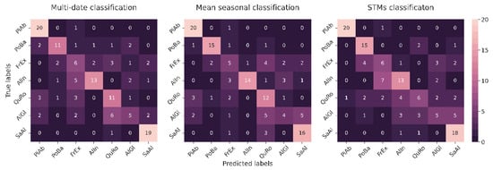
Figure 12.
Error matrices show the results of each multitemporal classification approach.
4. Discussion
Similar to previous studies [28,30,35,36,37,38,39,40,41,42], the current research confirms that the use of multitemporal data improves RF classification models for tree species mapping. In addition, we compared three multitemporal approaches within a small, protected riparian forest. The results showed no significant difference in the accuracy between the three approaches. However, these findings are limited to the species investigated in this study and to the RF method. Future research should consider the growing potential of deep learning for tree species mapping [20]. A focus should also be placed on improving our understanding of different multitemporal approaches across multiple spatial scales and tree species.
The three multitemporal approaches compared in this study did not differ significantly in accuracy; however, they varied substantially in terms of transferability and computational requirements. For example, the multi-date classification used six times more features (240 bands) than the seasonal classification (36 bands) and three times more features than the STMs classification (72 bands). In contrast to the multi-date classification, seasonal and STMs classification use aggregated band values over time. These approaches have the advantage of noise reduction, decreased feature space, and lower data storage and processing. Nevertheless, the robustness of those approaches under varying cloud-free image availability [43] needs to be further researched to better assess their transferability. While the transferability of ML models for tree species mapping is rarely addressed, it is crucial for enabling RS applications to support monitoring for EU environmental policies.
Studies focusing on common European tree species have reported overall accuracies above 80% [30,48,55], while this study achieved a maximum overall classification accuracy of 65%. However, the results of previous studies vary with species; the classification of less common species remains challenging. In the current study, only spruce (Picea abies) and oak (Quercus robur) can be considered as common European species, while the five other species are part of the less common genera Populus (poplar), Fraxinus (ash), Alnus (alder), and Salix (willow).
The F1 classification accuracies for Salix alba, Populus balsamifera, and Alnus incana exceeded values reported in previous work [28,30,55]. By contrast, the classification accuracy of Quercus robur—a common European species—was lower than that of the stated studies. This is likely because those studies used oak-dominated forest stands as reference, while in this study, only data for single-planted oak trees dominant in 10 × 10 m pixels were available. Alnus glutinosa showed an accuracy of only 30–36%, potentially due to the quality of the reference data and the absence of topographic predictors commonly used elsewhere [28,30]. Fraxinus excelsior also had low accuracy (<39%), consistent with other studies, as it typically occurs as scattered individuals in mixed stands [30,70]. Overall, direct comparison to previous studies is not straightforward, as these classified a greater number of species over larger areas. Future work should extend to less common European species, especially those of ecological relevance and linked to Habitat Directive habitat types [71].
The evaluation of the mixed-pixels situation showed a high correlation between the classification accuracy and the amount of mixed pixels in the reference data of the 20 m bands. Tree species that contained a higher number of pure 20 m pixels achieved higher accuracies. These findings are important because previous studies claimed a classification map resolution of 10 m. However, they used only pure 20 m pixels for validation. Such a classification approach simplifies the forest landscape and introduces a bias towards higher classification accuracies. Similar to Blickensdörfer et al. [30], this research suggests that the accuracy assessment of future studies should be more representative, including pure and mixed pixels, both in the centers and edges of forest polygons. Nevertheless, we acknowledge that the present study relies on a limited amount of reference data for evaluating the correlation; future research should use larger datasets to strengthen the validity of this statement.
Results from the feature importance test confirmed the importance of vegetation index bands in tree species classification [36,55]. The vegetation indices from the early growing season (April, May) were most important for tree species classification, consistent with that of Hemmerling et al. [55] and Grabska et al. [28,48]. While previous studies underline the importance of the NDVI index [30,72] our results demonstrate better separability of tree species with the use of the Greenness index [60]. Disadvantages of the commonly used NDVI index have been described by Baraldi et al. [60]; these include the influence of the background signal in cases of a low leaf area index (LAI); saturation of the NDVI values if the canopy is too dense; and a non-linear relationship between the LAI and the NDVI. More applied research is needed, however, to further strengthen these assumptions, particularly for the purpose of tree species mapping.
Despite lower accuracies for some single species, the seasonal model achieved 92% accuracy in classifying native versus non-native riparian species. The introduced riparian species, Populus balsamifera and Picea abies, were mostly found in pure forest stands, with strong spectral signatures, which is likely the reason for their higher classification accuracies. While this is not surprising from an RS methodological point of view, this observation has practical implications for updating Natura 2000 maps. For instance, we found an 8% overlap between non-native species areas and the official Natura 2000 riparian forest map of the Salzachauen (Figure 11). This approach has high potential for improving existing Natura 2000 maps and reducing overestimation of natural habitat areas. Maps of native versus non-native tree species can also be a valuable input to habitat quality evaluation [3,73] and ecosystem services estimation [17].
Further implementation of the three species maps produced in this study would be their translation into the corresponding Annex I habitat type of the EU Habitats Directive [11]. Our results showed that misclassification of single native species occurs with species of the same habitat class (91E0* and 91F0). This demonstrates the potential of tree species mapping for habitat type classification in order to fill data gaps in Natura 2000 areas [71]. A relevant question for future research is whether tree species of the same habitat type have similar phenology, which can potentially improve the separation and mapping of those habitats. Unfortunately, the present study lacked enough reference data to test this hypothesis. Future work should therefore focus on identifying the phenological spectral curves of tree species (through field spectroradiometer observations or temporal gap-filling of satellite-derived time series data) to evaluate whether incorporating phenological patterns can improve habitat classification.
5. Conclusions and Outlook
This study underlines the potential of using multitemporal Sentinel-2 imagery for the classification of tree species within riparian forests, with particular attention to distinguishing between native and non-native species. The RF models based on the multitemporal approach demonstrated a significantly higher overall classification accuracy compared to models based on single-date analyses. The seasonal multitemporal approach achieved above 73% accuracy for four individual species and 92% overall accuracy for classifying native versus non-native species. Nonetheless, these results apply specifically to machine learning classification using RF; further research is required to extend them to the rapidly growing field of deep learning for tree species mapping.
The findings highlight the importance of vegetation indices, especially those obtained during the early growing season (April and May), for effective tree species classification. However, the study also revealed challenges related to mixed pixels at 20 × 20 m resolution, which influenced classification accuracy. Species with a higher ratio of pure pixels achieved better classification results, suggesting that future studies should consider both pure and mixed pixels in accuracy assessments to avoid bias and ensure a more comprehensive representation of the forest landscape.
The successful identification of non-native species within a Natura 2000 protected area emphasizes the practical applications of this methodology for environmental monitoring and management. By providing maps of native and non-native species distribution, this approach can support spatial planning for the habitat restoration of riparian forests and inform policy decisions, particularly those related to the EU Habitats Directive, by providing additional information on habitat distribution and conditions. To achieve this, more research focused on less common, but ecologically significant, tree species is needed, accompanied by a higher quantity and quality of reference data. Future work should also explore, in more detail, the scope of spectral–temporal metrics for improving classification accuracy and transferability. Finally, translating such tree species classification models into habitat type maps should be practically evaluated for the management and monitoring needs of data-poor Natura 2000 areas.
Author Contributions
Conceptualization, Y.R., H.K. and T.S.; data curation, Y.R.; formal analysis, Y.R.; funding acquisition, H.K. and T.S.; investigation, Y.R.; methodology, Y.R.; project administration, Y.R., H.K. and T.S.; resources, Y.R. and T.S.; supervision, H.K. and T.S.; validation, H.K. and T.S.; visualization, Y.R.; writing original draft and review, Y.R.; writing review, H.K. and T.S. All authors have read and agreed to the published version of the manuscript.
Funding
We acknowledge support and funding from the project Science for Evidence-based and Sustainable Decisions about Natural Capital (SELINA, grant agreement No. 101060415) funded by the European Union’s Horizon Europe research and innovation program. This work was also supported through the project EOai4BIO funded by the Austrian Research Promotion Agency under the Austrian Space Applications Programme (ASAP 18, contract no.: 892669).
Data Availability Statement
The tree species data and the Google Earth Engine code used in this study are freely available at the following GitHub (git version 2.34.1) repository: https://github.com/nikolovayana/Sen2Tree_multitemporal (accessed on 10 September 2025). Orthophotos and LiDAR data were kindly provided by the Administration of the federal state of Salzburg.
Acknowledgments
Special acknowledgement is also made to the current and past managers of the Natura 2000 site Salzachauen (i.e., AT3209022) for providing access to the area and sharing additional data for its habitat classification. We would also like to thank the. Open Access Funding provided by the University of Salzburg.
Conflicts of Interest
The authors declare no conflicts of interest. The funders had no role in the design of the study; in the collection, analyses, or interpretation of data; in the writing of the manuscript; or in the decision to publish the results.
Appendix A
Table A1.
Cloud-free image collection obtained in Google Earth Engine.
Table A1.
Cloud-free image collection obtained in Google Earth Engine.
| Date | Day of the Year | Image ID |
|---|---|---|
| 19 March 2020 | 79 | COPERNICUS/S2_SR_HARMONIZED/20200319T101021_20200319T101336_T33UUP |
| 8 April 2020 | 99 | COPERNICUS/S2_SR_HARMONIZED/20200408T101021_20200408T101022_T33UUP |
| 19 April 2018 | 109 | COPERNICUS/S2_SR_HARMONIZED/20180419T101031_20180419T101457_T33UUP |
| 24 April 2019 | 114 | COPERNICUS/S2_SR_HARMONIZED/20190424T101031_20190424T101032_T33UUP |
| 8 May 2020 | 129 | COPERNICUS/S2_SR_HARMONIZED/20200508T101031_20200508T101648_T33UUP |
| 18 May 2020 | 139 | COPERNICUS/S2_SR_HARMONIZED/20200518T101031_20200518T101258_T33UUP |
| 24 May 2019 | 144 | COPERNICUS/S2_SR_HARMONIZED/20190524T101031_20190524T101701_T33UUP |
| 3 June 2019 | 154 | COPERNICUS/S2_SR_HARMONIZED/20190603T101031_20190603T101642_T33UUP |
| 13 June 2019 | 164 | COPERNICUS/S2_SR_HARMONIZED/20190613T101031_20190613T101027_T33UUP |
| 27 June 2020 | 179 | COPERNICUS/S2_SR_HARMONIZED/20200627T101031_20200627T101243_T33UUP |
| 23 July 2019 | 204 | COPERNICUS/S2_SR_HARMONIZED/20190723T101031_20190723T101347_T33UUP |
| 7 August 2018 | 219 | COPERNICUS/S2_SR_HARMONIZED/20180807T101021_20180807T101024_T33UUP |
| 17 August 2018 | 229 | COPERNICUS/S2_SR_HARMONIZED/20180817T101021_20180817T101024_T33UUP |
| 26 August 2020 | 239 | COPERNICUS/S2_SR_HARMONIZED/20200826T101031_20200826T101345_T33UUP |
| 27 August 2018 | 239 | COPERNICUS/S2_SR_HARMONIZED/20180827T101021_20180827T101023_T33UUP |
| 5 September 2020 | 249 | COPERNICUS/S2_SR_HARMONIZED/20200905T101031_20200905T101637_T33UUP |
| 15 September 2020 | 259 | COPERNICUS/S2_SR_HARMONIZED/20200915T101031_20200915T101550_T33UUP |
| 21 September 2019 | 264 | COPERNICUS/S2_SR_HARMONIZED/20190921T101031_20190921T101152_T33UUP |
| 1 October 2019 | 274 | COPERNICUS/S2_SR_HARMONIZED/20191001T101031_20191001T101659_T33UUP |
| 16 October 2018 | 289 | COPERNICUS/S2_SR_HARMONIZED/20181016T101021_20181016T101021_T33UUP |

Figure A1.
Distribution of Greenness values recorded for the time-period 2018–2020 for each tree species.

Figure A2.
Distribution of NDVI values recorded for the time-period 2018–2020 for each tree species.

Figure A3.
Feature importance test on STMs stack image.

Figure A4.
Feature importance test on inter-seasonal stack image consisting of mean seasonal composites.
References
- UNSDG. Available online: https://unstats.un.org/sdgs/dataportal (accessed on 28 March 2024).
- Brockerhoff, E.G.; Barbaro, L.; Castagneyrol, B.; Forrester, D.I.; Gardiner, B.; González-Olabarria, J.R.; Lyver, P.O.; Meurisse, N.; Oxbrough, A.; Taki, H.; et al. Forest Biodiversity, Ecosystem Functioning and the Provision of Ecosystem Services. Biodivers. Conserv. 2017, 26, 3005–3035. [Google Scholar] [CrossRef]
- Riedler, B.; Lang, S. A Spatially Explicit Patch Model of Habitat Quality, Integrating Spatio-Structural Indicators. Ecol. Indic. 2018, 94, 128–141. [Google Scholar] [CrossRef]
- Sutherland, I.J.; Gergel, S.E.; Bennett, E.M. Seeing the Forest for Its Multiple Ecosystem Services: Indicators for Cultural Services in Heterogeneous Forests. Ecol. Indic. 2016, 71, 123–133. [Google Scholar] [CrossRef]
- Vorster, A.G.; Evangelista, P.H.; Stovall, A.E.L.; Ex, S. Variability and Uncertainty in Forest Biomass Estimates from the Tree to Landscape Scale: The Role of Allometric Equations. Carbon Balance Manag. 2020, 15, 8. [Google Scholar] [CrossRef] [PubMed]
- Gamfeldt, L.; Snäll, T.; Bagchi, R.; Jonsson, M.; Gustafsson, L.; Kjellander, P.; Ruiz-Jaen, M.C.; Fröberg, M.; Stendahl, J.; Philipson, C.D.; et al. Higher Levels of Multiple Ecosystem Services Are Found in Forests with More Tree Species. Nat. Commun. 2013, 4, 1340. [Google Scholar] [CrossRef] [PubMed]
- Bouchard, E.; Searle, E.B.; Drapeau, P.; Liang, J.; Gamarra, J.G.P.; Abegg, M.; Alberti, G.; Zambrano, A.A.; Alvarez-Davila, E.; Alves, L.F.; et al. Global Patterns and Environmental Drivers of Forest Functional Composition. Glob. Ecol. Biogeogr. 2024, 33, 303–324. [Google Scholar] [CrossRef]
- Comas, L.; Bouma, T.; Eissenstat, D. Linking Root Traits to Potential Growth Rate in Six Temperate Tree Species. Oecologia 2002, 132, 34–43. [Google Scholar] [CrossRef]
- Mitchell, R.J.; Hewison, R.L.; Haghi, R.K.; Robertson, A.H.J.; Main, A.M.; Owen, I.J. Functional and Ecosystem Service Differences between Tree Species: Implications for Tree Species Replacement. Trees 2021, 35, 307–317. [Google Scholar] [CrossRef]
- Mo, L.; Crowther, T.W.; Maynard, D.S.; van den Hoogen, J.; Ma, H.; Bialic-Murphy, L.; Liang, J.; de-Miguel, S.; Nabuurs, G.-J.; Reich, P.B.; et al. The Global Distribution and Drivers of Wood Density and Their Impact on Forest Carbon Stocks. Nat. Ecol. Evol. 2024, 8, 2195–2212. [Google Scholar] [CrossRef]
- Strasser, T.; Lang, S. Object-Based Class Modelling for Multi-Scale Riparian Forest Habitat Mapping. Int. J. Appl. Earth Obs. Geoinf. 2015, 37, 29–37. [Google Scholar] [CrossRef]
- Official Journal of the European Union. Council Directive 92/43/EEC of 21 May 1992 on the Conservation of Natural Habitats and of Wild Fauna and Flora; L 206. 22 July 1992, pp. 7–50. Available online: https://eur-lex.europa.eu/legal-content/EN/TXT/?uri=CELEX%3A31992L0043 (accessed on 10 September 2025).
- European Commission. Communication from the Commission to the European Parliament, The Council, The European Economic and Social Committee and the Committee of the Regions EU Biodiversity Strategy for 2030 Bringing Nature Back into Our Lives; COM/2020/380 Final; Publications Office of the European Union: Brussels, Belgium, 2020; Available online: https://eur-lex.europa.eu/legal-content/EN/TXT/?uri=CELEX:52020DC0380 (accessed on 10 September 2025).
- European Commission. Communication from the Commission to the European Parliament, The Council, The European Economic and Social Committee and the Committee of the Regions New EU Forest Strategy for 2030; COM/2021/572 Final; Publications Office of the European Union: Brussels, Belgium, 2021; Available online: https://eur-lex.europa.eu/legal-content/EN/TXT/?uri=celex:52021DC0572 (accessed on 10 September 2025).
- Official Journal of the European Union. European Parliament Directive 2009/147/EC of the European Parliament and of the Council of 30 November 2009 on the Conservation of Wild Birds (Codified Version); L20/7. 2009. Available online: https://eur-lex.europa.eu/legal-content/EN/TXT/?uri=CELEX:32009L0147 (accessed on 10 September 2025).
- Official Journal of the European Union. European Parliament Regulation (EU) 2024/1991 of the European Parliament and of the Council of 24 June 2024 on Nature Restoration and Amending Regulation (EU) 2022/869 (Text with EEA Relevance). 2024. Available online: https://eur-lex.europa.eu/eli/reg/2024/1991/oj/eng (accessed on 10 September 2025).
- Castro-Díez, P.; Vaz, A.S.; Silva, J.S.; van Loo, M.; Alonso, Á.; Aponte, C.; Bayón, Á.; Bellingham, P.J.; Chiuffo, M.C.; DiManno, N.; et al. Global Effects of Non-Native Tree Species on Multiple Ecosystem Services. Biol. Rev. 2019, 94, 1477–1501. [Google Scholar] [CrossRef] [PubMed]
- McRoberts, R.E.; Tomppo, E.O.; Næsset, E. Advances and Emerging Issues in National Forest Inventories. Scand. J. For. Res. 2010, 25, 368–381. [Google Scholar] [CrossRef]
- Fassnacht, F.E.; Latifi, H.; Stereńczak, K.; Modzelewska, A.; Lefsky, M.; Waser, L.T.; Straub, C.; Ghosh, A. Review of Studies on Tree Species Classification from Remotely Sensed Data. Remote Sens. Environ. 2016, 186, 64–87. [Google Scholar] [CrossRef]
- Zhong, L.; Dai, Z.; Fang, P.; Cao, Y.; Wang, L. A Review: Tree Species Classification Based on Remote Sensing Data and Classic Deep Learning-Based Methods. Forests 2024, 15, 852. [Google Scholar] [CrossRef]
- Fassnacht, F.E.; Neumann, C.; Förster, M.; Buddenbaum, H.; Ghosh, A.; Clasen, A.; Joshi, P.K.; Koch, B. Comparison of Feature Reduction Algorithms for Classifying Tree Species With Hyperspectral Data on Three Central European Test Sites. IEEE J. Sel. Top. Appl. Earth Obs. Remote Sens. 2014, 7, 2547–2561. [Google Scholar] [CrossRef]
- Ghosh, A.; Fassnacht, F.E.; Joshi, P.K.; Koch, B. A Framework for Mapping Tree Species Combining Hyperspectral and LiDAR Data: Role of Selected Classifiers and Sensor across Three Spatial Scales. Int. J. Appl. Earth Obs. Geoinf. 2014, 26, 49–63. [Google Scholar] [CrossRef]
- Pu, R.; Liu, D. Segmented Canonical Discriminant Analysis of in Situ Hyperspectral Data for Identifying 13 Urban Tree Species. Int. J. Remote Sens. 2011, 32, 2207–2226. [Google Scholar] [CrossRef]
- LandInfo—Imagery Pricing. Available online: https://landinfo.com/satellite-imagery-pricing/ (accessed on 10 September 2025).
- Hermosilla, T.; Bastyr, A.; Coops, N.C.; White, J.C.; Wulder, M.A. Mapping the Presence and Distribution of Tree Species in Canada’s Forested Ecosystems. Remote Sens. Environ. 2022, 282, 113276. [Google Scholar] [CrossRef]
- Wolter, P.; Mladenoff, D.; Host, G.; Crow, T. Improved Forest Classification in the Northern Lake States Using Multi-Temporal Landsat Imagery. Photogramm. Eng. Remote Sens. 1995, 61, 1129. [Google Scholar]
- Vanden Borre, J.; Paelinckx, D.; Mücher, C.A.; Kooistra, L.; Haest, B.; De Blust, G.; Schmidt, A.M. Integrating Remote Sensing in Natura 2000 Habitat Monitoring: Prospects on the Way Forward. J. Nat. Conserv. 2011, 19, 116–125. [Google Scholar] [CrossRef]
- Grabska, E.; Hostert, P.; Pflugmacher, D.; Ostapowicz, K. Forest Stand Species Mapping Using the Sentinel-2 Time Series. Remote Sens. 2019, 11, 1197. [Google Scholar]
- Xi, Y.; Ren, C.; Tian, Q.; Ren, Y.; Dong, X.; Zhang, Z. Exploitation of Time Series Sentinel-2 Data and Different Machine Learning Algorithms for Detailed Tree Species Classification. IEEE J. Sel. Top. Appl. Earth Obs. Remote Sens. 2021, 14, 7589–7603. [Google Scholar] [CrossRef]
- Blickensdörfer, L.; Oehmichen, K.; Pflugmacher, D.; Kleinschmit, B.; Hostert, P. National Tree Species Mapping Using Sentinel-1/2 Time Series and German National Forest Inventory Data. Remote Sens. Environ. 2024, 304, 114069. [Google Scholar] [CrossRef]
- Schadauer, T.; Karel, S.; Loew, M.; Knieling, U.; Kopecky, K.; Bauerhansl, C.; Berger, A.; Graeber, S.; Winiwarter, L. Evaluating Tree Species Mapping: Probability Sampling Validation of Pure and Mixed Species Classes Using Convolutional Neural Networks and Sentinel-2 Time Series. Remote Sens. 2024, 16, 2887. [Google Scholar] [CrossRef]
- Zagajewski, B.; Kluczek, M.; Raczko, E.; Njegovec, A.; Dabija, A.; Kycko, M. Comparison of Random Forest, Support Vector Machines, and Neural Networks for Post-Disaster Forest Species Mapping of the Krkonoše/Karkonosze Transboundary Biosphere Reserve. Remote Sens. 2021, 13, 2581. [Google Scholar] [CrossRef]
- Bolyn, C.; Lejeune, P.; Michez, A.; Latte, N. Mapping Tree Species Proportions from Satellite Imagery Using Spectral–Spatial Deep Learning. Remote Sens. Environ. 2022, 280, 113205. [Google Scholar] [CrossRef]
- Ma, L.; Liu, Y.; Zhang, X.; Ye, Y.; Yin, G.; Johnson, B.A. Deep Learning in Remote Sensing Applications: A Meta-Analysis and Review. ISPRS J. Photogramm. Remote Sens. 2019, 152, 166–177. [Google Scholar] [CrossRef]
- Hościło, A.; Lewandowska, A. Mapping Forest Type and Tree Species on a Regional Scale Using Multi-Temporal Sentinel-2 Data. Remote Sens. 2019, 11, 929. [Google Scholar] [CrossRef]
- Immitzer, M.; Neuwirth, M.; Böck, S.; Brenner, H.; Vuolo, F.; Atzberger, C. Optimal Input Features for Tree Species Classification in Central Europe Based on Multi-Temporal Sentinel-2 Data. Remote Sens. 2019, 11, 2599. [Google Scholar]
- Immitzer, M.; Vuolo, F.; Atzberger, C. First Experience with Sentinel-2 Data for Crop and Tree Species Classifications in Central Europe. Remote Sens. 2016, 8, 166. [Google Scholar] [CrossRef]
- Puletti, N.; Chianucci, F.; Castaldi, C. Use of Sentinel-2 for Forest Classification in Mediterranean Environments. Ann. Silvic. Res. 2017, 42, 32–38. [Google Scholar] [CrossRef]
- Bolyn, C.; Michez, A.; Gaucher, P.; Lejeune, P.; Bonnet, S. Forest Mapping and Species Composition Using Supervised per Pixel Classification of Sentinel-2 Imagery. Biotechnol. Agron. Société Environ. 2018, 22, 3. [Google Scholar] [CrossRef]
- Persson, M.; Lindberg, E.; Reese, H. Tree Species Classification with Multi-Temporal Sentinel-2 Data. Remote Sens. 2018, 10, 1794. [Google Scholar] [CrossRef]
- Liu, P.; Ren, C.; Wang, Z.; Jia, M.; Yu, W.; Ren, H.; Xia, C. Evaluating the Potential of Sentinel-2 Time Series Imagery and Machine Learning for Tree Species Classification in a Mountainous Forest. Remote Sens. 2024, 16, 293. [Google Scholar] [CrossRef]
- Xie, B.; Cao, C.; Xu, M.; Duerler, R.S.; Yang, X.; Bashir, B.; Chen, Y.; Wang, K. Analysis of Regional Distribution of Tree Species Using Multi-Seasonal Sentinel-1&2 Imagery within Google Earth Engine. Forests 2021, 12, 565. [Google Scholar] [CrossRef]
- Younes, N.; Joyce, K.E.; Maier, S.W. All Models of Satellite-Derived Phenology Are Wrong, but Some Are Useful: A Case Study from Northern Australia. Int. J. Appl. Earth Obs. Geoinf. 2021, 97, 102285. [Google Scholar] [CrossRef]
- Brügger, R.; Dobbertin, M.; Kräuchi, N. Phenological Variation of Forest Trees. In Phenology: An Integrative Environmental Science; Schwartz, M.D., Ed.; Springer: Dordrecht, The Netherlands, 2003; pp. 255–267. ISBN 978-94-007-0632-3. [Google Scholar]
- Cleland, E.E.; Chuine, I.; Menzel, A.; Mooney, H.A.; Schwartz, M.D. Shifting Plant Phenology in Response to Global Change. Trends Ecol. Evol. 2007, 22, 357–365. [Google Scholar] [CrossRef]
- Griffiths, P.; Nendel, C.; Hostert, P. Intra-Annual Reflectance Composites from Sentinel-2 and Landsat for National-Scale Crop and Land Cover Mapping. Remote Sens. Environ. 2019, 220, 135–151. [Google Scholar] [CrossRef]
- Zhou, X.-X.; Li, Y.-Y.; Luo, Y.-K.; Sun, Y.-W.; Su, Y.-J.; Tan, C.-W.; Liu, Y.-J. Research on Remote Sensing Classification of Fruit Trees Based on Sentinel-2 Multi-Temporal Imageries. Sci. Rep. 2022, 12, 11549. [Google Scholar] [CrossRef]
- Grabska-Szwagrzyk, E.; Tiede, D.; Sudmanns, M.; Kozak, J. Map of Forest Tree Species for Poland Based on Sentinel-2 Data. Earth Syst. Sci. Data 2024, 16, 2877–2891. [Google Scholar] [CrossRef]
- Praticò, S.; Solano, F.; Di Fazio, S.; Modica, G. Machine Learning Classification of Mediterranean Forest Habitats in Google Earth Engine Based on Seasonal Sentinel-2 Time-Series and Input Image Composition Optimisation. Remote Sens. 2021, 13, 586. [Google Scholar] [CrossRef]
- Löw, M.; Koukal, T. Phenology Modelling and Forest Disturbance Mapping with Sentinel-2 Time Series in Austria. Remote Sens. 2020, 12, 4191. [Google Scholar] [CrossRef]
- Nasiri, V.; Beloiu, M.; Asghar Darvishsefat, A.; Griess, V.C.; Maftei, C.; Waser, L.T. Mapping Tree Species Composition in a Caspian Temperate Mixed Forest Based on Spectral-Temporal Metrics and Machine Learning. Int. J. Appl. Earth Obs. Geoinf. 2023, 116, 103154. [Google Scholar] [CrossRef]
- Grignetti, A.; Salvatori, R.; Casacchia, R.; Manes, F. Mediterranean Vegetation Analysis by Multi-Temporal Satellite Sensor Data. Int. J. Remote Sens. 1997, 18, 1307–1318. [Google Scholar] [CrossRef]
- Blickensdörfer, L.; Schwieder, M.; Pflugmacher, D.; Nendel, C.; Erasmi, S.; Hostert, P. Mapping of Crop Types and Crop Sequences with Combined Time Series of Sentinel-1, Sentinel-2 and Landsat 8 Data for Germany. Remote Sens. Environ. 2022, 269, 112831. [Google Scholar] [CrossRef]
- Donoho, D. High-Dimensional Data Analysis: The Curses and Blessings of Dimensionality. AMS Math Chall. Lect. 2000, 1, 32. [Google Scholar]
- Hemmerling, J.; Pflugmacher, D.; Hostert, P. Mapping Temperate Forest Tree Species Using Dense Sentinel-2 Time Series. Remote Sens. Environ. 2021, 267, 112743. [Google Scholar] [CrossRef]
- Kollert, A.; Bremer, M.; Löw, M.; Rutzinger, M. Exploring the Potential of Land Surface Phenology and Seasonal Cloud Free Composites of One Year of Sentinel-2 Imagery for Tree Species Mapping in a Mountainous Region. Int. J. Appl. Earth Obs. Geoinf. 2021, 94, 102208. [Google Scholar] [CrossRef]
- Frantz, D.; Rufin, P.; Janz, A.; Ernst, S.; Pflugmacher, D.; Schug, F.; Hostert, P. Understanding the Robustness of Spectral-Temporal Metrics across the Global Landsat Archive from 1984 to 2019—A Quantitative Evaluation. Remote Sens. Environ. 2023, 298, 113823. [Google Scholar] [CrossRef]
- Gorelick, N.; Hancher, M.; Dixon, M.; Ilyushchenko, S.; Thau, D.; Moore, R. Google Earth Engine: Planetary-Scale Geospatial Analysis for Everyone. Remote Sens. Environ. 2017, 202, 18–27. [Google Scholar] [CrossRef]
- Tucker, C.J. Red and Photographic Infrared Linear Combinations for Monitoring Vegetation. Remote Sens. Environ. 1979, 8, 127–150. [Google Scholar] [CrossRef]
- Baraldi, A.; Durieux, L.; Simonetti, D.; Conchedda, G.; Holecz, F.; Blonda, P. Automatic Spectral-Rule-Based Preliminary Classification of Radiometrically Calibrated SPOT-4/-5/IRS, AVHRR/MSG, AATSR, IKONOS/QuickBird/OrbView/GeoEye, and DMC/SPOT-1/-2 Imagery—Part I: System Design and Implementation. IEEE Trans. Geosci. Remote Sens. 2010, 48, 1299–1325. [Google Scholar] [CrossRef]
- Huete, A.R. Vegetation Indices, Remote Sensing and Forest Monitoring. Geogr. Compass 2012, 6, 513–532. [Google Scholar] [CrossRef]
- Breiman, L. Random Forests. Mach. Learn. 2001, 45, 5–32. [Google Scholar] [CrossRef]
- Belgiu, M.; Drăguţ, L. Random Forest in Remote Sensing: A Review of Applications and Future Directions. ISPRS J. Photogramm. Remote Sens. 2016, 114, 24–31. [Google Scholar] [CrossRef]
- Li, H. Smile/Core/Src/Main/Java/Smile/Classification/RandomForest.Java at Master·Haifengl/Smile. Available online: https://github.com/haifengl/smile/blob/master/core/src/main/java/smile/classification/RandomForest.java (accessed on 25 August 2025).
- McNemar, Q. Note on the Sampling Error of the Difference between Correlated Proportions or Percentages. Psychometrika 1947, 12, 153–157. [Google Scholar] [CrossRef]
- Kim, S.; Lee, W. Does McNemar’s Test Compare the Sensitivities and Specificities of Two Diagnostic Tests? Stat. Methods Med. Res. 2017, 26, 142–154. [Google Scholar] [CrossRef]
- Abdi, A.M. Land Cover and Land Use Classification Performance of Machine Learning Algorithms in a Boreal Landscape Using Sentinel-2 Data. GIScience Remote Sens. 2020, 57, 1–20. [Google Scholar] [CrossRef]
- Merchant, M.; Brisco, B.; Mahdianpari, M.; Bourgeau-Chavez, L.; Murnaghan, K.; DeVries, B.; Berg, A. Leveraging Google Earth Engine Cloud Computing for Large-Scale Arctic Wetland Mapping. Int. J. Appl. Earth Obs. Geoinf. 2023, 125, 103589. [Google Scholar] [CrossRef]
- Phan, T.N.; Kuch, V.; Lehnert, L.W. Land Cover Classification Using Google Earth Engine and Random Forest Classifier—The Role of Image Composition. Remote Sens. 2020, 12, 2411. [Google Scholar] [CrossRef]
- Beck, P.; Caudullo, G.; Tinner, W.; de Rigo, D. Fraxinus Excelsior in Europe: Distribution, Habitat, Usage and Threats. In European Atlas of Forest Tree Species; Publication Office of the European Union: Luxembourg, 2016; ISBN 978-92-76-17290-1. Available online: https://forest.jrc.ec.europa.eu/en/european-atlas/ (accessed on 10 September 2025).
- Poursanidis, D.; Mylonakis, K.; Christofilakos, S.; Barnias, A. Mind the Gap in Data Poor Natura 2000 Sites and How to Tackle Them Using Earth Observation and Scientific Diving Surveys. Mar. Pollut. Bull. 2023, 188, 114595. [Google Scholar] [CrossRef] [PubMed]
- Schulz, C.; Förster, M.; Vulova, S.V.; Rocha, A.D.; Kleinschmit, B. Spectral-Temporal Traits in Sentinel-1 C-Band SAR and Sentinel-2 Multispectral Remote Sensing Time Series for 61 Tree Species in Central Europe. Remote Sens. Environ. 2024, 307, 114162. [Google Scholar] [CrossRef]
- Riedler, B.; Pernkopf, L.; Strasser, T.; Lang, S.; Smith, G. A Composite Indicator for Assessing Habitat Quality of Riparian Forests Derived from Earth Observation Data. Int. J. Appl. Earth Obs. Geoinf. 2015, 37, 114–123. [Google Scholar] [CrossRef]
Disclaimer/Publisher’s Note: The statements, opinions and data contained in all publications are solely those of the individual author(s) and contributor(s) and not of MDPI and/or the editor(s). MDPI and/or the editor(s) disclaim responsibility for any injury to people or property resulting from any ideas, methods, instructions or products referred to in the content. |
© 2025 by the authors. Licensee MDPI, Basel, Switzerland. This article is an open access article distributed under the terms and conditions of the Creative Commons Attribution (CC BY) license (https://creativecommons.org/licenses/by/4.0/).