Low-Light Remote Sensing Image Enhancement via Priors Guided End-to-End Latent Residual Diffusion

Highlights

What are the main findings?

• A lightweight encoder–decoder specifically designed for low-light remote sensing scenarios and an end-to-end trained single-step residual diffusion model.
• Illumination-invariant physical priors derived from a light transfer theory guide the inference process.

What is the implication of the main finding?

• The encoding–decoding speed is improved by 203× at the same compression ratio.
• Compared with a diffusion-based method, the inference speed is increased by 20×.

Abstract

Low-light image enhancement, especially for remote sensing images, remains a challenging task due to issues like low brightness, high noise, color distortion, and the unique complexities of remote sensing scenes, such as uneven illumination and large coverage. Existing methods often struggle to balance efficiency, accuracy, and robustness. Diffusion models have shown potential in image restoration, but they often rely on multi-step noise estimation, leading to inefficiency. To address these issues, this study proposes an enhancement framework based on a lightweight encoder–decoder and a physical-prior-guided end-to-end single-step residual diffusion model. The lightweight encoder–decoder, tailored for low-light scenarios, reduces computational redundancy while preserving key features, ensuring efficient mapping between pixel and latent spaces. Guided by physical priors, the end-to-end trained single-step residual diffusion model simplifies the process by eliminating multi-step noise estimation through end-to-end training, accelerating inference without sacrificing quality. Illumination-invariant priors guide the inference process, alleviating blurriness from missing details and ensuring structural consistency. Experimental results show that it not only demonstrates superiority over mainstream methods in quantitative metrics and visual effects but also achieves a 20× speedup compared with an advanced diffusion-based method.

1. Introduction

In the field of remote sensing, obtaining high-quality images is crucial for the analysis and understanding of Earth’s surface features. However, in low-light environments, such as dawn, dusk, or nighttime, remote sensing images often suffer from low contrast, noise interference, and loss of detailed information, which impair subsequent image interpretation and analysis tasks. Therefore, low-light remote sensing enhancement technology has become one of the key issues in the field of remote sensing image processing, aiming to improve the image quality and information utility under low-light conditions.

Traditional methods mainly rely on fixed mathematical or physical models, such as histogram equalization [1,2,3] and Retinex theory [4,5,6]. These traditional methods [7,8] typically depend on manually designed features and parameter adjustments, lacking the ability to adapt to complex image content. As a result, they exhibit poor generalization performance when dealing with remote sensing images from different scenes and imaging conditions.

Deep learning methods are mainly based on Convolutional Neural Networks (CNNs) [9,10] and Transformers [11,12,13]. These methods construct deep neural network models to automatically learn the mapping relationship from low-light images to normal-light images, which can effectively improve the image contrast and brightness and enhance the image visual quality. However, CNN-based methods still have certain limitations. Due to the limited receptive field of CNNs, their ability to capture long-range dependencies and global structural information in images is weak, which may lead to the loss of some key detailed information during the enhancement process. Although Transformer-based methods can effectively model global dependencies through the self-attention mechanism and perform well in capturing long-range feature correlations, they have problems such as high computational complexity, leading to insufficiently refined modeling of local details.

Diffusion models [14], as an emerging type of generative model, have demonstrated strong capabilities and potential in fields such as image generation [15,16] and image editing [17]. Diffusion models work by modeling the diffusion process of data, where they gradually add noise to the data, then learn the distribution of the noise, and recover the original data from the noise through reverse sampling. Applying diffusion models to low-light remote sensing image enhancement can not only make full use of their strong generative capabilities and ability to model complex distributions but also bring new ideas and methods to the field of remote sensing image enhancement. However, diffusion models face limitations in this task: First, the sampling process relies on multi-step iterative denoising, resulting in a low efficiency and limited performance. Second, they lack effective utilization of the structural information of the input image, making the generated results prone to edge blurring or structural distortion. Third, current encoder–decoders for the latent space have enormous computational complexity, resulting in low computational efficiency.

To address these issues, this study proposes an enhancement framework based on a lightweight encoder–decoder and a physical prior guided end-to-end single-step residual diffusion model. The lightweight encoder–decoder, specifically tailored for low-light remote sensing scenarios, reduces computational redundancy while preserving key image features, ensuring efficient mapping between the pixel space and the latent space. Under the guidance of physical priors, the end-to-end single-step residual diffusion model simplifies the enhancement process by eliminates the multi-step noise estimation step through end-to-end training, thereby accelerating the inference speed without sacrificing the quality. Meanwhile, the illumination-invariant priors impose necessary guidance on the generation process, alleviating the blurriness in generation caused by missing details under low-light conditions and ensuring the structural consistency of the enhanced results. Our main contributions are summarized as follows:

• We designed an $8\times$ compressed lightweight encoder–decoder dedicated to low-light remote sensing image enhancement, which connects the pixel space and latent space.
• We propose an end-to-end single-step residual diffusion model, which breaks the inherent paradigm of diffusion models relying on multi-step noise estimation. It reconstructs the training objective that directly serves the image reconstruction task and combines the end-to-end training strategy.
• We introduced illumination-invariant priors derived from a light transfer theory, which provide stable structural guidance for the inference process.

2. Related Work

2.1. Diffusion Model in Image Restoration

Diffusion models have received extensive attention in the field of image restoration due to their strong generative capabilities and ability to handle complex noise distributions. Saharia et al. [18] proposed a method to achieve image super-resolution through iterative refinement, which is a pioneering work applying diffusion models to image super-resolution and demonstrates the great potential of diffusion models in the field of image restoration. Guo et al. [19] proposed a new diffusion-based unsupervised shadow removal solution to model shadow, non-shadow, and their boundary regions separately. It uses a pre-trained unconditional diffusion model fused with unimpaired information to generate natural shadow-free images. Liu et al. [20] proposed the Residual Denoising Diffusion Model (RDDM). Compared with existing diffusion models that only focus on noise estimation, the residual diffusion model predicts residuals to represent directional diffusion from the target domain to the input domain while estimating noise to account for random perturbations in the diffusion process, unifying the image generation and restoration. Zheng et al. [21] proposed a selective hourglass mapping method based on conditional diffusion models (DiffUIR), which can simultaneously achieve shared distribution mapping and strong conditional guidance for better general image restoration learning.

2.2. Low-Light Remote Sensing Image Enhancement

Low-light remote sensing image enhancement is a specialized task that faces unique challenges due to the complex imaging conditions of remote sensing scenes, such as uneven illumination, large scene coverage, and diverse ground objects. Wu et al. [22] proposed a Retinex-based deep unfolding network, which unfolds an optimization problem into a learnable network to decompose low-light images into reflection and illumination layers. Fu et al. [23] used two low-light images for training to fully extract information from low-light images. Yang et al. [24] applied implicit neural representation to low-light image enhancement. Liu et al. [25] implemented low-light enhancement using three basic components: Visual State Space Module (VSSM), Local Feature Module (LFM), and Dual-Gate Dconv Feed-Forward Network (DGDFFN). Xing et al. [26] proposed a GAN framework that maximizes the mutual information between low-light images and restored images through Self-Similarity Contrast Learning (SSCL) in a fully unsupervised manner. Yao et al. [27] divided the low-light enhancement task into two subtasks: the first stage learns amplitude information to restore image brightness, and the second stage learns phase information to refine details. Zhao et al. [28] proposed an enhancement method based on the atmospheric scattering model, specifically tailored for uneven low-light conditions.

3. Preliminaries

Diffusion Models

Diffusion models [14] are a type of generative model based on Markov chains. Their core idea is to realize generative modeling from noise to target data by simulating two symmetric stochastic processes: “forward diffusion” and “reverse denoising”.

Forward process: The forward diffusion process is a process of gradually introducing Gaussian noise into the original data. Its purpose is to gradually transform the original data distribution into a known simple noise distribution (usually a standard Gaussian distribution) through a series of tiny noise perturbations. This process can be described as a T-step Markov chain, where each step only depends on the result of the previous step, as follows:

$$q({\mathbf{x}}_{1:T}\mid {\mathbf{x}}_0)=\prod _{t=1}^{T}q({\mathbf{x}}_t\mid {\mathbf{x}}_{t-1}),$$

(1)

$$q({\mathbf{x}}_t\mid {\mathbf{x}}_{t-1})=\mathcal{N}({\mathbf{x}}_t;\sqrt{1-{\beta }_t}{\mathbf{x}}_{t-1},{\beta }_t\mathbf{I}),$$

(2)

where $q({\mathbf{x}}_{1:T}\mid {\mathbf{x}}_0)$ represents the probability distribution of obtaining the noisy image ${\mathbf{x}}_T$ after a T-step noise-adding process starting from the original image ${\mathbf{x}}_0$. Each step $q({\mathbf{x}}_t\mid {\mathbf{x}}_{t-1})$ represents, at the t-th step, the conditional probability distribution of obtaining the current image ${\mathbf{x}}_t$ given the image ${\mathbf{x}}_{t-1}$ from the previous step. $\mathcal{N}$ represents the Gaussian distribution, and ${\beta }_t\in (0,1)$ is the noise coefficient of the t-th step, which satisfies $0<{\beta }_1<{\beta }_2<\dots <{\beta }_T<1$. By gradually increasing ${\beta }_t$, the original data ${\mathbf{x}}_0$ will be completely submerged by noise after T steps, and at this time, ${\mathbf{x}}_T$ approximately follows the standard Gaussian distribution $\mathcal{N}(\mathbf{0},\mathbf{I})$.

Equation (2) can also be expressed as ${\mathbf{x}}_t=\sqrt{1-{\beta }_t}{\mathbf{x}}_{t-1}+\sqrt{{\beta }_t}{ϵ}_{t-1}$, where ${ϵ}_{t-1}\sim \mathcal{N}(\mathbf{0},\mathbf{I})$ is standard Gaussian noise. To simplify the calculation, the forward diffusion process can be represented by cumulative parameters. Define ${\alpha }_t=1-{\beta }_t$ and ${\overline{\alpha }}_t={\prod }_{s=1}^t{\alpha }_s$; then, ${\mathbf{x}}_t$ at any step can be directly expressed by the initial data ${\mathbf{x}}_0$ and cumulative noise:

$${\mathbf{x}}_t=\sqrt{{\overline{\alpha }}_t}{\mathbf{x}}_0+\sqrt{1-{\overline{\alpha }}_t}ϵ,$$

(3)

where $ϵ\sim \mathcal{N}(\mathbf{0},\mathbf{I})$. This property allows the forward diffusion process to sample ${\mathbf{x}}_t$ at any step directly from ${\mathbf{x}}_0$ without step-by-step calculation, which brings convenience to model training.

Reverse process: The reverse denoising process is the inverse process of forward diffusion. Its goal is to start from the standard Gaussian distribution $p\left({\mathbf{x}}_T\right)=\mathcal{N}({\mathbf{x}}_T;0,\mathbf{I})$ and gradually denoise through T steps to finally recover a sample ${\mathbf{x}}_0$ that conforms to the original data distribution $p_{\theta }\left({\mathbf{x}}_0\right)$:

$$p_{\theta }\left({\mathbf{x}}_{0:T}\right)=p\left({\mathbf{x}}_T\right)\prod _{t=1}^T{p}_{\theta }({\mathbf{x}}_{t-1}\mid {\mathbf{x}}_t),$$

(4)

$$p_{\theta }({\mathbf{x}}_{t-1}\mid {\mathbf{x}}_t)=\mathcal{N}({\mathbf{x}}_{t-1};{\mu }_{\theta }({\mathbf{x}}_t,t),{\sigma }_t^2\mathbf{I}),$$

(5)

where ${\sigma }_t$ is the noise standard deviation, whose value is fixed and related to ${\beta }_t$. ${\mu }_{\theta }({\mathbf{x}}_t,t)$ is an unknown term. Equation (5) can also be expressed as

$${\mathbf{x}}_{t-1}={\displaystyle \frac{1}{\sqrt{{\alpha }_t}}}\left({\mathbf{x}}_t-{\displaystyle \frac{1-{\alpha }_t}{\sqrt{1-{\overline{\alpha }}_t}}}{ϵ}_{\theta }({\mathbf{x}}_t,t)\right)+{\sigma }_t\zeta ,$$

(6)

where $\zeta \sim \mathcal{N}(\mathbf{0},\mathbf{I})$ is the sampling noise. The training objective of the diffusion model is to fit a noise prediction model ${ϵ}_{\theta }({\mathbf{x}}_t,t)$ by using a neural network (usually a U-Net [29]) and optimizing the network parameters $\theta$ so as to indirectly obtain ${\mu }_{\theta }$, and then calculate ${\mathbf{x}}_{t-1}$ so as to realize the gradual recovery of the original data. The objective function is formulated as

$${\mathcal{L}}_{diff}={∥{ϵ}_t-{ϵ}_{\theta }({\mathbf{x}}_t,t)∥}^2.$$

(7)

Diffusion models are built on Markov chains consisting of a forward process and a reverse process, which require step-by-step generation. Generally, T is set to 1000, leading to a relatively slow sampling speed. The Denoising Diffusion Implicit Model (DDIM) proposed by Song et al. [30] removes the Markov constraint, enabling the skipping of intermediate steps and direct prediction of earlier noise states. In this case, the number of steps required for the reverse process is the implicit sampling steps.

4. Methodology

4.1. Overall Framework

Figure 1 illustrates the overall architecture of the proposed method, which consists of three collaborative components: a lightweight encoder–decoder, an end-to-end single-step residual diffusion model, and a prior extractor. The overall workflow can be summarized as follows: first, the input low-light image is mapped to a low-dimensional latent space via the lightweight encoder, and then physical prior features are extracted from the latent code of the input image. Guided by the physical priors, the end-to-end single-step residual diffusion model directly performs one-step reconstruction on the features in the latent space and outputs the enhanced latent code. Finally, the latent code is mapped back to the pixel space through the lightweight decoder by integrating multi-scale features of the input image, resulting in the final enhanced image.

The collaborative mechanism of the three components is reflected in the following aspects: the lightweight encoder–decoder provides an efficient latent space adapted to low-light enhancement tasks for the diffusion model, addressing the redundancy issue of the Latent Diffusion Model (LDM) [31] encoder–decoder; the end-to-end single-step diffusion model breaks the inherent paradigm of noise estimation, significantly improving efficiency; and the extraction and guidance of physical priors compensate for the ambiguity in generation caused by missing details in low-light images by introducing structural information into the generation process. Together, they form a closed loop of “encoding-guided reconstruction-decoding,” enabling fast and high-quality enhancement of low-light images.

4.2. Lightweight Encoder–Decoder

As the core carrier for diffusion models to efficiently process images, the latent space directly influences the performance and efficiency of the model. In Latent Diffusion Models (LDMs) [31], the latent space is constructed through an encoder–decoder, which maps high-dimensional pixel space images to a low-dimensional latent space, thereby reducing the computational complexity of the training and inference process. An LDM employs a pre-trained VQ-VAE [32] or VQ-GAN [33] architecture as its encoder–decoder. The encoder compresses input images into latent codes, while the decoder reconstructs latent codes back into pixel-space images. Through joint training, they achieve accurate mapping between the latent space and pixel space.

However, in low-light remote sensing scenarios, the general-purpose encoder–decoder of an LDM has significant limitations. Low-light remote sensing images not only exhibit characteristics such as low illumination, high noise, and blurred details but also present issues specific to remote sensing, including weak spectral information of ground objects and imbalanced contrast between large dark areas and local bright targets (e.g., night lights and reflective buildings).

Designed to adapt to various natural images, the general-purpose encoder–decoders lack targeted optimization for low-light remote sensing scenarios. The encoder tends to lose scarce critical ground object details during compression, such as road textures in dark areas and building edges, resulting in latent codes failing to retain the core features required for enhancement, while the decoder struggles to accurately restore unique illumination distributions of low-light remote sensing images during reconstruction (e.g., light intensity differences between urban and suburban areas or uneven illumination caused by topographic shadows), undermining the authenticity of enhanced results and further interferes with subsequent remote sensing interpretation tasks.

In addition, general-purpose encoder–decoders adopt complex structures with large parameters to pursue versatility. However, low-light remote sensing images often have large sizes and high resolutions, leading to a large amount of redundant computation in enhancement tasks and making it difficult to meet fast processing requirements.

To address the above issues, we constructed and trained a lightweight encoder–decoder specifically for the field of low-light remote sensing enhancement similar to the U-Net structure. Its core design revolves around the feature requirements of low-light remote sensing scenarios, achieving model lightweight while ensuring the integrity of latent code information.

Compared with the U-Net, our improvements mainly include separating the encoding and decoding structures, introducing Depth-wise Separable Convolutions (DSConvs) [34], adding residual blocks in feature layers of different scales, and adopting a flexible feature fusion mechanism that combines multi-scale features of low-light images during the latent code decoding process. These designs make the model more suitable for the characteristic requirements of low-light remote sensing image enhancement tasks. Following [23], we trained the encoder–decoder using approximately 10,000 pairs of images with different exposures.

To verify the advantages of the proposed lightweight encoder–decoder in low-light remote sensing enhancement tasks, in Section 5.2, we conducted a systematic comparison between it and the general-purpose encoder–decoder based on the VQ-VAE commonly used in an LDM, covering two dimensions: encoding–decoding effect and model efficiency. Since the use of a general-purpose encoder–decoder leads to a significant decrease in efficiency, where processing a single high-resolution remote sensing image can take several seconds or even dozens of seconds and the performance degradation demonstrated in the experiments is obvious, we did not conduct ablation studies on this part of the content.

4.3. End-to-End Trained Single-Step Residual Diffusion Model

The core design of the standard diffusion model in Section 3 follows the paradigm of “noise prediction-iterative denoising”. Its target task in the training phase is defined as “noise estimation”: the model learns to predict the added noise from noisy images, thereby achieving the modeling of data distribution. In the sampling phase, based on the pre-trained noise estimation network, the model starts from pure noise and gradually removes noise through multi-step iterations, ultimately generating images that conform to the target distribution. However, in image reconstruction tasks, such as low-light image enhancement, the actual target task is “reconstructing normal-light images from input low-light images”. This mismatch between “noise estimation” and “image reconstruction” leads to significant limitations in standard diffusion models.

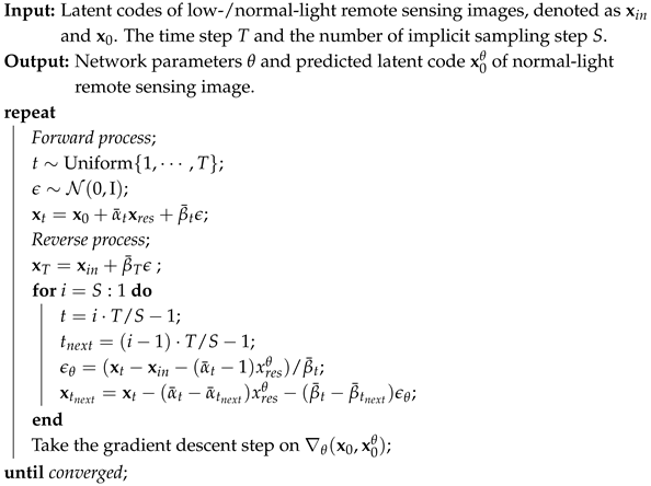
To address this core contradiction, we propose an end-to-end trained single-step diffusion reconstruction mechanism. By reconstructing the training objectives and training process, the diffusion model is made to directly serve the image reconstruction task. Its core design idea is the following: during the training phase, the reverse sampling process of the diffusion model is executed simultaneously, and only the reconstruction loss is used as the optimization objective to achieve task consistency between “training and sampling”.

Diffusion models generally require 50–100 sampling steps [35]. At this time, using the end-to-end training method will greatly prolong the training time. To accelerate the model training, reduce the number of sampling steps, and achieve efficient single-step reconstruction, we introduce the residual diffusion model [20] to replace the standard diffusion model as the core of the model. The residual diffusion model decouples the traditional single denoising diffusion process into a dual diffusion process of residual diffusion and noise diffusion, which provides the possibility for reducing the number of sampling steps and achieving efficient single-step reconstruction.

Forward process: The forward diffusion process of the residual diffusion model involves gradually introducing Gaussian noise and residual terms into the original data, aiming to transform the original data distribution into a noise-added degraded image through a series of minor noise perturbations and residuals. This process can be described as a T-step Markov chain, where each step depends only on the result of the previous step, specifically as follows:

$$q({\mathbf{x}}_1,\dots ,{\mathbf{x}}_T|{\mathbf{x}}_0,{\mathbf{x}}_{res})=\prod _{t=1}^{T}q\left({\mathbf{x}}_t\right|{\mathbf{x}}_{t-1},{\mathbf{x}}_{res}),$$

(8)

$$q\left({\mathbf{x}}_t\right|{\mathbf{x}}_{t-1},{\mathbf{x}}_{res})=\mathcal{N}({\mathbf{x}}_t;{\mathbf{x}}_{t-1}+{\alpha }_t{\mathbf{x}}_{res},{\beta }_t^2\mathbf{I}),$$

(9)

where ${\mathbf{x}}_{res}={\mathbf{x}}_{in}-{\mathbf{x}}_0$, ${\mathbf{x}}_{in}$ is the degraded image, and ${\mathbf{x}}_0$ is the target image. The residual diffusion and noise diffusion are controlled by independent coefficient schedules ${\alpha }_t$ and ${\beta }_t$, respectively, to regulate their diffusion rates. Equation (9) can also be expressed as

$${\mathbf{x}}_t={\mathbf{x}}_{t-1}+{\alpha }_t{\mathbf{x}}_{res}+{\beta }_t{ϵ}_{t-1},$$

(10)

where ${ϵ}_{t-1}\sim \mathcal{N}(\mathbf{0},\mathbf{I})$. Similar to standard diffusion models, ${\mathbf{x}}_t$ at any step can be directly represented by the initial data ${\mathbf{x}}_0$, residuals, and accumulated noise:

$${\mathbf{x}}_t={\mathbf{x}}_0+{\overline{\alpha }}_t{\mathbf{x}}_{res}+{\overline{\beta }}_tϵ,$$

(11)

where $ϵ\sim \mathcal{N}(\mathbf{0},\mathbf{I})$, ${\overline{\alpha }}_t={\sum }_{i=1}^t{\alpha }_i$, and ${\overline{\beta }}_t=\sqrt{{\sum }_{i=1}^t{\beta }_i^2}$. By default, we set $\{{\alpha }_1,{\alpha }_2,\dots ,{\alpha }_T\}$ as a uniformly increasing sequence, and ${\overline{\alpha }}_T=1$; when $t=T$, the endpoint of the forward diffusion process is ${\mathbf{x}}_T={\mathbf{x}}_{in}+{\overline{\beta }}_Tϵ$, which presents the degraded image with random perturbations added.

In the dual diffusion process, the residual diffusion part represents the directional diffusion from the target image to the degraded input image, explicitly providing guidance for the reverse generation process of image restoration. This directionality enables the model to focus more on key information transmission in image restoration tasks and reduces the implicit sampling steps because the degraded image is known, eliminating the need for lengthy reverse processes starting from noise, like standard diffusion models. The noise diffusion, on the other hand, represents random perturbations in the diffusion process. While ensuring the diversity of model outputs, its independent coefficient scheduling mechanism with residual diffusion allows the model to more flexibly balance the needs for determinism and diversity.

Reverse process: The reverse process of the residual diffusion model starts from the degraded image with added random perturbations, gradually reducing the noise and residuals, and ultimately generating a clean target data distribution. If ${\mathbf{x}}_{res}^{\theta }$ are given, where ${\mathbf{x}}_0^{\theta }={\mathbf{x}}_{in}-{\mathbf{x}}_{res}^{\theta }$, the reverse process is defined as

$$p_{\theta }\left({\mathbf{x}}_{0:T}\right)=p\left({\mathbf{x}}_T\right)\prod _{t=1}^T{p}_{\theta }({\mathbf{x}}_{t-1}\mid {\mathbf{x}}_t,{\mathbf{x}}_0^{\theta },{\mathbf{x}}_{res}^{\theta }),$$

(12)

$$p_{\theta }({\mathbf{x}}_{t-1}\mid {\mathbf{x}}_t,{\mathbf{x}}_0^{\theta },{\mathbf{x}}_{res}^{\theta })=\mathcal{N}({\mathbf{x}}_{t-1};{\mathbf{x}}_0^{\theta }+{\overline{\alpha }}_{t-1}{\mathbf{x}}_{res}^{\theta }+\sqrt{{\overline{\beta }}_{t-1}^2-{\sigma }_t^2}{\displaystyle \frac{{\mathbf{x}}_t-({\mathbf{x}}_0^{\theta }+{\overline{\alpha }}_t{\mathbf{x}}_{res}^{\theta })}{{\overline{\beta }}_t}},{\sigma }_t^2\mathbf{I}),$$

(13)

where ${\sigma }_t^2=\eta {\beta }_t^2{\overline{\beta }}_{t-1}^2/{\overline{\beta }}_t^2$, and $\eta =0$ for a deterministic generation process. When $\eta =0$, we can obtain any one-step reverse process:

$${\mathbf{x}}_{t-1}={\mathbf{x}}_t-({\overline{\alpha }}_t-{\overline{\alpha }}_{t-1}){\mathbf{x}}_{res}^{\theta }-({\overline{\beta }}_t-{\overline{\beta }}_{t-1}){ϵ}_{\theta }.$$

(14)

The training objective of the residual diffusion model is to fit a residual prediction model to predict ${\mathbf{x}}_{res}^{\theta }$ by using a U-Net and optimizing the network parameters $\theta$ so as to indirectly obtain ${ϵ}_{\theta }=\left(x_t-x_{in}-({\overline{\alpha }}_t-1)x_{res}^{\theta }\right)/{\overline{\beta }}_t$ from Equation (11), and then calculate ${\mathbf{x}}_{t-1}$ so as to realize the gradual recovery of the original data.

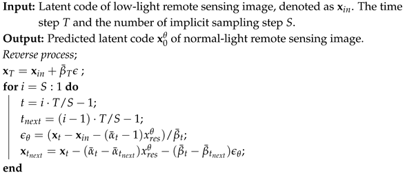
For our end-to-end reconstruction one-step training, following [30], we implement one-step implicit sampling, modify the training objective to indirectly predict ${\mathbf{x}}_0^{\theta }$ through the reverse process, and only calculate the reconstruction loss between ${\mathbf{x}}_0^{\theta }$ and ${\mathbf{x}}_0$. The training and inference processes can refer to Algorithms 1 and 2. Following [36], we use L1 loss and MS-SSIM loss as the reconstruction loss, the objective function is formulated as

$${\mathcal{L}}_{rec}=\left({\mathrm{L}}_1+\mathrm{MS}\text{-}\mathrm{SSIM}\right)({\mathbf{x}}_0,{\mathbf{x}}_0^{\theta }).$$

(15)

Algorithm 1: End-to-end residual diffusion model training.

Algorithm 2: End-to-end residual diffusion model inference.

4.4. Physical Prior Extractor

Although the end-to-end trained single-step diffusion mechanism has significantly improved the efficiency of low-light image enhancement, in practical applications, it is found that the significant reduction in the number of sampling steps will lead to a certain degree of degradation in the model performance. This is because standard multi-step diffusion models gradually correct the generated results through an iterative process. However, in the absence of multi-step iterative correction, single-step diffusion models are prone to structural inconsistencies or illumination anomalies in the generated results due to local-feature-fitting deviations. Especially in low-light images, since the structural information of the original image is inherently blurred, it is more difficult for single-step diffusion models to accurately capture the structural mapping relationship from low light to normal light, which further exacerbates the performance loss.

To address the performance degradation issue in single-step diffusion, we propose an innovative strategy that derives physical priors based on the Kubelka–Munk theory to guide the generation process of the residual diffusion model. The Kubelka–Munk theory describes the spectral energy of light reflected from the surface of an object, and its basic formula is

$$E(\lambda ,x)=e(\lambda ,x)\left({(1-i\left(x\right))}^2{R}_{\infty }(\lambda ,x)+i\left(x\right)\right),$$

(16)

where $\lambda$ denotes the wavelength; x denotes the spatial location; $E(\lambda ,x)$ is the spectral energy of the reflected light; $e(\lambda ,x)$ is the light source spectrum; $i\left(x\right)$ is the specular reflection coefficient; and $R_{\infty }(\lambda ,x)$ is the intrinsic reflectivity of the material, which is only related to material properties and is independent of the illumination.

Through reasonable simplifying assumptions on the above model, illumination-related factors such as the light source spectrum e and specular reflection i can be eliminated, leaving only the intrinsic material property $R_{\infty }$, thereby obtaining the illumination-invariant physical priors.

Assuming that the light source energy is uniform, which means independent of wavelength, $e(\lambda ,x)$ degenerates into $\tilde{e}\left(x\right)$; thus, the model is simplified to

$$E(\lambda ,x)=\tilde{e}\left(x\right)\left({(1-i\left(x\right))}^2{R}_{\infty }(\lambda ,x)+i\left(x\right)\right).$$

(17)

By taking the ratio of the first derivative $E_{\lambda }$ to the second derivative $E_{\lambda \lambda }$ of the spectral energy, i.e., $E_{\lambda }/E_{\lambda \lambda }$, $\tilde{e}\left(x\right)$ and $i\left(x\right)$ can be eliminated, resulting in an illumination invariant S related to $R_{\infty }^{\lambda }/R_{\infty }^{\lambda \lambda }$, that is,

$$S=arctan\left(E_{\lambda }/E_{\lambda \lambda }\right).$$

(18)

Assuming that the object has a diffuse reflection surface, specular reflection is negligible, i.e., $i\left(x\right)\approx 0$; thus, the model is simplified to

$$E(\lambda ,x)=\tilde{e}\left(x\right)R_{\infty }(\lambda ,x).$$

(19)

By taking the ratio of the spectral energy E to its first derivative $E_{\lambda }$, i.e., $E/E_{\lambda }$, $\tilde{e}\left(x\right)$ can be eliminated, resulting in an illumination-invariant C related to $R_{\infty }/R_{\infty }^{\lambda }$, that is,

$$C=arctan\left(E/E_{\lambda }\right).$$

(20)

The last illumination invariant prior is from CIConv [37]. Specifically, under further simplifying assumptions, considering the spectral energy E; its spatial derivatives $E_x$ and $E_y$; and the spatial derivatives $E_{\lambda x}$, $E_{\lambda y}$, $E_{\lambda \lambda x}$, and $E_{\lambda \lambda y}$ of the first-/second-order spectral derivatives $E_{\lambda }$ and $E_{\lambda \lambda }$, the first derived quantities are defined as follows:

$$W_x=E_x/E,W_{\lambda x}=E_{\lambda x}/E,W_{\lambda \lambda x}=E_{\lambda \lambda x}/E.$$

(21)

Similarly, $W_y$, $W_{\lambda y}$, and $W_{\lambda \lambda y}$ can be obtained. On this basis, the illumination invariant W is defined as the gradient magnitude of these derived quantities:

$$W=\sqrt{W_x^2+W_{\lambda x}^2+W_{\lambda \lambda x}^2+W_y^2+W_{\lambda y}^2+W_{\lambda \lambda y}^2},$$

(22)

W can stably reflect the intrinsic edge characteristics of materials without being disturbed by the light intensity, color changes, or specular reflection, thereby achieving robustness against illumination variations:

$$\mathrm{CIConv}={\displaystyle \frac{log\left(W^2+ϵ\right)-{\mu }_{\mathcal{S}}}{{\sigma }_{\mathcal{S}}}},$$

(23)

where $ϵ$ presents a small perturbation, and ${\mu }_{\mathcal{S}}$ and ${\sigma }_{\mathcal{S}}$ refer to the sample mean and standard deviation, respectively.

Our prior extractor is shown in Figure 2. After extracting the prior, we concatenate the prior and inject it as a condition into the U-Net used by the residual diffusion model to guide the model training.

The Gaussian color model is used to estimate the spectral energy and its derivatives from RGB images, providing a basis for the calculation of illumination-invariant physical priors. As a bridge connecting RGB images and spectral energy features, it maps RGB channel values to variables related to spectral energy, such as the spectral energy $\widehat{E}$, first-order spectral derivative ${\widehat{E}}_{\lambda }$, and second-order spectral derivative ${\widehat{E}}_{\lambda \lambda }$, through linear transformation, thereby supporting the derivation of subsequent illumination-invariant priors: S, C, and W. For the input RGB image, the Gaussian color model performs a linear transformation through a 3 × 3 matrix $\mathcal{W}$ with the formula

$$\left[\begin{array}{c}\widehat{E}(x,y)\\ {\widehat{E}}_{\lambda }(x,y)\\ {\widehat{E}}_{\lambda \lambda }(x,y)\end{array}\right]=\left[\begin{array}{ccc}0.06& 0.63& 0.27\\ 0.3& 0.04& -0.35\\ 0.34& -0.6& 0.17\end{array}\right]\left[\begin{array}{c}R(x,y)\\ G(x,y)\\ B(x,y)\end{array}\right],$$

(24)

where $\widehat{E}$ represents the estimated spectral energy; ${\widehat{E}}_{\lambda }$ and ${\widehat{E}}_{\lambda \lambda }$ represent the first-order and second-order spectral derivatives, respectively; and $(x,y)$ is the pixel position. After obtaining $\widehat{E}$, ${\widehat{E}}_{\lambda }$, and ${\widehat{E}}_{\lambda \lambda }$, we calculate E, $E_x$, and $E_y$ by convolving $\widehat{E}$ with Gaussian color smoothing and derivative filters of scale $\sigma$. $\sigma$ is predicted from the input image using three DSConv layers [34]. $E_{\lambda }$, $E_{\lambda x}$, and $E_{\lambda y}$ are calculated from ${\widehat{E}}_{\lambda }$, and $E_{\lambda \lambda }$, $E_{\lambda \lambda x}$, and $E_{\lambda \lambda y}$ are calculated from ${\widehat{E}}_{\lambda \lambda }$. 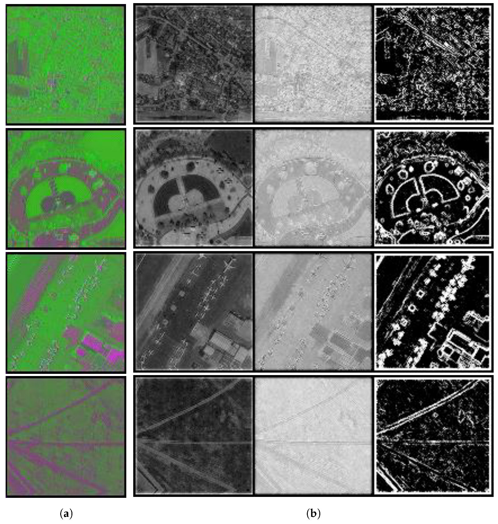The latent codes of normal-light images, along with the priors extracted from their corresponding input images, are shown in Figure 3.

5. Experiments

5.1. Experimental Settings

5.1.1. Datasets and Metrics

Due to the extreme difficulty in obtaining paired data in low-light remote sensing scenarios, following [26,28], we constructed a low-light paired dataset, i.e., dark-iSAID, based on the remote sensing dataset iSAID [38]. This dataset was generated by simulating light variations in low-illumination environments and adding appropriate noise to simulate dark-region noise and sensor noise. Meanwhile, we validated the effectiveness of the proposed method on the real-scene low-light remote sensing dataset Darkrs. These datasets have been widely used in research related to remote sensing image enhancement [27,38].

To further evaluate the generalization ability of the model for low-light images in different real scenarios, we additionally selected several well-recognized datasets for testing, including DICM [39], NPE [40], LIME [41], and LSRW [42]. The datasets used in the experiments cover both remote sensing and non-remote sensing fields, including natural outdoor scenes and typical indoor environments. Among them, non-remote sensing datasets (such as aerial sky images and low-light indoor scenes) can further verify the generalization performance of the algorithm.

In addition, the datasets can be divided into two categories: paired and unpaired, and a comprehensive comparison was conducted using multi-dimensional evaluation metrics. For the paired datasets, full-reference metrics were adopted: Peak Signal-to-Noise Ratio (PSNR), Structural Similarity Index (SSIM) [43], Learned Perceptual Image Patch Similarity (LPIPS) [44], and Mean Absolute Error (MAE). For the unpaired datasets, no-reference metrics were adopted: Natural Image Quality Evaluator (NIQE) [45], Blind/Referenceless Image Spatial Quality Evaluator (BRISQUE) [46], Perceptual Image Quality Evaluator (PIQE) [47], and Noise Level (NL) [48].

5.1.2. Implementation Details

The proposed method was implemented based on Pytorch [49], and all comparative experiments were conducted on a system equipped with an NVIDIA RTX 4090 graphics card.

During the training process, the lightweight encoder–decoder and the end-to-end single-step latent residual diffusion model were trained separately, with independent Adam optimizers [50] configured for each. Both optimizers had an initial learning rate of $8\times {10}^{-5}$, and the momentum parameter was uniformly set to (0.9, 0.999). During training, $512\times 512$ image patches were randomly cropped and input into the model; in the inference phase, the length and width of the image were first reflectively padded to multiples of 64, and after the enhancement, the results were cropped back to the original size.

The time step T in the training phase was set to 1000, while the implicit sampling step S was set to 1 in both the training and inference phases. We set the noise coefficients $\{{\beta }_1^2,{\beta }_2^2,\dots ,{\beta }_T^2\}$ in the residual diffusion model as a uniformly decreasing sequence, and ${\overline{\beta }}_T=1$. We set different hyper-parameters for the U-Net used in the end-to-end residual diffusion model, dividing it into four versions:

• Ours-T: C = 32, channel multiplier = 1, 1, 1, 1;
• Ours-S: C = 32, channel multiplier = 1, 2, 2, 4;
• Ours-M: C = 64, channel multiplier = 1, 2, 2, 4;
• Ours-L: C = 64, channel multiplier = 1, 2, 4, 8.

where C is the number of channels in the first hidden layer. The parameters of each version are 0.89 M, 3.27 M, 12.41 M, and 36.26 M (excluding the encoder–decoder).

5.2. Comparison of the Encoder–Decoder

To verify the role of our lightweight encoder–decoder dedicated to the low-light remote sensing field, we validated the reconstruction efficiency and performance of our encoder–decoder with three encoders–decoders in an LDM (4× compression, 8× compression, and 16× compression) on the dark-iSAID and darkrs datasets. The encoders–decoders in the LDM infer by default at a size of $256\times 256$ pixels, so we also conducted experiments at this size. We report the model parameters, average reconstruction time, and PSNR and SSIM metrics on the normal-light test set of dark-ISAID in

Table 1. Quantitative comparison of the encoder–decoder. The best results are highlighted in bold.

Method	Params (M)	Time (s)	PSNR↑	SSIM↑
LDM 4×↓	72.793	0.9584	28.498	0.828
LDM 8×↓	101.136	0.7134	24.524	0.655
LDM 16×↓	87.094	0.3802	24.343	0.640
Ours 8×↓	5.914	0.0035	30.854	0.891

. We also show visual comparison in Figure 4. As shown in the table, our encoder–decoder has significantly fewer parameters, only 5.914 M, while the LDM encoder–decoder has a minimum of 72.793 M. Meanwhile, its reconstruction time is extremely short, only 0.0035 s, achieving a 203× speedup at the same compression ratio. In terms of the performance metrics, its PSNR (30.854) and SSIM (0.891) are much higher than even LDM 8×↓, and even higher than LDM 4×↓, indicating that our method has advantages in both efficiency and reconstruction quality.

In terms of visual comparison, for LDM with 4× compression, there are slight deviations from the ground truth, yet still retains a certain level of structural similarity. As the compression level of LDM increases to 8× and 16×, the visual degradation becomes more apparent. Details in the highlighted regions become blurred; edges become less distinct; and there is a noticeable loss of fine textures, especially in complex structures like buildings and vegetation boundaries. In contrast, our method shows a remarkable improvement in visual fidelity. The details, colors, and brightness are much better preserved, presenting a more natural and accurate visual reconstruction, which further validates the superiority of our lightweight encoder–decoder in low-light remote sensing image processing.

5.3. Comparison with the State-of-the-Art Methods

In this section, we conducted both quantitative and qualitative comparative evaluations to assess the effectiveness of our proposed method against several state-of-the-art (SOTA) methods in the field of low-light remote sensing image enhancement. The comparative methods were Zero-DCE [51], RUAS [52], SCI [53], URetinexNet [22], Uformer [12], CLIP-LIT [54], PairLIE [23], NeRCo [24], GPP-LLIE [55], and LIEDNet [25].

For the dark-iSAID dataset, quantitative results in

Table 2. Quantitative results on the dark-iSAID test set. The best results are highlighted in bold.

Method	PSNR↑	SSIM↑	LPIPS↓	MAE↓
Zero-DCE	16.492	0.309	0.766	31.759
RUAS	12.382	0.287	0.797	56.980
SCI	16.351	0.299	0.789	32.999
URetinexNet	18.541	0.461	0.699	26.236
Uformer	26.252	0.692	0.363	9.478
CLIP-LIT	13.732	0.272	0.863	46.047
PairLIE	20.454	0.612	0.445	19.993
NeRCo	21.421	0.622	0.411	18.127
GPP-LLIE	19.605	0.602	0.559	23.591
LIEDNet	26.121	0.629	0.387	9.450
Ours-T	26.402	0.755	0.353	9.453
Ours-S	26.354	0.766	0.326	9.689
Ours-M	26.379	0.771	0.327	9.618
Ours-L	26.838	0.776	0.318	9.044

demonstrate the superiority of our proposed methods across four metrics (PSNR, SSIM, LPIPS, MAE). Among our methods, Ours-L achieves the best performance, its PSNR reaches 26.838, outperforming the second-best method Uformer (26.252) by 0.586; the SSIM hits 0.776, leading Uformer (0.692) by a large margin (0.084); the LPIPS is 0.318, the lowest across all methods and indicating minimal perceptual difference; the MAE is 9.044 better than LIEDNet (9.450). Other variants (Ours-T, Ours-S, Ours-M) also show competitive results, with PSNR values ranging from 26.354 to 26.402, the SSIM from 0.755 to 0.771, the LPIPS from 0.326 to 0.353, and the MAE from 9.453 to 9.689. Overall, our method series comprehensively surpasses state-of-the-art (SOTA) methods like Uformer and LIEDNet in restoring image signals, structural integrity, perceptual quality, and pixel details, providing a more accurate solution for low-light remote sensing image enhancement.

Visual comparisons shown in Figure 5 further highlight the advantages of our method. Methods such as Uformer, CLIP-LIT, PairLIE, NeRCo, GPP-LLIE, and LIEDNet have limitations. Uformer suffers from color distortion and an overall dark frame; CLIP-LIT and PairLIE fail to completely eliminate noise, with a large amount of residual noise in the zoomed-in sections; NeRCo and GPP-LLIE exhibit uneven brightness and an overall whitish tone in the frame; and LIEDNet has the issue of detail loss, where building textures and vehicle shapes appear blurred or distorted. In contrast, our method effectively suppresses noise, accurately restores colors and details, balances noise removal and detail enhancement, clearly presents targets such as buildings and vehicles, and achieves a uniform brightness distribution—thus providing excellent visual quality for low-light image enhancement on the dark-iSAID dataset.

We further evaluated the methods on the darkrs dataset across the NIQE, BRISQUE, PIQE, and NL metrics. As shown in

Table 3. Quantitative results from Figure 6. The best results are highlighted in bold.

Method	NIQE↓	BRISQUE↓	PIQE↓	NL↓
Zero-DCE	3.516	42.372	12.423	0.418
RUAS	6.139	47.578	17.565	2.783
SCI	3.814	48.798	16.666	0.566
URetinexNet	4.961	35.907	12.937	1.634
Uformer	4.964	32.569	13.246	0.518
CLIP-LIT	5.603	49.232	17.878	1.052
PairLIE	3.341	21.979	8.155	0.404
NeRCo	3.313	28.694	7.813	0.718
GPP-LLIE	3.504	32.562	7.587	0.282
LIEDNet	6.365	17.799	6.884	0.487
Ours	2.706	13.976	6.748	0.315

, our method achieves an NIQE score of 2.706, substantially lower than the second-best competitor NeRCo (3.313), and a BRISQUE score of 13.976, outpacing the second-best method LIEDNet (17.799), which showcases superior perceptual quality. The PIQE score reaches 6.748, standing out against LIEDNet (6.884), and the NL score reaches the second-best result of 0.315.

For the visual results shown in Figure 6, the brightness enhanced by NeRCo and GPP-LLIE is insufficient, resulting in an overall dark frame. LIEDNet loses details and distorts colors during the enhancement process. In contrast, our method effectively suppresses the noise, uniformly enhances the brightness, and accurately restores the scene details and colors. It clearly highlights building textures and road details, achieving a visual effect that far surpasses other methods.

We further evaluated the performance in non-remote sensing scenarios to assess the robustness of our method. For unpaired datasets (DICM, NPE, and LIME), as shown in

Table 4. Quantitative results from Figure 7. The best results are highlighted in bold.

Method	NIQE↓	BRISQUE↓	PIQE↓	NL↓
Zero-DCE	2.730	16.671	11.476	0.847
RUAS	4.562	37.752	11.607	4.296
SCI	3.022	16.799	12.068	2.145
URetinexNet	2.781	16.433	11.791	2.095
Uformer	4.157	28.417	12.256	4.397
CLIP-LIT	2.987	18.249	13.471	1.874
PairLIE	3.470	18.202	7.919	0.645
NeRCo	2.974	18.766	7.121	1.108
GPP-LLIE	3.830	21.588	16.083	0.402
LIEDNet	4.851	25.490	6.086	0.798
Ours	2.479	16.363	8.829	0.386

, our method achieves scores of 2.479, 16.363, and 0.386 in the NIQE, BRISQUE, and NL, respectively, outperforming the second-best methods Zero-DCE (2.730) in the NIQE, URetinexNet (16.433) in the BRISQUE, and GPP-LLIE (0.402) in the NL. Visual comparisons in Figure 7 indicate that Zero-DCE and URetinexNet leave a large amount of residual noise; while GPP-LLIE can effectively remove noise, it may introduce color distortion. In contrast, our method performs excellently across all scenarios, and it clearly presents elements such as tree textures, building details, and facilities in outdoor scenes.

For the paired dataset (LSRW), the results are presented in

Table 5. Quantitative results on LSRW test set. The best results are highlighted in bold.

Method	PSNR↑	SSIM↑	LPIPS↓	MAE↓
Zero-DCE	15.858	0.454	0.318	35.895
RUAS	13.024	0.359	0.379	52.044
SCI	15.232	0.424	0.328	39.271
URetinexNet	18.271	0.526	0.299	25.208
Uformer	14.160	0.502	0.511	44.260
CLIP-LIT	13.473	0.409	0.357	47.459
PairLIE	17.602	0.512	0.329	27.939
NeRCo	17.844	0.545	0.375	27.933
GPP-LLIE	17.594	0.535	0.302	28.588
LIEDNet	18.877	0.545	0.450	24.284
Ours-T	19.101	0.570	0.460	23.707
Ours-S	19.170	0.571	0.462	23.653
Ours-M	19.375	0.576	0.397	22.818
Ours-L	19.420	0.576	0.366	22.187

and Figure 8. Quantitatively, Ours-L achieves the highest values in the PSNR and SSIM, which are 19.420 and 0.576, respectively, surpassing the second-best methods by 0.543 and 0.031, respectively. It also attains the lowest MAE score of 22.187, which is superior to the second-best method LIEDNet (24.284). Qualitatively, NeRCo poorly integrates brightness and color, and LIEDNet fails to restore fine details. In contrast, our method effectively suppresses noise, accurately restores colors and fine details (such as wood color and text details), and ensures a uniform and natural brightness distribution, leading to visual effects that comprehensively outperform comparative methods.

5.4. Computational Complexity

In addition to the enhancement performance, the computational efficiency is also important in the field of low-light remote sensing image enhancement. We evaluate the computational costs of various methods using the inference times (s) under different input resolutions ($512\times 512$, $800\times 800$, $1024\times 1024$, and $1500\times 1500$), and the results are summarized in

Table 6. Inference times (s) under different resolutions. The best results are highlighted in bold.

Method	$512\times 512$	$800\times 800$	$1024\times 1024$	$1500\times 1500$
URetinexNet	0.0155	0.0471	0.0782	0.1724
Uformer	0.0726	0.2240	0.2921	0.6554
PairLIE	0.0267	0.0692	0.0972	0.2354
NeRCo	0.1620	0.4519	0.6807	-
GPP-LLIE	0.6901	1.7661	-	-
LIEDNet	0.0535	0.1224	0.2078	0.5173
Ours-T	0.0335	0.0466	0.0584	0.1098
Ours-S	0.0339	0.0469	0.0621	0.1103
Ours-M	0.0351	0.0479	0.0658	0.1119
Ours-L	0.0353	0.0481	0.0681	0.1192

. When comparing competing methods with the methods proposed in this paper, namely, Ours-T, Ours-S, Ours-M, and Ours-L, a shorter inference time indicates lower computational complexity. It should be noted that some inference times are unavailable due to out-of-memory (OOM) issues.

Specifically, at the $512\times 512$ resolution, the CNN-based URetinexNet achieves an inference time of 0.0155, which is the lowest among the compared methods. Among our proposed methods, Ours-T, with an inference time of 0.0335, is competitive when compared with some of the other methods (such as NeRCo with 0.1620 and LIEDNet with 0.0535). As the resolution increases to $800\times 800$, $1024\times 1024$, and $1500\times 1500$, our methods consistently achieve the lowest inference times, which are 0.0466, 0.0584, and 0.1098, respectively. These results outperform those of the CNN-based methods (URetinexNet and PairLIE), Transformer-based method (Uformer), implicit-neural-representation-based method (NeRCo), Mamba-based method (LIEDNet), and diffusion-based method (GPP-LLIE). As a diffusion-model-based method, our approach (0.0335) achieves approximately 20× faster inference speed than GPP-LLIE (0.6901). This indicates that our methods have great application potential for large-sized remote sensing images.

5.5. Ablation Studies

To assess the effectiveness of several key components in our proposed method, we conducted a series of ablation studies. All ablation experiments were performed using the dark-iSAID dataset. As shown in

Table 7. Ablation studies on the design effectiveness of our method. “w/o” indicates without.

Method		PSNR↑	SSIM↑	LPIPS↓
Training	w/o end-to-end, L1 loss	25.110	0.644	0.441
	w/o end-to-end, L2 loss	24.868	0.671	0.405
	w/o end-to-end	26.003	0.659	0.406
Steps and Noise	$S=1$, ${\overline{\beta }}_T=0.1$	26.665	0.780	0.302
	$S=2$, ${\overline{\beta }}_T=0.1$	26.642	0.777	0.297
	$S=5$, ${\overline{\beta }}_T=0.1$	26.964	0.770	0.331
	$S=2$, ${\overline{\beta }}_T=1$	26.762	0.779	0.306
	$S=5$, ${\overline{\beta }}_T=1$	27.111	0.781	0.306
Physical Priors	w/o S	26.293	0.758	0.340
	w/o C	26.181	0.756	0.348
	w/o W	25.805	0.768	0.336
Default Version		26.838	0.776	0.318

, our default setting is highlight in bold.

5.5.1. End-to-End Training

To verify the effectiveness of our end-to-end trained residual diffusion model, we conducted an ablation experiment using the standard diffusion model training method (w/o end-to-end). Specifically, we no longer synchronously execute the sampling process of the diffusion model during the training phase, so that the residual diffusion model no longer directly serves the reconstruction task. Instead, it focuses on using the U-Net to predict the residuals and noise that need to be removed at each step. Our training objective is updated to ${\mathcal{L}}_{diff}=\left({\mathrm{L}}_1+\mathrm{MS}\text{-}\mathrm{SSIM}\right)({\mathbf{x}}_{res},{\mathbf{x}}_{res}^{\theta })$, furthermore, we also tested variants with only L1 loss (w/o end-to-end, L1 loss) and only L2 loss (w/o end-to-end, L2 loss).

From Table 7, the PSNR of “w/o end-to-end” (26.003) is lower than that of the default version (26.838), and its SSIM (0.659) and LPIPS (0.406) are also less optimal. The L1 loss variant has a PSNR of 25.110, and the L2 loss variant has a PSNR of 24.868, both significantly lower than the end-to-end training. The visual and metric comparisons on a single image are presented in Figure 9. All of these show that the end-to-end training mechanism helps the model better fit the task, enabling the residual diffusion model to more effectively contribute to image reconstruction, and the combined L1 + MS-SSIM loss is more beneficial for performance improvement compared with using a single loss.

5.5.2. Sampling Steps and Noise Coefficient

In the experimental settings of Section 5.1.2, we set the number of implicit sampling steps S to 1, the coefficient sequence $\{{\beta }_1^2,{\beta }_2^2,\dots ,{\beta }_T^2\}$ of the noise diffusion process to decrease uniformly, and ${\overline{\beta }}_T=1$. We conducted ablation experiments to evaluate the impact of different S and ${\overline{\beta }}_T$. Specifically, we further tried combinations of implicit sampling steps S of 2 and 5, and ${\overline{\beta }}_T$ of 0.1.

The results in Table 7 show that when the number of S increases from 1 to 2 and then to 5, the model’s performance in various metrics only fluctuates slightly, the variation range of PSNR values does not exceed 0.349 dB, the fluctuation of SSIM values is controlled within 0.005, and the difference in LPIPS values is also less than 0.012. This phenomenon benefits from the end-to-end training mechanism and physical prior guidance we adopted. End-to-end training enables the model to directly serve the reconstruction task, while physical priors provide a stable guidance framework, thus ensuring the robustness of the model’s performance. Meanwhile, it can be found that the differences under the two settings (${\overline{\beta }}_T=0.1$, ${\overline{\beta }}_T=1$) are also small. This indicates that under the guidance of physical priors, the model has strong adaptability to changes in noise coefficients, and the specific values of noise coefficients will not significantly affect its processing effect on low-light image enhancement tasks.

5.5.3. Physical Priors

Finally, we analyzed the role of each illumination-invariant physical prior. In the experiment, we separately removed each of the three priors ($S,C,W$) introduced in the model and observed the changes in the various metrics one by one.

As shown in Table 7, the PSNRs of “w/o S” is 26.293, “w/o C” is 26.181, and “w/o W” is 25.805, all of which are lower than the default version (26.838). Their SSIM and LPIPS also show worse performances compared with the default. This demonstrates that each component of the physical priors plays a positive role in the model. The visual and metric comparisons on a single image are presented in Figure 10. The integration of these priors helps the model better conform to the physical characteristics of images during the enhancement process, thereby improving the overall quality of low-light remote sensing image enhancement.

6. Discussion

The proposed framework integrates a lightweight encoder–decoder, an end-to-end trained single-step residual diffusion model, and illumination-invariant physical priors. Its design addresses critical challenges in existing methods, particularly in balancing efficiency and performance.

The dedicated lightweight encoder–decoder stands out by targeting the unique characteristics of low-light remote sensing scenes. Unlike general-purpose encoders–decoders that often carry redundant computations and struggle to preserve subtle features in dim environments, this tailored component efficiently compresses and reconstructs information. This adaptability to low-light feature distributions lays a solid foundation for subsequent diffusion-based enhancement.

The end-to-end trained single-step residual diffusion model redefines the efficiency of diffusion models in this domain. By abandoning the multi-step noise estimation paradigm, it streamlines the enhancement pipeline without compromising quality. This is crucial for remote sensing tasks, where rapid processing of large-volume imagery is essential. The mechanism’s success highlights that diffusion models can be optimized for practical speed requirements when aligned with task-specific goals.

The integration of illumination-invariant priors addresses a long-standing issue in low-light processing of ambiguity from missing details. By imposing structural guidance rooted in physical properties, the framework reduces generation blurriness and enhances robustness across varying low-light conditions. This physics-informed guidance bridges the gap between data-driven learning and domain knowledge, demonstrating that incorporating prior knowledge can significantly stabilize and improve model performance.

Comparisons with mainstream methods underscore the framework’s superiority in both quantitative metrics (e.g., PSNR and SSIM shown in Figure 11) and visual quality. However, it is important to note that the framework’s performance may vary in extreme low-light conditions, as the priors rely on at least minimal residual information to guide the enhancement. In addition, in some scenarios where there is a large gap between bright and dark areas, the model may experience partial overexposure. Future work could explore fixing these issues and extending this method to low-light enhancement of multispectral remote sensing images.

7. Conclusions

In conclusion, this study presents a robust and efficient framework for low-light remote sensing image enhancement, with four key contributions. First, the lightweight encoder–decoder, tailored to low-light remote sensing scenes, reduces computational redundancy while preserving critical features. Second, the end-to-end trained single-step residual diffusion model accelerates inference significantly, enabling fast processing without sacrificing quality. Third, illumination-invariant priors provide structural guidance, mitigating blurriness from missing details and enhancing robustness in complex environments. Finally, extensive experiments on multiple datasets validate the framework’s superiority over mainstream methods, confirming its practical value.

This work balances speed, accuracy, and perceptual quality in low-light remote sensing image enhancement, the framework meets the demands of real-world remote sensing applications, where both efficiency and reliability are paramount. Future research could focus on extending the framework to handle ultra-low-light scenarios and general image restoration tasks, further broadening its impact in remote sensing and related fields.