Assessing the Robustness of Multispectral Satellite Imagery with LiDAR Topographic Attributes and Ancillary Data to Predict Vertical Structure in a Wet Eucalypt Forest

Abstract

Remote sensing approaches can be cost-effective for estimating forest structural attributes. This study aims to use airborne LiDAR data to assess the robustness of multispectral satellite imagery and topographic attributes derived from DEMs to predict the density of three vegetation layers in a wet eucalypt forest in Tasmania, Australia. We compared the predictive capacity of medium-resolution Landsat-8 Operational Land Imager (OLI) surface reflectance and three pixel sizes from high-resolution WorldView-3 satellite imagery. These datasets were combined with topographic attributes extracted from resampled LiDAR-derived DEMs and a geology layer and validated with vegetation density layers extracted from high-density LiDAR. Using spectral bands, indices, texture features, a geology layer, and topographic attributes as predictor variables, we evaluated the predictive power of 13 data schemes at three different pixel sizes (1.6 m, 7.5 m, and 30 m). The schemes of the 30 m Landsat-8 (OLI) dataset provided better model accuracy than the WorldView-3 dataset across all three pixel sizes (R² values from 0.15 to 0.65) and all three vegetation layers. The model accuracies increased with an increase in the number of predictor variables. For predicting the density of the overstorey vegetation, spectral indices (R² = 0.48) and texture features (R² = 0.47) were useful, and when both were combined, they produced higher model accuracy (R² = 0.56) than either dataset alone. Model prediction improved further when all five data sources were included (R² = 0.65). The best models for mid-storey (R² = 0.46) and understorey (R² = 0.44) vegetation had lower predictive capacity than for the overstorey. The models validated using an independent dataset confirmed the robustness. The spectral indices and texture features derived from the Landsat data products integrated with the low-density LiDAR data can provide valuable information on the forest structure of larger geographical areas for sustainable management and monitoring of the forest landscape.

1. Introduction

Vertical forest structure (VFS) is an essential component of ecological processes [1] habitat quality and biodiversity [2,3]. VFS is the vertical stratification or layering of a forest [1] and for this study, refers to the density of vegetation in each of three layers of the forest: understorey, mid-storey and overstorey. Knowledge about VFS is helpful in relation to timber production and carbon sequestration [4,5,6], the habitat requirements of different organisms [7], and the distribution of fuels and fire behaviour [8,9,10]. Detailed knowledge of VFS is required to manage forests for estimating forest water storage capacity [11], wildlife habitat management, wildfire mitigation [4,10,12,13], and understanding habitat restoration plans [14]. However, measuring VFS directly in the field is an ongoing challenge for forest managers [15] and is expensive, time-consuming, and logistically difficult [1,16] The assessment of vertical vegetation structure is a key component in monitoring terrestrial ecosystems [17], where the density of vegetation strata plays a crucial role in providing a suitable habitat for biodiversity and understanding ecosystem processes [18]. The understorey, mid-storey and overstorey vegetation typically provide varied habitats and light conditions, supporting different plant and animal species. In primary forests, the history and severity of previous natural disturbances like wildfires, and local factors like underlying geology and soil properties, moisture availability, elevation and topography, all influence the VFS. Ecologically meaningful and robust measures of VFS for remote, inaccessible, and large geographical areas have been lacking [3,19] and require further research, in particular for sub-canopy metrics [4].

Remote Sensing satellite data have been used for modelling and mapping forest structural attributes in large geographical areas [1,20,21]. Mapping forest structure attributes using remotely sensed data has been a topic of research for over four decades [20,22]. Although aerial photographs were previously used for mapping forest stands, those techniques were highly subjective, time-consuming, and depended on the experience of the interpreter [22,23]. With the advancements in technologies, automated image analysis techniques were explored to retrieve forest stand structural attributes [22]. Satellite imagery was found to meet the needs of spatially contiguous information about the canopy surface of forests over large geographical areas [24,25], but had limited capacity to describe sub-canopy conditions.

Although traditional passive remote sensing techniques have demonstrated the potential to provide useful information on forest structure attributes based on spectral reflectance and derived vegetation indices [26], these techniques are not currently sufficient to predict and map three-dimensional (3D) VFS for forestry and ecological applications [27] Also, the successful application of remote sensing data depends on identifying the optimum spatial resolution [28] for monitoring multiscale biodiversity attributes [29]. To date, the assessment of optimum spatial resolution remains an area of active research, especially for heterogeneous ecosystems [30]. As an alternative to passive remote sensing techniques, Light Detection and Ranging (LiDAR), an active remote sensing technology, can directly measure the 3D vegetation structure characteristics by penetrating through canopy gaps [4,31,32,33,34] and provide valuable information on VFS for ecological and forestry applications [1,34,35]. LiDAR sensor platforms can be spaceborne, airborne, and terrestrial, with their specific advantages, limitations and observation scales [36]. The VFS is one of the six essential biodiversity variable classes affecting species distributions and diversity by providing food, habitat, and nesting sites [35]. LiDAR point clouds can be used to extract detailed information on vegetation structural characteristics, including vegetation arrangement, structural complexity, canopy cover, leaf area, and density [37].

This technology has been widely used in ecological studies [38] and provides a valuable tool in forest inventory [8,9,39]. In addition, LiDAR has been used for the assessment of structural response to a range of bushfire events [12,40], wildlife-habitat relationships [41], and bird species richness [42,43]. LiDAR is the most popular approach to survey VFS and can bridge the gap between satellite and field data [44,45]. The increasing capabilities of LiDAR technology allow researchers to characterise forest structure [1,43] and could also be used to quantify structural diversity at multiple scales [46].

LiDAR can capture VFS even in high-biomass forests, where optical multispectral satellite data tend to be saturated [20,47,48] and cannot provide information about the vegetation layers underneath the canopy cover [49]. Although LiDAR point clouds can capture VFS, their application to large geographical areas is challenging due to logistical, cost, and data volume constraints [44]. High-resolution LiDAR is likely to be cost-prohibitive for broadscale applications. So, there is considerable interest by natural resource managers and the forest industry in integrating operational resolution LiDAR and multispectral satellite data to retrieve forest structural attributes [8,15,50]. Considering the different aspects of VFS, no single sensor can exhibit all the required information relevant to forest managers, and the integration of multispectral satellite imagery and LiDAR data could advance the prediction and mapping of forest structure characteristics [47].

Topography plays a significant role in the development of VFS, affecting abiotic conditions, i.e., microclimate and edaphic factors [51,52] that can influence the structure, function, and dynamics of ecological communities [51]. Topographic attributes provide a basis for understanding ecological relationships with vegetation, landforms, and soils [53], and are important drivers for various local and regional geodynamic processes [54]. Spectral vegetation indices are broadly used for estimating various biophysical and biochemical properties of vegetation.

There is relatively limited research into predicting VFS from LiDAR-derived topographic attributes with other sources of remote sensing satellite data, especially in mixed-species forests [8,55]. Due to the complex forest structure as well as topographic variations, stratifying a complex forest over a large geographical area is still challenging [56]. This study aims to evaluate the robustness of predicting the density at three vertical forest layers in a wet eucalypt forest (Tasmania, Australia) based on multispectral satellite imagery combined with topographic attributes derived from a digital elevation model (DEM). Moreover, this study assesses whether selected vegetation indices and image texture features improve the prediction accuracy of the VFS attributes. To provide insights into the different sources of datasets owing to different scales, this study examines the importance of predictor variables and investigates how three different pixel sizes influence model outcomes. Thus, this study addresses data complexities, including multidimensionality and nonlinearity in multisource data, and provides a robust approach for assessing forest structure.

2. Materials and Methods

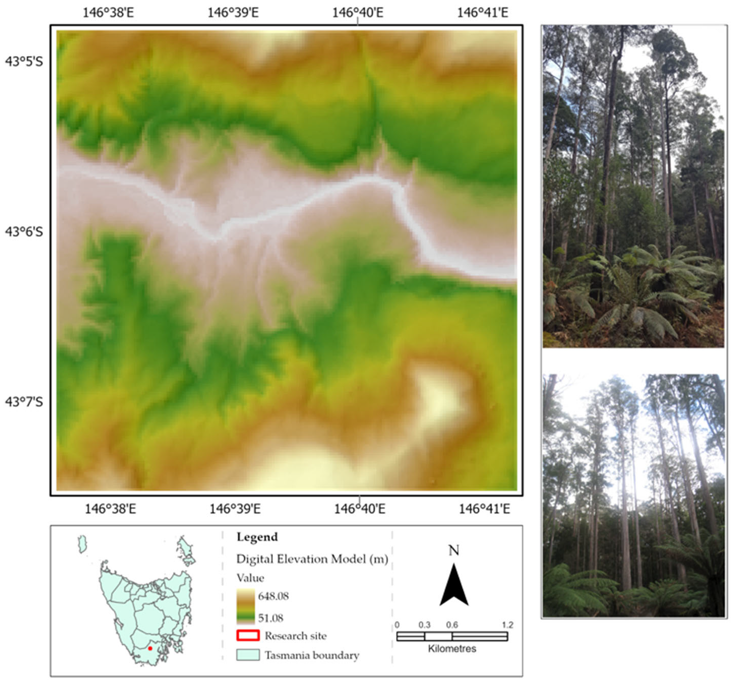
2.1. Study Site

We conducted this research within a 5 km by 5 km area centred at 43.104°S and 146.656°E, located at the Warra Supersite within the Tasmanian World Heritage Area, Australia. The selected site (Figure 1) is topographically and geologically complex, comprising forests ranging from 1934 wildfire regrowth through to old-growth, rivers, gullies and ridges. The ground elevation ranges from 51 m to 648 m above mean sea level according to the 30 m resolution DEM. The Warra site is a member of the Terrestrial Ecosystem Research Network (TERN) Australian Supersite Network [57], which covers the cool, temperate wet forest biome. Mean annual rainfall is 1707 mm, and mean daily temperature ranges are 8.3 °C to 19.3 °C in January (summer) and 2.5 °C to 8.6 °C in July (winter) [58].

The Warra Supersite is one of the most productive terrestrial ecosystems in the world, and its management generates a high level of political and social interest. This Supersite has a long history of fire, with several fires since 1850, and ranges from intensively managed to protected forests [59]. There is a general pattern of ecological succession from wet sclerophyll-dominated younger stands to older mixed forests consisting of eucalypts with a rainforest understorey [60]. The forest at the study site is mostly dominated by Eucalyptus obliqua, which forms a tall (~50 m) overstorey overtopping secondary stratum of trees, for example, Acacia dealbata and Acacia melanoxylon, or rainforest trees such as Nothofagus cunninghamii, Atherosperma moschatum and Eucryphia lucida. Understorey tree and shrub species vary from dense Melaleuca squarrosa and Leptospermum lanigerum on soils with impeded drainage to Nematolepis squamea and Pomaderris apetala on well-drained soils [61]. The understorey includes tree ferns (Dicksonia antarctica), Bauera rubioides, the tall sedge Gahnia grandis, and other understorey shrubs and trees of up to ~10 m in height.

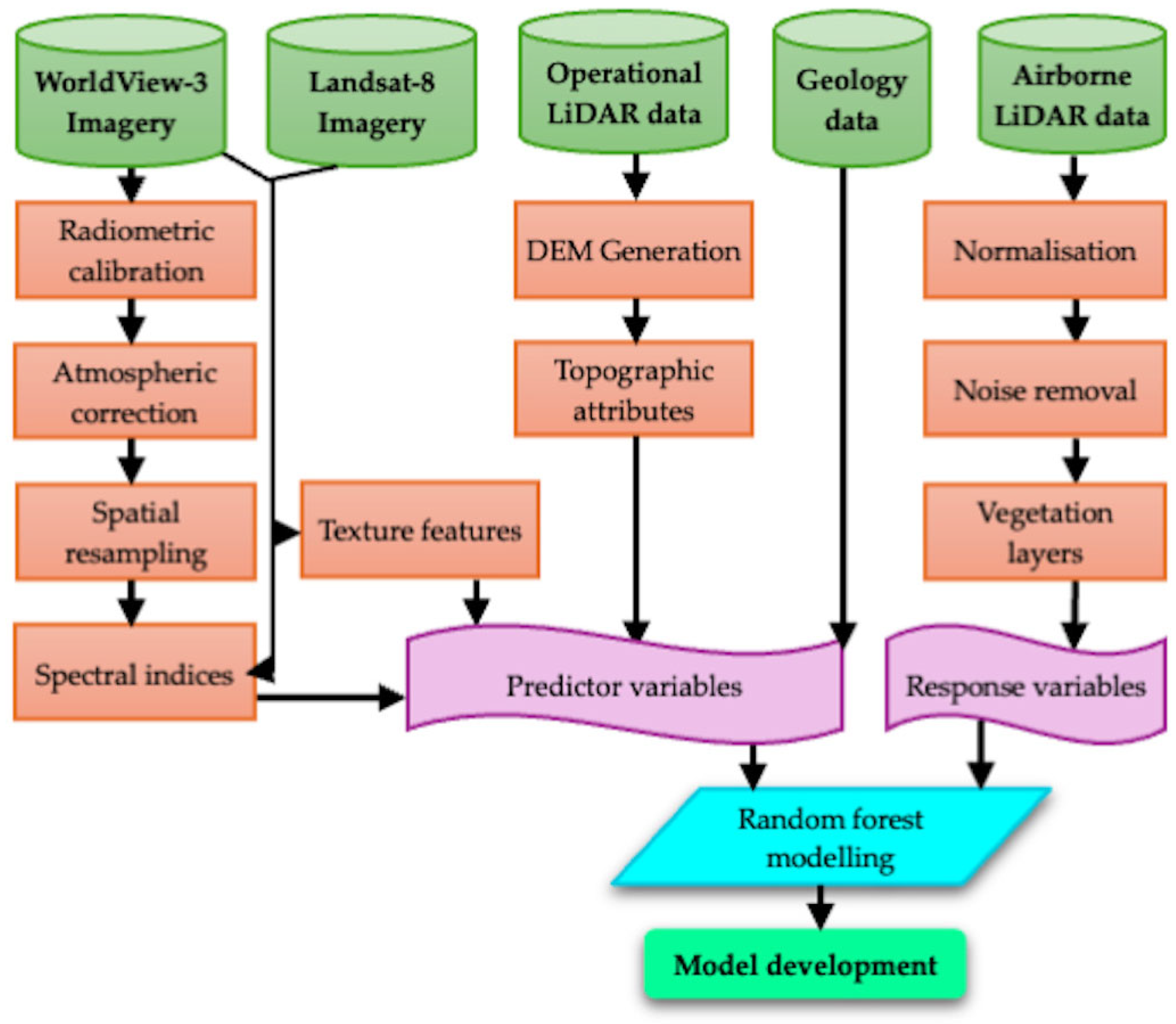
2.2. Remote Sensing Data

We used airborne LiDAR point clouds in combination with WorldView-3 and Landsat-8 (OLI) satellite multispectral remote sensing datasets and ancillary data, i.e., a geology map layer [62]. Airborne LiDAR data used in this study was collected by Airborne Research Australia using a Riegl LMS-Q560 laser sensor on Diamond Aircraft HK36TTC ECO-Dimonas. LiDAR data with a spatial resolution of 28.66 points m⁻² (horizontal spacing = 0.19 m) and a 1064 nm laser wavelength was collected from a flying height of 500 m above terrain on 30 May 2014. The scan angle rank ranged from −360 to 44°. Full-waveform data were collected and discretised up to 7 returns per pulse. The scale factor of the data was 0.01 m.

In this study, the discrete return airborne LiDAR data of 28.66 points m⁻² were thinned to reduce the point density to 4.94 points m⁻² and spacing of 0.45 m (all returns) to simulate operational low-density LiDAR data typically available to management agencies for forest surveys. The high-resolution data were used for generating response variables (density of three vegetation strata) and the thinned operational LiDAR data to generate topographic attributes for predictor variables. We assume that 28.66 points m⁻² is sufficient to obtain an accurate estimation of vegetation structure, as many European countries consider point density more than 4 points m⁻² can produce accurate estimates of vegetation structure at 10 m spatial resolution [63,64], and even lower density data can be used as a basis for modelling [35].

This study did not consider field plot data, which were unavailable; thus, we used an approach solely depending on remote sensing data, simulating operational LiDAR data from high-density LiDAR data for predicting VFS. WorldView-3 satellite imagery acquired on 5 October 2015 was resampled from 1.6 m pixel size for the visible near-infrared (VNIR) 8 bands to 7.5 m using pixel aggregation [65] to match the spatial resolution of the shortwave infrared (SWIR) 8 bands of the same WorldView-3 imagery. We then used all 16 bands for further analysis. Similarly, all 16 bands of WorldView-3 imagery were again resampled to 30 m pixels to match the spatial resolution of the Landsat 30 m (OLI) data acquired on 21 October 2014 (See

Table 1. Specifications of multispectral remote sensing datasets.

Specification Item	WorldView-3 Imagery	Landsat-8 Imagery
Date of acquisition	5 October 2015	21 October 2014
Spatial resolution	1.60 m (VNIR bands) 7.50 m (SWIR bands)	30 m (VNIR and SWIR bands)
Sun azimuth	42.400	48.800454560
Sun Elevation	43.700	48.182282610
Product Type Level	“Standard” LV2A	OLI_TIRS_L1TP
Bands (In Nanometres)	Coastal = 427.40 Blue = 481.90 Green = 547.10 Yellow = 604.30 Red = 660.10 Red Edge = 722.70 NIR1 = 824.00 NIR2 = 913.60 SWIR1 = 1209.10 SWIR2 = 1571.60 SWIR3 = 1661.10 SWIR4 = 1729.50 SWIR5 = 2163.70 SWIR6 = 2202.20 SWIR7 = 2259.30 SWIR8 = 2329.20	Coastal = 442.96 Blue = 482.04 Green = 561.41 Red = 654.59 NIR = 864.67 SWIR 1 = 1608.86 SWIR 2 = 2200.73

for the detailed specifications of multispectral remote sensing data). Landsat-8 (OLI) Collection 2 Level 2 surface reflectance imagery was acquired from the Earth Explorer of the United States Geological Survey (USGS) portal. WorldView-3 imagery was resampled to examine the impact of pixel size and to scale up the VFS models to larger pixel sizes. The underlying rock types of the study site were extracted from a geology data layer based on 1:25,000 scale mapping [62]. This study focused on the fusion of multispectral satellite imagery and DEM derivatives to predict VFS following the workflow presented in Figure 2.

2.3. Data Pre-Processing

The LiDAR data pre-processing included noise removal, derivation of three DEMs, normalisation, and extraction of densities from three vegetation layers for each of the 1.6 m, 7.5 m, and 30 m grid cell sizes matching the spatial resolution of the visible and NIR bands of Worldview-3 (1.6 m), shortwave infrared bands of Worldview-3 (7.5 m) and Landsat OLI imagery (30 m), respectively. WorldView-3 satellite imagery required radiometric calibration, atmospheric correction, and extraction of spectral indices and texture features from each band. Similarly, the spectral indices and texture features were extracted from each band of Landsat-8 (OLI) surface reflectance imagery. To examine the effects of scales on the prediction accuracies, we conducted this study on the three spatial resolutions, combining the derivatives of LiDAR and multispectral satellite imagery, i.e., WorldView-3 and Landsat-8 datasets.

First, we clipped LiDAR point clouds for the study site, classified them into ground and non-ground classes using lasground, and then normalised them using lasheight in LAStools software (Academic version 180907). The normalised data were filtered to provide smooth data for further analysis. Finally, we derived height density rasters separately for three vegetation layers using lascanopy to use them as response variables, and those three density raster layers represent the vertical forest structure. For this study, we described the vertical forest structure (VFS) as the LiDAR estimated density of three vegetation layers: understorey or a lower vegetation layer (≥2 m to ≤10 m height), mid-storey or a middle vegetation layer (>10 m to ≤30 m), and overstorey or an upper vegetation layer (>30 m to ≤50 m). The height ranges were based on expert knowledge of the vegetation communities [66,67]. However, the height or layer ranges for the understorey, mid-storey, and overstorey can vary considerably among different systems [35].

Next, the original LiDAR point clouds were thinned to simulate operational LiDAR data (approximately 5 points m⁻²) using the lasfilterdecimate function in the lidR package in R [68], and the three DEMs (1.6 m, 7.50 m, and 30 m resolutions) were generated using blast2dem. LiDAR returns below 2 m above the ground layer were discarded, avoiding low ferns, small shrubs, and coarse woody debris [9,69,70].

Like other multispectral remote sensing data, we processed the raw WorldView-3 satellite image to convert from digital number values to top-of-atmosphere spectral radiance and then to surface reflectance before performing further analysis [71]. We performed radiometric calibration using the information given in

Table 2. Absolute radiometric calibration adjustment factors and irradiance values for WorldView-3 as of 29 January 2016 [71].

Band	Gain Value	Offset Value	Solar Irradiance Value (W − M−2 − μm−1) [73]
Coastal	0.863	−7.154	1757.89
Blue	0.905	−4.189	2004.61
Green	0.907	−3.287	1830.18
Yellow	0.938	−1.816	1712.07
Red	0.945	−1.350	1535.33
Red-Edge	0.980	−2.617	1348.08
NIR 1	0.982	−3.752	1055.94
NIR 2	0.954	−1.507	858.77
SWIR 1	1.160	−4.479	479.019
SWIR 2	1.184	−2.248	263.797
SWIR 3	1.173	−1.806	225.283
SWIR 4	1.187	−1.507	197.552
SWIR 5	1.286	−0.622	90.4178
SWIR 6	1.336	−0.605	85.0642
SWIR 7	1.340	−0.423	76.9507
SWIR 8	1.392	−0.302	68.0988

. We then performed atmospheric correction on the imagery to achieve the top of atmospheric reflectance by applying a QUick Atmospheric Correction (QUAC) model. No corrections were performed on the Landsat-8 (OLI) surface reflectance imagery, which could be directly used as input to the biophysical models [72]. Geometric correction is crucial before resampling and further analysis to ensure proper alignment and spatial relationships. Airborne LiDAR data used in this study was collected by Airborne Research Australia using a Riegl LMS-Q560 laser sensor on Diamond Aircraft HK36TTC ECO-Dimonas and provided with the geometrically corrected data. WorldView-3 multispectral imagery was provided in TIFF format by DigitalGlobe and was radiometrically corrected. The data provider had orthorectified the multispectral visible, near-infrared (VNIR) and shortwave infrared (SWIR) bands using rational polynomial coefficients (RPCs) with a 5 m LiDAR digital elevation model (DEM) for Z-control and reprojected from WGS84/UTM55S to GDA94/MGA55. We checked all three datasets and found no need to perform geometric corrections. All the datasets were registered and reprojected to GDA94/MGA zone 55.

2.4. Response and Predictor Variables

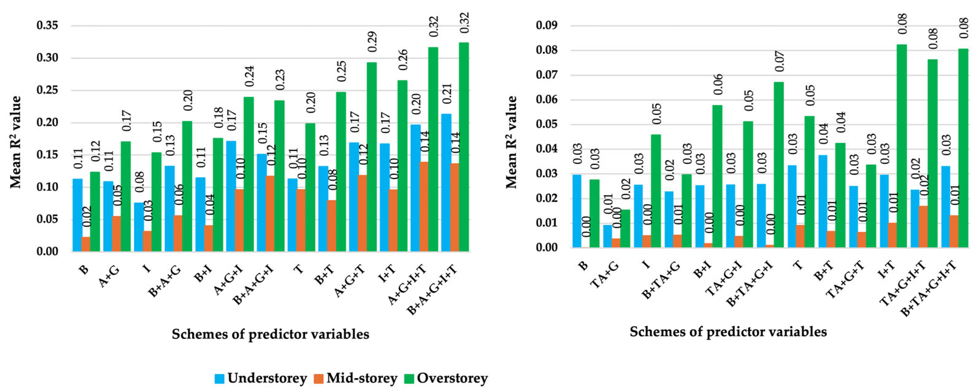
We deployed three density grid layers derived from high-density LiDAR data for the response variables, representing the LiDAR point density in the lower vegetation layer (≥2 m to ≤10 m), a middle vegetation layer (>10 m to ≤30 m), and an upper vegetation layer (>30 m to ≤50 m). The point density values are taken as a proxy for the presence of a forest understorey, mid-storey, and overstorey, respectively. To limit the potential bias caused by the overstorey, this study used the seven highest-intensity returns discretised from high-density full-waveform LiDAR collected from a low flying height (500 m above ground level), achieving a point density of >28 points m⁻². The discretised high-density data ensured that understorey vegetation was captured in sufficient detail.

We tested 13 schemes of different dataset combinations for the predictor variables, combining topographic attributes, texture features, spectral indices, and a geology data layer, as listed below.

We used twelve topographic attributes generated from the DEM, i.e., slope, aspect, catchment area, solar radiation, profile curvature, plan curvature, convergence index, terrain ruggedness index, slope length and steepness (LS) factor, SAGA wetness index, topographic position index, and stream power index. The slope is the angle between the tangent and the horizontal plane at a given point and can be calculated by fitting a plane to the eight neighbouring cells, and the orientation of the cell relative to the north is the aspect [74]. Both were calculated in degrees. A catchment is an upstream area of each cell [75]. The Topographic Wetness Index is an indicator of the potential water content and horizontal depth of the soil [76]. The LS factor, which originated from the slope and length factor (LS), describes the shape of the slope’s vertical profile. It is an indicator of hydrological connectivity and soil erosion and helps in assessing vegetation growth [77]. Profile curvature is the rate of slope change in a downslope direction. In contrast, plan curvature is the curvature of a contour at the central pixel, which is related to an area of erosion potential [78] and determines particle deposition. Both curvatures explain areas of action, aspect, and gradient factors [79]. The convergence index is the average bias of the slope directions of the adjacent cell from the direction of the central cell [75]. The sum change in elevation between a grid cell and its eight neighbouring cells is defined as the terrain ruggedness index [80], and a measure of the erosive power of flowing water is the stream power index [81]. Wetness index is a measure of soil moisture potential [82]. Solar radiation is the result of complex interactions of energy between the atmosphere and Earth’s surface [83].

We derived eight texture features (Appendix A,

Table A1. Selected texture features derived from WorldView-3 and Landsat-8 (OLI) satellite data.

Texture Feature	Description	Equations	References
Contrast	The grey level of the two pixels of the same image varies	${\displaystyle \sum _i}{\displaystyle \sum _j}{(i-j)}^{2}p(i, j)$	[22]
Correlation	Captures how the pairs of pixels are correlated to other pixel pairs	${\displaystyle \frac{\sum _i\sum _{j}ijp\left(i, j\right)-{\mu }_x{\mu }_y}{{\sigma }_x{\sigma }_y}}$	[22]
Dissimilarity	Two samples vary with the number of grey levels	${\displaystyle \sum _i}{\displaystyle \sum _j\left|i-j\right|}.p(i, j)$	[138]
Entropy	Captures the amount of variation in the co-occurrence of the grey level distribution	$-{\displaystyle \sum _i}{\displaystyle \sum _j}p\left(i, j\right)\log (p(i, j))$	[86]
Homogeneity	measures how close the distribution of elements in the GLCM	${\displaystyle \sum _i}{\displaystyle \sum _j}{\displaystyle \frac{1}{1+{(i-j)}^2}} .p(i, j)$	[138]
Mean	Mean value of intensities over the image	${\displaystyle \sum _{i=2}^{2N}}i{p}_{x+y}(i)$	[86]
Angular second moment	a measure of homogeneity of an image/measures the local uniformity of the grey levels	${\displaystyle \sum _i}{\displaystyle \sum _j}{(p\left(i,j\right))}^2$	[86]
Variance	a measure of “roughness”	${\displaystyle \sum _i}{\displaystyle \sum _j}{(i-{\mu }_i)}^{2}p(i, j)$	[22]

Note: Let $p(i, j)$ is the two compared pixels in the image, one with grey level $i$ and the other with a grey level $j. {\mu }_{x, }{ \mu }_y,$ ${\sigma }_x{ \mathrm{and} \sigma }_y$ are the means and standard deviations of $p_x$ and $p_y$. These eight texture features are widely used in the literature and are important variables.

) using the grey-level co-occurrence matrix for each band of multispectral satellite imagery based on their ability to characterise vegetation structure [84,85]. Thus, we derived 128 raster layers of texture features (16 bands × 8) from WorldView-3 of 7.5 m, 64 layers (8 bands × 8) from WorldView-3 of 1.6 m, and 56 layers (7 bands × 8) from Landsat-8 (OLI) 30 m data. Texture identifies objects or regions of interest, and the texture features depend on the grey tone in an image [86], for example, the contrast is the grey level of the two pixels of the same image, and correlation shows the relationship of the pairs of pixels with other pairs of pixels [22] (For more details, see Appendix A, Table A1).

We also extracted fifteen spectral indices from both multispectral satellite imagery (Appendix A,

Table A2. Selected spectral indices derived from WorldView-3 and Landsat-8 (OLI) satellite data.

Spectral Indices	Acronyms	Equations	Reference
Green Atmospherically Resistant Index	GARI	${\displaystyle \frac{NIR - [Green-\gamma \left(Blue-Red\right)]}{NIR+[Green-\gamma \left(Blue-Red\right)]}}$	[139]
Green Normalised Difference Vegetation Index	GNDVI	$(NIR-Green)/(NIR+Green)$	[91]
Infrared Percentage Vegetation Index	IPVI	${\displaystyle \frac{NIR}{NIR+Red}}$	[92]
Modified Non-Linear Index	MNLI	${\displaystyle \frac{\left({NIR}^2-RED\right)\mathrm{\ast }(1+L)}{({NIR}^2-Red+L)}}$	[96]
Modified Soil-Adjusted Vegetation Index	MSAVI	${\displaystyle \frac{2\mathrm{\ast }NIR+\sqrt{({2\mathrm{\ast }NIR+1)}^2-8(NIR-Red)}}{2}}$	[140]
Modified Simple Ratio	MSR	${\displaystyle \frac{\left(\frac{NIR}{Red}\right)-1}{\left(\frac{NIR}{Red}\right)+1}}$	[97]
Non-Linear Index	NLI	${\displaystyle \frac{{NIR}^2-Red}{{NIR}^2+Red}}$	[95]
Normalised Difference Vegetation Index	NDVI	${\displaystyle \frac{(NIR - Red)}{(NIR+Red)}}$	[89]
Renormalised Difference Vegetation Index	RDVI	${\displaystyle \frac{(NIR - Red)}{\sqrt{(NIR+Red)}}}$	[94]
Optimised Soil-Adjusted Vegetation Index	OSAVI	${\displaystyle \frac{(NIR - Red)}{(NIR+Red+0.16)}}$	[93]
Soil-Adjusted Total Vegetation Index	SATVI	${\displaystyle \frac{SWIR1-Red}{SWIR1+Red+L}}\mathrm{\ast }\left(1+L\right)-{\displaystyle \frac{SWIR2}{2}}$	[141,142,143]
Normalised Burn Ratio (not for Landsat (OLI)) data	NBR	${\displaystyle \frac{({NIR}_{858\mathrm{n}\mathrm{m}}-{SWIR}_{2250\mathrm{n}\mathrm{m}})}{({NIR}_{858\mathrm{n}\mathrm{m}}+{SWIR}_{2250\mathrm{n}\mathrm{m}})}}$	[144,145]
Normalised Difference Water Index	NDWI	${\displaystyle \frac{({NIR}_{858\mathrm{n}\mathrm{m}}-{SWIR}_{1640\mathrm{n}\mathrm{m}})}{({NIR}_{858\mathrm{n}\mathrm{m}}+{SWIR}_{1640\mathrm{n}\mathrm{m}})}}$	[145,146]
Surface Water Capacity Index	SWCI	$({\mathrm{S}\mathrm{W}\mathrm{I}\mathrm{R}}_6-{\mathrm{S}\mathrm{W}\mathrm{I}\mathrm{R}}_7)/({\mathrm{S}\mathrm{W}\mathrm{I}\mathrm{R}}_6+{\mathrm{S}\mathrm{W}\mathrm{I}\mathrm{R}}_7)$	[147]
Shortwave Infrared Soil Moisture Index	SIMI	$\sqrt{{\displaystyle \frac{{SWIR}_6^2+{SWIR}_7^2}{2}}}$	[147]

). Vegetation indices (Vis) are crucial for assessing canopy structure and diversity in the landscape. These VIs measure the overall quality of photosynthetic material in vegetation [87]. The normalised difference vegetation index (NDVI) is widely used for the health of vegetation [88], which uses red and near-infrared bands of a satellite image [89], and its values range from +1 to −1. Green normalised difference vegetation index (GNDVI) is an index of the plant’s greenness that uses the green band instead of the red band used in NDVI, and the GNDVI is the most responsive to field-based metrics of vegetation structure and composition [90,91]. The infrared percentage vegetation index (IPVI) is functionally the same as NDVI, and values range from 0 to 1 [92]. Optimised soil-adjusted vegetation index (OSAVI) provides greater soil variation than the soil-adjusted vegetation index using a canopy background factor, L = 0.16, which is a function of vegetation density [93]. Renormalised difference vegetation index (RDVI) highlights healthy vegetation using near-infrared and red bands and is sensitive to the effects of soil and sun viewing angles [94]. Non-linear index (NLI) considers the relationship of surface parameters with many vegetation indices to be non-linear [95], and the modified non-linear index (MNLI) is an advanced form of the NLI, which uses the soil background factor, L = 0.5, from SAVI [96]. Modified simple ratio (MSR) was developed to assess the increased sensitivity to vegetation biophysical parameters, which utilises the simple ratio in the formula [97]. Normalised burn ratio (NBR) is an indicator for determining the severity of fires. Difference normalised burn ratio (dNBR) is calculated from the pre-fire NBR and post-fire NBR to determine the burn severity [98]. Refer to Appendix A, Table A2 for the formula.

Variable selection is mostly not required in non-parametric modelling [99]. However, since this study dealt with a large number of variables, multicollinearity can arise from intercorrelation among independent variables, which impacts the model’s reliability by inflating the variance [100]. It allows the model to overfit the data, which leads to poor predictions, so it is crucial to address multicollinearity in the data before developing the model [100]. We applied a variance inflation factor (VIF), an indicator of multicollinearity [101], to remove the collinear variables using a threshold of 5.0 [102,103,104]. We selected all the variables based on their appropriateness and their established applications in forestry-related studies [105,106]. The following 13 classification schemes were compared for their relative predictive capacity for vegetation density of the three strata:

• Spectral bands (B);
• Topographic attributes and geology (A + G);
• Spectral indices (I);
• Spectral bands, topographic attributes, and geology (B + A + G);
• Spectral bands and spectral indices (B + I);
• Topographic attributes, geology, and spectral indices (A + G + I);
• Spectral bands, topographic attributes, geology, and spectral indices (B + A + G + I);
• Texture features (T);
• Spectral bands and texture features (B + T);
• Topographic attributes, geology, and texture features (A + G + T);
• Spectral indices and texture features (I + T);
• Topographic attributes, geology, spectral indices, and texture features (A + G + I + T);
• Spectral bands, topographic attributes, geology, spectral indices, and texture features (B + A + G + I + T).

In this study, we converted raster datasets into points and then sampled randomly from all the datasets without replacement. All regions of the landscape represented harvested (i.e., not primary forest) sites, rivers, and roads, and no data were removed. Out of the remaining point values, 10,000 point locations were randomly selected [107,108] and then divided into a model training dataset (50%) and an independent validation dataset (50%). From the training dataset, 70% of point locations were randomly drawn for model training and 30% for cross-validation [4,109,110]. To achieve robust and stable results for the models, the cross-validation was repeated 100 times [111,112] for predicting the density of three vegetation layers. The predicted results were finally validated using the independent validation datasets.

2.5. Random Forest Modelling

We used random forest (RF) regression modelling to examine the predictive power of different datasets at different spatial resolutions for VFS. The RF model is capable of efficiently incorporating a large number of continuous and categorical variables [15]. The RF regression algorithm is a bagging technique which employs recursive partitioning to divide the input data into many homogeneous subsets called regression trees (ntree) and then averages the results of all trees. Each tree is independently grown to its maximum size based on bootstrap samples from the training dataset (approximately 67%) without pruning. In each tree, RF selects a random subset of variables (mtry) to determine the split at each node [113]. The ensemble predicts the data that is not in the tree (OOB (out of bag data), approximately 33%), and calculates the difference in the mean square errors between the OOB data and the dataset used to grow the regression trees. The RF algorithm allows us to identify important predictor variables to predict vegetation layers [106]. Variable importance is evaluated based on how much worse the prediction would be if the dataset for that variable were permuted randomly [114], and this can be used in feature selection by determining the importance of each variable in the regression process [115]. In this study, model performance was evaluated using the coefficient of determination (R²) [101,116,117,118]. R² is a measure of success for predicting response variables based on the proportion of variance explained by the regression [119] and is one of the most widely used reliable statistical tool to test the goodness of fit of a model and compare the performance of multiple models [120].

$$R^2=1-{\displaystyle \frac{{\sum }_{i=1}^n{\left({\mathrm{ŷ}}_i-y_i\right)}^2}{{\sum }_{i=1}^n{\left({\mathrm{ŷ}}_i-{\overline{y}}_i\right)}^2}}$$

(1)

where n is the number of observations in the model, $y_i$ is the observed value, ${\mathrm{ŷ}}_i$ denotes the predicted value and $\overline{y}$ is the mean of the observed value.

Because the R² from RF modelling is derived from cross-validation, it provides useful comparisons between models with different numbers of predictors, unlike R² from standard linear models. The RF modelling analysis processes were conducted in the R programming language [121] using libraries randomForest [122], caret, and caTools [123].

We examined the importance of predictor variables to understand the relative importance of those used in this study. We utilised a percentage increase in mean square error (%IncMSE) as a metric for variable importance, which is one of the most widely used scores of importance [124]. This metric is calculated using out-of-bag (OOB) samples in the RF modelling. The higher the %IncMSE value, the more important the variable [125]. We selected the top 20 important predictor variables based on the higher mean square error (MSE) to explore which variables played a significant role in predicting the density of three vegetation layers by comparing the thirteen different data schemes outlined above.

3. Results

3.1. Model Accuracy Assessment

Overall, our results indicate greater predictive accuracy for models based on 30 m compared to 7.5 m or 1.6 m pixel sizes. For 30 m resolution models, the relative performance of the Landsat-8 (OLI) and WorldView-3 datasets differed depending on the predictor variable scheme and vegetation layer considered, but overall, Landsat performed better.

The RF model prediction accuracy for the 30 m pixels of Landsat-8 (OLI) data varied with the inclusion or exclusion of predictor variables, with mean R² (hereafter R²) values ranging from 0.15 to 0.65. The R² values increased with the number of predictor variables in most cases (Figure 3 and Figure 4;

Table 3. Model performance results (mean R²) for the density of understorey, mid-storey, and overstorey using all thirteen data schemes. The mean R² values were averaged from 100 interactions to ensure robustness.

	Landsat 30 m			Resampled WorldView 30 m			Resampled WorldView 7.5 m			WorldView 1.6 m
Dataset Scheme	Understorey	Mid-Storey	Overstorey	Understorey	Mid-Storey	Overstorey	Understorey	Mid-Storey	Overstorey	Understorey	Mid-Storey	Overstorey
Bands only	0.151	0.243	0.439	0.319	0.217	0.396	0.112	0.022	0.123	0.030	0.000	0.028
Topographic attributes only	0.322	0.226	0.390	0.350	0.230	0.438	0.108	0.055	0.170	0.009	0.004	0.015
Indices only	0.165	0.232	0.478	0.294	0.191	0.437	0.075	0.031	0.153	0.026	0.005	0.046
Bands, topographic attributes and geology	0.334	0.359	0.573	0.382	0.279	0.482	0.132	0.056	0.202	0.023	0.005	0.030
Bands and indices	0.203	0.237	0.455	0.354	0.253	0.481	0.114	0.041	0.175	0.026	0.002	0.058
Topographic attributes, geology and indices	0.399	0.367	0.588	0.340	0.329	0.524	0.171	0.096	0.239	0.026	0.005	0.051
Bands, topographic attributes, geology and indices	0.366	0.366	0.580	0.374	0.357	0.547	0.151	0.117	0.234	0.026	0.001	0.067
Textures only	0.254	0.348	0.471	0.370	0.335	0.474	0.113	0.096	0.198	0.034	0.009	0.053
Bands and textures	0.282	0.412	0.560	0.361	0.347	0.482	0.132	0.079	0.247	0.038	0.007	0.042
Topographic attributes, geology and textures	0.389	0.419	0.561	0.279	0.263	0.400	0.169	0.118	0.293	0.025	0.006	0.034
Indices and textures	0.270	0.416	0.560	0.362	0.380	0.505	0.167	0.096	0.265	0.030	0.010	0.082
Topographic attributes, geology, indices and textures	0.436	0.457	0.630	0.352	0.255	0.461	0.196	0.138	0.316	0.024	0.017	0.076
Bands, topographic attributes, geology, indices and textures	0.445	0.449	0.654	0.394	0.296	0.535	0.213	0.136	0.324	0.033	0.013	0.081

). Here, the RF model had the greatest predictive power for the overstorey (R² = 0.65), followed by the mid-storey (R² = 0.46), and the understorey vegetation density had the least predictive power (R² = 0.44).

In this study, for the overstorey vegetation density, the combined scheme of B + A + G + I + T (scheme #13) produced the highest R² (0.65), followed by the scheme A + G + I + T (#12) dataset (R² = 0.63). Spectral indices (I; #3; R² = 0.48) and texture features (T; #8; R² = 0.47) were also useful for predicting the density of the overstorey vegetation of wet eucalypt forests (Figure 3; Table 3). If the textures and spectral indices are combined, this dataset produced a higher model accuracy (I + T; #11; R² = 0.56) than either dataset alone. In the absence of Landsat data, topographic attributes and geology (A + G; #2) had the lowest predictive capacity (R² = 0.39).

In contrast to the overstorey vegetation density, the R² values for the mid-storey did not increase with an increase in the number of predictor variables, with A + G + I + T (#12; R² = 0.46) yielding the highest R², compared to R² = 0.45 for B + A + G + I + T (#13). Again, A+G had substantially lower predictive power (R² = 0.23).

For the understorey vegetation density model, the B + A + G + I + T scheme had equivalent explanatory power to A + G + I + T (both schemes’ R² = 0.44). Overall, the R² values of combined datasets were mostly greater than those of a single dataset. For example, R² values of spectral indices (I; #1; R² = 0.17) and texture features (T; #8; R² = 0.25) were lower compared to the scenarios with combined datasets (I + T; #11; R² = 0.27), although the gain from combining them was less than for the overstorey vegetation density. In contrast to the overstorey and mid-storey, topographic attributes and geology (A + G; #2; R² = 0.32) performed better than several other schemes for predicting the density of the understorey vegetation.

For the models in the schemes with the resampled 30 m WorldView-3 datasets, the R² values ranged from 0.19 to 0.55 (Figure 3; Table 3). Unlike the 30 m Landsat-8 data, the mid-storey vegetation density was the least predicted in most scenarios. The scheme of B + A + G + I (#7) explained the greatest percentage of variance (R² = 0.55) in the overstorey vegetation density, followed by that of B + A + G + I + T (#13; R² = 0.53), and the model using spectral indices (I) had the lowest explanatory value (R² = 0.19). For the mid-storey vegetation density, the combined spectral indices and texture features (I + T; #11) explained the highest percentage of variation (R² = 0.38), whereas the B + A + G + I + T explained the highest variance (R² = 0.39) in the understory vegetation density, closely followed by B + A + G (#4; R² = 0.38).

Comparing the schemes of the 30 m Landsat-8 (OLI) with the resampled 30 m WorldView-3 dataset, the WorldView-3 imagery could predict the understorey vegetation density better than the mid-storey vegetation density. In contrast, the schemes with the Landsat-8 (OLI) dataset could better predict the mid-storey vegetation density than the understorey vegetation density. Overall, at a 30 m scale, the Landsat-8 data had better predictive power than the WorldView-3 imagery for all three vegetation layers.

The predictive capacity of models was found to be lower for smaller pixel sizes compared to the 30 m resolution models described above. For 7.5 m pixel sizes with WorldView-3 imagery, combining the resampled VNIR bands and original SWIR bands, the predicted R² values ranged from 0.02 to 0.32 (Figure 4; Table 3). The overstorey vegetation density had the highest predictive power (R² = 0.32), followed by the understorey vegetation density (R² = 0.21), and the mid-storey vegetation density (R² = 0.14) had the least predictive capacity. Combinations of two or more datasets provided better predictions than any of the individual datasets in this case.

For the 1.6 m pixel size of the original VNIR eight band WorldView-3 imagery and LiDAR-derived topographic attributes, the overall result demonstrated poor predictive power, with R² values ranging from 0.0 to 0.08 (Figure 4; Table 3). The overstorey vegetation density had a stronger predictive capacity than the mid-storey and understorey vegetation layers. Thus, we inferred that the WorldView-3 imagery with a pixel size of 1.6 m and its combinations were inappropriate for predicting the vertical layers of wet eucalypt forests.

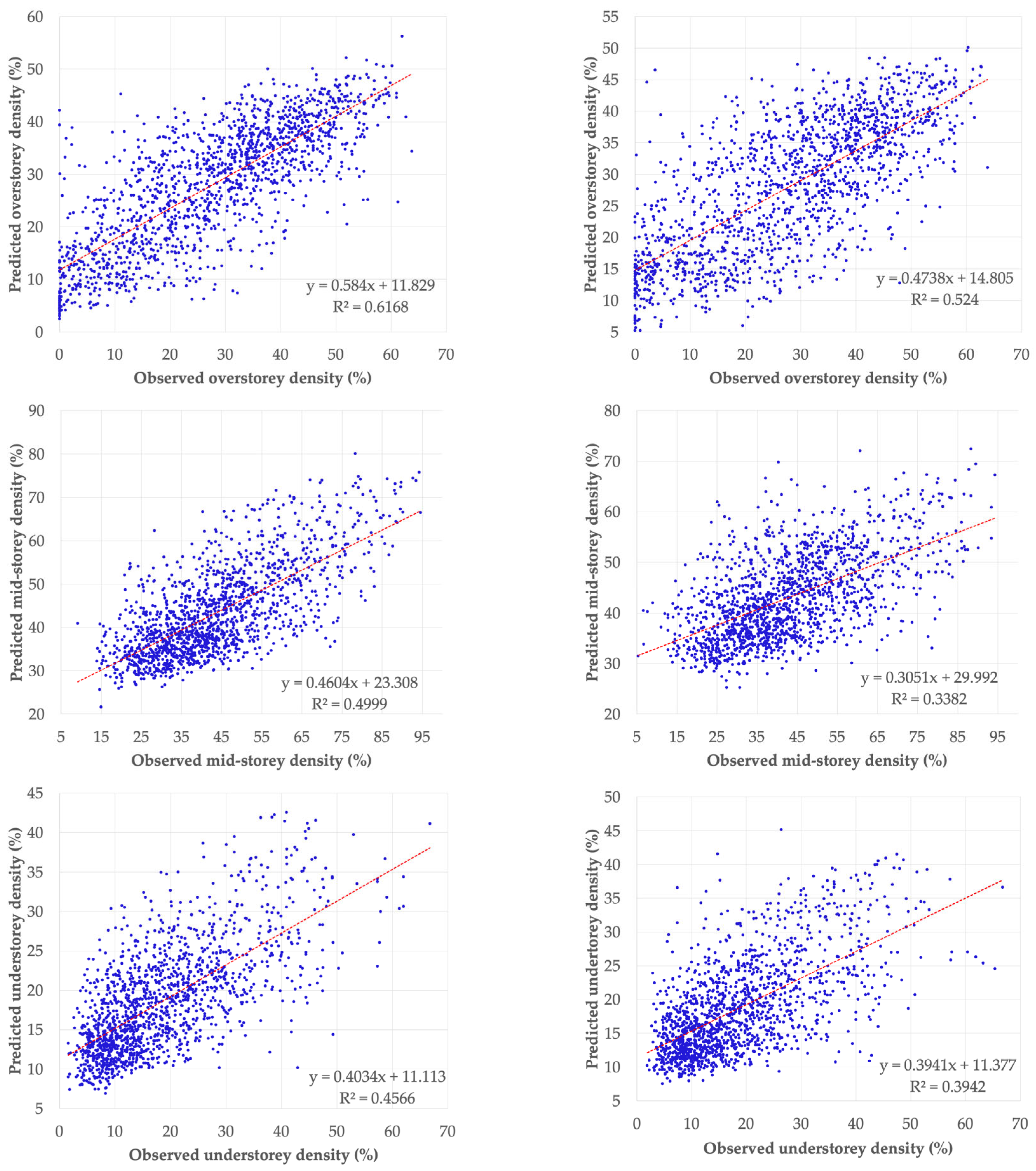
3.2. Model Validation

We evaluated prediction model accuracies using the validation dataset (30%) as shown in the scatter plots (Figure 5) and then an independent validation dataset (Figure 6) to confirm the robustness of the acquired models to Tasmanian wet forests beyond our study landscape. The scatter plots compare the observed and predicted canopy densities at the overstorey, mid-storey, and understorey layers. The overstorey vegetation density for both Landsat (OLI) and the resampled WorldView of 30 m clearly showed a strong positive linear relationship, where most of the observed density values increased with the increase in the predicted density values, with R² values of 61.68% and 52.4%, respectively. The correlation between observed and predicted was lower for the mid-storey with R² values of 0.50 and 0.34, and the understorey with R² values of 45.66% and 39.42% for Landsat and WorldView data, respectively.

In this study, we first calculated the mean R² value using 100 iterations and 30% of the validation dataset. We then used an independent validation dataset and calculated the R² value. The mean R² value calculated from 30% of the validation dataset was subtracted from the R² value calculated using the independent validation dataset to ensure the robustness of the predictions. The differences between the predicted and validated R² values (validated–predicted) were small (<5.67%) across all models. We considered two criteria for robustness: (1) the model with higher prediction and validation accuracies, and (2) the smaller the difference between validated and predicted R² values, the more robust the model. This study indicates that the developed models are robust and, thus, appropriate for transferring to other areas in the forest landscape.

3.3. Importance of Individual Predictor Variables

We present the top 20 important individual predictor variables using Landsat-8 (OLI) and WorldView-3 datasets at three pixel resolutions (Figure 7 for 30 m, and Figure A1 for 1.6 m and 7.5 m), combined with topographic attributes, spectral indices, and texture features.

For predicting the overstorey vegetation density with the Landsat-8 (OLI) dataset, the Normalised Difference Water Index (NDWI) (%IncMSE = 104.0) was the most important variable, followed by geology (%IncMSE = 96.3) (Figure 7). Using the resampled 30 m WorldView dataset, Surface Water Capacity Index (SWCI) (%IncMSE = 66.4) ranked as the most important predictor variable, followed by Normalised Burn Ratio (NBR) (%IncMSE = 41.5) (Figure 7). Saga Wetness Index, GNDVI, and LS factor were important predictors for these models. Other variables for the overstorey vegetation density, for example, SWI, CI, SIMI, and SPI using the Landsat-8 (OLI) dataset, and GNDVI, RDVI, TRI, and SIMI using the 30 m WorldView dataset produced lower variable importance scores.

For the mid-storey vegetation density, a variance of band#4 (%IncMSE = 90.2) was the most important predictor, followed by NDWI (%IncMSE = 65.5) and then geology (%IncMSE = 45.0) using the Landsat-8 (OLI) dataset. Solar radiation (%IncMSE = 65.9) was the most important predictor variable, followed by SATVI (%IncMSE = 28.4) and then SWCI (%IncMSE = 27.9) using the Worldview 30 m dataset.

Similarly, for the understorey vegetation density, geology (%IncMSE = 58.0) was the most important predictor, followed by the LS factor (%IncMSE = 40.6) and solar radiation (%IncMSE = 36.7) using the Landsat-8 (OLI) dataset. In contrast, SWCI (%IncMSE = 55.5) was the most important predictor variable followed by GARI (%IncMSE = 46.1) and then band#1 (%IncMSE = 29.1) using the WorldView 30 m dataset.

For the WorldView dataset at 7.5 m resolution, band#16 (SWIR band#8) (%IncMSE = 46.7) and WorldView band#1 (%IncMSE = 34.7) produced the highest variable importance scores for the overstorey and understorey vegetation layers, respectively (Figure A1). The 1.6 m resolution WorldView dataset provided the mean of band#1 (%IncMSE = 27.3) for the understorey, geology (%IncMSE = 15.2) for the overstorey, and again geology (%IncMSE = 8.9) for the mid-storey vegetation density as the most important variables (Figure A1).

4. Discussion

This study demonstrates that, in the absence of expensive high-resolution LiDAR data, the density of three vegetation strata can be predicted with reasonable accuracy from a combination of affordable multispectral satellite imagery, topographic attributes derived from DEMs, and a geology spatial layer. We assessed the influence of spatial resolution and satellite platform and found that 30 m resolution data outperformed 7.5 m and 1.6 m pixel sizes, and 30 m Landsat-8 (OLI) data outperformed 30 m resampled WorldView-3 data. We found the greatest predictive capacity from a combination of topographic attributes derived from a DEM, texture features and spectral indices from satellite imagery, and a geology spatial layer.

Our study defined vertical forest structure (VFS) as the understorey, mid-storey, and overstorey vegetation layers widely recognised by botanists for this ecosystem, excluding the ground and herb layer vegetation, which is likely to be poorly captured by airborne LiDAR data at this resolution. Prior research conducted by White [126] using the same high-resolution LiDAR dataset as our study compared LiDAR data to 40 field plots (20 m radius) that were located using a stratified random approach to capture the variation in forest structure in the region. White [126] found a strong correlation between LiDAR-derived point density values and understorey and mid-storey vegetation within the field plots he sampled. White [126] also checked for the potential blocking effect of the overstorey canopy on the understorey data and reported that the canopy had a minimal impact on the density of the understorey data. Our study, therefore, builds on these earlier findings and uses point density as a proxy for understorey presence over a 5 km × 5 km region. Much of our study landscape is an example of wilderness without roads and it is impractical for conducting ground-based vegetation surveys, highlighting the immense value of remote sensing data in remote regions.

Comparing all the thirteen schemes, the spatial resolution of the freely available 30 m Landsat-8 (OLI) dataset and its combinations with the topographic attributes derived from the resampled LiDAR and geology data produced the best result (R² = 0.65) for the overstorey vegetation density followed by the mid-storey (R² = 0.46) and then the understorey vegetation density (R² = 0.44) (Figure 3). Models based on Landsat-8 (OLI) data combinations were consistently better than those found on the WorldView-3 dataset. The highest performing WorldView-3 model was at 30 m resampled resolution, combined with topographic attributes and geology (R² = 0.55 for the overstorey vegetation density; Figure 3).

Across datasets, predictive accuracy was generally increased with an increasing number of predictor variables. The models that included pixel-values of spectral bands, indices and texture features from the multispectral datasets, topographic attributes derived from a DEM created from the resampled operational LiDAR data, and ancillary geology vector data produced the best overall prediction accuracy (R² = 0.65 for the overstorey vegetation density). The combination of three data sources provided higher model performance than the combinations with the satellite spectral indices and texture features in isolation, or the operational LiDAR DEM topographic attributes and geology. Although the relationships between image texture metrics and forest structure attributes can be used to characterise complex forest structures and enhance vegetation properties, the uses of vegetation indices, particularly in the case of closed canopies, are difficult and challenging [127].

In this study, the spatial resolution of the 1.6 m WorldView-3 dataset was not considered appropriate for modelling vertical forest structure, as the R² values ranged from 0.0 to 0.08 (Figure 4). The results demonstrate that the resolution of remote sensing datasets was inversely proportional to the prediction accuracy for three vegetation density layers. The poor performance of the 1.6 m resolution WorldView-3 dataset for all three vegetation layers considered is likely related to the mismatch between the high spatial resolution of the satellite pixels and the spatial scale of the response variables. Since the LiDAR points were divided into three vegetation layers and the ground, the 1.6 m spatial resolution dataset might have produced lower prediction accuracy due to a lack of LiDAR points within the 1.6 m pixels. The spatial uncertainties in the datasets may have a greater effect on small pixels than on large pixels; for example, the canopy may be more homogeneous at coarser resolution and produce a better prediction, which can be a topic of future research.

Despite focusing on a different forest type, our results were in broad accordance with those of Latifi et al. [128], who used RF modelling of Landsat-5 Thematic Mapper (TM) imagery with LiDAR data to predict forest structural attributes. They also reported that accuracy was increased with the number of predictor variables and emphasised the utility of topographic variables derived from LiDAR data over the multispectral satellite data.

The optimal pixel size observed here (30 m) may be related to the canopy tree crown size for our overstorey layer, with Azaele et al. [129] and Cohen and Spies [50] finding that the spatial resolution of the dataset should match the object to be predicted. Cohen and Spies [50] postulated that the pixel size of Landsat TM data is roughly equivalent in size to the tree crowns. In contrast, a large tree may appear in many pixels if pixel sizes are smaller, for example, 7.5 m or 1.6 m, as tested in this study, and this consequently produced lower model accuracy. Munsamy et al. [130] tested resolutions from 1 m to up to 9 m and found that coarser spatial resolutions produced the best results for predicting dominant and mean tree height in mature stands in South Africa. Therefore, a study requiring information on individual tree canopies may be expected to require a larger pixel size than studies requiring information on individual branches or smaller plants in lower canopy layers. However, further research is required to explore why the 30 m pixel size performed best for understorey and mid-storey vegetation, where individual plants have much smaller canopies than 30 m in diameter. Likewise, we are unable to explain why model predictive capacity was higher for the overstorey layer. We hypothesise that the 30 m pixel size was better for creating indirect predictors, and some of the key predictors were at a coarser scale, regardless of the vegetation layers.

It is important to note that we could not compare direct canopy density estimates for operational LiDAR with those of high-resolution LiDAR, which would be worthy of future research. Operational LiDAR was unavailable for much of the study area, and it was deemed inappropriate to compare direct density estimates from the down-sampled high-resolution LiDAR since this subset would have included the same points as for the comparison dataset, artificially inflating their explanatory value. Potapov et al. [131] used airborne LiDAR data as a proxy for field surveys and the reference for model calibration and validation. Mäyrä et al. [132] also suggested high-resolution airborne data for training for landscape-level species detection utilising spaceborne data. Therefore, this study focused on combining multispectral satellite data and topographic attributes derived from the resampled LiDAR data.

The Landsat-8 (OLI) dataset produced the best overall results for each vegetation layer. However, the 30 m Landsat-8 (OLI) and the 30 m resampled WorldView-3 datasets produced contrasting outcomes for relative abilities to predict the mid-storey and understory vegetation densities. We are unable to explain the difference in performance between these two sensor platforms. The original (7.5 m and 1.6 m resolution) and resampled (30 m resolution) WorldView-3 data could predict understory vegetation density better than mid-storey vegetation density, whereas Landsat-8 (OLI) data predicted mid-storey vegetation density better than understory vegetation density. This study recommends that when high-density LiDAR data are unavailable, using freely available Landsat-8 imagery combined with geology and DEM-derivatives (topographic attributes), texture measures and vegetation indices can be adequate for forest managers and planners to assess the VFS of wet eucalypt forests, to contribute to sustainable management, planning, and monitoring of forests.

In general, the predicted accuracy of the models compared favourably with those of previous research in other forest systems and confirmed the validity of the approach of this study. A study conducted by Zald et al. [24] advocated that prediction accuracy depended on structural variable type using derivatives from LiDAR and Landsat data and presented R² ranging from 0.0 to 0.77, with the highest value for structural variables, including live trees and the lowest for downed wood. They found that metrics derived from Landsat data improved the prediction accuracies of all the structural variables, although those improvements were less than the inclusion of LiDAR data. Similarly, Wallner et al. [133] stratified forest plots based on forest types and showed R² values ranging from 0.37 to 0.63 for modelling stand structural attributes using RapidEye data, particularly R² values of 0.4 for stand density. Kayitakire et al. [22] reported the model prediction with an R² value of 0.38 for stand density. Therefore, this research can act as a benchmark for including a broad range of explanatory variables; however, further research is required to translate this approach to other types of forest ecosystems and satellite imagery (e.g., Sentinel-2) with different topography and understorey conditions.

Our study validated the predicted accuracies with promising goodness of fit statistics (differences between the predicted and validated R² values were <5.67%), suggesting our best models could be applied to larger geographical areas and indicating the capability of LiDAR-derived metrics to predict vertical structural variables with reasonable accuracy. Bolton et al. [23] achieved negative model bias (−1.2 to −2.1%) and validated their research in other study systems to examine transferability. They suggested that the structural variability in the new systems might not have been captured in the training plots used in the model development, and the bias varied from −3.9% to −8.0%. Therefore, further research would be required to test the robustness and transferability of our models to other wet forest landscapes, with due consideration given to the forest age, structure, management history (our models excluded previously harvested and wildfire-impacted forests), underlying geology, and rainfall.

The best predictor for overstorey density derived from the Landsat-8 (OLI) dataset with topographic attributes, indices, and texture features (scheme #13) was the Normalised Difference Water Index (NDWI) (%IncMSE = 104.0). The second-ranked variable was geology (%IncMSE = 96.3) for the overstorey vegetation density (Figure 7). For mid-storey vegetation density, the variance of band#4 (one of the texture features) ranked first, followed by NDWI. Similarly, SWCI (%IncMSE = 55.5) ranked first, followed by GARI (%IncMSE = 46.1) for the understorey vegetation density.

Li et al. [103] reported that texture features from Landsat-8 showed a significant correlation with the aboveground biomass, and the variance of Landsat band#4 performed best in predicting biomass. Using spectral indices and textural variables in combination with Landsat bands, Halperin et al. [134] compared the Landsat-8 (OLI) dataset with RapidEye for canopy cover estimation in Zambia. They found Landsat-8 (OLI) consistently performed better than RapidEye and soil data improved the model accuracy. They inferred that vegetation indices were the most important variables. Nasiri et al. [135] evaluated predictor variables and reported that vegetation indices were dominant predictors in most of the models. Forest health, foliage density, chlorophyll content, water stress, and tree biomass influenced forest canopy cover, resulting in the determination of important variables [134].

The topographic attributes derived from a DEM could be deployed in combination with Landsat-8 (OLI) datasets, as their contributions were each high in the models, demonstrating the advantage of combining the multispectral data rather than relying solely on topographic attributes derived from a DEM [125]. The freely available Landsat dataset could be used for modelling and mapping larger geographical areas and is easily adopted by forestry professionals, bushfire managers, and ecologists who require stand-level details of VFS.

5. Conclusions

The aim of this study was to predict the density of three vegetation layers in a wet eucalypt forest in Tasmania, Australia, based on multispectral satellite imagery and topographic attributes derived from a DEM generated from the simulated operational LiDAR data as well as a geology spatial layer. We applied a random forest machine learning approach to model the density of the forest understorey, mid-storey, and overstorey based on a range of spectral indices (15) and texture features (8) per spectral band derived from multispectral satellite data and 12 terrain attributes derived from LiDAR data. We tested the impact of spatial resolution by applying the random forest algorithm at three resolutions: 1.6 m, 7.5 m, and 30 m, corresponding to the visible bands of Worldview-3, the SWIR bands of Worldview-3, and Landsat 8 OLI, respectively.

The fusion of the derivatives from the 30 m Landsat-8 (OLI) satellite imagery and DEM derivatives (topographic attributes) and geology produced the best overall results (R² = 0.65 for the overstorey layer). The classification schemes utilising Landsat-8 (OLI) datasets outperformed models based on high-resolution WorldView-3 imagery.

Spectral indices and texture features were useful for predicting the overstorey vegetation density of wet eucalypt forests. If the texture features and spectral indices were combined with topographic attributes, the combined dataset produced higher model accuracy than either dataset alone.

The analysed output demonstrated that the resampled 30 m WorldView-3 data showed better model performance than at original pixel sizes of 7.5 m and 1.6 m. The schemes with WorldView-3 datasets with a pixel size of 1.6 m were inappropriate for predicting the density of three vegetation layers of a wet eucalypt forest. Landsat-8 outperformed WorldView-3 imagery for all three pixel sizes and all three vegetation layers.

The results showed an increase in model accuracies with an increasing number of predictor variables in most schemes, illustrating the merit of combining topographic attributes, geology, texture features, and spectral indices.

The differences between the predicted and validated accuracies were less than 5.7% for all models. This indicates that the developed models are robust and could be transferred to similar forests outside the focal research landscape. Our findings also show that texture features and spectral indices are important variables that can be used for vertical forest structure modelling.

Further work would be required to validate this approach and extend the results to different forest types and age classes, since this study was confined to mature wet eucalypt forests. It would be valuable to test this approach on the topographic attributes derived from the spaceborne Global Ecosystem Dynamics Investigation (GEDI) LiDAR data (footprints averaging 25 m in diameter) [136] combined with the Landsat-8 (OLI) and Sentinel-2 imagery for predicting and mapping VFS over larger geographic areas. Our study suggests that freely available spatial data, including Landsat, DEM, and geology, could be used as predictor variables, enabling forest managers and planners to adopt the approach presented in this study even where LiDAR data are unavailable. If information is required on forest species composition as well as vertical structure, our previous research has demonstrated the utility of combining LiDAR with hyperspectral data to identify the canopies of overstorey and mid-storey trees [137].

References

1. Zhou, X.; Li, C. Mapping the vertical forest structure in a large subtropical region using airborne LiDAR data. Ecol. Indic. 2023, 154, 110731. [Google Scholar] [CrossRef]
2. Blondeel, H.; Landuyt, D.; Vangansbeke, P.; De Frenne, P.; Verheyen, K.; Perring, M.P. The need for an understory decision support system for temperate deciduous forest management. For. Ecol. Manag. 2021, 480, 118634. [Google Scholar] [CrossRef]
3. Dubayah, R.; Blair, J.B.; Goetz, S.; Fatoyinbo, L.; Hansen, M.; Healey, S.; Hofton, M.; Hurtt, G.; Kellner, J.; Luthcke, S.; et al. The Global Ecosystem Dynamics Investigation: High-resolution laser ranging of the Earth’s forests and topography. Sci. Remote Sens. 2020, 1, 100002. [Google Scholar] [CrossRef]
4. Jarron, L.R.; Coops, N.C.; MacKenzie, W.H.; Tompalski, P.; Dykstra, P. Detection of sub-canopy forest structure using airborne LiDAR. Remote Sens. Environ. 2020, 244, 111770. [Google Scholar] [CrossRef]
5. Peng, X.; Zhao, A.; Chen, Y.; Chen, Q.; Liu, H.; Wang, J.; Li, H. Comparison of Modeling Algorithms for Forest Canopy Structures Based on UAV-LiDAR: A Case Study in Tropical China. Forests 2020, 11, 1324. [Google Scholar] [CrossRef]
6. Wei, L.; Gosselin, F.; Rao, X.; Lin, Y.; Wang, J.; Jian, S.; Ren, H. Overstory and niche attributes drive understory biomass production in three types of subtropical plantations. For. Ecol. Manag. 2021, 482, 118894. [Google Scholar] [CrossRef]
7. Rutten, G.; Ensslin, A.; Hemp, A.; Fischer, M. Vertical and horizontal vegetation structure across natural and modified habitat types at Mount Kilimanjaro. PLoS ONE 2015, 10, e0138822. [Google Scholar] [CrossRef]
8. Dash, J.P.; Watt, M.S.; Bhandari, S.; Watt, P. Characterising forest structure using combinations of airborne laser scanning data, RapidEye satellite imagery and environmental variables. Forestry 2016, 89, 159–169. [Google Scholar] [CrossRef]
9. Wilkes, P.; Jones, S.D.; Suarez, L.; Haywood, A.; Mellor, A.; Woodgate, W.; Soto-Berelov, M.; Skidmore, A.K.; McMahon, S. Using discrete-return airborne laser scanning to quantify number of canopy strata across diverse forest types. Methods Ecol. Evol. 2016, 7, 700–712. [Google Scholar] [CrossRef]
10. Furlaud, J.M.; Prior, L.D.; Williamson, G.J.; Bowman, D.M.J.S. Fire risk and severity decline with stand development in Tasmanian giant Eucalyptus forest. For. Ecol. Manag. 2021, 502, 119724. [Google Scholar] [CrossRef]
11. Lee, Y.-S.; Lee, S.; Jung, H.-S. Mapping Forest Vertical Structure in Gong-ju, Korea Using Sentinel-2 Satellite Images and Artificial Neural Networks. Appl. Sci. 2020, 10, 1666. [Google Scholar] [CrossRef]
12. Taneja, R.; Wallace, L.; Hillman, S.; Reinke, K.; Hilton, J.; Jones, S.; Hally, B. Up-Scaling Fuel Hazard Metrics Derived from Terrestrial Laser Scanning Using a Machine Learning Model. Remote Sens. 2023, 15, 1273. [Google Scholar] [CrossRef]
13. Viedma, O.; Moreno, J.M. Impact of LiDAR pulse density on forest fuels metrics derived using LadderFuelsR. Ecol. Inform. 2025, 88, 103135. [Google Scholar] [CrossRef]
14. Silva, I.; Rocha, R.; López-Baucells, A.; Farneda, F.Z.; Meyer, C.F.J. Effects of Forest Fragmentation on the Vertical Stratification of Neotropical Bats. Diversity 2020, 12, 67. [Google Scholar] [CrossRef]
15. Wilkes, P.; Jones, S.; Suarez, L.; Mellor, A.; Woodgate, W.; Soto-Berelov, M.; Haywood, A.; Skidmore, A. Mapping forest canopy height across large areas by upscaling ALS estimates with freely available satellite data. Remote Sens. 2015, 7, 12563. [Google Scholar] [CrossRef]
16. Terryn, L.; Calders, K.; Bartholomeus, H.; Bartolo, R.E.; Brede, B.; D’Hont, B.; Disney, M.; Herold, M.; Lau, A.; Shenkin, A.; et al. Quantifying tropical forest structure through terrestrial and UAV laser scanning fusion in Australian rainforests. Remote Sens. Environ. 2022, 271, 112912. [Google Scholar] [CrossRef]
17. Cardenas-Martinez, A.; Pascual, A.; Guisado-Pintado, E.; Rodriguez-Galiano, V. Using airborne LiDAR and enhanced-geolocated GEDI metrics to map structural traits over a Mediterranean forest. Sci. Remote Sens. 2025, 11, 100195. [Google Scholar] [CrossRef]
18. Linderman, M.; Liu, J.; Qi, J.; An, L.; Ouyang, Z.; Yang, J.; Tan, Y. Using artificial neural networks to map the spatial distribution of understorey bamboo from remote sensing data. Int. J. Remote Sens. 2004, 25, 1685–1700. [Google Scholar] [CrossRef]
19. Culbert, P.; Radeloff, V.; Flather, C.; Kellndorfer, J.; Rittenhouse, C.; Pidgeon, A. The influence of vertical and horizontal habitat structure on nationwide patterns of avian biodiversity. Ornithology 2013, 130, 656–665. [Google Scholar] [CrossRef]
20. Masek, J.G.; Hayes, D.J.; Joseph Hughes, M.; Healey, S.P.; Turner, D.P. The role of remote sensing in process-scaling studies of managed forest ecosystems. For. Ecol. Manag. 2015, 355, 109–123. [Google Scholar] [CrossRef]
21. Ozdemir, I.; Karnieli, A. Predicting forest structural parameters using the image texture derived from WorldView-2 multispectral imagery in a dryland forest, Israel. Int. J. Appl. Earth Obs. Geoinf. 2011, 13, 701–710. [Google Scholar] [CrossRef]
22. Kayitakire, F.; Hamel, C.; Defourny, P. Retrieving forest structure variables based on image texture analysis and IKONOS-2 imagery. Remote Sens. Environ. 2006, 102, 390–401. [Google Scholar] [CrossRef]
23. Bolton, D.K.; White, J.C.; Wulder, M.A.; Coops, N.C.; Hermosilla, T.; Yuan, X. Updating stand-level forest inventories using airborne laser scanning and Landsat time series data. Int. J. Appl. Earth Obs. Geoinf. 2018, 66, 174–183. [Google Scholar] [CrossRef]
24. Zald, H.S.J.; Wulder, M.A.; White, J.C.; Hilker, T.; Hermosilla, T.; Hobart, G.W.; Coops, N.C. Integrating Landsat pixel composites and change metrics with LiDAR plots to predictively map forest structure and aboveground biomass in Saskatchewan, Canada. Remote Sens. Environ. 2016, 176, 188–201. [Google Scholar] [CrossRef]
25. Zald, H.S.J.; Ohmann, J.L.; Roberts, H.M.; Gregory, M.J.; Henderson, E.B.; McGaughey, R.J.; Braaten, J. Influence of LiDAR, Landsat imagery, disturbance history, plot location accuracy, and plot size on accuracy of imputation maps of forest composition and structure. Remote Sens. Environ. 2014, 143, 26–38. [Google Scholar] [CrossRef]
26. Gebreslasie, M.T.; Ahmed, F.B.; van Aardt, J.A.N. Predicting forest structural attributes using ancillary data and ASTER satellite data. Int. J. Appl. Earth Obs. Geoinf. 2010, 12, S23–S26. [Google Scholar] [CrossRef]
27. Venier, L.A.; Swystun, T.; Mazerolle, M.J.; Kreutzweiser, D.P.; Wainio-Keizer, K.L.; McIlwrick, K.A.; Woods, M.E.; Wang, X. Modelling vegetation understory cover using LiDAR metrics. PLoS ONE 2019, 14, e0220096. [Google Scholar] [CrossRef]
28. Kamal, M.; Phinn, S.; Johansen, K. Characterizing the spatial structure of mangrove features for optimizing image-based mangrove mapping. Remote Sens. 2014, 6, 984. [Google Scholar] [CrossRef]
29. Kunin, W.E.; Harte, J.; He, F.; Hui, C.; Jobe, R.T.; Ostling, A.; Polce, C.; Šizling, A.; Smith, A.B.; Smith, K.; et al. Upscaling biodiversity: Estimating the species–area relationship from small samples. Ecol. Monogr. 2018, 88, 170–187. [Google Scholar] [CrossRef]
30. Zhang, N. Scale issues in ecology: Upscaling. Acta Ecol. Sin. 2007, 27, 4252–4266. [Google Scholar]
31. Yang, X.; Qiu, S.; Zhu, Z.; Rittenhouse, C.; Riordan, D.; Cullerton, M. Mapping understory plant communities in deciduous forests from Sentinel-2 time series. Remote Sens. Environ. 2023, 293, 113601. [Google Scholar] [CrossRef]
32. Luo, Y.; Qi, S.; Liao, K.; Zhang, S.; Hu, B.; Tian, Y. Mapping the Forest Height by Fusion of ICESat-2 and Multi-Source Remote Sensing Imagery and Topographic Information: A Case Study in Jiangxi Province, China. Forests 2023, 14, 454. [Google Scholar] [CrossRef]
33. Ni, M.; Wu, Q.; Li, G.; Li, D. Remote Sensing Technology for Observing Tree Mortality and Its Influences on Carbon–Water Dynamics. Forests 2025, 16, 194. [Google Scholar] [CrossRef]
34. Miura, N.; Jones, S.D. Characterizing forest ecological structure using pulse types and heights of airborne laser scanning. Remote Sens. Environ. 2010, 114, 1069–1076. [Google Scholar] [CrossRef]
35. Moudrý, V.; Cord, A.F.; Gábor, L.; Laurin, G.V.; Barták, V.; Gdulová, K.; Malavasi, M.; Rocchini, D.; Stereńczak, K.; Prošek, J.; et al. Vegetation structure derived from airborne laser scanning to assess species distribution and habitat suitability: The way forward. Divers. Distrib. 2022, 29, 39–50. [Google Scholar] [CrossRef]
36. Guo, Q.; Su, Y.; Hu, T.; Guan, H.; Jin, S.; Zhang, J.; Zhao, X.; Xu, K.; Wei, D.; Kelly, M.; et al. Lidar Boosts 3D Ecological Observations and Modelings: A Review and Perspective. IEEE Geosci. Remote Sens. Mag. 2021, 9, 232–257. [Google Scholar] [CrossRef]
37. Atkins, J.W.; Costanza, J.; Dahlin, K.M.; Dannenberg, M.P.; Elmore, A.J.; Fitzpatrick, M.C.; Hakkenberg, C.R.; Hardiman, B.S.; Kamoske, A.; LaRue, E.A.; et al. Scale dependency of lidar-derived forest structural diversity. Methods Ecol. Evol. 2023, 14, 708–723. [Google Scholar] [CrossRef]
38. Kim, J.; Popescu, S.C.; Lopez, R.R.; Wu, X.B.; Silvy, N.J. Vegetation mapping of No Name Key, Florida using lidar and multispectral remote sensing. Int. J. Remote Sens. 2020, 41, 9469–9506. [Google Scholar] [CrossRef]
39. Bigdeli, B.; Amini Amirkolaee, H.; Pahlavani, P. DTM extraction under forest canopy using LiDAR data and a modified invasive weed optimization algorithm. Remote Sens. Environ. 2018, 216, 289–300. [Google Scholar] [CrossRef]
40. Bolton, D.K.; Coops, N.C.; Wulder, M.A. Characterizing residual structure and forest recovery following high-severity fire in the western boreal of Canada using Landsat time-series and airborne lidar data. Remote Sens. Environ. 2015, 163, 48–60. [Google Scholar] [CrossRef]
41. Hagar, J.C.; Yost, A.; Haggerty, P.K. Incorporating LiDAR metrics into a structure-based habitat model for a canopy-dwelling species. Remote Sens. Environ. 2020, 236, 111499. [Google Scholar] [CrossRef]
42. Lesak, A.A.; Radeloff, V.C.; Hawbaker, T.J.; Pidgeon, A.M.; Gobakken, T.; Contrucci, K. Modeling forest songbird species richness using LiDAR-derived measures of forest structure. Remote Sens. Environ. 2011, 115, 2823–2835. [Google Scholar] [CrossRef]
43. Carrasco, L.; Giam, X.; Papeş, M.; Sheldon, K.S. Metrics of Lidar-Derived 3D Vegetation Structure Reveal Contrasting Effects of Horizontal and Vertical Forest Heterogeneity on Bird Species Richness. Remote Sens. 2019, 11, 743. [Google Scholar] [CrossRef]
44. Wang, D.; Wan, B.; Liu, J.; Su, Y.; Guo, Q.; Qiu, P.; Wu, X. Estimating aboveground biomass of the mangrove forests on northeast Hainan Island in China using an upscaling method from field plots, UAV-LiDAR data and Sentinel-2 imagery. Int. J. Appl. Earth Obs. Geoinf. 2020, 85, 101986. [Google Scholar] [CrossRef]
45. Dupuis, C.; Lejeune, P.; Michez, A.; Fayolle, A. How Can Remote Sensing Help Monitor Tropical Moist Forest Degradation?—A Systematic Review. Remote Sens. 2020, 12, 1087. [Google Scholar] [CrossRef]
46. LaRue, E.A.; Wagner, F.W.; Fei, S.; Atkins, J.W.; Fahey, R.T.; Gough, C.M.; Hardiman, B.S. Compatibility of Aerial and Terrestrial LiDAR for Quantifying Forest Structural Diversity. Remote Sens. 2020, 12, 1407. [Google Scholar] [CrossRef]
47. Hudak, A.T.; Crookston, N.L.; Evans, J.S.; Falkowski, M.J.; Smith, A.M.S.; Gessler, P.E.; Morgan, P. Regression modeling and mapping of coniferous forest basal area and tree density from discrete-return lidar and multispectral satellite data. Can. J. Remote Sens. 2006, 32, 126–138. [Google Scholar] [CrossRef]
48. Sun, X.; Li, G.; Wu, Q.; Ruan, J.; Li, D.; Lu, D. Mapping Forest Carbon Stock Distribution in a Subtropical Region with the Integration of Airborne Lidar and Sentinel-2 Data. Remote Sens. 2024, 16, 3847. [Google Scholar] [CrossRef]
49. Arroyo, L.A.; Johansen, K.; Armston, J.; Phinn, S. Integration of LiDAR and QuickBird imagery for mapping riparian biophysical parameters and land cover types in Australian tropical savannas. For. Ecol. Manag. 2010, 259, 598–606. [Google Scholar] [CrossRef]
50. Cohen, W.B.; Spies, T.A. Estimating structural attributes of Douglas-fir/western hemlock forest stands from landsat and SPOT imagery. Remote Sens. Environ. 1992, 41, 1–17. [Google Scholar] [CrossRef]
51. Muscarella, R.; Kolyaie, S.; Morton, D.C.; Zimmerman, J.K.; Uriarte, M. Effects of topography on tropical forest structure depend on climate context. J. Ecol. 2020, 108, 145–159. [Google Scholar] [CrossRef]
52. Gracia, M.; Montané, F.; Piqué, J.; Retana, J. Overstory structure and topographic gradients determining diversity and abundance of understory shrub species in temperate forests in central Pyrenees (NE Spain). For. Ecol. Manag. 2007, 242, 391–397. [Google Scholar] [CrossRef]
53. Odom, R.; Henry McNab, W. Using Digital Terrain Modeling to Predict Ecological Types in the Balsam Mountains of Western North Carolina; RN-SRS008; Department of Agriculture, Forest Service, Southern Research Station: Asheville, NC, USA, 2000; p. 13. [Google Scholar]
54. Conrad, O.; Bechtel, B.; Bock, M.; Dietrich, H.; Fischer, E.; Gerlitz, L.; Wehberg, J.; Wichmann, V.; Böhner, J. System for Automated Geoscientific Analyses (SAGA) v. 2.1.4. Geosci. Model Dev. 2015, 8, 1991–2007. [Google Scholar] [CrossRef]
55. Mikita, T.; Klimánek, M.; Miloš, C. Evaluation of airborne laser scanning data for tree parameters and terrain modelling in forest environment. Acta Univ. Agric. Silvic. Mendel. Brun. 2013, LXI, 1339–1347. [Google Scholar] [CrossRef]
56. Yun, Z.; Zheng, G.; Geng, Q.; Monika Moskal, L.; Wu, B.; Gong, P. Dynamic stratification for vertical forest structure using aerial laser scanning over multiple spatial scales. Int. J. Appl. Earth Obs. Geoinf. 2022, 114, 103040. [Google Scholar] [CrossRef]
57. TERN. Warra Tall Eucalypt SuperSite. Available online: https://www.tern.org.au/tern-ecosystem-processes/warra-tall-eucalypt-supersite/ (accessed on 15 July 2017).
58. Bureau of Meteorology. Climate Statistics for Australian Locations (2004–2017); Bureau of Meteorology: Canberra, Australia, 2017. [Google Scholar]
59. Hickey, J.E.; Su, W.; Rowe, P.; Brown, M.J.; Edwards, L. Fire history of the tall wet eucalypt forests of the Warra ecological research site, Tamania. Aust. For. 1999, 62, 66–71. [Google Scholar] [CrossRef]
60. Baker, S.C.; Garandel, M.; Deltombe, M.; Neyland, M.G. Factors influencing initial vascular plant seedling composition following either aggregated retention harvesting and regeneration burning or burning of unharvested forest. For. Ecol. Manag. 2013, 306, 192–201. [Google Scholar] [CrossRef]
61. Neyland, M.G. Vegetation of the Warra silvicultural systems trial. Tasforests 2001, 13, 183–192. [Google Scholar]
62. Mineral Resources Tasmania. Digital Geological Atlas 1:25,000 Scale Series. Available online: http://www.mrt.tas.gov.au/products/geoscience_maps/digital_geological_atlas_125_000_scale_series (accessed on 30 January 2019).
63. Assmann, J.J.; Moeslund, J.; Treier, U.; Normand, S. EcoDes-DK15: High-resolution ecological descriptors of vegetation and terrain derived from Denmark’s national airborne laser scanning data set. Earth Syst. Sci. Data 2022, 14, 823–844. [Google Scholar] [CrossRef]
64. Meijer, C.; Grootes, M.; Koma, Z.; Dzigan, Y.; Gonçalves, R.; Andela, B.; Oord, G.; Ranguelova, E.; Renaud, N.; Kissling, W.D. Laserchicken—A tool for distributed feature calculation from massive LiDAR point cloud datasets. SoftwareX 2020, 12, 100626. [Google Scholar] [CrossRef]
65. Ferro, J.C.; Warner, T. Scale and texture in digital image classification. Photogramm. Eng. Remote Sens. 2002, 68, 51–63. [Google Scholar]
66. Neyland, M.G.; Jarman, S.J. Early impacts of harvesting and burning disturbances on vegetation communities in the Warra silvicultural systems trial, Tasmania, Australia. Aust. J. Bot. 2011, 59, 701–712. [Google Scholar] [CrossRef]
67. Wardlaw, T.J.; Grove, S.J.; Hingston, A.B.; Balmer, J.M.; Forster, L.G.; Musk, R.A.; Read, S.M. Responses of flora and fauna in wet eucalypt production forest to the intensity of disturbance in the surrounding landscape. For. Ecol. Manag. 2018, 409, 694–706. [Google Scholar] [CrossRef]
68. Roussel, J.-R.; Auty, D.; Coops, N.C.; Tompalski, P.; Goodbody, T.R.H.; Meador, A.S.; Bourdon, J.-F.; de Boissieu, F.; Achim, A. lidR: An R package for analysis of Airborne Laser Scanning (ALS) data. Remote Sens. Environ. 2020, 251, 112061. [Google Scholar] [CrossRef]
69. Shi, Y.; Wang, T.; Skidmore, A.K.; Holzwarth, S.; Heiden, U.; Heurich, M. Mapping individual silver fir trees using hyperspectral and LiDAR data in a Central European mixed forest. Int. J. Appl. Earth Obs. Geoinf. 2021, 98, 102311. [Google Scholar] [CrossRef]
70. Ehlers, S.; Saarela, S.; Lindgren, N.; Lindberg, E.; Nyström, M.; Persson, H.; Olsson, H.; Ståhl, G. Assessing Error Correlations in Remote Sensing-Based Estimates of Forest Attributes for Improved Composite Estimation. Remote Sens. 2018, 10, 667. [Google Scholar] [CrossRef]
71. Kuester, M. Radiometric Use of WorldView-3 Imagery-Technical Note; DigitalGlobe: Longmont, CO, USA, 2016; pp. 1–12. [Google Scholar]
72. Flood, N. Continuity of reflectance data between Landsat-7 ETM+ and Landsat-8 OLI, for both top-of-atmosphere and surface reflectance: A study in the Australian landscape. Remote Sens. 2014, 6, 7952. [Google Scholar] [CrossRef]
73. Thuillier, G.; Hersé, M.; Labs, D.; Foujols, T.; Peetermans, W.; Gillotay, D.; Simon, P.C.; Mandel, H. The solar spectral irradiance from 200 to 2400 nm as measured by the SOLSPEC Spectrometer from the Atlas and Eureca Missions. Sol. Phys. 2003, 214, 1–22. [Google Scholar] [CrossRef]
74. Travis, M.R.; Elsner, G.H.; Iverson, W.D.; Jonnson, C.G. VIEWIT: Computation of Seen Areas, Slope, and Aspect for Landuse Planning; USDA Forest Service, General Technical Report, PSW-1111975, 70; Pacific Southwest Forest and Range Exp. Stn.: Berkeley, CA, USA; Forest Service, U.S. Department of Agriculture: Berkeley, CA, USA, 1975; p. 67. [Google Scholar]
75. Kiss, R. Determination of drainage network in digital elevation models, utilities and limitations. J. Hung. Geomath. 2004, 2, 16–29. [Google Scholar]
76. Beven, K.J.; Kirkby, M.J. A physically based, variable contributing area model of basin hydrology/Un modèle à base physique de zone d’appel variable de l’hydrologie du bassin versant. Hydrol. Sci. Bull. 1979, 24, 43–69. [Google Scholar] [CrossRef]
77. Zhou, F.; Ma, G.; Xie, C.; Zhang, Y.; Xiao, Z. Application of Compound Terrain Factor LSW in Vegetation Cover Evaluation. Appl. Sci. 2023, 13, 11806. [Google Scholar] [CrossRef]
78. Wilson, M.F.J.; O’Connell, B.; Brown, C.; Guinan, J.C.; Grehan, A.J. Multiscale terrain analysis of multibeam bathymetry data for habitat mapping on the continental slope. Mar. Geod. 2007, 30, 3–35. [Google Scholar] [CrossRef]
79. Shary, P. Land surface in gravity points classification by a complete system of curvatures. Math. Geol. 1995, 27, 373–390. [Google Scholar] [CrossRef]
80. Riley, S.; Degloria, S.; Elliot, S.D. A terrain ruggedness index that quantifies topographic heterogeneity. Int. J. Sci. 1999, 5, 23–27. [Google Scholar]
81. Jacoby, B.; Peterson, E.; Dogwiler, T. Identifying the Stream Erosion Potential of Cave Levels in Carter Cave State Resort Park, Kentucky, USA. J. Geogr. Inf. Syst. 2011, 3, 323–333. [Google Scholar] [CrossRef]
82. Gessler, P.E.; Moore, I.D.; McKenzie, N.J.; Ryan, P.J. Soil-landscape modelling and spatial prediction of soil attributes. Int. J. Geogr. Inf. Syst. 1995, 9, 421–432. [Google Scholar] [CrossRef]
83. Lukovic, J.; Bajat, B.; Kilibarda, M.; Filipovic, D. High resolution grid of potential incoming solar radiation for Serbia. Therm. Sci. 2015, 19, 427–435. [Google Scholar] [CrossRef]
84. Dobrowski, S.Z.; Safford, H.D.; Cheng, Y.B.; Ustin, S.L. Mapping mountain vegetation using species distribution modeling, image-based texture analysis, and object-based classification. Appl. Veg. Sci. 2008, 11, 499–508. [Google Scholar] [CrossRef]
85. Ge, S.; Carruthers, R.; Gong, P.; Herrera, A. Texture analysis for mapping Tamarix parviflora using aerial photographs along the Cache Creek, California. Environ. Monit. Assess. 2006, 114, 65–83. [Google Scholar] [CrossRef]
86. Haralick, R.M.; Shanmugam, K.; Dinstein, I. Textural features for image classification. IEEE Trans. Syst. Man Cybern. 1973, SMC-3, 610–621. [Google Scholar] [CrossRef]
87. Darra, N.; Espejo-Garcia, B.; Psiroukis, V.; Psomiadis, E.; Fountas, S. Spectral bands vs. vegetation indices: An AutoML approach for processing tomato yield predictions based on Sentinel-2 imagery. Smart Agric. Technol. 2025, 10, 100805. [Google Scholar] [CrossRef]
88. Anand, S.; Kumar, H.; Kumar, P.; Kumar, M. Analyzing landscape changes and their relationship with land surface temperature and vegetation indices using remote sensing and AI techniques. Geosci. Lett. 2025, 12, 7. [Google Scholar] [CrossRef]
89. Rouse, J.; Haas, R.; Schell, J.; Deering, D. Monitoring vegetation systems in the great plains with ERTS (Earth Resources Technology Satellite). In Proceedings of the Third ERTS Symposium, Goddard Space Flight Center, Greenbelt, MD, USA, 10–14 December 1973; pp. 309–317. [Google Scholar]
90. Taddeo, S.; Dronova, I.; Depsky, N. Spectral vegetation indices of wetland greenness: Responses to vegetation structure, composition, and spatial distribution. Remote Sens. Environ. 2019, 234, 111467. [Google Scholar] [CrossRef]
91. Gitelson, A.A.; Merzlyak, M.N. Remote sensing of chlorophyll concentration in higher plant leaves. Adv. Space Res. 1998, 22, 689–692. [Google Scholar] [CrossRef]
92. Crippen, R.E. Calculating the vegetation index faster. Remote Sens. Environ. 1990, 34, 71–73. [Google Scholar] [CrossRef]
93. Rondeaux, G.; Steven, M.; Baret, F. Optimization of soil-adjusted vegetation indices. Remote Sens. Environ. 1996, 55, 95–107. [Google Scholar] [CrossRef]
94. Roujean, J.-L.; Breon, F.-M. Estimating PAR absorbed by vegetation from bidirectional reflectance measurements. Remote Sens. Environ. 1995, 51, 375–384. [Google Scholar] [CrossRef]
95. Goel, N.S.; Qin, W. Influences of canopy architecture on relationships between various vegetation indices and LAI and Fpar: A computer simulation. Remote Sens. Rev. 1994, 10, 309–347. [Google Scholar] [CrossRef]
96. Yang, Z.; Willis, P.; Mueller, R. Impact of band-ratio enhanced AWIFS image on crop classification accuracy. In Proceedings of the Pecora 17—The Future of Land Imaging…Going Operational, Denver, CO, USA, 18–20 November 2008; p. 11. [Google Scholar]
97. Chen, J.M. Evaluation of vegetation indices and a modified simple ratio for boreal applications. Can. J. Remote Sens. 1996, 22, 229–242. [Google Scholar] [CrossRef]
98. Ghazali, N.N.; Saraf, N.M.; Rasam, A.R.A.; Othman, A.N.; Salleh, S.A.; Saad, N.M. Forest Fire Severity Level Using dNBR Spectral Index. Rev. Int. Geomat. 2025, 34, 89–101. [Google Scholar] [CrossRef]
99. Iqbal, I.A.; Musk, R.A.; Osborn, J.; Stone, C.; Lucieer, A. A comparison of area-based forest attributes derived from airborne laser scanner, small-format and medium-format digital aerial photography. Int. J. Appl. Earth Obs. Geoinf. 2019, 76, 231–241. [Google Scholar] [CrossRef]
100. Lukman, A.F.; Mohammed, S.; Olaluwoye, O.; Farghali, R.A. Handling Multicollinearity and Outliers in Logistic Regression Using the Robust Kibria–Lukman Estimator. Axioms 2024, 14, 19. [Google Scholar] [CrossRef]
101. Shrestha, N. Detecting Multicollinearity in Regression Analysis. Am. J. Appl. Math. Stat. 2020, 8, 39–42. [Google Scholar] [CrossRef]
102. Imdadullah, M.; Aslam, M.; Altaf, S. mctest: An R package for detection of collinearity among regressors. R J. 2016, 8, 495–505. [Google Scholar] [CrossRef]
103. Li, Y.; Li, M.; Li, C.; Liu, Z. Forest aboveground biomass estimation using Landsat 8 and Sentinel-1A data with machine learning algorithms. Sci. Rep. 2020, 10, 9952. [Google Scholar] [CrossRef]
104. Abonazel, M.R. A New Biased Estimation Class to Combat the Multicollinearity in Regression Models: Modified Two--Parameter Liu Estimator. Comput. J. Math. Stat. Sci. 2025, 4, 316–347. [Google Scholar] [CrossRef]
105. Jaskierniak, D.; Lane, P.N.J.; Robinson, A.; Lucieer, A. Extracting LiDAR indices to characterise multilayered forest structure using mixture distribution functions. Remote Sens. Environ. 2011, 115, 573–585. [Google Scholar] [CrossRef]
106. Martinuzzi, S.; Vierling, L.A.; Gould, W.A.; Falkowski, M.J.; Evans, J.S.; Hudak, A.T.; Vierling, K.T. Mapping snags and understory shrubs for a LiDAR-based assessment of wildlife habitat suitability. Remote Sens. Environ. 2009, 113, 2533–2546. [Google Scholar] [CrossRef]
107. Campbell, M.J.; Dennison, P.E.; Hudak, A.T.; Parham, L.M.; Butler, B.W. Quantifying understory vegetation density using small-footprint airborne LiDAR. Remote Sens. Environ. 2018, 215, 330–342. [Google Scholar] [CrossRef]
108. Criminisi, A.; Shotton, J.; Konukoglu, E. Decision Forests for Classification, Regression, Density Estimation, Manifold Learning and Semi-Supervised Learning; Microsoft Research Technical Report TR-2011-114; Microsoft: Cambridge, UK, 2011; p. 151. [Google Scholar]
109. Kemppinen, J.; Niittynen, P.; Riihimäki, H.; Luoto, M. Modelling soil moisture in a high-latitude landscape using LiDAR and soil data. Earth Surf. Process. Landf. 2018, 43, 1019–1031. [Google Scholar] [CrossRef]
110. Wang, M.; Zheng, Y.; Huang, C.; Meng, R.; Pang, Y.; Jia, W.; Zhou, J.; Huang, Z.; Fang, L.; Zhao, F. Assessing Landsat-8 and Sentinel-2 spectral-temporal features for mapping tree species of northern plantation forests in Heilongjiang Province, China. For. Ecosyst. 2022, 9, 100032. [Google Scholar] [CrossRef]
111. van Galen, L.G.; Jordan, G.J.; Musk, R.A.; Beeton, N.J.; Wardlaw, T.J.; Baker, S.C. Quantifying floristic and structural forest maturity: An attribute-based method for wet eucalypt forests. J. Appl. Ecol. 2018, 55, 1668–1681. [Google Scholar] [CrossRef]
112. Astola, H.; Häme, T.; Sirro, L.; Molinier, M.; Kilpi, J. Comparison of Sentinel-2 and Landsat 8 imagery for forest variable prediction in boreal region. Remote Sens. Environ. 2019, 223, 257–273. [Google Scholar] [CrossRef]
113. Breiman, L. Random forests. Mach. Learn. 2001, 45, 5–32. [Google Scholar] [CrossRef]
114. Prasad, A.M.; Iverson, L.R.; Liaw, A. Newer classification and regression tree techniques: Bagging and random forests for ecological prediction. Ecosystems 2006, 9, 181–199. [Google Scholar] [CrossRef]
115. Freeman, E.A.; Moisen, G.G.; Coulston, J.W.; Wilson, B.T. Random forests and stochastic gradient boosting for predicting tree canopy cover: Comparing tuning processes and model performance. Can. J. For. Res. 2015, 46, 323–339. [Google Scholar] [CrossRef]
116. Valbuena, R.; Hernando, A.; Manzanera, J.A.; Görgens, E.B.; Almeida, D.R.A.; Silva, C.A.; García-Abril, A. Evaluating observed versus predicted forest biomass: R-squared, index of agreement or maximal information coefficient? Eur. J. Remote Sens. 2019, 52, 345–358. [Google Scholar] [CrossRef]
117. Mohammed, K.; Kpienbaareh, D.; Wang, J.; Goldblum, D.; Luginaah, I.; Lupafya, E.; Dakishoni, L. Synthesizing Local Capacities, Multi-Source Remote Sensing and Meta-Learning to Optimize Forest Carbon Assessment in Data-Poor Regions. Remote Sens. 2025, 17, 289. [Google Scholar] [CrossRef]
118. Ling, Q.; Chen, Y.; Feng, Z.; Pei, H.; Wang, C.; Yin, Z.; Qiu, Z. Monitoring Canopy Height in the Hainan Tropical Rainforest Using Machine Learning and Multi-Modal Data Fusion. Remote Sens. 2025, 17, 966. [Google Scholar] [CrossRef]
119. Nagelkerke, N.J.D. A Note on a General Definition of the Coefficient of Determination. Biometrika 1991, 78, 691–692. [Google Scholar] [CrossRef]
120. Sapra, R.L. Using R2 with caution. Curr. Med. Res. Pract. 2014, 4, 130–134. [Google Scholar] [CrossRef]
121. R Core Team. R: A Language and Environment for Statistical Computing, Version 3.4.1; R Foundation for Statistical Computing: Vienna, Austria, 2017. Available online: https://www.r-project.org/ (accessed on 20 July 2018).
122. Liaw, A.; Wiener, M. Classification and Regression by randomForest. R News 2002, 2, 18–22. [Google Scholar]
123. Tuszynski, J. Tools: Moving Window Statistics, GIF, Base64, ROC AUC, etc. R Package Version 1.18.0. Available online: https://cran.r-project.org/package=caTools (accessed on 15 March 2020).
124. Genuer, R.; Poggi, J.-M.; Tuleau-Malot, C. VSURF: An R package for variable selection using random forests. R J. 2015, 7, 19–33. [Google Scholar] [CrossRef]
125. Yadav, B.K.V.; Lucieer, A.; Jordan, G.J.; Baker, S.C. Using topographic attributes to predict the density of vegetation layers in a wet eucalypt forest. Aust. For. 2022, 85, 25–37. [Google Scholar] [CrossRef]
126. White, R.J. Searching for Rainforest Understorey in Wet Eucalyptus Forest. Bachelor’s Thesis, School of Biological Sciences, University of Tasmania, Hobart, Australia, 2017. [Google Scholar] [CrossRef]
127. Dube, T.; Mutanga, O. Investigating the robustness of the new Landsat-8 Operational Land Imager derived texture metrics in estimating plantation forest aboveground biomass in resource constrained areas. ISPRS J. Photogramm. Remote Sens. 2015, 108, 12–32. [Google Scholar] [CrossRef]
128. Latifi, H.; Nothdurft, A.; Straub, C.; Koch, B. Modelling stratified forest attributes using optical/LiDAR features in a central European landscape. Int. J. Digit. Earth 2012, 5, 106–132. [Google Scholar] [CrossRef]
129. Azaele, S.; Cornell, S.J.; Kunin, W.E. Downscaling species occupancy from coarse spatial scales. Ecol. Appl. 2012, 22, 1004–1014. [Google Scholar] [CrossRef] [PubMed]
130. Munsamy, R.; Gebreslasie, M.; Peerbhay, K.; Ismail, R. Modelling the effect of terrain variability in even-aged Eucalyptus species using LiDAR-derived DTM variables. S. Afr. J. Geomat. 2020, 9, 118–135. [Google Scholar] [CrossRef]
131. Potapov, P.; Li, X.; Hernandez-Serna, A.; Tyukavina, A.; Hansen, M.C.; Kommareddy, A.; Pickens, A.; Turubanova, S.; Tang, H.; Silva, C.E.; et al. Mapping global forest canopy height through integration of GEDI and Landsat data. Remote Sens. Environ. 2021, 253, 112165. [Google Scholar] [CrossRef]
132. Mäyrä, J.; Keski-Saari, S.; Kivinen, S.; Tanhuanpää, T.; Hurskainen, P.; Kullberg, P.; Poikolainen, L.; Viinikka, A.; Tuominen, S.; Kumpula, T.; et al. Tree species classification from airborne hyperspectral and LiDAR data using 3D convolutional neural networks. Remote Sens. Environ. 2021, 256, 112322. [Google Scholar] [CrossRef]
133. Wallner, A.; Elatawneh, A.; Knoke, T.; Schneider, T. Estimation of forest structural information using RapidEye satellite data. For. Int. J. For. Res. 2014, 88, 96–107. [Google Scholar] [CrossRef]
134. Halperin, J.; LeMay, V.; Coops, N.; Verchot, L.; Marshall, P.; Lochhead, K. Canopy cover estimation in miombo woodlands of Zambia: Comparison of Landsat 8 OLI versus RapidEye imagery using parametric, nonparametric, and semiparametric methods. Remote Sens. Environ. 2016, 179, 170–182. [Google Scholar] [CrossRef]
135. Nasiri, V.; Darvishsefat, A.A.; Arefi, H.; Griess, V.C.; Sadeghi, S.M.M.; Borz, S.A. Modeling Forest Canopy Cover: A Synergistic Use of Sentinel-2, Aerial Photogrammetry Data, and Machine Learning. Remote Sens. 2022, 14, 1453. [Google Scholar] [CrossRef]
136. Chen, L.; Ren, C.; Zhang, B.; Wang, Z.; Liu, M.; Man, W.; Liu, J. Improved estimation of forest stand volume by the integration of GEDI LiDAR data and multi-sensor imagery in the Changbai Mountains Mixed forests Ecoregion (CMMFE), northeast China. Int. J. Appl. Earth Obs. Geoinf. 2021, 100, 102326. [Google Scholar] [CrossRef]
137. Yadav, B.K.V.; Lucieer, A.; Baker, S.C.; Jordan, G.J. Tree crown segmentation and species classification in a wet eucalypt forest from airborne hyperspectral and LiDAR data. Int. J. Remote Sens. 2021, 42, 7952–7977. [Google Scholar] [CrossRef]
138. Soh, L.-K.; Tsatsoulis, C. Texture analysis of SAR sea ice imagery using gray level co-occurrence matrices. IEEE Trans. Geosci. Remote Sens. 1999, 37, 780–795. [Google Scholar] [CrossRef]
139. Gitelson, A.A.; Kaufman, Y.J.; Merzlyak, M.N. Use of a green channel in remote sensing of global vegetation from EOS-MODIS. Remote Sens. Environ. 1996, 58, 289–298. [Google Scholar] [CrossRef]
140. Qi, J.; Chehbouni, A.; Huete, A.R.; Kerr, Y.H.; Sorooshian, S. A modified soil adjusted vegetation index. Remote Sens. Environ. 1994, 48, 119–126. [Google Scholar] [CrossRef]
141. Marsett, R.C.; Qi, J.; Heilman, P.; Biedenbender, S.H.; Carolyn Watson, M.; Amer, S.; Weltz, M.; Goodrich, D.; Marsett, R. Remote sensing for grassland management in the arid southwest. Rangel. Ecol. Manag. 2006, 59, 530–540. [Google Scholar] [CrossRef]
142. Hagen, S.C.; Heilman, P.; Marsett, R.; Torbick, N.; Salas, W.; van Ravensway, J.; Qi, J. Mapping total vegetation cover across western rangelands with moderate-resolution imaging spectroradiometer data. Rangel. Ecol. Manag. 2012, 65, 456–467. [Google Scholar] [CrossRef]
143. Torbick, N.; Ledoux, L.; Salas, W.; Zhao, M. Regional mapping of plantation extent using multisensor imagery. Remote Sens. 2016, 8, 236. [Google Scholar] [CrossRef]
144. Key, C.H.; Benson, N.C. Landscape assessment: Ground measure of severity, the composite burn index; and remote sensing of severity, the normalized burn ratio. In FIREMON: Fire Effects Monitoring and Inventory System, RMRS-GTR-164 ed.; Lutes, D.C., Keane, R.E., Caratti, J.F., Key, C.H., Benson, N.C., Sutherland, S., Gangi, L.J., Eds.; USDA Forest Service, Rocky Mountain Research Station: Ogden, UT, USA, 2006; p. 56. [Google Scholar]
145. Ji, L.; Zhang, L.; Wylie, B.; Rover, J. On the terminology of the spectral vegetation index (NIR − SWIR)/(NIR + SWIR). Int. J. Remote Sens. 2011, 32, 6901–6909. [Google Scholar] [CrossRef]
146. Chen, D.; Huang, J.; Jackson, T.J. Vegetation water content estimation for corn and soybeans using spectral indices derived from MODIS near- and short-wave infrared bands. Remote Sens. Environ. 2005, 98, 225–236. [Google Scholar] [CrossRef]
147. Zhang, N.; Hong, Y.; Qin, Q.; Zhu, L. Evaluation of the visible and shortwave infrared drought index in China. Int. J. Disaster Risk Sci. 2013, 4, 68–76. [Google Scholar] [CrossRef]
Figure 1. Geographical location map of the study site. The digital elevation model with the hill shade shows a 5 km by 5 km study area. The map in the bottom-left corner shows the state of Tasmania, with the study site in red. Two sample photos on the right side show the structure of the forest in the study site.
Remotesensing 17 01733 g001
Figure 2. Workflow for assessing the robustness of multispectral satellite imagery with LiDAR topographic attributes and a geology data layer to predict vertical structure in a wet eucalypt forest.
Remotesensing 17 01733 g002
Figure 3. Predicted mean R2 of the density of three vegetation layers from the 13 schemes of predictor variables derived from the 30 m Landsat-8 (OLI) (left) and the 30 m resampled WorldView-3 satellite data (right) and simulated operational LiDAR data. Here, a scheme means a group of predictor variables used for RF modelling. Spectral bands = B, spectral indices = I, texture features = T, topographic attributes = A, geology vector data = G.
Remotesensing 17 01733 g003
Figure 4. Mean R2 of predicted density of three vegetation layers from the 13 schemes of predictor variables derived from the 7.5 m (left) and 1.6 m spatial resolutions (right) of WorldView-3 satellite imagery and the simulated operational LiDAR data. Spectral bands = B, spectral indices = I, texture features = T, topographic attributes = A, geology vector data = G.
Remotesensing 17 01733 g004
Figure 5. Scatter plots of predicted values against observed (true) values (blue) using Landsat-8 (OLI) satellite data (left) and the resampled 30 m WorldView-3 data (right) with topographic attributes and geology data. The Linear line of best fit (red dotted line) is shown on each plot. The equation of a line of best fit and the coefficient of determination (R2) for each relationship are shown.
Remotesensing 17 01733 g005
Figure 6. Accuracy differences (validated-predicted density values for three vegetation layers) of thirteen schemes using the 30 m Landsat-8 satellite data (left) and the 30 m WorldView-3 data (right) along with topographic attributes and geology data. Positive and negative values indicate the robustness of the models.
Remotesensing 17 01733 g006
Figure 7. Importance of the top 20 predictor variables using Landsat-8 (OLI) bands (left) and the resampled bands of WorldView 30 m (right) combined with topographic attributes, spectral indices, and texture features.
Remotesensing 17 01733 g007