Article

Spatiotemporal Dynamics and Driving Mechanisms of Soil Conservation Services (SCS) in Zhejiang Province, China: Insights from InVEST Modeling and Machine Learning

1
School of Computer Science and Technology, Beijing Jiaotong University, No. 8212, Zhixing Building, No. 3 Shangyuancun, Haidian District, Beijing 100044, China
2
School of Geography and Environment, Jiangxi Normal University, 99 Ziyang Road, Nanchang 330022, China
3
College of Life Sciences, Huzhou University, 759 East 2nd Ring Road, Wuxing District, Huzhou 313000, China
4
Graduate School of Integrated Sciences for Global Society, Kyushu University, Motooka 744, Nishi-ku, Fukuoka 8190395, Japan
*
Author to whom correspondence should be addressed.
Remote Sens. 2025, 17(16), 2865; https://doi.org/10.3390/rs17162865 (registering DOI)
Submission received: 6 June 2025 / Revised: 9 August 2025 / Accepted: 14 August 2025 / Published: 17 August 2025
(This article belongs to the Special Issue GeoAI and EO Big Data Driven Advances in Earth Environmental Science)

Abstract

Zhejiang Province, as a key ecological region in southeastern China, plays a vital role in ensuring regional ecological security and sustainable development through its soil conservation services (SCS). Based on remote sensing data, this study employed the InVEST model to evaluate the characteristics of SCS in Zhejiang from 2001 to 2020. Long-term trends were identified using Sen’s Slope and the Mann–Kendall test, spatial autocorrelation was assessed through Moran’s I, the contributions of driving factors were quantified using XGBoost combined with SHAP, and spatial heterogeneity was further explored using Geographically Weighted Regression (GWR). The results indicate that: (1) from 2001 to 2020, SCS exhibited a fluctuating trend of “decline followed by recovery,” with significantly higher values in the western mountainous areas than in the eastern coastal and plain regions; approximately 58% of the area remained stable, while 40% experienced degradation; (2) Spatial autocorrelation analysis showed that areas with strong SCS were concentrated in the western mountains, while low-value areas were mainly distributed in the eastern coastal and urban regions; (3) natural factors contributed the most, followed by climatic and human activity factors; and (4) the GWR model outperformed the OLS model in revealing the spatial variation in the effects of natural and anthropogenic drivers. These findings provide valuable scientific references and decision-making support for ecological conservation, watershed management, and sustainable land use in Zhejiang Province.

1. Introduction

Ecosystem services encompass a wide range of direct and indirect contributions provided by natural systems that support human life and development [1,2,3]. They form the basis for human well-being, regional sustainability, and long-term economic development [4]. Among these services, soil conservation services (SCS) play a vital role in maintaining land productivity, reducing soil erosion, and regulating hydrological processes [5,6]. However, accelerating industrialization and urbanization have imposed unprecedented pressure on ecosystems worldwide, resulting in the degradation of ecological functions, depletion of resources, and growing environmental risks [7,8,9]. Around one million species are at risk of extinction, and annual losses in crop production due to pollinator decline are estimated at USD 577 billion [10]. If current trends in ecosystem degradation continue, the global economy could suffer cumulative GDP losses of up to USD 9.87 trillion by 2050, as a result of declining ecosystem services under a business-as-usual scenario [11]. In light of these alarming developments, there is an urgent need to understand the spatiotemporal dynamics of SCS and identify the driving forces behind their changes to support sustainable land use and ecological management [12,13].
Accurately assessing SCS requires an evaluation framework that can simultaneously capture both biophysical processes and human–environment interactions [14]. Over the years, researchers have developed a variety of methodological systems, including empirical statistics, geostatistical approaches, process-based modeling, and integrated analyses that utilize remote sensing data and geographic information systems technologies [15]. Among them, the Revised Universal Soil Loss Equation (RUSLE), known for its simplicity and clear parameters, has been widely used for estimating soil erosion at regional scales. The InVEST model, which provides process-based simulation within the ecosystem service assessment framework, has been extensively applied in ecological compensation, watershed management, and land use planning [16]. In recent years, the research focus has gradually shifted from quantifying service magnitude to evaluating supply–demand relationships and simulating future scenarios [17]. For instance, Jian et al. [18] proposed a soil conservation service supply–demand ratio based on the InVEST and PLUS models, and systematically assessed the spatial patterns and multi-scenario changes on the Loess Plateau. In terms of mechanism analysis, Fan et al. [19] employed a modified wind erosion equation and partial derivative method to quantify the relative contributions of climate change and human activities to changes in sand fixation services, revealing significant spatial heterogeneity and key thresholds [20]. However, most existing studies remain focused on result-based assessments and lack in-depth analysis of nonlinear interactions among driving mechanisms, particularly in coastal regions characterized by strong spatial heterogeneity [21].
As China’s southeastern coastal ecological security barrier, Zhejiang Province lies within the Yangtze River Delta economic region, one of the most economically dynamic areas nationally and simultaneously one of the most ecologically stressed [22]. With a forest coverage rate among the highest in the country, SCS plays an irreplaceable role in maintaining regional ecological security, reducing soil erosion, and safeguarding downstream water resources. However, rapid industrialization and urbanization in recent years have significantly altered land-use patterns, particularly through the encroachment of agricultural land and forests, posing severe challenges to ecosystem service functions. Existing studies have largely focused on water resource management and carbon stock assessments in Zhejiang, while comprehensive evaluations of soil retention service functions—especially those integrating spatial–temporal dynamics with driver analysis—remain scarce. Therefore, investigating the spatial–temporal variations and driving mechanisms of SCS in Zhejiang Province is of great importance for safeguarding ecological security in the Yangtze River Delta and offers valuable insights for ecological management and sustainable utilization in other coastal regions [23].
To address the aforementioned research gaps, this study takes Zhejiang Province as the study area and systematically evaluates the spatiotemporal dynamics of SCS based on remote sensing data and multiple driving factors (e.g., land use, Slope, precipitation, and human activity intensity). This study addresses the following key scientific questions: (1) What are the spatiotemporal variation patterns of SCS in Zhejiang Province? (2) Is there significant spatial autocorrelation and distributional clustering? (3) What are the dominant factors driving the spatial distribution of SCS? The findings are expected to provide scientific support for ecological protection, soil erosion control, and sustainable land resource management in Zhejiang Province, as well as theoretical guidance for ecological governance in other coastal regions.

2. Study Area and Materials

2.1. Study Area

Zhejiang Province, situated in the southeastern part of China, spans geographical coordinates (see Figure 1). Its terrain is characterized by the description “seven parts mountains, one part water, and two parts farmland,” with a landscape largely made up of hills and mountains that exhibit considerable topographic diversity [24]. The region experiences a subtropical monsoon climate, delivering an average yearly rainfall of about 1500 mm and temperatures typically ranging from 15 to 18 °C annually. Home to a rich ecological diversity, Zhejiang boasts one of the nation’s highest rates of forest coverage. The area is crisscrossed by numerous rivers and features a sophisticated hydrological network. This makes it a vital water resource within the Yangtze River Delta and also enables it to provide essential ecosystem services. Several crucial ecological function zones, including the Ou River Basin and the Qiantang River Basin, are encompassed within the study area. Zhejiang’s extensive forested areas and high vegetation coverage play a vital role in reducing soil erosion and regulating hydrological processes. In contrast, rapid urbanization and land use changes driven by human activities have increasingly disrupted these ecological functions [25]. Recently, fueled by growing ecological consciousness among both government entities and the public, Zhejiang has vigorously embraced green development initiatives and has been recognized as the first officially designated “Ecological Province” in China. However, the rapid urbanization and ongoing changes in land use patterns have resulted in increased risks of soil erosion and diminished water retention in certain regions of Zhejiang. Hence, conducting a thorough evaluation of the spatio-temporal changes in SCS as well as identifying key driving factors is critical for improving regional ecosystem stability and achieving sustainable ecological advancement.

2.2. Data Sources and Pre-Processing

The information utilized in this research is classified into three categories: factors related to human activity, natural environmental elements, and climatic influences, as outlined in Table 1. Human activity factors include population density (POP), gross domestic product (GDP), land use/land cover (LULC), and nighttime light (NTL), which are used to quantify the potential impacts of human activities on ecosystems. Natural environmental factors include topography, soil, and land characteristics, which describe the potential influences of natural conditions on ecosystems. Climatic factors include precipitation (PRE), temperature (TEM), and solar radiation (RAD), used to assess the impacts of climate on ecosystems. To ensure consistency, all datasets were resampled and projected to a unified coordinate system, aligning with the vector boundary of Zhejiang Province. Considering the large spatial extent of the study area and the heterogeneity of the multi-source input datasets, a 3 × 3 km grid was selected, and a fishnet grid was generated across the study area using QGIS 3.24.

3. Research Framework and Methods

3.1. Research Framework

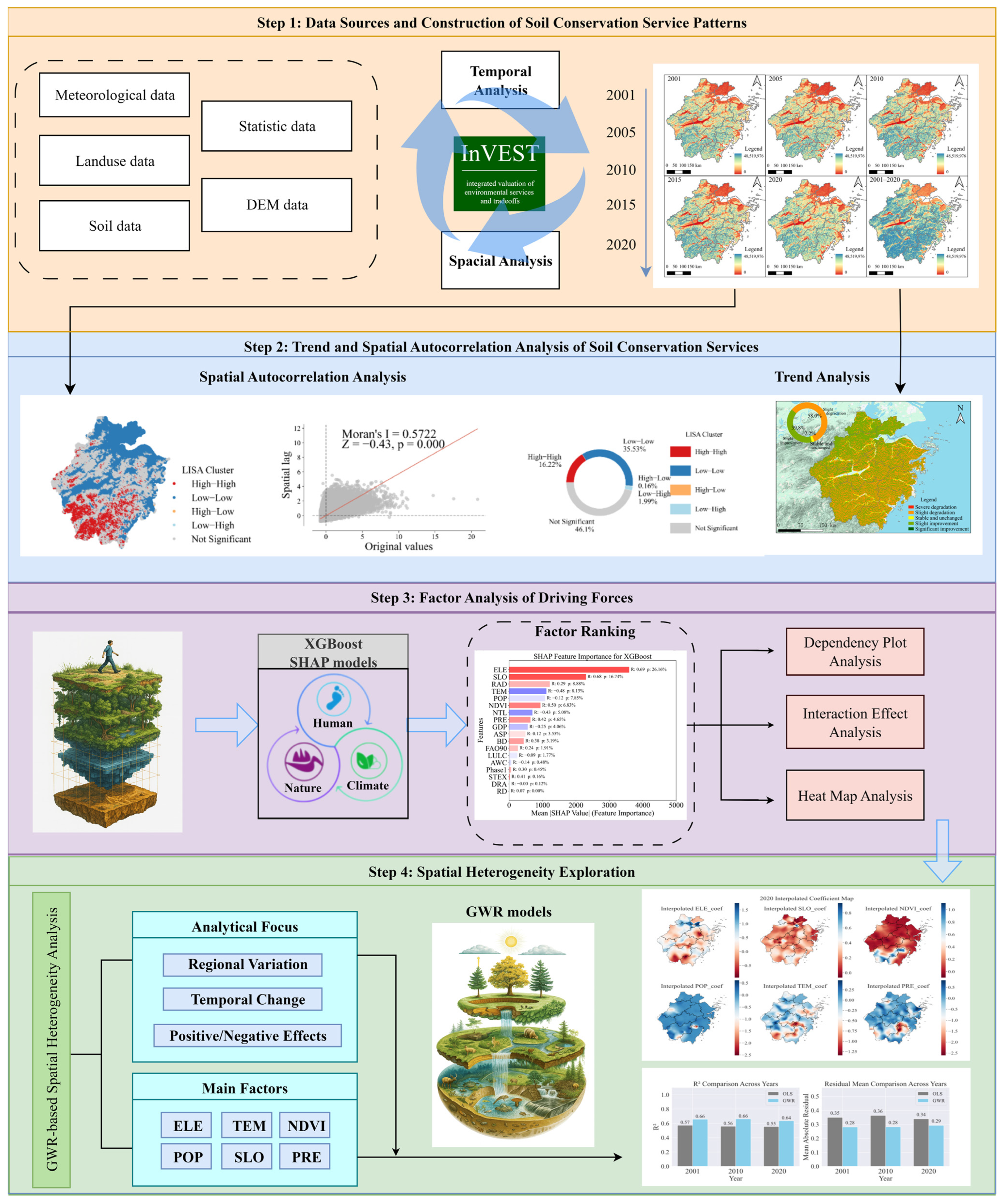
This study focuses on Zhejiang Province, a typical coastal region characterized by high human activity intensity and strong sensitivity of ecosystem services. This study aims to systematically explore the spatiotemporal evolution, spatial correlation, and driving mechanisms of SCS, as outlined in the research framework (Figure 2). First, multiple sources of data, including LULC, SLP, PRE, POP, and GDP, were collected and integrated. Second, the InVEST model was used to quantify SCS, and its spatiotemporal dynamics were examined through Sen’s trend analysis and spatial autocorrelation methods. Third, the XGBoost machine learning model was constructed to interpret the contribution of various natural and anthropogenic factors. Finally, the GWR model was applied to further reveal the spatial heterogeneity of the underlying driving mechanisms.

3.2. Methods

3.2.1. Soil Retention Capacity Calculation

In this study, the Sediment Delivery Ratio (SDR) module of the InVEST model was used to calculate soil retention at the pixel level by incorporating the Universal Soil Loss Equation (USLE) [26]. This soil retention value represents the soil conservation service (SCS), defined as the reduction in potential soil loss under natural conditions due to current land cover and management. This approach allows for the evaluation of regional soil retention capacity. The SCS can be expressed as A E X i , as detailed in the following calculation process [27].
Soil retention ( A E X i ) is defined as the difference between the potential soil erosion under natural conditions ( R K L S i ) and the actual soil erosion under current land use ( U L S E i ). The expression is as follows:
A E X i = R K L S i U S L E i
R K L S i = R i K i L S i
U L S E i = R i · K i · L S i · C i · P i
where R i denotes the erosivity of rainfall, while K i reflects the inherent susceptibility of soil to erosion. L S i accounts for the combined effects of slope length and steepness. C i represents the influence of vegetation cover and land management practices, and P i indicates the effect of soil conservation measures.
1.
Rainfall Erosivity Factor (R)
The rainfall erosivity factor is one of the key variables in the USLE model, representing the ability of rainfall to detach and transport soil particles. In this study, a monthly empirical model was used to calculate the R factor [28], with the following formula:
R = i = 1 12   1.735 × 10 [ 1.5 × l g P i 2 P 0.8188 ]
where P i represents the precipitation in month i (mm), and P denotes the total annual precipitation (mm).
2.
Soil Erodibility Factor (K)
The K factor reflects the susceptibility of soil to erosion based on its intrinsic physical and chemical properties. It is estimated using the modified EPIC (Erosion Productivity Impact Calculator) model [29], and the calculation formula is as follows:
K = ( 0.01383 + 0.51575 K e p i c ) × 0.1317
K e p i c = 0.2 + 0.3 e x p 0.0265 S A N 1 S I L 100 × S I L C L A + S I L 0.3 × 1 0.25 C C + e x p ( 3.72 2.95 C ) × 1 0.7 S N S N + e x p ( 22.9 S N 5.51 )
where S N = 1 S A N / 100 ; S A N , S I L ,   C L A   and   C represent the contents of sand, silt, clay, and organic carbon, respectively (%).
3.
Cover and Management Factor (C)
The C factor reflects the inhibitory effect of vegetation cover on soil erosion. First, the vegetation coverage f c is calculated using NDVI as follows:
C = 1         ( f c = 0 ) 0.6508 0.3436 · lg   f c         ( 0 < f c 78.3 % ) 0         ( f c > 78.3 % )
f c = ( N D V I N D V I 0 ) / ( N D V I g N D V I 0 )
where f c represents the vegetation coverage; NDVI is the Normalized Difference Vegetation Index; N D V I 0 is the NDVI value of bare soil or areas without vegetation cover; and N D V I g is the NDVI value of pixels with full vegetation cover.
4.
Support Practice Factor (P)
The support practice factor refers to the ratio of soil loss under specific soil and water conservation measures to the soil loss without any conservation practices. In this study, the P factor was assigned based on Slope conditions for different land use types and by referencing related studies conducted in similar regions [30]. The values were set as follows: cropland = 0.3, forest = 1, shrubland = 1, grassland = 0.9, water bodies = 0, barren land = 1, and impervious surfaces = 0.

3.2.2. Spatial Correlation

To investigate the spatial distribution characteristics of SCS, this study conducted a spatial autocorrelation analysis to capture both global and local patterns of spatial dependence. Global spatial autocorrelation was assessed using Moran’s I, which measures the degree to which similar values of SCS are spatially clustered across the entire study area. A significantly positive Moran’s I indicates strong spatial clustering of similar values, while a negative value suggests dispersion. The formula for global Moran’s I is as follows:
I g = n i = 1 n   x i x ¯ j = 1 n   W i j x j x ¯ i = 1 n   x i x ¯ 2 i = 1 n   j = 1 n   W i j
where n refers to the number of spatial units, while x i and x j are the observed values at grid cells i and j, respectively. The symbol x ¯ represents the overall mean of all grid values. W i j denotes the spatial weight assigned to the relationship between cells i and j. For the construction of the weight matrix, we adopted the queen contiguity criterion, which considers neighbors sharing both edges and corners.
To complement the global analysis, local spatial autocorrelation was evaluated using Local Indicators of Spatial Association (LISA). This method enables the identification of spatial clusters and outliers at a finer scale by comparing each unit with its neighboring units. The LISA results reveal specific areas exhibiting High–High or Low–Low clusters, as well as High–Low and Low–High outliers, providing valuable insight into the localized patterns of soil conservation and potential influencing factors. The formula for local Moran’s I is as follows:
I l = ( x i x ¯ ) i = 1 n   x i x ¯ 2 / ( n 1 ) j = 1 n   W i j ( x j x ¯ )
The results of the LISA analysis were classified into five spatial clustering types: High–High (hot spots), where areas with high values are surrounded by neighbors with similarly high values; Low–Low (cold spots), representing clusters of low values; High–Low and Low–High, which indicate spatial outliers with contrasting values compared to their neighbors; and Not Significant, denoting areas without statistically meaningful spatial association.

3.2.3. Trend Analysis

1.
Sen’s Slope Estimation
To quantify the long-term directional changes in the Soil Conservation Service (SCS) across Zhejiang Province from 2001 to 2020, we applied the Sen’s slope estimator. This non-parametric method is widely used in environmental studies due to its robustness against outliers and its suitability for data that may not follow a normal distribution [31,32].
S l o p e = M e d i a n [ ( ( S C S _ j S C S _ i ) ) / ( j i ) ] , 1 i j t
where S C S _ i and S C S _ j represent the observed values of the variable at time steps i and j, respectively, while t denotes the total number of temporal observations. The computed slope reflects the overall direction and magnitude of the temporal trend.
2.
Mann-Kendall Test
To assess the statistical significance of temporal trends in SCS over the period 2001–2020, we employed the M–K test, a widely adopted non-parametric method for detecting monotonic trends in environmental time series data. This test is particularly suitable for analyzing remote sensing-derived indicators due to its resilience to missing values and non-normal distributions [19]. The formula for the M–K test is provided in Supplementary Material S1.

3.2.4. Geographically Weighted Regression Model

The GWR model is a spatial analysis technique based on the Ordinary Least Squares (OLS) model, used to estimate parameters and visually represent how the influence of explanatory variables varies across different regions [33]. When there is significant spatial autocorrelation among variables, the OLS model may not meet the requirements of this study. Therefore, the GWR model is introduced, which performs local linear regressions while fully accounting for spatial non-stationarity, replacing global parameter estimates with locally estimated parameters. The performance of the GWR model is highly dependent on the choice of kernel function and optimal bandwidth. After comparative analysis, a fixed Gaussian kernel was selected, and the corrected Akaike Information Criterion (AICC), which adjusts for small-sample bias, was used to determine the optimal bandwidth in this study. The equation for the GWR fitted model is as follows:
y i = β 0 ( u i , ν i ) + k   β k ( u i , ν i ) x k , i + ε i
where y i is the observed value of sample i, and ( u i , ν i ) are the coordinates of sample i. β 0 ( u i , ν i ) is the intercept term that varies spatially with location ( u i , ν i ) . β k ( u i , ν i ) x k , i is the k-th regression coefficient at the location of sample i, and x k , i , i is the k-th independent variable for sample i; ε i is the random error term.

3.2.5. XGBoost–SHAP Algorithm and Variable Selection

To further identify the dominant factors influencing changes in SCS in Zhejiang Province and to explore their nonlinear response mechanisms, this study developed an interpretable machine learning framework that integrates XGBoost with SHAP, based on the quantitative results from the InVEST model [34]. This method not only offers high predictive accuracy but also reveals complex nonlinear relationships and interaction effects among multiple variables. It has been widely applied in fields such as ecosystem services, land use, and soil carbon storage [35,36].
XGBoost is a gradient boosting decision tree (GBDT) algorithm that constructs weak learners iteratively and minimizes residual squared error, while incorporating L1 and L2 regularization to enhance model robustness [37]. It is well-suited for modeling high-dimensional nonlinear data. In this study, the soil retention service (t·hm−2·a−1) calculated from the InVEST model for the period 2001–2020 was used as the response variable. The explanatory variables included natural and climatic factors (e.g., precipitation, temperature, solar radiation), topographic features (e.g., slope, aspect, terrain relief, elevation), and human activity indicators (e.g., land use intensity, nighttime light index, population density, and GDP) [38]. The key hyperparameters of the XGBoost model were set as follows: learning rate = 0.1, max depth = 6, number of trees = 500, subsample = 0.8, and colsample_bytree = 0.8. L1 and L2 regularization terms were applied to reduce overfitting. An early stopping strategy was used to terminate training if no improvement was observed on the validation set after 50 rounds. A 70/30 train-test split was adopted to evaluate model performance. Pearson correlation analysis was used to assess multicollinearity, and no strong correlations were found.
In order to improve the interpretability of the model, this study employed SHAP to evaluate how each input feature affects the predicted outcome [39], thereby quantifying both global importance and the direction (positive or negative) of influence. SHAP relies on Shapley value theory, which originates from cooperative game theory, to break down the model output into feature-level contributions. The core computational principle is expressed by the following formula:
φ i ( v ) = S N \ { i }   | S | ! ( | N | | S | 1 ) ! | N | ! ( v ( S { i } ) v ( S ) )
where N denotes the set of all input features, and S represents a subset of features that does not include feature i , and v ( S ) refers to the predicted value based on subset S .
Through dependence plots and interaction plots, it is possible to further reveal nonlinear turning points and critical thresholds in variable responses—for example, a significant increase in service supply when slope exceeds 15°, or a saturation of SCS when NDVI is in the 0.6–0.8 range [21]. This mechanism facilitates a transition from interpreting model outputs to understanding ecological processes [40]
The application of the XGBoost-SHAP combined method in this study not only enabled the “identification–ranking–response curve construction” of driving factors for SCS but also provided a scientific basis for soil erosion control and zonal management policy development in the mountainous and hilly areas of Zhejiang Province [41].

4. Results

4.1. Spatiotemporal Patterns of Soil Conservation Services

Figure 3 illustrates the spatial distribution characteristics of SCS in Zhejiang Province from 2001 to 2020. The results indicate that SCS exhibited marked spatiotemporal heterogeneity across the province over the study period. During the period 2001–2020, areas with high soil retention capacity were mainly concentrated in the mountainous regions of the west and south, such as southwestern and western Zhejiang. These areas largely overlapped with forest land and demonstrated strong soil conservation capacity. In contrast, the plains and urbanized regions (e.g., around Hangzhou and Ningbo) generally showed lower levels of SCS. This was especially evident in coastal zones and urban expansion areas, where SCS were relatively weak. From a temporal dimension, soil retention capacity declined in some areas between 2001 and 2015, but showed signs of recovery in certain regions by 2020. Overall, the spatial pattern of SCS in Zhejiang Province from 2001 to 2020 can be described as stable in mountainous areas, declining in plains, and partially recovering in transitional zones. These spatial dynamics reflect the impact of land-use changes and anthropogenic disturbances on ecosystem functions related to SCS.
Table 2 presents the total amount and percentage of SCS for each city in Zhejiang Province from 2001 to 2020. Overall, Lishui City consistently ranked first in the province in terms of SCS, with 52.04 million t/(hm2·a) in 2001, accounting for 37.17% of the provincial total, and still maintaining 47.30 million t/(hm2·a) in 2020, representing 34.04%. This highlights the significant advantage of mountainous areas. Wenzhou and Hangzhou followed closely behind. Wenzhou recorded 21.49 million t/(hm2·a) in 2001 and 17.19 million t/(hm2·a) in 2020, while Hangzhou’s SCS increased from 17.87 million t/(hm2·a) to 23.30 million t/(hm2·a), with its share rising to 16.77%, indicating an enhancement in SCS in recent years. Quzhou and Jinhua also exhibited relatively high SCS, both exceeding 10 million t/(hm2·a). In contrast, Zhoushan, Jiaxing, and Huzhou reported lower soil retention levels, with Zhoushan only reaching 0.117 million t/(hm2·a) by 2020. Overall, the spatial distribution of SCS across the cities is closely related to their topography. Cities located in mountainous regions exhibit significantly stronger SCS than those in plains and coastal areas.
Figure 4 illustrates the influence of topographic factors on SCS in Zhejiang Province. Figure 4a presents a radar chart of S SCS variability (SCS_mean) under different aspect categories. The results indicate significant spatial heterogeneity of SCS across different slope aspects, with higher SCS_mean values observed in the northeast- and northwest-facing slopes. This suggests that the aspect can modulate SCS by influencing microclimatic conditions such as solar radiation and moisture availability. Figure 4b shows the relationship between slope and SCS variability. As the slope increases, SCS_mean exhibits a clear upward trend, peaking in the steepest slope category. This indicates that areas with steeper slopes tend to have stronger spatial variability in SCS, likely due to higher soil erosion risk and more complex hydrological processes. Additionally, areas with low slopes account for the largest proportion of pixels, indicating that the study region is predominantly characterized by gentle terrain. Figure 4c analyzes SCS variability across different elevation intervals. The results show that SCS_mean gradually increases with elevation, reaching its highest value in high-altitude areas. This trend suggests that mountainous regions exhibit greater spatial heterogeneity in SCS, potentially influenced by complex terrain, vegetation types, and climatic gradients. However, the majority of pixels are distributed in low-elevation zones, indicating that low-altitude areas are more widespread across the region.
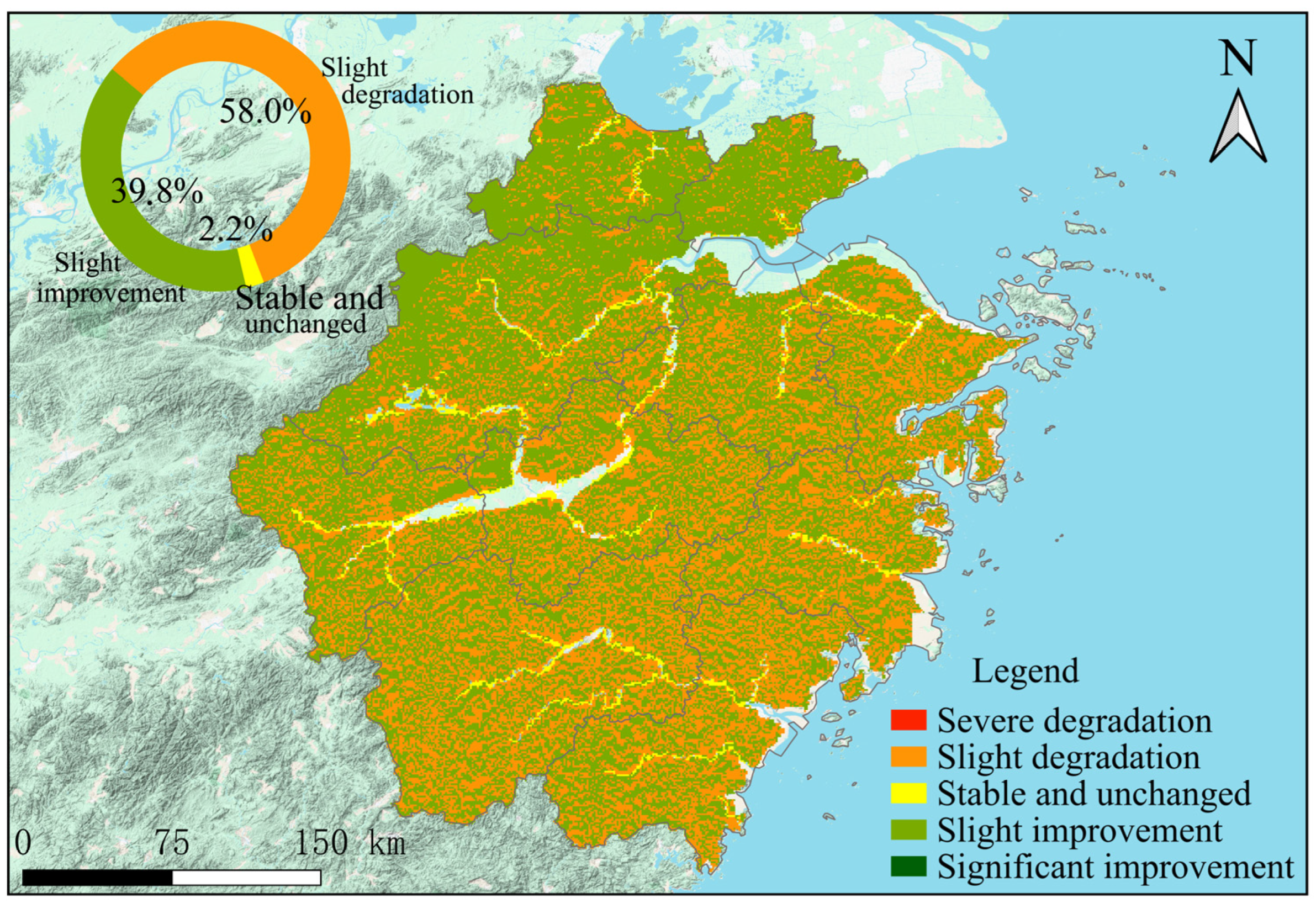
Figure 5 shows the spatial distribution of soil retention trends in Zhejiang Province from 2001 to 2020, based on Sen’s slope trend analysis and M–K test significance testing. In terms of area proportion, stable areas dominate, accounting for approximately 58.05%, mainly located in the western and southern mountainous regions of Zhejiang. These areas exhibit strong ecological stability due to favorable natural conditions and high vegetation coverage. Slightly degraded areas make up 39.78%, primarily concentrated in the northern and coastal plain areas of Zhejiang, which are closely associated with intensive human activities and urban expansion. Severely degraded areas are limited in extent, comprising only 2.18% of the total area, but they pose a high ecological risk. These areas are mainly distributed around urban fringes and transportation corridors, and they represent priority zones for future ecological restoration efforts. The overall average Sen’s Slope value is −1203.17, indicating a slight declining trend in soil retention across the province. At the subregional level, severely degraded areas exhibit a strong negative trend, with an average slope of −165,186.8. In contrast, stable areas have an average rate of change close to zero. Improved areas show a clear increasing trend, with an average slope of 111,087.9, suggesting that soil retention functions in mountainous and ecologically restored areas have improved to some extent. The spatial trend of SCS in Zhejiang Province can be summarized as improvement in mountainous regions, degradation in plains, and overall stability at the provincial scale. This pattern highlights the significant influence of land use change and human activity intensity on regional ecosystem services. The results provide a scientific basis for targeted ecological protection, degradation management, and restoration of key areas.

4.2. Spatial Autocorrelation Analysis

Figure 6 presents the results of spatial autocorrelation analysis of SCS in Zhejiang Province for the years 2001, 2005, 2010, 2015, and 2020, including LISA cluster maps, Moran scatter plots, and LISA cluster proportion pie charts. Overall, SCS in Zhejiang Province exhibited significant positive spatial autocorrelation in all years, with Global Moran’s I values remaining stable at approximately 0.57 (e.g., 0.5696 in 2020), and significance tests passed in all cases (p = 0.000). This indicates a strong spatial clustering pattern of SCS. The LISA cluster maps further reveal the spatial distribution of clustering types. High–High clusters are mainly concentrated in the mountainous areas of southwestern Zhejiang, such as Lishui and Quzhou, reflecting the strong soil retention capacity and high ecosystem stability of these regions. In contrast, Low–Low clusters are primarily distributed around urban expansion zones and coastal plains in cities like Hangzhou and Ningbo, indicating areas with intense land development and weaker ecological function. The spatial heterogeneity represented by High–Low and Low–High clusters is relatively limited, accounting for less than 2% in all years, suggesting that extreme heterogeneity in soil retention values is minimal and that the regional structure remains relatively stable. According to the pie charts, the proportion of High–High clusters remained essentially stable from 2001 to 2020 (around 16.22%), while the proportion of Low–Low clusters slightly increased (from 33.95% to 34.45%). Meanwhile, the proportion of non-significant areas slightly decreased (from 46.1% to 47.13%), indicating a slight enhancement in spatial clustering in some areas. In summary, SCS in Zhejiang Province has consistently maintained a clear spatial clustering pattern over the past two decades. The mountainous regions in the southwest are key providers of ecosystem services and should continue to be protected. In contrast, coastal and plain areas require strengthened soil and water conservation measures to improve overall ecosystem function and resilience.

4.3. Driving Force Analysis of Soil Retention

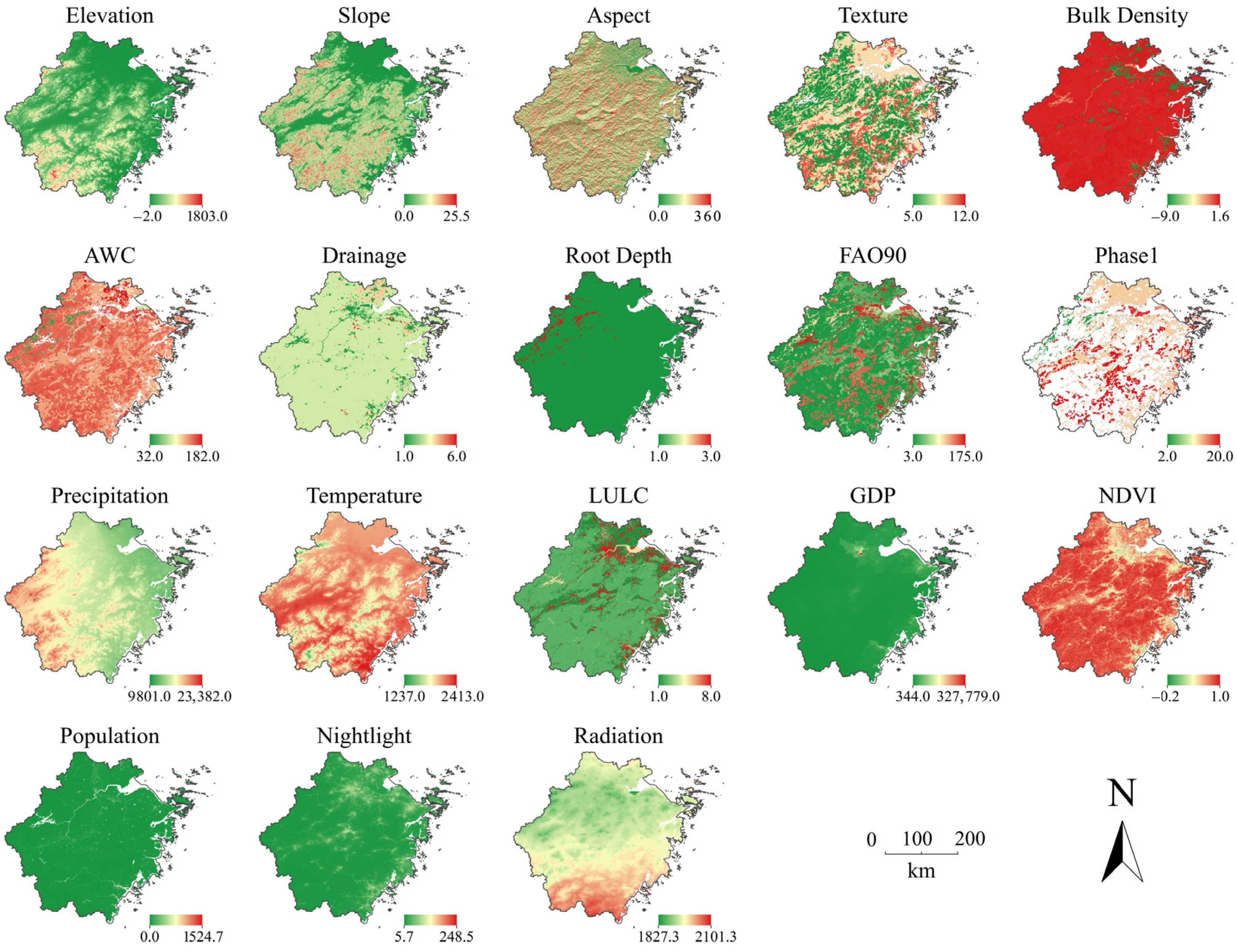
Figure 7 illustrates the spatial distribution patterns of the major natural and socio-economic factors involved in the driving force analysis of soil retention in Zhejiang Province. These factors fall into five categories—topography, soil, climate, land use, and human activities—and include a total of 17 specific indicators. Among the topographic factors, elevation, slope, and aspect show distinct east–west differences, with higher elevations and steeper slopes concentrated in the western mountainous regions, providing favorable natural conditions for soil retention. For soil-related factors, texture, bulk density, available water capacity (AWC), drainage, root depth, FAO90 soil classification, and soil phase (Phase1) exhibit complex and diverse spatial variation, playing key physical and chemical regulatory roles in the soil retention process. In terms of climate factors, precipitation and temperature display clear latitudinal gradients—higher in the southwest and lower in the northeast—affecting both soil erosion and vegetation growth dynamics. The spatial patterns of LULC and NDVI reflect the impact of land management practices and vegetation cover conditions on soil retention. Socio-economic factors include GDP, population density, nighttime light, and radiation. These indicators reveal the spatial intensity of human activities, with GDP and nighttime light data showing particularly high values in coastal areas and urban agglomerations, indicating strong anthropogenic disturbances and potential ecological threats. Overall, the combined influence of these factors shapes the spatial patterns and dynamics of SCS in Zhejiang Province. In the subsequent analysis, the contributions of these variables will be quantified using machine learning models such as XGBoost and SHAP analysis. This approach will help identify the dominant drivers and key impact areas, thereby providing scientific support for formulating targeted ecological conservation strategies and land-use policies.

4.3.1. Overall Analysis

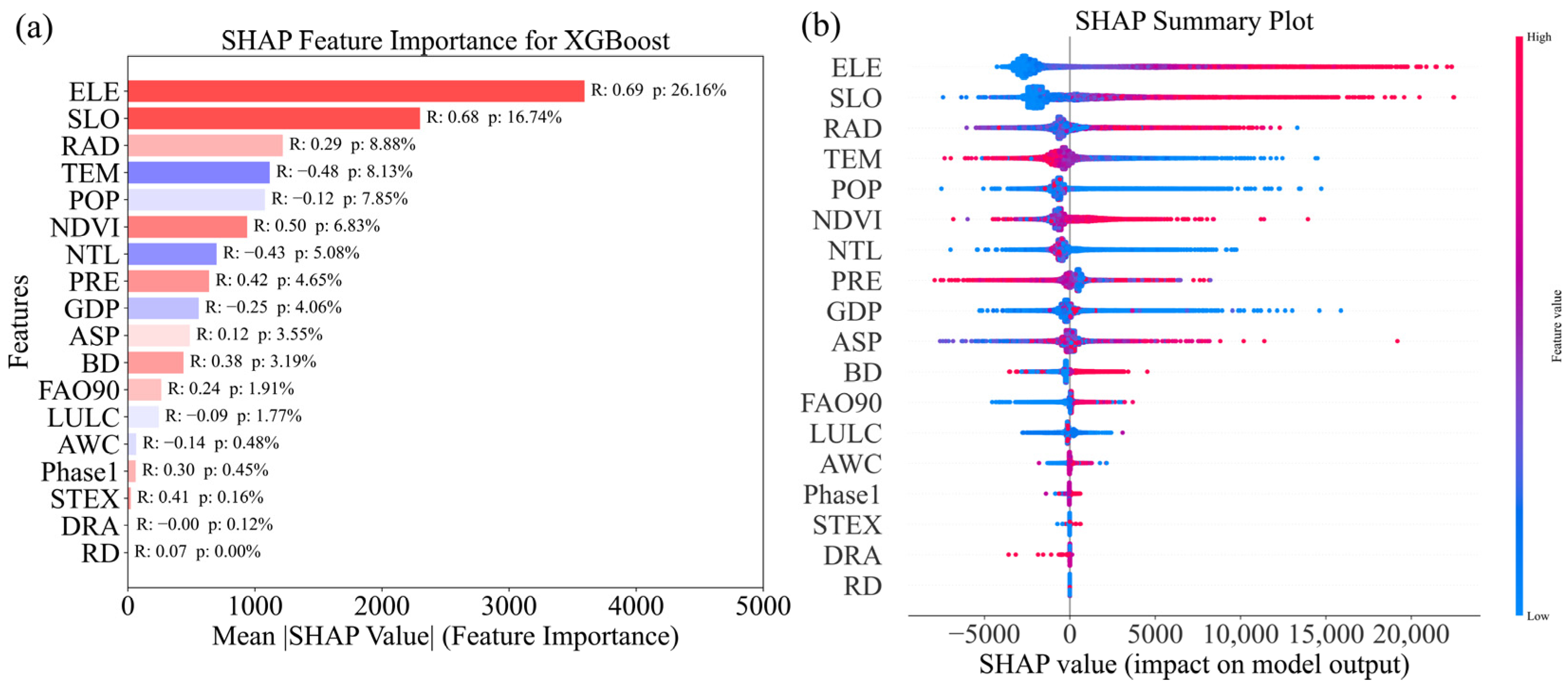
Based on the training results of the XGBoost model, this study employed the SHAP method to calculate the SHAP values of each driving factor, thereby quantitatively evaluating the marginal contribution of each variable to the spatial distribution of SCS. Before conducting SHAP-based interpretation, the predictive performance of the XGBoost model was evaluated to ensure reliability. A 70/30 train-test split was adopted. The model achieved an R2 of 0.6915 on the training set and 0.6151 on the test set. The small gap in R2 (0.0764) indicates no severe overfitting and demonstrates good generalization performance. Subsequently, the relative contribution of each factor was computed as a percentage of the total SHAP values (Figure 8a), enabling an objective ranking of factor importance and revealing the driving mechanisms of SCS in Zhejiang Province. As shown in Figure 8a, the top five most important factors are elevation (26.16%), slope (16.74%), solar radiation (8.88%), temperature (8.13%), and population density (7.85%). Among them, elevation had the highest influence weight, with a Pearson correlation coefficient of R = 0.69 (p < 0.001), indicating that higher elevation significantly enhances soil retention capacity. The western mountainous regions, characterized by rugged terrain and high vegetation coverage, exhibit stronger ecological stability. Slope ranked second, with its high SHAP value highlighting its crucial role in increasing surface roughness and reducing runoff velocity on sloped terrains. Among climatic factors, both RAD and TEM were identified as major drivers, showing varying ecological responses. Solar radiation affects SCS primarily by regulating vegetation growth, which alters NDVI values and, in turn, the C factor in the USLE model. Higher radiation typically promotes canopy development, enhancing soil retention capacity through improved vegetation cover. Temperature had an overall negative effect on soil retention (R = −0.48), which may be attributed to intensified heat stress and vegetation degradation in low-altitude urbanized areas. POP and nighttime light index, both indicators of human activity intensity, showed negative contributions, with correlation coefficients of R = −0.50 and R = −0.43, respectively. This suggests that urban expansion and land development are major external pressures contributing to the degradation of SCS in Zhejiang.
The SHAP summary plot shown in Figure 8b visually displays the direction and magnitude of each variable’s contribution across its value range. The results show that high values of elevation, slope, and NDVI are associated with positive SHAP values, indicating that increases in these natural factors can effectively enhance SCS. In contrast, high values of GDP, nightlight, and temperature tend to correspond to negative SHAP values, highlighting their strong association with service degradation. Additionally, variables such as bulk density, aspect, and FAO90 exhibit relatively narrow SHAP value distributions, suggesting that their influence is weaker and spatial heterogeneity is less pronounced at the provincial scale. In summary, the SHAP method enables transparent interpretation and scientific ranking of driving factors. The findings confirm the dominant role of natural topographic factors in shaping the spatial pattern of SCS, while also emphasizing the disruptive effects of human activities on ecosystem services. These results provide a basis for developing differentiated conservation policies in ecologically sensitive areas and offer theoretical support for regionalized governance and soil retention strategies in both mountainous and coastal zones.

4.3.2. Analysis of Key Factor Response Mechanisms Based on SHAP Dependence Plots

Building on the key factors identified in the previous section, this study further generated SHAP interaction plots for the top seven ranked variables (Figure 9) to reveal the nonlinear effects and interactions among variables, thereby providing a more comprehensive understanding of the driving mechanisms behind SCS.
As shown in Figure 9, elevation, slope, and RAD are the three most influential natural factors, each exhibiting significant interactive contributions. The interaction between elevation and slope is particularly notable. In areas with both high elevation and steep slopes, SHAP interaction values are generally positive, indicating that the synergistic effect of these two variables greatly enhances SCS. This underscores the role of complex terrain and rich vegetation in mountainous areas in reinforcing soil conservation. Conversely, in low-slope or low-elevation regions, this synergy tends to be negative, suggesting limited soil retention capacity in plains and the need for enhanced ecological restoration and management efforts. In the interaction plot between RAD and NDVI, NDVI’s contribution to soil retention increases significantly under moderate solar radiation (~15,000 MJ·m−2), while the effect stabilizes in areas with low or extremely high radiation levels. This indicates that optimal solar conditions promote vegetation growth, which in turn enhances soil retention capacity. Among human activity factors, the interaction between population density and nighttime light reveals a strong negative effect. In areas with both high population density and intense nighttime lighting, SHAP values are predominantly negative, reflecting the combined negative impacts of urban expansion, land surface sealing, and ecosystem fragmentation on SCS. This finding is consistent with previous conclusions and suggests that urban areas should prioritize the development of ecological buffer zones and green infrastructure. Additionally, temperature shows complex nonlinear interactions with natural factors such as elevation and slope. In moderate to low-temperature regions (<18 °C), temperature increases are positively associated with the SHAP values of these natural factors, thereby promoting SCS. However, in high-temperature regions, this relationship tends to level off or even become negative, indicating that heat stress under climate change may suppress ecosystem functionality. In summary, the SHAP interaction analysis reveals the nonlinear responses and spatial coupling mechanisms among key driving factors, particularly in mountainous areas and urban fringes. The combined effects of topography, climate, and human activity shape the spatiotemporal differentiation of SCS and provide theoretical support for targeted policy-making and ecological zoning strategies.

4.3.3. Analysis of Interaction Mechanisms Among Driving Factors

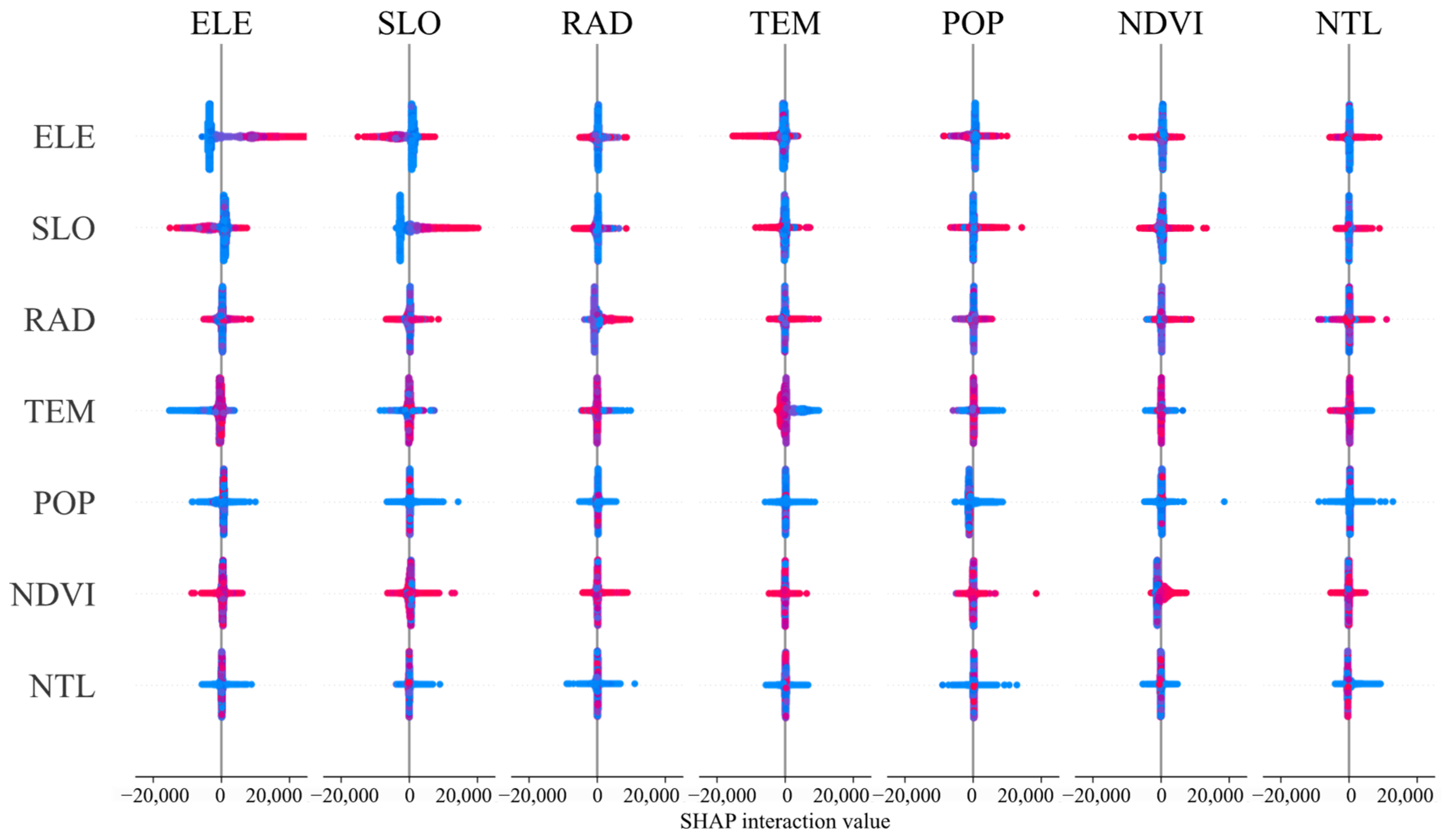
Analyzing the effect of individual variables alone often fails to fully capture the nonlinear nature and interaction characteristics of the system. Therefore, this study further generated SHAP interaction plots between the main driving factors (Figure 10) to visualize how variable interactions influence SCS. In Figure 10, the horizontal axis represents the SHAP interaction values, indicating the strength and direction of interactions between variables—the farther from the centerline, the more significant the interaction effect. The vertical axis lists the variable names involved in each interaction, and the density of the plotted points reflects the consistency of the model’s predictions for that interaction. A denser distribution implies a more stable prediction between the interacting variables, whereas a more scattered distribution suggests higher uncertainty. The interaction plot reveals that the most significant interactions occur between elevation ∩ slope, population density ∩ elevation, and slope ∩ NDVI. The interaction between elevation and slope is concentrated in the positive region, indicating that these two variables synergistically enhance soil retention capacity under mid- to high-mountain conditions. This aligns with the characteristics of the hilly and mountainous regions in western Zhejiang, where rich vegetation, rugged terrain, and effective erosion control contribute to strong soil retention performance. In the interactions between human activity and natural factors, the population density ∩ elevation combination exhibits a complex response. In mid- to high-elevation areas with low population density, the interaction is mostly positive, indicating that ecosystems maintain good soil retention capacity under limited human disturbance in mountainous regions. In contrast, in low-elevation areas with high population density, the interaction tends to be negative, suggesting that urbanization intensifies the degradation of SCS—especially in the coastal zones of the Yangtze River Delta. Moreover, the interaction between slope and NDVI also displays a notable nonlinear structure. In areas with slopes greater than 15° and high NDVI values (>0.6), the SHAP interaction values are generally positive, indicating stronger soil retention capacity in regions with good vegetation cover and complex terrain. Conversely, in areas with low slope and low NDVI, the interaction turns negative, reflecting the adverse impact of lowlands, bare land, or impervious urban surfaces on SCS. Overall, the SHAP interaction plots reveal positive coupling mechanisms among natural factors—for example, combinations such as “high slope + high NDVI” or “high elevation + low nighttime light” significantly enhance SCS. In contrast, combinations such as “high population density + high nighttime light” or “low slope + low NDVI,” which represent areas with intense human disturbance, exhibit negative synergistic effects. These findings have important policy implications. For example, in areas with high elevation and low nightlight values, where human disturbance is minimal, the priority should be to maintain existing vegetation and prevent new development. These regions provide strong soil conservation services and play an ecological buffering role. In contrast, low-elevation areas with high population density, often located in urban and coastal zones, require measures such as green infrastructure, slope protection, and stricter land-use control to mitigate degradation. In agricultural regions with moderate slope and vegetation, promoting eco-friendly farming and vegetation buffer zones can further enhance soil retention. These interaction patterns provide new insights into the mechanisms through which multiple factors influence ecosystem services and offer scientific references for implementing differentiated ecological management and land-use planning in the future.

4.3.4. Heat Map Analysis of SHAP Values

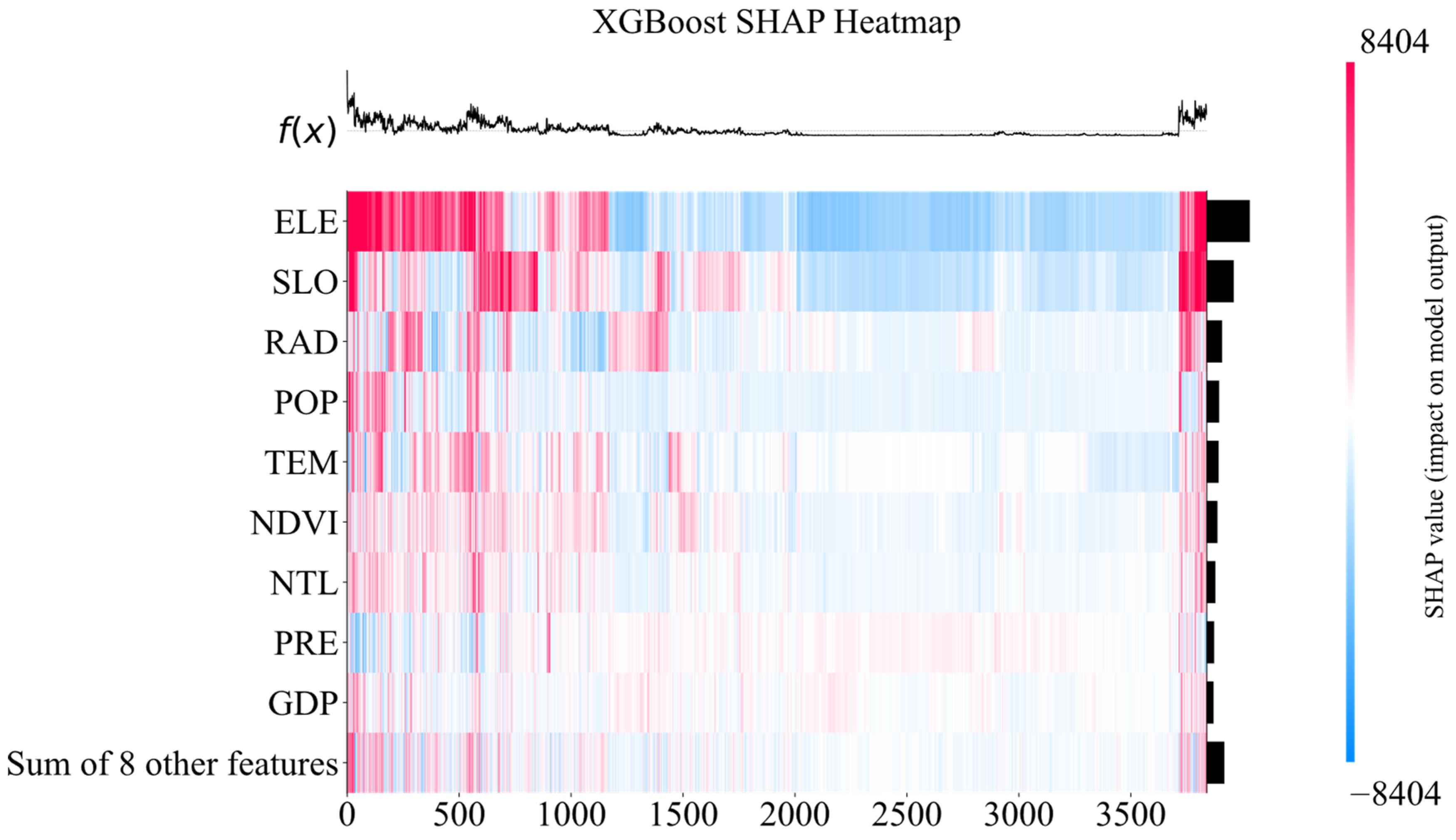
To further identify the overall influence patterns of driving factors on SCS, this study generated a SHAP value heat map (Figure 11), which intuitively illustrates the contribution direction and magnitude of each variable at the sample level. The color scale ranges from blue (negative impact) to red (positive impact), revealing the heterogeneous contributions of different factors across spatial units. From the overall distribution, socio-economic factors such as population density (Population), GDP, and nighttime light exhibit relatively high SHAP values in most samples, indicating a stronger driving effect on SCS. Their contributions are predominantly negative, emphasizing the significant suppressive impact of urbanization on ecosystem service functions. This trend is particularly evident in the upper part of the heat map, reflecting that areas with intense human activity tend to have weaker soil retention service capacity. However, the heat map also shows that natural factors such as elevation, slope, and NDVI generally exhibit lower SHAP values but contribute significantly and positively in certain samples. This indicates that natural geographical conditions still play a critical supporting role in specific regions. In mountainous areas with pronounced terrain variation, the composite landforms formed by these factors enhance surface stability and soil and water conservation capacity. Notably, some variables show clear bidirectional effects. For instance, population density (pop) and TEM display both positive and negative SHAP values across different samples, reflecting that their impacts are not fixed but dynamically adjust depending on the regional context. For example, in some peripheral mountainous regions, moderate population density may be associated with ecological restoration or agricultural management investments, thereby positively influencing soil retention capacity. In contrast, in urban expansion areas, these variables typically show negative effects. In summary, the SHAP heat map analysis indicates that the driving mechanisms of ecosystem services exhibit significant spatial heterogeneity and nonlinear response characteristics. Therefore, it is not appropriate to generalize the ecological effects of variables based solely on overall trends; rather, their impacts should be interpreted in conjunction with regional features and geographical context to capture their variability and complexity. This analysis provides valuable data support and decision-making references for achieving a balance between ecological conservation and urban development.

4.4. Spatial Heterogeneity Analysis of Key Influencing Factors

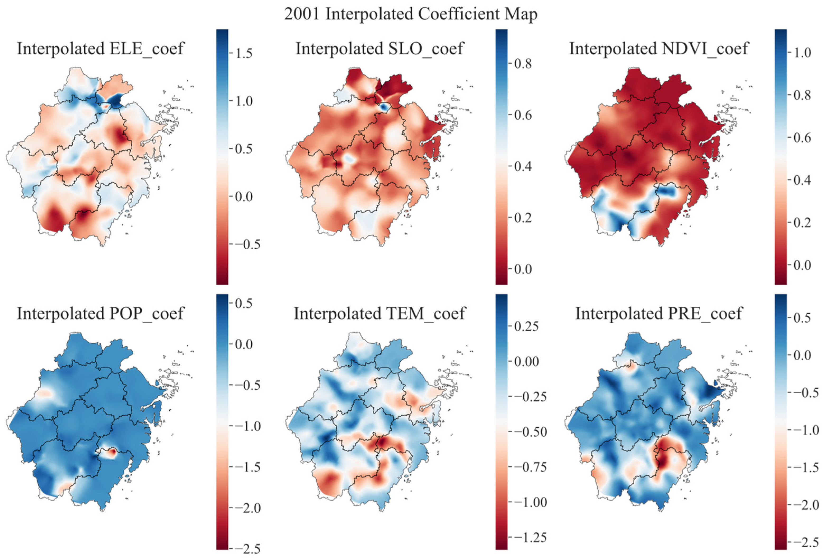
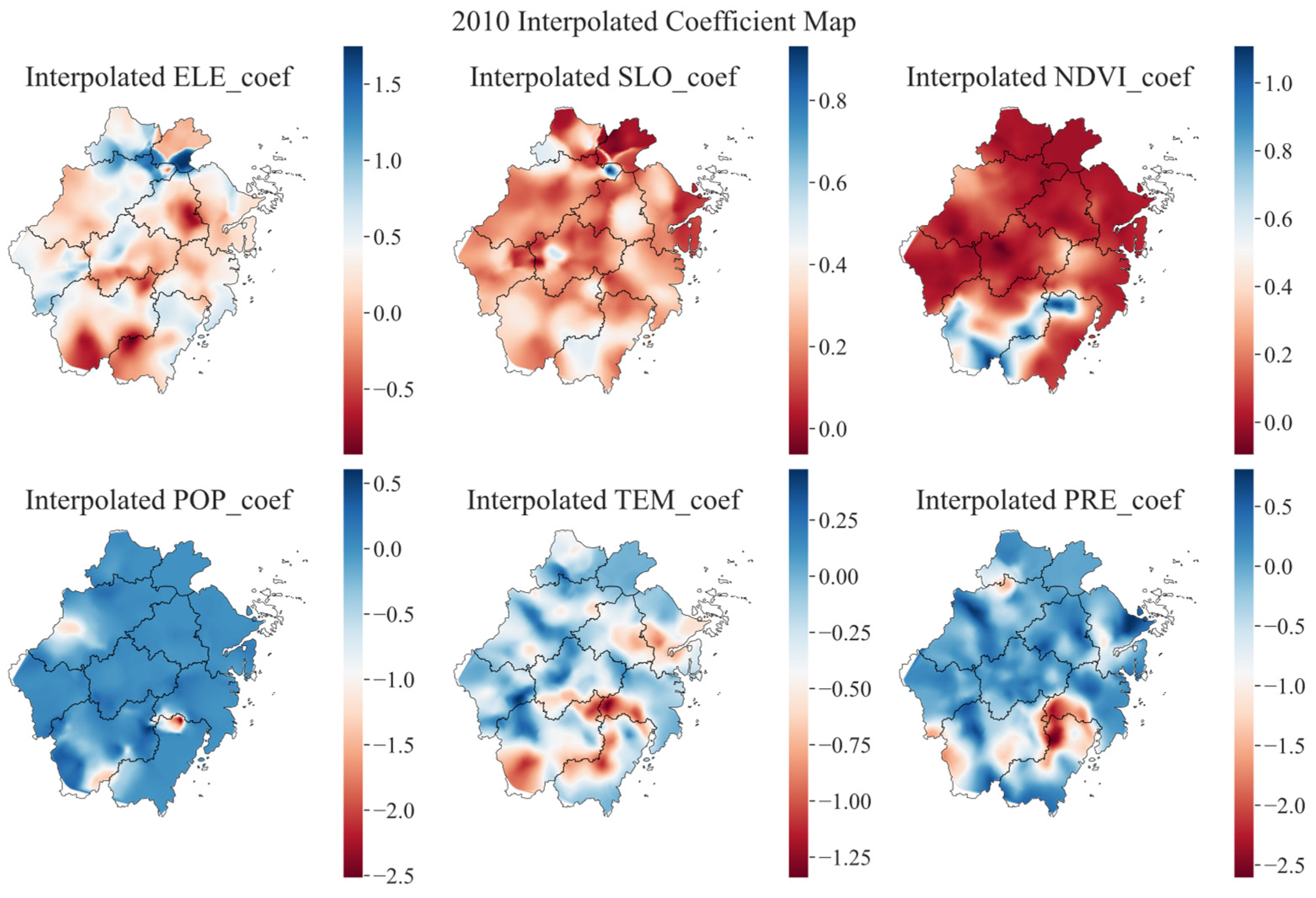
Figure 12, Figure 13 and Figure 14 display the spatial interpolation of coefficients for the main driving factors—elevation, slope, NDVI, population density (pop), TEM, and precipitation (pre)—based on GWR models for the years 2001, 2010, and 2020. These coefficients represent the local direction and strength of each factor’s influence on SCS. Across all three years, the coefficient of elevation is generally positive in the mountainous areas of western Zhejiang (e.g., Lishui, Quzhou, western Jinhua), indicating that high-elevation areas benefit significantly from improved SCS. In contrast, coefficients in the coastal plain regions are close to zero or even negative, suggesting that flatter areas contribute less to soil retention and may even be adversely affected by development pressures. Slope shows a consistently positive effect throughout the study period, particularly in the western mountainous regions. Compared to 2001, the positive influence of Slope expands toward central Zhejiang in 2010 and 2020, indicating an increasing spatial extent of Slope’s contribution to SCS over time. NDVI demonstrates a significant positive effect province-wide, with the strongest influence observed in the central and western mountainous areas. In contrast, coefficients are lower or even slightly negative in coastal and urban areas, highlighting vegetation cover as a core driver of enhanced soil retention capacity.
The coefficient for population density is overall negative, especially in urban agglomerations such as Hangzhou, Ningbo, and Wenzhou. This reflects the suppressive effect of intense human activities on SCS. While the negative influence of population was relatively limited in 2001, it gradually expanded by 2010 and 2020, underscoring the increasing ecological pressure from urbanization. Temperature shows considerable spatial variability across different years. In 2001, the coefficients were negative in northern and coastal Zhejiang but positive in the southern mountainous areas. By 2010 and 2020, the zones of negative influence expanded into parts of central Zhejiang, suggesting that rising temperatures may be exacerbating ecological vulnerability in low-elevation regions. Precipitation coefficients are generally positive, concentrated in southern and western Zhejiang, where abundant rainfall supports vegetation growth and enhances soil retention through positive feedback mechanisms. Compared with 2001, the positive influence of precipitation expanded in 2010 and 2020, indicating an increasing role of climatic factors in SCS. Overall, natural terrain and vegetation factors (such as elevation, slope, and NDVI) have consistently dominated the spatial pattern of SCS in Zhejiang Province over time. In contrast, the influence of socio-economic and climatic variables such as population and temperature has shown notable temporal dynamics and regional variation. These findings provide important insights for implementing region-specific management strategies, optimizing human–environment relationships, and formulating differentiated ecological protection policies in Zhejiang Province.

5. Discussion

5.1. Correlation Between Soil Retention and Driving Factors

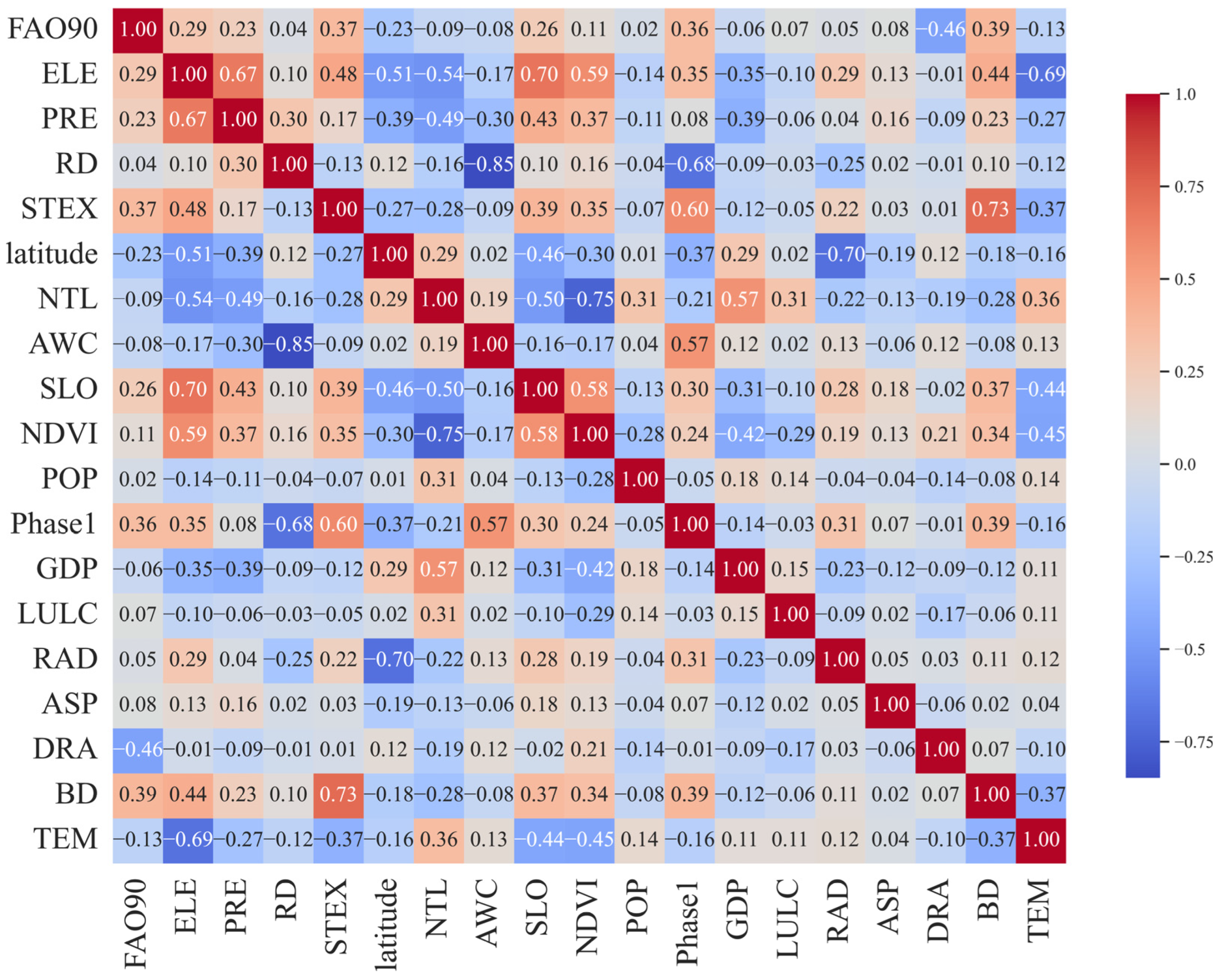
The correlation analysis in this study revealed significant relationships between soil retention and various natural, climatic, and anthropogenic factors (Figure 15). Overall, elevation, slope, and NDVI showed strong positive correlations with soil retention, indicating that terrain variability and vegetation cover are core natural drivers for maintaining and enhancing SCS [42]. In contrast, human activity intensity indicators such as population density, GDP, and nighttime light showed weak correlations with these natural factors, highlighting the independent influence and potential threat posed by anthropogenic disturbances on ecosystem services [43]. Additionally, precipitation was positively correlated with elevation and negatively correlated with temperature, reflecting the distinct north–south climatic gradient of Zhejiang Province. These key findings provide a theoretical foundation for subsequent driver analysis and spatial modeling. The mechanisms underlying these correlations suggest that topographic conditions and vegetation cover jointly determine the susceptibility to soil erosion and the capacity for soil retention [42]. Areas with high elevation, steep slopes, and high NDVI—mostly located in the central and western mountainous regions—benefit from favorable natural conditions and limited human disturbance, thus exhibiting stronger soil retention capacity. In contrast, coastal and urban areas characterized by high population density and economic development experience significant surface disturbance from activities such as urban expansion and agricultural development, which in turn reduce SCS [44]. This pattern is validated by the correlation heatmap, where, for example, the relatively high correlation between GDP and nighttime light (r = 0.57) reflects the pressure exerted by socio-economic development on ecosystem functions [45]. Compared with previous studies, the findings of this research are consistent with most conclusions related to ecosystem services. For instance, Luo et al. [46] demonstrated that mountainous areas possess higher soil and water conservation capacity due to complex terrain and abundant vegetation, while plains and urban areas are more ecologically vulnerable due to intense development. This study not only supports those conclusions but also further reveals the relatively independent correlation patterns between human activity factors and natural factors, emphasizing the importance of coordinated management of human–environment systems.

5.2. Geographically Weighted Regression vs. Ordinary Least Squares Regression

This study compared the performance of the GWR model and the OLS model in analyzing the driving forces of soil retention in Zhejiang Province. The results indicate that the GWR model significantly outperforms the OLS model in both model fit and residual error across all examined years. Specifically, the GWR model achieved higher R2 values (0.66 in 2001 and 2010, 0.64 in 2020) compared to the OLS model (0.57, 0.56, and 0.55, respectively). It also yielded lower mean absolute residuals (0.28, 0.28, and 0.29) than OLS (0.35, 0.36, and 0.34), demonstrating its stronger ability to capture spatial heterogeneity and improve predictive accuracy (Figure 16).
The superior performance of GWR can be attributed to its capacity to model spatially varying relationships, which the global OLS model cannot achieve [47]. For instance, GWR results revealed that slope and NDVI had strong positive effects on soil retention in mountainous regions, while population density and temperature exerted negative influences in urban areas. Moreover, the spatial distribution of GWR coefficients from 2001 to 2020 showed an expanding influence of natural factors and a gradual spread of negative anthropogenic impacts toward central Zhejiang [48]. These findings are consistent with previous research, and this study further extends their conclusions by providing a long-term comparative analysis. However, the GWR model remains computationally demanding and sensitive to parameter selection, indicating areas for future methodological improvement.

5.3. Management Recommendations

Considering the temporal changes and spatial drivers of SCS observed in Zhejiang Province from 2001 to 2020, several practical recommendations for ecological management are outlined below.
Priority should be given to the protection and management of ecological functional zones in the western mountainous areas, which serve as core regions for SCS and exhibit significant High–High clustering characteristics and strong ecological barrier functions [49]. Ecological projects such as natural forest conservation, reforestation and grassland restoration on marginal lands, and the construction of ecological public welfare forests should be continuously promoted to prevent land degradation and overexploitation, thereby enhancing soil and water conservation capacity [50].
At the same time, the eastern coastal and plain areas show relatively low levels of SCS and are significantly affected by urban expansion and infrastructure development, displaying a clear trend of degradation [51]. It is therefore urgent to strengthen land use management and ecological restoration in these regions. Measures should include optimizing the layout of construction land, strictly controlling the unreasonable occupation of forestland and arable land, enhancing the construction of urban green space systems and ecological buffer zones, and promoting rigid protection of ecological land through coordinated spatial planning (“multi-plan integration”).
Additionally, region-specific and differentiated management strategies should be implemented. The GWR analysis revealed spatial heterogeneity in the influence of driving factors [52]. Areas dominated by natural factors should prioritize ecological protection and natural regeneration, while regions significantly impacted by human activities should focus on implementing ecological compensation, controlling non-point source agricultural pollution, and developing green infrastructure. Management actions should align with spatial characteristics at the county level, promoting a “one region, one policy” approach for refined ecological governance [53].
Finally, it is recommended to introduce dynamic monitoring and intelligent decision-support systems into future ecological governance. Establishing a long-term monitoring platform based on remote sensing and model integration would enable real-time tracking of soil retention service trends [54]. Incorporating methods such as GWR and machine learning can support the identification of ecosystem service regulation pathways and provide scientific backing for precise and efficient ecological restoration and land-use decision-making.

5.4. Limitations and Future Perspectives

This study investigated the spatiotemporal dynamics and driving forces of SCS in Zhejiang Province using a comprehensive approach that integrated the InVEST model, GWR, and XGBoost. It systematically analyzed the spatial patterns of soil retention functions from natural, climatic, and human activity dimensions, and quantified the impact of key driving factors. The findings provide comprehensive scientific support for regional ecological protection and sustainable land management [55]. This research not only identified the critical factors influencing soil retention in Zhejiang but also offered valuable theoretical insights into the spatial heterogeneity of ecosystem services.
Nevertheless, several limitations remain and should be addressed in future research. First, the values for the C and P factors in the InVEST model were based on empirical values from the literature [56]. While this is a common simplification, it may not fully capture the localized soil and land management characteristics of the study area. Therefore, future studies could benefit from calibrating these parameters using field data to enhance model accuracy. In addition, the GWR results may be influenced by the choice of spatial weighting functions and the density of sampling points, which could affect the stability of local estimates. Second, due to data availability constraints, some input variables were represented by city- or province-level averages, which may obscure fine-scale spatial variations within the study area [57]. Third, this study employed a 3 km grid as the spatial resolution for input data integration and modeling. While this approach facilitates data integration and reduces computational demand, it may smooth out fine-scale heterogeneity, particularly in complex terrain or heterogeneous land cover types. Future research could consider multi-scale or hierarchical analyses to better capture spatial patterns at different resolutions.
Additionally, this study primarily focused on quantifying the relationships between natural and anthropogenic factors, while relatively limited attention was given to human governance elements such as policy interventions, ecological engineering projects, and social management [58]. Addressing these aspects in future research will contribute to a more holistic understanding of ecosystem service dynamics and support the design of more comprehensive and effective environmental policies.

6. Conclusions

Based on remote sensing interpretation data, this study systematically evaluated the spatiotemporal variations, trends, spatial correlations, and driving mechanisms of SCS in Zhejiang Province from 2001 to 2020 by integrating the InVEST model, Sen’s Slope estimator, M–K trend test, Moran’s I index, XGBoost with SHAP interpretation, and GWR. The study comprehensively revealed the evolution characteristics of SCS under the combined influence of natural and socio-economic factors. These findings not only enhance the scientific understanding of soil retention service dynamics at the regional scale but also provide important decision-making support for ecological conservation and sustainable land resource utilization. The main conclusions are as follows:
(1)
From 2001 to 2020, SCS in Zhejiang Province showed a fluctuating trend of “decline followed by increase.” The western mountainous areas exhibited significantly higher service levels than the eastern coastal and plain regions. Approximately 58% of the area remained stable, while around 40% experienced degradation, indicating an overall stable spatial pattern.
(2)
Moran’s I analysis indicated significant spatial clustering of SCS, with High–High clusters mainly distributed in the western mountainous areas and Low–Low clusters found in the eastern coastal and urban expansion zones. The XGBoost + SHAP analysis revealed that natural factors (elevation, slope, and NDVI) made the greatest contributions to SCS, followed by climatic and human activity factors.
(3)
GWR analysis revealed the spatial heterogeneity of the driving factors. The positive effects of natural factors were mainly concentrated in mountainous regions, while the negative effects of human activity factors were prominent in coastal cities and densely populated areas.
In summary, this study establishes an integrated analytical framework that offers a powerful tool for understanding the driving mechanisms, spatial patterns, and evolution of regional SCS. It also provides valuable scientific references for ecological protection, watershed management, and land-use optimization in Zhejiang Province and similar regions.

Supplementary Materials

The following supporting information can be downloaded at: https://www.mdpi.com/article/10.3390/rs17162865/s1.

Author Contributions

Conceptualization, Z.Q. and D.D.; formal analysis, Z.Q. and D.D.; software, Z.Q. and D.D.; resources, Z.Q., D.G. and M.Z.; writing—original draft preparation, Z.Q.; methodology, Z.Q. and D.D.; data curation, D.G.; visualization, D.G. and D.D.; investigation, M.Z.; project administration, D.D.; writing—review and editing, D.D. All authors have read and agreed to the published version of the manuscript.

Funding

This research was funded by the JST SPRING (grant number JPMJSP2136).

Data Availability Statement

Data will be made available on request.

Conflicts of Interest

The authors declare that they have no known competing financial interests or personal relationships that could have appeared to influence the work reported in this paper.

References

  1. Gomes, E.; Inácio, M.; Bogdzevič, K.; Kalinauskas, M.; Karnauskaitė, D.; Pereira, P. Future Land-Use Changes and Its Impacts on Terrestrial Ecosystem Services: A Review. Sci. Total Environ. 2021, 781, 146716. [Google Scholar] [CrossRef]
  2. Gong, D.; Huang, M.; Ge, Y.; Zhu, D.; Chen, J.; Chen, Y.; Zhang, L.; Hu, B.; Lai, S.; Lin, H. Revolutionizing Ecological Security Pattern with Multi-Source Data and Deep Learning: An Adaptive Generation Approach. Ecol. Indic. 2025, 173, 113315. [Google Scholar] [CrossRef]
  3. Ma, X.; Zhang, P.; Yang, L.; Qi, Y.; Liu, J.; Liu, L.; Fan, X.; Hou, K. Assessing the Relative Contributions, Combined Effects and Multiscale Uncertainty of Future Land Use and Climate Change on Water-Related Ecosystem Services in Southwest China Using a Novel Integrated Modelling Framework. Sustain. Cities Soc. 2024, 106, 105400. [Google Scholar] [CrossRef]
  4. Sun, H.; Huang, M.; Lin, H.; Ge, Y.; Zhu, D.; Gong, D.; Altan, O. Spatiotemporal Dynamics of Ecological Environment Quality in Arid and Sandy Regions with a Particular Remote Sensing Ecological Index: A Study of the Beijing-Tianjin Sand Source Region. Geo-Spat. Inf. Sci. 2025, 1–20. [Google Scholar] [CrossRef]
  5. An, Y.; Zhao, W.; Li, C.; Ferreira, C.S.S. Temporal Changes on Soil Conservation Services in Large Basins across the World. Catena 2022, 209, 105793. [Google Scholar] [CrossRef]
  6. Rong, Y.; Li, K.; Guo, J.; Zheng, L.; Luo, Y.; Yan, Y.; Wang, C.; Zhao, C.; Shang, X.; Wang, Z. Multi-Scale Spatio-Temporal Analysis of Soil Conservation Service Based on MGWR Model: A Case of Beijing-Tianjin-Hebei, China. Ecol. Indic. 2022, 139, 108946. [Google Scholar] [CrossRef]
  7. Yang, Y.; Xu, M.; Sun, J.; Qiu, J.; Pei, W.; Zhang, K.; Xu, X.; Liu, D. Dynamic of Grassland Degradation and Its Driving Forces from Climate Variation and Human Activities in Central Asia. Agronomy 2023, 13, 2763. [Google Scholar] [CrossRef]
  8. Zhu, M.; Zhu, D.; Huang, M.; Gong, D.; Li, S.; Xia, Y.; Lin, H.; Altan, O. Assessing the Impact of Climate Change on the Landscape Stability in the Mediterranean World Heritage Site Based on Multi-Sourced Remote Sensing Data: A Case Study of the Causses and Cévennes, France. Remote Sens. 2025, 17, 203. [Google Scholar] [CrossRef]
  9. Deng, Y.; Huang, M.; Gong, D.; Ge, Y.; Lin, H.; Zhu, D.; Chen, Y.; Altan, O. Carbon Balance Dynamic Evolution and Simulation Coupling Economic Development and Ecological Protection: A Case Study of Jiangxi Province at County Scale from 2000–2030. Int. J. Digit. Earth 2025, 18, 2448572. [Google Scholar] [CrossRef]
  10. Kass, M.J. Summary for Policymakers of the Global Assessment Report on Biodiversity and Ecosystem Services. Nat. Resour. Environ. 2020, 34, 62. [Google Scholar]
  11. Johnson, J.A.; Baldos, U.L.; Hertel, T.; Nootenboom, C.; Polasky, S.; Roxburgh, T. Global Futures: Modelling the Global Economic Impacts of Environmental Change to Support Policy-Making; WWF: Gland, Switzerland, 2020. [Google Scholar]
  12. Lu, R.; Dai, E.; Wu, C. Spatial and Temporal Evolution Characteristics and Driving Factors of Soil Conservation Services on the Qinghai-Tibet Plateau. Catena 2023, 221, 106766. [Google Scholar] [CrossRef]
  13. Niu, L.; Shao, Q. Soil Conservation Service Spatiotemporal Variability and Its Driving Mechanism on the Guizhou Plateau, China. Remote Sens. 2020, 12, 2187. [Google Scholar] [CrossRef]
  14. Lu, S.; Duan, X.; Wei, S.; Lin, H. An Insight to Calculate Soil Conservation Service. Geogr. Sustain. 2022, 3, 237–245. [Google Scholar] [CrossRef]
  15. Kayet, N.; Pathak, K.; Chakrabarty, A.; Sahoo, S. Evaluation of Soil Loss Estimation Using the RUSLE Model and SCS-CN Method in Hillslope Mining Areas. Int. Soil Water Conserv. Res. 2018, 6, 31–42. [Google Scholar] [CrossRef]
  16. Meraj, G.; Singh, S.K.; Kanga, S.; Islam, M.N. Modeling on Comparison of Ecosystem Services Concepts, Tools, Methods and Their Ecological-Economic Implications: A Review. Model. Earth Syst. Environ. 2022, 8, 15–34. [Google Scholar] [CrossRef]
  17. Su, R.; Duan, C.; Chen, B. The Shift in the Spatiotemporal Relationship between Supply and Demand of Ecosystem Services and Its Drivers in China. J. Environ. Manag. 2024, 365, 121698. [Google Scholar] [CrossRef]
  18. Jian, Z.; Sun, Y.; Wang, F.; Zhou, C.; Pan, F.; Meng, W.; Sui, M. Soil Conservation Ecosystem Service Supply-Demand and Multi Scenario Simulation in the Loess Plateau, China. Glob. Ecol. Conserv. 2024, 49, e02796. [Google Scholar] [CrossRef]
  19. Fan, K.; Liu, Y.; Zhang, X.; Chen, X.; Li, Y.; Zhou, Y.; Shen, W.; Tao, H.; Gong, C.; Lei, S. Assessing the Relative Contribution of Climate Change and Human Activity Factors to Spatiotemporal Distributions of Sand Fixation Service in the Loess Plateau. GIScience Remote Sens. 2025, 62, 2444630. [Google Scholar] [CrossRef]
  20. Zou, Y.; Wang, Y.; He, Y.; Zhu, L.; Xue, S.; Liang, X.; Ye, C. Soil Erosion Characteristics in Tropical Island Watersheds Based on CSLE Model: Discussion of Driving Mechanisms. Land 2024, 13, 302. [Google Scholar] [CrossRef]
  21. Li, D.; Cao, W.; Dou, Y.; Wu, S.; Liu, J.; Li, S. Non-Linear Effects of Natural and Anthropogenic Drivers on Ecosystem Services: Integrating Thresholds into Conservation Planning. J. Environ. Manag. 2022, 321, 116047. [Google Scholar] [CrossRef]
  22. Wang, L.-J.; Gong, J.-W.; Ma, S.; Wu, S.; Zhang, X.; Jiang, J. Ecosystem Service Supply–Demand and Socioecological Drivers at Different Spatial Scales in Zhejiang Province, China. Ecol. Indic. 2022, 140, 109058. [Google Scholar] [CrossRef]
  23. Zhou, L.; Cui, W.; Yang, F. Spatiotemporal Variations and Driving Forces Analysis of Ecosystem Water Conservation in Coastal Areas of China. Ecol. Indic. 2024, 162, 112019. [Google Scholar] [CrossRef]
  24. Li, X.; Du, H.; Zhou, G.; Mao, F.; Zhu, D.; Zhang, M.; Xu, Y.; Zhou, L.; Huang, Z. Spatiotemporal Patterns of Remotely Sensed Phenology and Their Response to Climate Change and Topography in Subtropical Bamboo Forests during 2001-2017: A Case Study in Zhejiang Province, China. GIScience Remote Sens. 2023, 60, 2163575. [Google Scholar] [CrossRef]
  25. Huang, M.; Zhong, S.; Ge, Y.; Lin, H.; Chang, L.; Zhu, D.; Zhang, L.; Xiao, C.; Altan, O. Evaluating the Performance of SDGSAT-1 GLI Data in Urban Built-Up Area Extraction from the Perspective of Urban Morphology and City Scale: A Case Study of 15 Cities in China. IEEE J. Sel. Top. Appl. Earth Obs. Remote Sens. 2025, 18, 17166–17180. [Google Scholar] [CrossRef]
  26. Padminda, H.B.G.D.M.; Abeysingha, N.S.; Amarasekara, T.; Ray, R.L.; Samarathunga, D.K. The Use of InVEST-SDR Model to Evaluate Soil Erosion and Sedimentation in the Closer Catchment of a Proposed Tropical Reservoir in Sri Lanka. Int. J. Sediment Res. 2025, 40, 253–268. [Google Scholar]
  27. Kumar, S.; Hole, R.M. Geospatial Modelling of Soil Erosion and Risk Assessment in Indian Himalayan Region—A Study of Uttarakhand State. Environ. Adv. 2021, 4, 100039. [Google Scholar] [CrossRef]
  28. Angulo-Martínez, M.; Beguería, S. Estimating Rainfall Erosivity from Daily Precipitation Records: A Comparison among Methods Using Data from the Ebro Basin (NE Spain). J. Hydrol. 2009, 379, 111–121. [Google Scholar] [CrossRef]
  29. Williams, J.R. The Erosion-Productivity Impact Calculator (EPIC) Model: A Case History. Philos. Trans. R. Soc. London. Ser. B Biol. Sci. 1990, 329, 421–428. [Google Scholar]
  30. Tian, P.; Zhu, Z.; Yue, Q.; He, Y.; Zhang, Z.; Hao, F.; Guo, W.; Chen, L.; Liu, M. Soil Erosion Assessment by RUSLE with Improved P Factor and Its Validation: Case Study on Mountainous and Hilly Areas of Hubei Province, China. Int. Soil Water Conserv. Res. 2021, 9, 433–444. [Google Scholar] [CrossRef]
  31. Sajadi, P.; Sang, Y.-F.; Gholamnia, M.; Bonafoni, S.; Brocca, L.; Pradhan, B.; Singh, A. Performance Evaluation of Long NDVI Timeseries from AVHRR, MODIS and Landsat Sensors over Landslide-Prone Locations in Qinghai-Tibetan Plateau. Remote Sens. 2021, 13, 3172. [Google Scholar] [CrossRef]
  32. Dong, D.; Zhao, Z.; Gao, H.; Zhou, Y.; Gong, D.; Du, H.; Fujioka, Y. Analysis of Spatiotemporal Evolution and Driving Forces of Vegetation from 2001 to 2020: A Case Study of Shandong Province, China. Forests 2024, 15, 1245. [Google Scholar] [CrossRef]
  33. Kashki, A.; Karami, M.; Zandi, R.; Roki, Z. Evaluation of the Effect of Geographical Parameters on the Formation of the Land Surface Temperature by Applying OLS and GWR, A Case Study Shiraz City, Iran. Urban Clim. 2021, 37, 100832. [Google Scholar] [CrossRef]
  34. Tian, Y.; Zhang, Q.; Tao, J.; Zhang, Y.; Lin, J.; Bai, X. Use of Interpretable Machine Learning for Understanding Ecosystem Service Trade-Offs and Their Driving Mechanisms in Karst Peak-Cluster Depression Basin, China. Ecol. Indic. 2024, 166, 112474. [Google Scholar] [CrossRef]
  35. Yuan, Y.; Guo, W.; Tang, S.; Zhang, J. Effects of Patterns of Urban Green-Blue Landscape on Carbon Sequestration Using XGBoost-SHAP Model. J. Clean. Prod. 2024, 476, 143640. [Google Scholar] [CrossRef]
  36. Qu, J.; Xu, Z.; Dong, B.; Wang, H.; Han, Y. Analyzing Trade-Offs, Synergies, and Driving Factors of Ecosystem Services in Anhui Province Using Spatial Analysis and XG-Boost Modeling. Ecol. Indic. 2025, 171, 113098. [Google Scholar] [CrossRef]
  37. Sun, D.; Wu, X.; Wen, H.; Ma, X.; Zhang, F.; Ji, Q.; Zhang, J. Ecological Security Pattern Based on XGBoost-MCR Model: A Case Study of the Three Gorges Reservoir Region. J. Clean. Prod. 2024, 470, 143252. [Google Scholar] [CrossRef]
  38. Liu, W.; Zhan, J.; Zhao, F.; Wang, C.; Zhang, F.; Teng, Y.; Chu, X.; Kumi, M.A. Spatio-Temporal Variations of Ecosystem Services and Their Drivers in the Pearl River Delta, China. J. Clean. Prod. 2022, 337, 130466. [Google Scholar] [CrossRef]
  39. Wang, H.; Liang, Q.; Hancock, J.T.; Khoshgoftaar, T.M. Feature Selection Strategies: A Comparative Analysis of SHAP-Value and Importance-Based Methods. J. Big Data 2024, 11, 44. [Google Scholar] [CrossRef]
  40. Li, K.; Zhao, J.; Li, Y.; Lin, Y. Identifying Trade-Offs and Synergies among Land Use Functions Using an XGBoost-SHAP Model: A Case Study of Kunming, China. Ecol. Indic. 2025, 172, 113330. [Google Scholar] [CrossRef]
  41. Zhou, B.; Chen, G.; Yu, H.; Zhao, J.; Yin, Y. Revealing the Nonlinear Impact of Human Activities and Climate Change on Ecosystem Services in the Karst Region of Southeastern Yunnan Using the XGBoost-SHAP Model. Forests 2024, 15, 1420. [Google Scholar] [CrossRef]
  42. Mirghaed, F.A.; Souri, B. Contribution of Land Use, Soil Properties and Topographic Features for Providing of Ecosystem Services. Ecol. Eng. 2023, 189, 106898. [Google Scholar] [CrossRef]
  43. Zhang, X.; Zheng, Z.; Sun, S.; Wen, Y.; Chen, H. Study on the Driving Factors of Ecosystem Service Value under the Dual Influence of Natural Environment and Human Activities. J. Clean. Prod. 2023, 420, 138408. [Google Scholar] [CrossRef]
  44. Tian, P.; Liu, Y.; Li, J.; Pu, R.; Cao, L.; Zhang, H. Spatiotemporal Patterns of Urban Expansion and Trade-Offs and Synergies among Ecosystem Services in Urban Agglomerations of China. Ecol. Indic. 2023, 148, 110057. [Google Scholar] [CrossRef]
  45. Zhao, Y.; Qu, Z.; Zhang, Y.; Ao, Y.; Han, L.; Kang, S.; Sun, Y. Effects of Human Activity Intensity on Habitat Quality Based on Nighttime Light Remote Sensing: A Case Study of Northern Shaanxi, China. Sci. Total Environ. 2022, 851, 158037. [Google Scholar] [CrossRef]
  46. Luo, Q.; Bao, Y.; Wang, Z.; Chen, X.; Wei, W.; Fang, Z. Vulnerability Assessment of Urban Remnant Mountain Ecosystems Based on Ecological Sensitivity and Ecosystem Services. Ecol. Indic. 2023, 151, 110314. [Google Scholar] [CrossRef]
  47. Gao, Y.; Zhao, J.; Han, L. Exploring the Spatial Heterogeneity of Urban Heat Island Effect and Its Relationship to Block Morphology with the Geographically Weighted Regression Model. Sustain. Cities Soc. 2022, 76, 103431. [Google Scholar] [CrossRef]
  48. Wu, R.; Li, Z.; Wang, S. The Varying Driving Forces of Urban Land Expansion in China: Insights from a Spatial-Temporal Analysis. Sci. Total Environ. 2021, 766, 142591. [Google Scholar] [CrossRef] [PubMed]
  49. Huang, F.; Zuo, L.; Gao, J.; Jiang, Y.; Du, F.; Zhang, Y. Exploring the Driving Factors of Trade-Offs and Synergies among Ecological Functional Zones Based on Ecosystem Service Bundles. Ecol. Indic. 2023, 146, 109827. [Google Scholar] [CrossRef]
  50. Zong, R.; Fang, N.; Zeng, Y.; Lu, X.; Wang, Z.; Dai, W.; Shi, Z. Soil Conservation Benefits of Ecological Programs Promote Sustainable Restoration. Earth’s Future 2025, 13, e2024EF005287. [Google Scholar] [CrossRef]
  51. Liu, C.; Liu, D.; Li, P.; Li, X.; Liu, Z.; Zhao, Y. Assessment of Occupation of Natural Habitat by Urban Expansion and Its Impact on Crucial Ecosystem Services in China’s Coastal Zone. Ecol. Indic. 2023, 154, 110682. [Google Scholar] [CrossRef]
  52. Wu, W.; Zeng, H.; Guo, C.; You, W.; Xu, H.; Hu, Y.; Wang, M.; Liu, X. Spatial Heterogeneity and Management Challenges of Ecosystem Service Trade-Offs: A Case Study in Guangdong Province, China. Environ. Manag. 2024, 73, 378–394. [Google Scholar] [CrossRef] [PubMed]
  53. Ding, T.; Chen, J.; Fang, Z.; Chen, J. Assessment of Coordinative Relationship between Comprehensive Ecosystem Service and Urbanization: A Case Study of Yangtze River Delta Urban Agglomerations, China. Ecol. Indic. 2021, 133, 108454. [Google Scholar] [CrossRef]
  54. Soubry, I.; Doan, T.; Chu, T.; Guo, X. A Systematic Review on the Integration of Remote Sensing and GIS to Forest and Grassland Ecosystem Health Attributes, Indicators, and Measures. Remote Sens. 2021, 13, 3262. [Google Scholar] [CrossRef]
  55. Yang, L.; Liu, Y.; Liu, Y.; Liu, R. Spatial-Temporal Dynamics and Drivers of Ecosystem Service Interactions along the Yellow River Area in Shaanxi Province. J. Clean. Prod. 2025, 496, 145095. [Google Scholar] [CrossRef]
  56. Xue, C.; Chen, X.; Xue, L.; Zhang, H.; Chen, J.; Li, D. Modeling the Spatially Heterogeneous Relationships between Tradeoffs and Synergies among Ecosystem Services and Potential Drivers Considering Geographic Scale in Bairin Left Banner, China. Sci. Total Environ. 2023, 855, 158834. [Google Scholar] [CrossRef]
  57. Liu, W.; Zhan, J.; Zhao, F.; Wang, C.; Chang, J.; Asiedu Kumi, M.; Leng, M. Scale Effects and Time Variation of Trade-Offs and Synergies among Ecosystem Services in the Pearl River Delta, China. Remote Sens. 2022, 14, 5173. [Google Scholar] [CrossRef]
  58. Kang, J.; Li, C.; Zhang, B.; Zhang, J.; Li, M.; Hu, Y. How Do Natural and Human Factors Influence Ecosystem Services Changing? A Case Study in Two Most Developed Regions of China. Ecol. Indic. 2023, 146, 109891. [Google Scholar] [CrossRef]
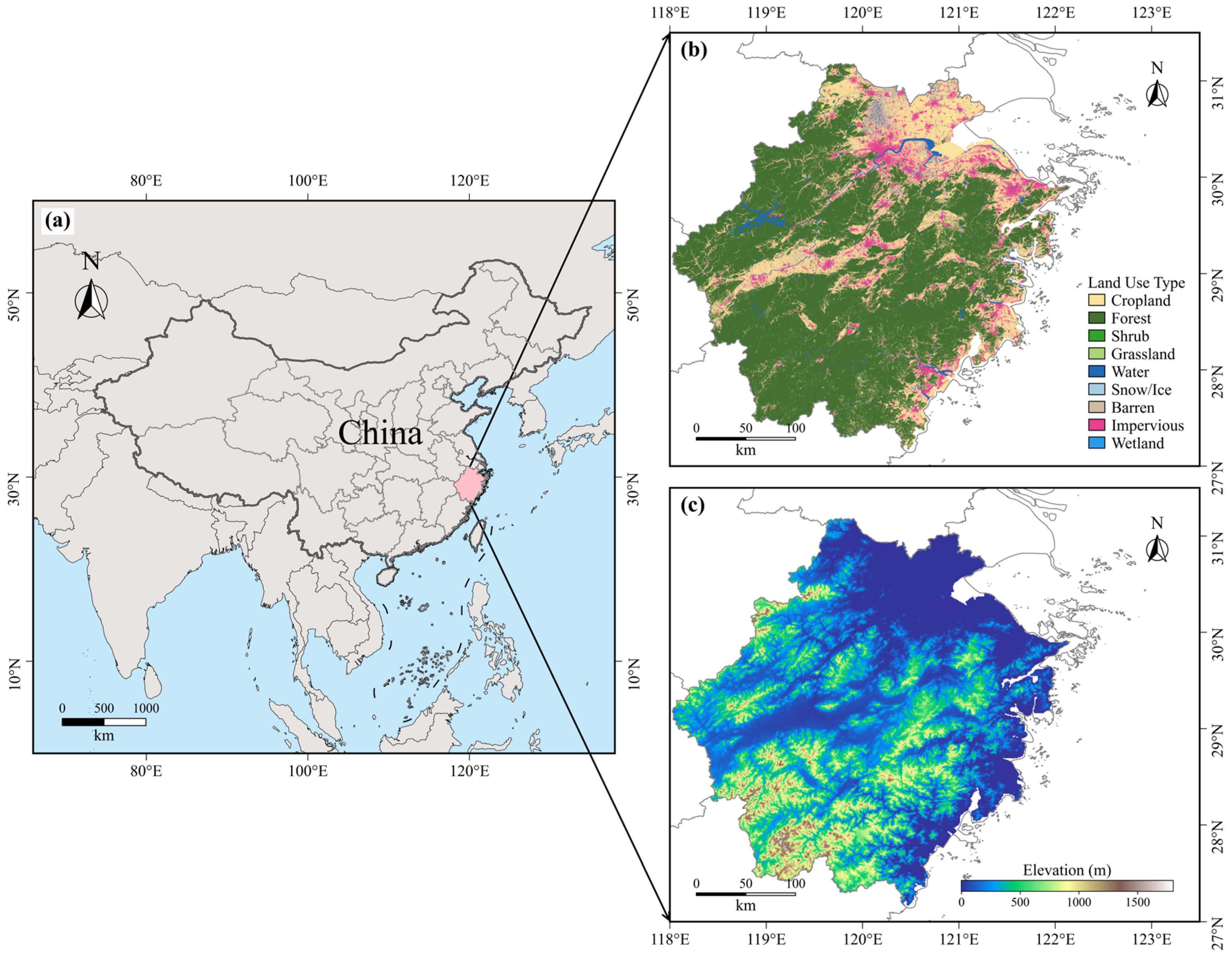
Figure 1. Study area overview: (a) Location of Zhejiang Province; (b) Land use classification map of Zhejiang Province; (c) Digital Elevation Model (DEM) representing the topographic variation.
Remotesensing 17 02865 g001
Figure 2. The flowchart illustrates the overall methodology of this study.
Remotesensing 17 02865 g002
Figure 3. Spatial Distribution of Soil Conservation Services in Zhejiang Province (2001–2020).
Remotesensing 17 02865 g003
Figure 4. Topographic Influences on soil conservation services in Zhejiang Province: (a) aspect, (b) slope, and (c) elevation.
Remotesensing 17 02865 g004
Figure 5. Distribution of Soil Retention Change Trends in Zhejiang Province from 2001 to 2020.
Remotesensing 17 02865 g005
Figure 6. Moran’s I Scatter Plots and Local Autocorrelation Clusters of Soil conservation services in 2001, 2005, 2010, 2015, and 2020.
Remotesensing 17 02865 g006
Figure 7. Spatial Distribution of Potential Environmental and Anthropogenic Factors Affecting Soil Conservation Services in Zhejiang Province.
Remotesensing 17 02865 g007
Figure 8. SHAP-based interpretation of variable contributions to soil conservation services using the XGBoost model. (a) Feature importance ranking based on mean absolute SHAP values. (b) SHAP summary plot showing the direction and magnitude of each variable’s influence, with color representing the feature value.
Remotesensing 17 02865 g008
Figure 9. SHAP dependence plots for the top three variables contributing to the prediction of soil conservation services. Point colors represent the values of the most strongly interacting variable, with blue indicating lower values and red higher values.
Remotesensing 17 02865 g009
Figure 10. SHAP-based interaction analysis among major driving factors affecting soil conservation services. Red indicates high feature values, and blue indicates low feature values.
Remotesensing 17 02865 g010
Figure 11. Heatmaps of SHAP values for the potential driving factors of soil conservation services.
Remotesensing 17 02865 g011
Figure 12. Spatial Distribution of GWR-Estimated Coefficients for Key Influences on Soil Conservation Services in 2001.
Remotesensing 17 02865 g012
Figure 13. Spatial Distribution of GWR-Estimated Coefficients for Key Factors on Soil Conservation Services in 2010.
Remotesensing 17 02865 g013
Figure 14. Spatial Distribution of GWR-Estimated Coefficients for Key Factors on Soil Conservation Services in 2020.
Remotesensing 17 02865 g014
Figure 15. Pearson Correlation Heatmap of Driving Factors for Soil Conservation Services.
Remotesensing 17 02865 g015
Figure 16. Comparison of OLS and GWR Model Fitting Performance in 2001, 2010, and 2020: R2 and Residuals.
Remotesensing 17 02865 g016
Table 1. Main dataset.
CategoryPropertiesAbbreviationFormat and Spatial ResolutionTime ResolutionData Source and Description
target variableSoil Conservation ServiceSCSRaster, 1000 m2001, 2005, 2010, 2015, 2020
human activity
factors
population densityPOPRaster, 100 mAnnual, 2001–2020https://www.worldpop.org/ (accessed on 18 April 2025)
gross domestic productGDPRaster, ~1 kmAnnual, 2001–2020http://www.geodata.cn
(accessed on 18 April 2025)
land use/land coverLULCRaster, ~30 mAnnual, 2001–2020CLCD v01 product
nighttime lightNTLRaster, ~1 kmAnnual, 2001–2020DMSP-OLS and VIIRS
natural environment
factors
elevationELERaster, 30 mStatichttps://cmr.earthdata.nasa.gov/ (accessed on 22 April 2025), NASA SRTMGL1_003
slopeSLORaster, 30 mStaticDerived from NASA SRTMGL1_003
aspectASPRaster, 30 mStaticDerived from NASA SRTMGL1_003
soil textureSTEXRaster, ~1 kmStatichttps://openknowledge.fao.org/ (accessed on 18 April 2025)
bulk densityBDRaster, ~1 kmStatichttps://openknowledge.fao.org/ (accessed on 18 April 2025)
available water capacity (awc)AWCRaster, ~1 kmStatichttps://openknowledge.fao.org/ (accessed on 18 April 2025)
drainageDRARaster, ~1 kmStatichttps://openknowledge.fao.org/ (accessed on 18 April 2025)
root depthRDRaster, ~1 kmStatichttps://openknowledge.fao.org/ (accessed on 18 April 2025)
fao90/phase1FAO90, Phase1Raster, ~1 kmStatichttps://openknowledge.fao.org/ (accessed on 18 April 2025), fao90 represents soil type
climate factorsprecipitationPRERaster, ~1 kmAnnual, 2001–2020http://www.geodata.cn (accessed on 20 April 2025)
temperatureTEMRaster, ~1 kmAnnual, 2001–2020http://www.geodata.cn (accessed on 20 April 2025)
maximum ndviNDVIRaster, 250 mAnnual, 2001–2020MODIS MOD13Q1
solar radiationRADRaster, ~4 kmAnnual, 2001–2020TERRACLIMATE
Table 2. Total Amount and Percentage of Soil Conservation Services in Each City of Zhejiang Province from 2001 to 2020 (Unit: 1000 tons).
20012005201020152020
CitySumPercentSumPercentSumPercentSumPercentSumPercent
Quzhou1349.880.09641186.810.08972162.390.10662054.40.11041532.690.1103
Jinihua983.620.0703929.20.07031450.020.07151286.220.06911012.890.0729
Shaoxing506.440.0362471.960.0357669.670.033613.710.033517.520.0372
Hangzhou1786.60.12761509.740.11412663.660.13132744.450.14752330.110.1677
Lishui5203.560.37174976.350.37637658.710.37766812.20.36614729.760.3404
Taizhou1166.980.08341175.520.08891604.50.07911409.690.07581089.420.0784
Huzhou259.640.0185202.10.0153319.720.0158375.340.0202347.090.025
Jiaxing2.60.00022.010.00022.690.00013.190.00023.240.0002
Wenzhou2149.230.15352214.910.16752990.220.14742620.070.14081719.330.1237
Ningbo475.750.034451.950.0342590.590.0291519.540.0279454.980.0327
Zhoushan0000000011.750.0008
Note: The value for Zhoushan in 2001–2015 is 0 due to the unavailability of valid input data. The value in 2020 represents the first year with retrievable data for this city.
Disclaimer/Publisher’s Note: The statements, opinions and data contained in all publications are solely those of the individual author(s) and contributor(s) and not of MDPI and/or the editor(s). MDPI and/or the editor(s) disclaim responsibility for any injury to people or property resulting from any ideas, methods, instructions or products referred to in the content.