CFDC: A Spatiotemporal Change Detection Framework for Mapping Tree Planting Program Scenarios Using Landsat Time Series Images

Abstract

Artificial afforestation plays a critical role in ecological restoration, but its implementation involves multiple strategies—such as new afforestation, densification, and replacement afforestation. Long-term spatial and temporal identification of these tree planting program scenarios (TPPSs) is key to evaluating ecological restoration policies, yet existing pixel-based time series change detection methods still face challenges in discriminating these patterns on a large scale. To address these challenges, we propose CFDC, the first framework that synergistically integrates Continuous Change Detection (CCD) for temporal spectral trajectories and Focal Context (FC) analysis for spatial neighborhood context. A Spatiotemporal Coupling Index (STCI) is proposed to abstractly summarize the two modules, and a rule-based model classifies TPPSs by their unique temporal–spatial signatures. Implemented on Google Earth Engine (GEE) for Bayi District, Tibet, CFDC delivered overall accuracies of 76.0–82.5% from 2007 to 2022, with user’s accuracies for all TPPS types exceeding 75% in most years. Detected TPPS timelines coincide with documented ecological restoration projects within a ±1-year tolerance. Overall, CFDC offers a novel mechanism that fuses spatiotemporal features to effectively distinguish new afforestation, densification, and replacement afforestation scenarios, addressing the limitations of previous methods and enabling more accurate and scalable TPPS monitoring, thereby supporting scalable artificial forest management and ecological restoration planning.

1. Introduction

Afforestation and reforestation play vital roles in mitigating climate change, enhancing ecosystem services, and meeting carbon neutrality targets [1,2,3]. In recent decades, large-scale ecological restoration programs, particularly in developing countries, have been implemented for degraded landscapes. These initiatives have resulted in various afforestation patterns, referred to as tree planting program scenarios (TPPSs), including:

• New afforestation: new forest establishment on previously non-forested lands.
• Densification: increasing tree density in sparsely wooded areas.
• Replacement afforestation: replacing existing forests with alternative species or management practices.

Effectively distinguishing between various afforestation scenarios, while also tracking their spatial and temporal changes, is essential for evaluating ecological outcomes, improving forest management strategies, and assessing restoration policy effectiveness. However, traditional field-based methods and historical records remain limited in scale and efficiency. They are often costly, time-consuming, and constrained by difficult terrain or inaccessible locations, hindering adequate data acquisition for timely, large-area monitoring [3]. Meanwhile, as an important practitioner of global ecological restoration, China has carried out multiple national-level ecological restoration projects, such as the Grain for Green Program, the Three-North Shelter Forest Program, and the Natural Forest Protection Project [4]. These national programs have generated strong demand for accurate, large-area monitoring tools to support policy evaluation, ecological assessment, and adaptive management.

With its ability to capture large-scale, long-term, and multi-dimensional information, remote sensing has become an essential approach for the identification and monitoring of artificial forests. A range of methods have been developed to utilize spectral, temporal, and structural features. Common methods can be broadly categorized into the following four types: (1) Supervised classification based on spectral or structural features. This approach relies on spectral reflectance, vegetation indices, and textural features extracted from multispectral or hyperspectral imagery [3,4,5]. These features are typically input into traditional classifiers such as Support Vector Machines (SVM) or Random Forests (RF) [1,2,3], etc., to differentiate [6,7,8] artificial forests from other tree species. However, the classification performance is often highly sensitive to the selection and quality of input features. (2) Phenology-based approaches. These methods exploit seasonal changes in vegetation growth to enhance classification accuracy [9]. By analyzing vegetation indices during key phenological stages, researchers can identify species-specific or plantation-specific spectral signatures, supporting more detailed artificial forest type classification [3] and mapping [6,9,10]. (3) Deep learning-based methods. Recent advances in deep learning have provided powerful tools for artificial forest classification. Models such as Convolutional Neural Networks (CNNs) [11,12,13,14,15] and Transformers [9] can automatically learn complex spatial and contextual features from high-resolution images, significantly reducing the need for manual feature engineering. (4) An integrated approach. Integrating multiple methods often yields better performance. Combining spectral and phenological information [9] enhances artificial forest classification accuracy, while incorporating structural features into deep learning [16,17] workflows improves model generalization and efficiency.

Despite these advances, existing approaches often suffer from dependence on high-quality training datasets and limited temporal depth. Time series-based change detection algorithms have currently become effective tools for characterizing forest dynamics. Methods such as Landsat-based Detection of Trends in Disturbance and Recovery (LandTrendr) [18], and Breaks For Additive Season and Trend (BFAST) [19,20], Continuous Change Detection and Classification (CCDC), and CCD [21,22] are widely used to identify gradual or abrupt changes in forest cover, enabling the monitoring of afforestation processes and forest degradation and disturbances [23,24,25]. In China’s ecologically sensitive areas and key forest regions, including the Qinghai-Tibet Plateau, Loess Plateau, Inner Mongolia, and the Daxing’an Mountains, these methods have been extensively applied to identify mining activities, quantify their impacts on vegetation cover, and detect vegetation disturbance and restoration trends [26,27,28,29,30].

LandTrendr [18,31] segments annual composite Landsat data into linear pieces to capture abrupt changes and long-term trends. BFAST [19] identifies change points by decomposing time series data into trend, seasonal, and residual components, though it cannot detect recurring disturbances [32]. CCD, in contrast, uses all clear observations from Landsat time series data and employs a harmonic fitting model with sine and cosine functions to model spectral time series [33,34]. This approach provides higher precision and stability for detecting subtle changes. CCD can detect breakpoints indicating significant land cover changes and dynamically adjust its model to accommodate new observations [35]. Previous studies have systematically compared and validated widely used forest disturbance monitoring algorithms in China. These comparisons revealed that CCD achieved the highest accuracy for monitoring forestation among different forest disturbance types [35].

However, CCD is insufficient for distinguishing specific tree planting program scenarios (TPPSs). This limitation arises because CCD primarily focuses on spectral changes at the pixel level, without incorporating spatial context or neighborhood information—factors that are critical for accurately differentiating between TPPS types. For example, both new afforestation and densification may exhibit similar patterns of positive vegetation growth, but they differ in spatial configuration; new afforestation typically occurs along forest margins adjacent to non-forest areas, while densification takes place within existing forest stands. Similarly, replacement afforestation often presents as a cycle of forest loss followed by regrowth, which may be misinterpreted by pixel-based change detection algorithms. As a result, relying solely on pixel-level spectral trajectories can lead to ambiguity and misclassification, limiting the effectiveness of CCD in TPPS recognition tasks. Therefore, there is a pressing need to integrate spectral, temporal, and spatial contextual information for more accurate and robust TPPS identification.

To overcome the limitations of pixel-based change detection in distinguishing TPPSs, we propose a novel framework—CFDC—that integrates Continuous Change Detection (CCD) with Focal Context (FC) analysis to incorporate both temporal and spatial contextual information. CFDC is built upon the CCD algorithm and enhances its classification capability by introducing neighborhood-level spatial analysis, allowing for the effective separation of new afforestation, densification, and replacement afforestation. Additionally, we integrated spatiotemporal features into a Spatiotemporal Coupling Index (STCI), which operates within a cloud-computing environment to facilitate regional-scale applications. This approach enhances the generalizability of the CFDC framework, making it applicable to ecologically vulnerable and sensitive areas that have undergone tree planting programs. The main objectives of this study are as follows: (1) construct a spatiotemporal coupling module by integrating CCD-based spectral time series analysis with Focal Context analysis to capture both temporal dynamics and spatial neighborhood patterns; (2) develop a classification model based on the distinct temporal and spatial characteristics of TPPSs to identify their occurrence time and spatial distribution; and (3) apply and validate the proposed CFDC framework in a representative ecological restoration region to assess its effectiveness and classification accuracy over multiple years. The proposed framework aims to support scalable, long-term TPPS monitoring and provide decision-making tools for artificial forest management and restoration assessment.

2. Study Area and Data

2.1. Study Area

Bayi District, located in Nyingchi City in southeastern Tibet, was selected as the study area. It lies between 29°21′ and 30°15′N and 93°27′ and 95°17′E, at the confluence of the Yarlung Zangbo River and the Nyang River (Figure 1a). This region encompasses alluvial plains and adjacent valley slopes within the Yarlung Zangbo River Basin, an ecologically fragile zone that has long experienced wetland degradation and desertification. In response, large-scale ecological interventions have been implemented. Specifically, from 2008 to 2014, the Tibet Ecological Security Barrier Protection and Construction Project launched a series of afforestation and wetland restoration programs across southeastern Tibet, including Bayi. More recently, the Major Ecological Protection and Restoration Project Plan for the Qinghai-Tibet Plateau Ecological Barrier Zone (2021–2035) has further reinforced restoration efforts through long-term afforestation, species replacement, and water conservation engineering. Restoration activities (Figure 1b) such as afforestation, densification, and replacement afforestation in Bayi primarily target riparian zones and surrounding slopes, with plantations composed of high-altitude pine species (Pinus spp.), lhasa spruce (Picea likiangensis var. linzhiensis), and walnut (Juglans regia), which are well adapted to local conditions. The dual occurrence of ecosystem degradation and human-led ecological intervention makes Bayi District an ideal natural laboratory for remote sensing-based studies aiming to distinguish between new afforestation, densification, and replacement afforestation scenarios.

2.2. Landsat Data and Preprocessing

In this study, we utilized Landsat surface reflectance imagery acquired between 2003 and 2022 (Figure 2a). All imagery was obtained from the USGS/NASA Landsat Collection 2, Tier 1 archive, which provides Level 2 atmospherically corrected surface reflectance products with a spatial resolution of 30 meters and a nominal 16-day revisit interval. We implemented terrain correction using the SCS+C model with the 30 m SRTM DEM in Google Earth Engine to adjust for solar zenith, azimuth, slope, and aspect effects, especially for forested mountainous regions. For missing Landsat data, we queried existing scenes within the target date range and region, substituting gaps with the closest available dates in the same year or adjacent years, and merged these into a chronologically sorted image collection. Additionally, the CCD algorithm used in this study inherently includes the cloud-masking routine FMask to handle residual clouds.

2.3. Artificial Forest Mask Data

To extract the distribution of artificial forests, we first constructed an artificial forest mask by excluding non-forest and natural forest areas based on the global 30-meter resolution dataset of artificial and natural forests derived from Landsat imagery (1985–2021). Subsequently, artificial forest mask was validated referencing historical high-resolution imagery available in Google Earth Pro. To further improve classification accuracy and reduce potential misclassification, the artificial forest mask was refined using the China 30-meter annual land cover dataset spanning 1990–2022 (

Table 1. Used data list related to artificial forest mask.

Data Type	Period	Spatial Resolution	Data Source
China 30 m Annual Land Cover Data	1990–2022	30 m	[36]
Global 30 m Forest Distribution Data	1985–2021	30 m	[37]

).

2.4. Sample Data

Reference samples for different TPPSs including new afforestation, densification, and replacement afforestation, were collected through a combination of field surveys and visual interpretation of historical high-resolution imagery in Google Earth Pro. Sample collection was conducted for four target years: 2007, 2012, 2017, and 2022 (Figure 1c–f). Field surveys were primarily carried out in accessible forested areas of Bayi District, ensuring coverage across representative landscape types and planting patterns. Complementary samples were derived by visually interpreting temporal changes in canopy cover and land use using time-stamped imagery in Google Earth Pro. Each TPPS type was defined based on observable temporal and spatial characteristics mentioned in introduction part. To ensure consistency and reduce labeling bias, all samples were cross validated by at least two independent analysts. A stratified sampling approach was adopted to maintain balanced representation across classes and years and used for accuracy assessment.

3. Methods

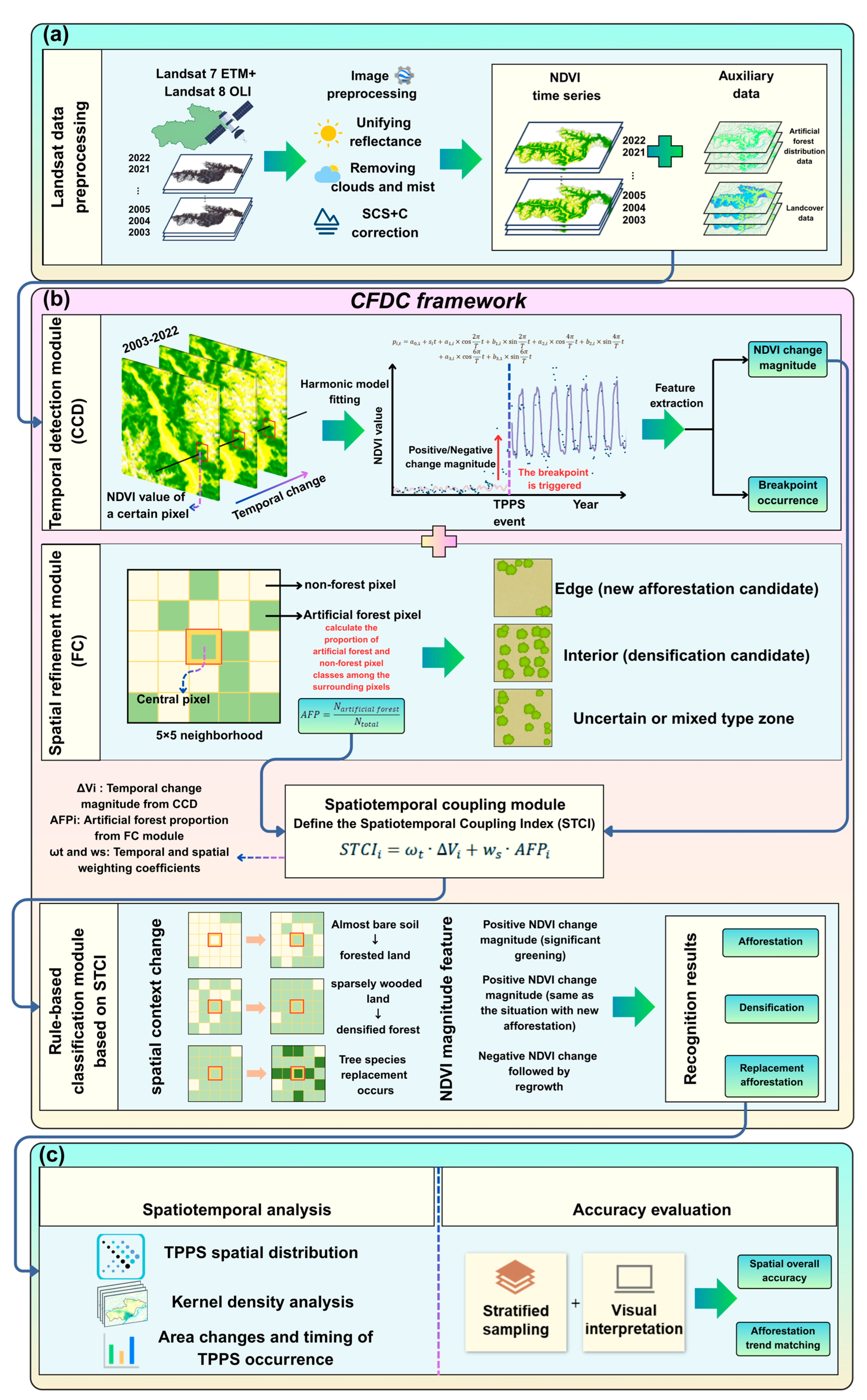
The CFDC (Figure 2b) consists of two core components: (1) a spatiotemporal information extraction module based on the integration of Continuous Change Detection (CCD) and Focal Context (FC) analysis results, and (2) a rule-based classification model designed to discriminate TPPS types based on their distinct temporal and spatial signatures. It can be divided into three main steps:

First, pixel-level NDVI time series trajectories and corresponding spatial neighborhood change indices are extracted by integrating Continuous Change Detection (CCD) with Focal Context (FC) analysis. This step enables the capture of temporally explicit spectral changes alongside their spatial context, forming the basis for spatiotemporal association. Second, a rule-based classification model was constructed based on the previously derived CCD and FC results, using the Spatiotemporal Coupling Index (STCI), which integrates distinct temporal and spatial characteristics of different TPPS types. This model enables accurate identification of both the occurrence time and spatial distribution of various afforestation scenarios. Finally, the proposed method is applied to a representative case study area, where spatiotemporal dynamics of TPPS are analyzed to evaluate the model’s effectiveness and robustness.

3.1. Spatial-Temporal Characteristics of TPPS

Tree planting program scenarios (TPPS) are associated with distinct patterns of landscape transformation. These scenarios differ not only in the magnitude and trajectory of vegetation change over time, but also in their spatial configuration within the surrounding forest context. Such differences are not random but rather reflect the underlying planting strategies and ecological processes unique to each scenario. By analyzing both the temporal sequence of vegetation dynamics and the spatial relationships with adjacent land cover, it is possible to establish discriminative features that support accurate scenario classification. These spatiotemporal characteristics serve as the foundation for constructing a rule-based identification model, and are summarized as follows:

• New afforestation (Figure 3a) is identified by a rapid increase in Normalized Difference Vegetation Index (NDVI) values from near-zero levels, typically occurring within 1–3 years. This sharp change generates a clear breakpoint in the NDVI trajectory, indicating the initial establishment of artificial forests. Before this change, the surrounding pixels predominantly belong to non-forest classes (e.g., bare soil).

• Densification (Figure 3b) also shows a rapid NDVI increase and a detectable breakpoint, similar to new afforestation. However, its spatial context differs; the affected pixels are embedded within existing forest cover, reflecting increases in stand density or underplanting activities rather than expansion into previously non-forested areas.
• Replacement afforestation (Figure 3c) is characterized by a sharp decline in NDVI due to forest clearance or species replacement, followed by a gradual recovery with a distinct NDVI curve. In this case, both pre- and post-change neighborhoods consist of artificial forest, indicating forest management. Our definition of “decline followed by regrowth” is as follows:
• Initial Stable NDVI: The NDVI value of the forest remains a periodic stable fluctuation before the replacement event.
• Sharp Decline: The NDVI decreases significantly in the year of the replacement event.
• Regrowth and Stabilization: As new trees establish, the NDVI begins to rise, ultimately reaching new long-term stable cyclical fluctuation.

3.2. Construction of Spatiotemporal Coupling Module

3.2.1. Temporal Detection Module: Continuous Change Detection (CCD)

The CCD fits long-term Landsat-based NDVI time series using a harmonic model. It detects multiple types of changes including seasonal, gradual, and abrupt events by identifying structural breakpoints in the fitted NDVI trajectories [38]. Breakpoints are triggered when predicted NDVI values deviate from actual observations over a sequence of dates. We defined a breakpoint in the NDVI time series when six consecutive Landsat observations deviated from the model prediction by more than two times the root mean square error (RMSE), in order to reduce the likelihood of false change detection. The NDVI time series is modeled using a harmonic regression function as follows [21,39]:

$$p_{i,t}=a_{0,1}+s_{i}t+a_{1,i}\times \cos {\displaystyle \frac{2\pi }{T}}t+b_{1,i}\times \sin {\displaystyle \frac{2\pi }{T}}t+a_{2,i}\times \cos {\displaystyle \frac{4\pi }{T}}t+b_{2,i}\times \sin {\displaystyle \frac{4\pi }{T}}t+a_{3,i}\times \cos {\displaystyle \frac{6\pi }{T}}t+b_{3,1}\times \sin {\displaystyle \frac{6\pi }{T}}t$$

(1)

where

$p_{i,t}$: predicted NDVI value for pixel on Julian date

$t$$T$: number of days in a year

$a_0,s,a_n,b_n$: model coefficients representing intercept, trend, and seasonal components

The CCD algorithm was chosen as the foundation of the CFDC framework because it can accurately capture subtle changes and seasonal dynamics in the NDVI time series through harmonic fitting. CCD can precisely identify breakpoints in the NDVI trajectory. Moreover, in the case of replacement afforestation, the NDVI waveform before and after the change is distinctly different due to differences in tree species, and during the change period, NDVI typically shows a decline followed by a recovery. This capability, which is difficult for other methods to achieve, gives CCD a significant advantage in distinguishing afforestation scenarios and provides a more precise tool for ecological restoration monitoring.

In the CCD algorithm, we have adopted the default parameter settings to balance sensitivity and specificity in change detection. Specifically, the parameter minObservations is set to 6, requiring a minimum of six observations to flag a change. This setting follows the general rule of thumb in time series analysis to ensure that detected changes are not due to random fluctuations but represent actual significant transitions. The chiSquareProbability is set to 0.99, corresponding to a 99% confidence level, which reduces the likelihood of false positives by detecting only changes that are highly unlikely under the null hypothesis (no change). Additionally, the minNumOfYearsScaler is set to 1.3, ensuring that the algorithm does not detect changes over too short a period, which might be indicative of noise rather than a true signal. The CCD module within the CFDC framework plays two critical roles by continuously analyzing Landsat-derived NDVI time series:

• It extracts the breakpoint timing, capturing the moment when a significant vegetation change occurs.
• It determines the direction and magnitude of NDVI change, which helps infer the nature of the TPPS.

These temporal features form the foundation of the CFDC model for identifying TPPSs across multiple years and large spatial extents.

3.2.2. Spatial Refinement Module: Focal Context (FC)-Based Neighborhood Context

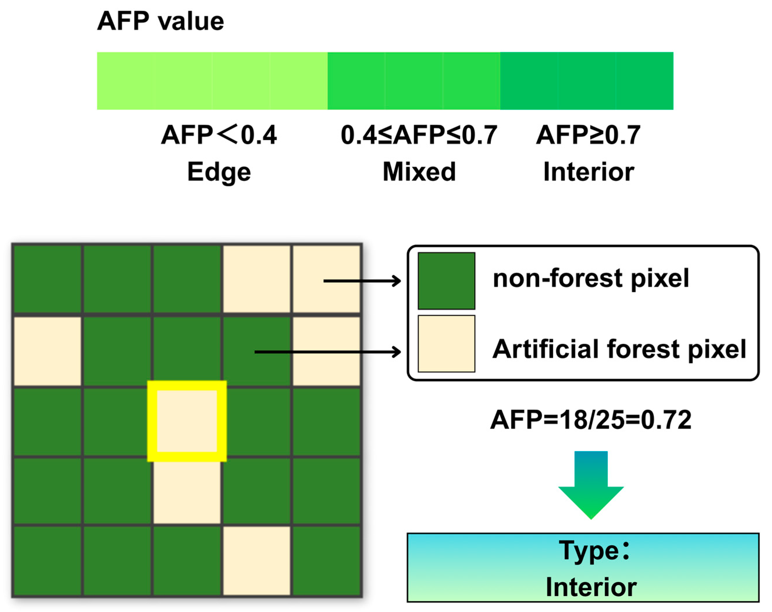
Focal context analysis was employed to quantify the spatial neighborhood composition of the target pixel that was detected as changing by temporal detection module (Figure 4). To select an optimal window size, we evaluated 3 × 3, 5 × 5, 7 × 7, 9 × 9, 11 × 11, and 13 × 13-pixel neighborhoods. The coefficient of variation (CV) of the artificial forest proportion (AFP) among 200 random samples peaks at windows = 5 × 5, indicating an “edge-interior”-sensitive metric. The 5 × 5 window (150 m × 150 m) represents an elbow point where further increases or decreases in size yield diminishing sensitivity and begin to blur meaningful AFP patterns. This scale is consistent with the average width of riparian planting belts observed in the study area. Specifically, the artificial forest proportion (AFP) was defined as

$$AFP={\displaystyle \frac{N_{artificialforest}}{N_{total}}}$$

(2)

where:

$N_{artificial forest}$ is the number of artificial forest-class pixels within the 5×5 neighborhood; $N_{total}$ is the total number of pixels in the neighborhood; and $AFP$ ranges from 0 to 1, representing the degree of forest dominance in the local context.

Based on this proportion, the spatial context of each pixel was characterized as follows:

• Edge (new afforestation candidate): e.g., AFP < 0.4
• Interior (densification candidate): e.g., AFP ≥ 0.7
• Uncertain or mixed type zone: e.g., 0.4 ≤ AFP < 0.7

Metrics such as patch density (PD), edge density (ED), and forest area density (FAD) are commonly used to assess forest landscape fragmentation. FAD has been employed in previous studies to differentiate continuous forests from forest patches by setting thresholds and calculating values at multiple window scales [40,41,42,43]. The principle of AFP is similar to FAD, and it has been used to assess the spatial configuration of afforestation patches in our study area.

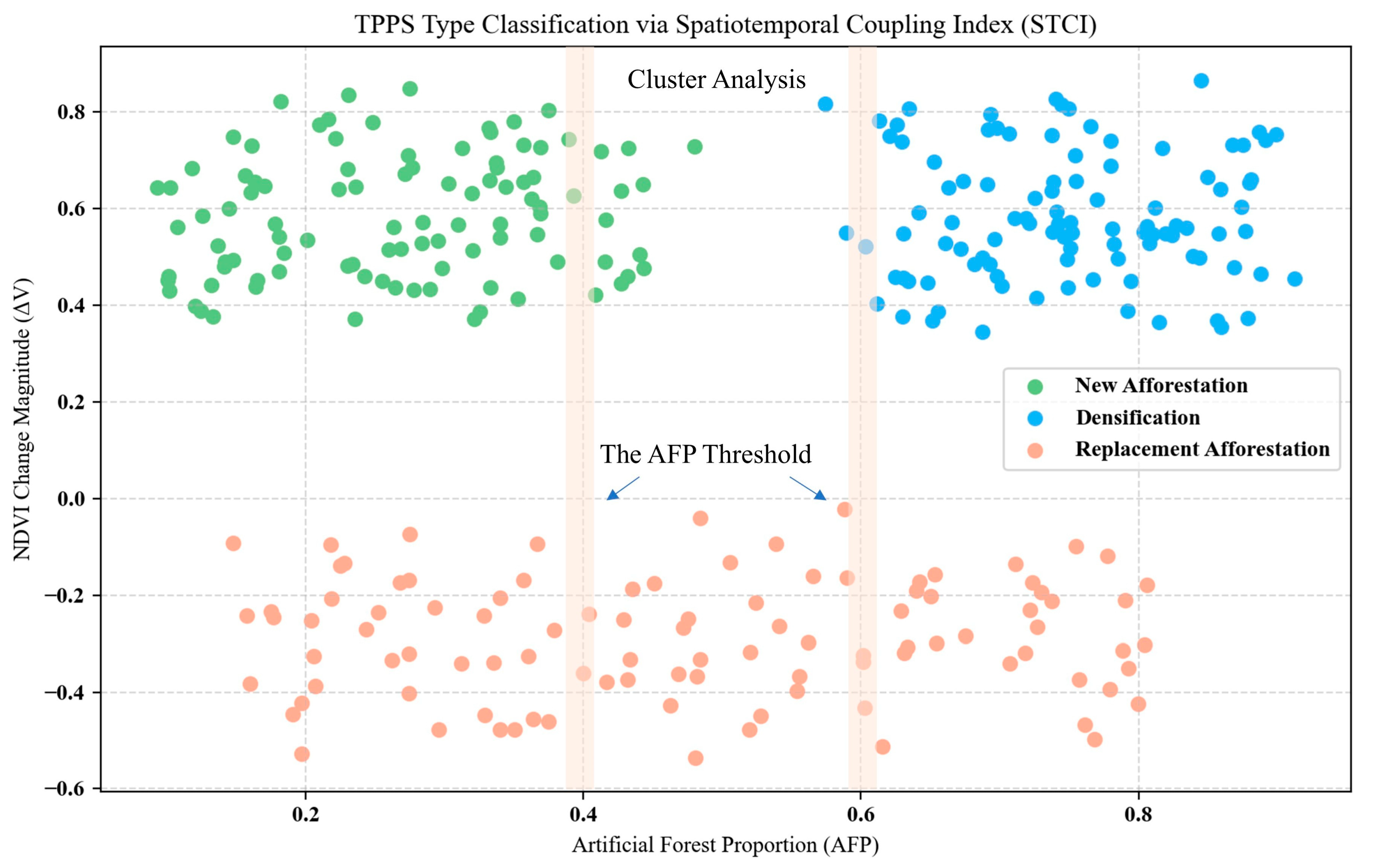
In this study, the unsupervised k-means clustering approach revealed natural breakpoints in the AFP distribution, providing a scientific basis for classification. The low and high AFP thresholds in our study area were determined to be 0.58 and 0.90, respectively. For application to other ecological regions, the AFP thresholds should be recalibrated based on new validation samples and the actual spatial density patterns of plantations in those landscapes.

3.2.3. Spatiotemporal Coupling Module

To abstractly summarize the integration of temporal and spatial information, we designed a spatiotemporal coupling module that synthesizes outputs from both the CCD-based temporal detection and FC-based spatial context analysis. Specifically, for each pixel $i$, we define the Spatiotemporal Coupling Index (STCI) as follows:

$$STC{I}_i={\omega }_t·\Delta V_i+w_s·AF{P}_i$$

(3)

where

$\Delta V_i$ is the temporal change magnitude, derived from the CCD module, representing the maximum positive or negative deviation in NDVI within the identified breakpoint period. This reflects the intensity and direction of vegetation change. $AF{P}_i$ is the artificial forest proportion, calculated from the 5 × 5 window in the FC module, representing the proportion of artificial forest pixels within the neighborhood and characterizing the local spatial configuration of the change. ${\omega }_t$ and $w_s$ are weighting coefficients for temporal and spatial contributions, respectively. These can be set equally (e.g., 0.5) or optimized based on validation data or sensitivity analysis.

In applying the Spatiotemporal Coupling Index (STCI), appropriate weights for the temporal (${\omega }_t$) and spatial ($w_s$) components must be regionally tuned. We conducted a sensitivity analysis by varying the weights (with ${\omega }_t$ + $w_s$ = 1) and evaluated classification accuracy on validation samples via k-means clustering. The results indicated that ${\omega }_t$ = $w_s$ = 0.5 yielded good performance in our region, offering a balanced representation of temporal dynamics and spatial context. When extending CFDC to other ecologically sensitive regions, a similar grid search procedure should be performed to optimize the ${\omega }_t$/$w_s$ combination for local conditions.

This index reflects both the temporal intensity and spatial setting of the observed change, enabling better characterization of planting patterns, especially for the subtle differences between new afforestation type and densification type. For example, pixels with high $\Delta V$ and low $AFP$ are typically located at the forest and non-forest boundary and are associated with new afforestation, while pixels with high $\Delta V$ and high $AFP$ are more likely to reflect densification within existing forest stands (Figure 5). The STCI serves as an input to the rule-based TPPS classification model.

3.2.4. Rule-Based Discriminative Module Construction

To differentiate among various TPPSs systematically, a rule-based discriminative module was constructed after the Spatiotemporal Coupling Module that leverages distinctive spatiotemporal signatures captured by CCD and FC. These three representative TPPS types exhibit markedly different patterns (

Table 2. The spatiotemporal characteristics and STCI expression of three scenarios.

TPPS Type	Temporal Feature (CCD)	Spatial Feature (FC)	STCI Pattern Expression
New Afforestation	Positive NDVI change magnitude (significant greening)	Adjacent to non-forest areas, primarily at edges	Strong temporal change + edge spatial context
Densification	Positive NDVI change magnitude (same as the situation with new afforestation)	Completely surrounded by existing forest	Strong temporal change + internal spatial context
Replacement	Negative change followed by regrowth	Minimal spatial shift	Strong temporal fluctuation + stable spatial context

) in both temporal dynamics and spatial configuration, which are quantitatively captured through STCI components. New afforestation is characterized by a significant positive NDVI change (strong greening) and a spatial location adjacent to non-forest areas (i.e., artificial forest expansion at the edge). These pixels typically exhibit high temporal magnitude values ($\Delta V$) and low forest proportion ($AFP$), reflecting a “strong temporal characteristics + edge spatial” profile. Densification usually displays the same NDVI increase with new afforestation, but it is within existing forest interiors where the neighborhood is predominantly artificial forest. These areas show high $\Delta V$ and high $AFP$, forming a “strong temporal characteristics + internal spatial” pattern. In addition, replacement afforestation often involves an initial NDVI decrease followed by regrowth. Spatially, such areas tend to remain within artificial forest zones, with little change in $AFP$ before and after the TPPS event. The resulting STCI signals exhibit temporally oscillating patterns, consistent with a “volatile temporal + stable spatial” signature.

3.3. Accuracy Evaluation Method

To evaluate the performance of the proposed CFDC framework in identifying tree TPPSs, both spatial and temporal accuracy assessments were conducted. Spatial accuracy was assessed by comparing the CFDC-derived TPPS classification results with manually interpreted reference samples. High-resolution satellite imagery (e.g., Google Earth or PlanetScope) and field-assisted visual interpretation were used to generate validation polygons representing the three TPPS types. We employed a stratified random sampling strategy based on the area proportion of each class and 200 samples were taken in each validation year, excluding any overlap with previously sampled points to ensure independence. The overall accuracy (OA) was calculated using the following formula:

$$OA={\displaystyle \frac{{{\displaystyle \sum }}_{i=1}^3{C}_i}{N}}\times 100\%$$

(4)

where

$C_i$ corresponds to the correct classification numbers of new afforestation, densification, and replacement afforestation.

Temporal accuracy was assessed by comparing the year-by-year trend of afforestation-related changes detected by CFDC with the documented timeline of ecological restoration programs and major tree planting initiatives over the past several decades. This comparison included land-use change records, official government reports, and previously published studies, allowing us to evaluate the consistency between observed change timing and historically recorded afforestation efforts (considering a delay of ±1 year).

4. Results

The CFDC method generated two main outputs including TPPS spatial distribution and spatiotemporal changes of TPPS from 2003 to 2022.

4.1. TPPS Spatial Distribution

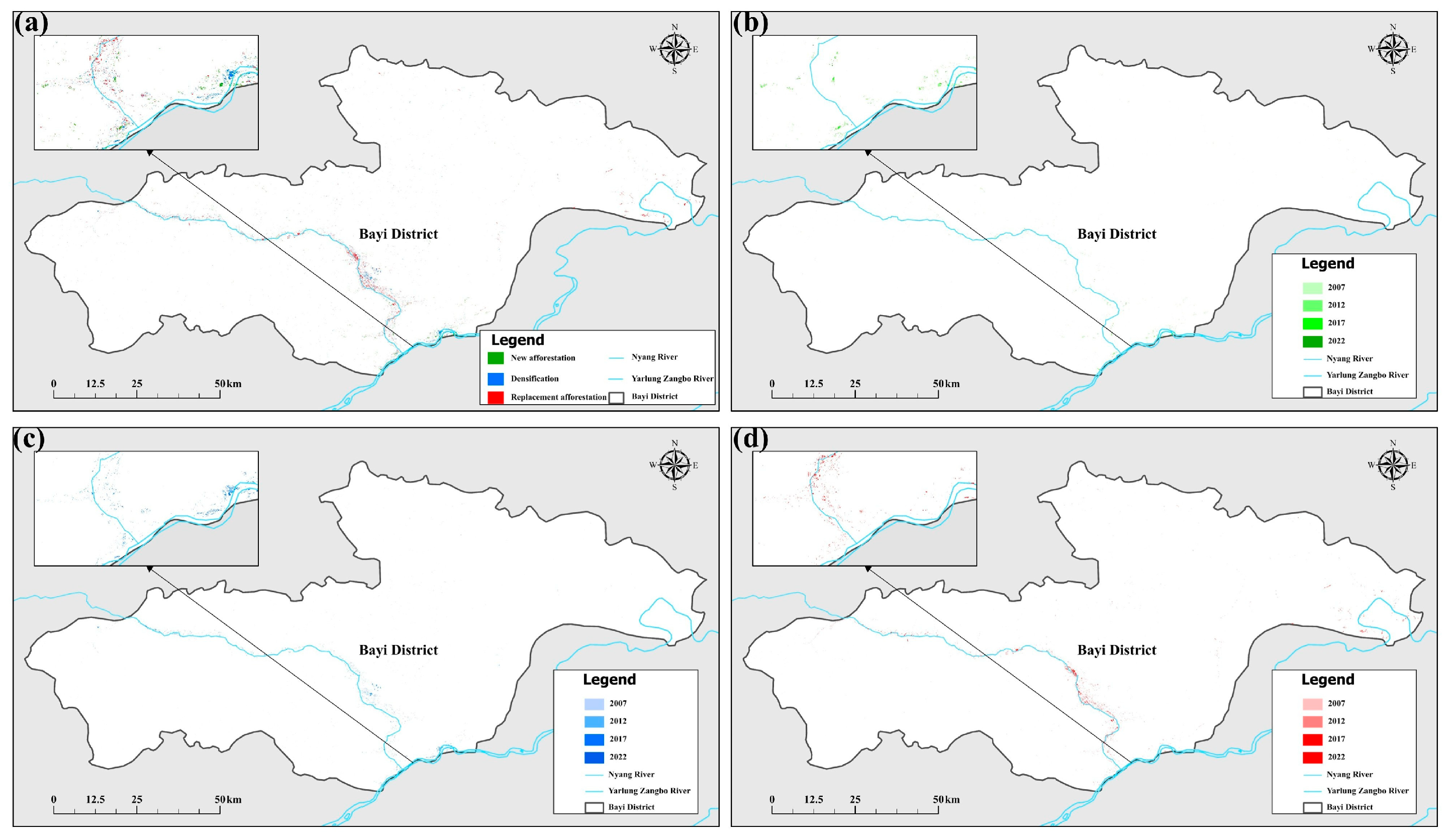
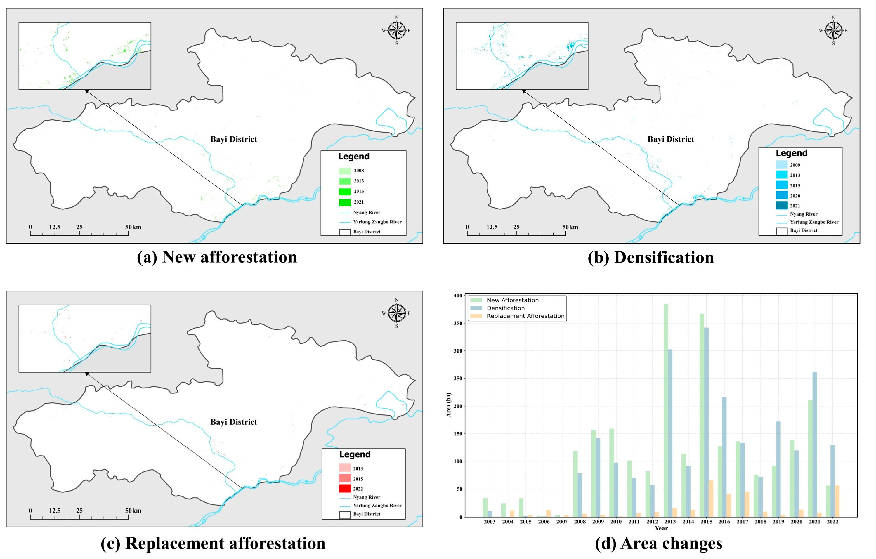
The primary output of CFDC consists of annual per-pixel classification maps that differentiate three TPPSs: new afforestation, densification, and replacement afforestation (Figure 6a–d). These maps were generated at a spatial resolution of 30 meters and provide year-by-year snapshots of afforestation-related land surface changes. By aligning classification with detected breakpoints in NDVI trajectories, the maps reflect interannual structural changes in forest cover associated with human-driven planting activities.

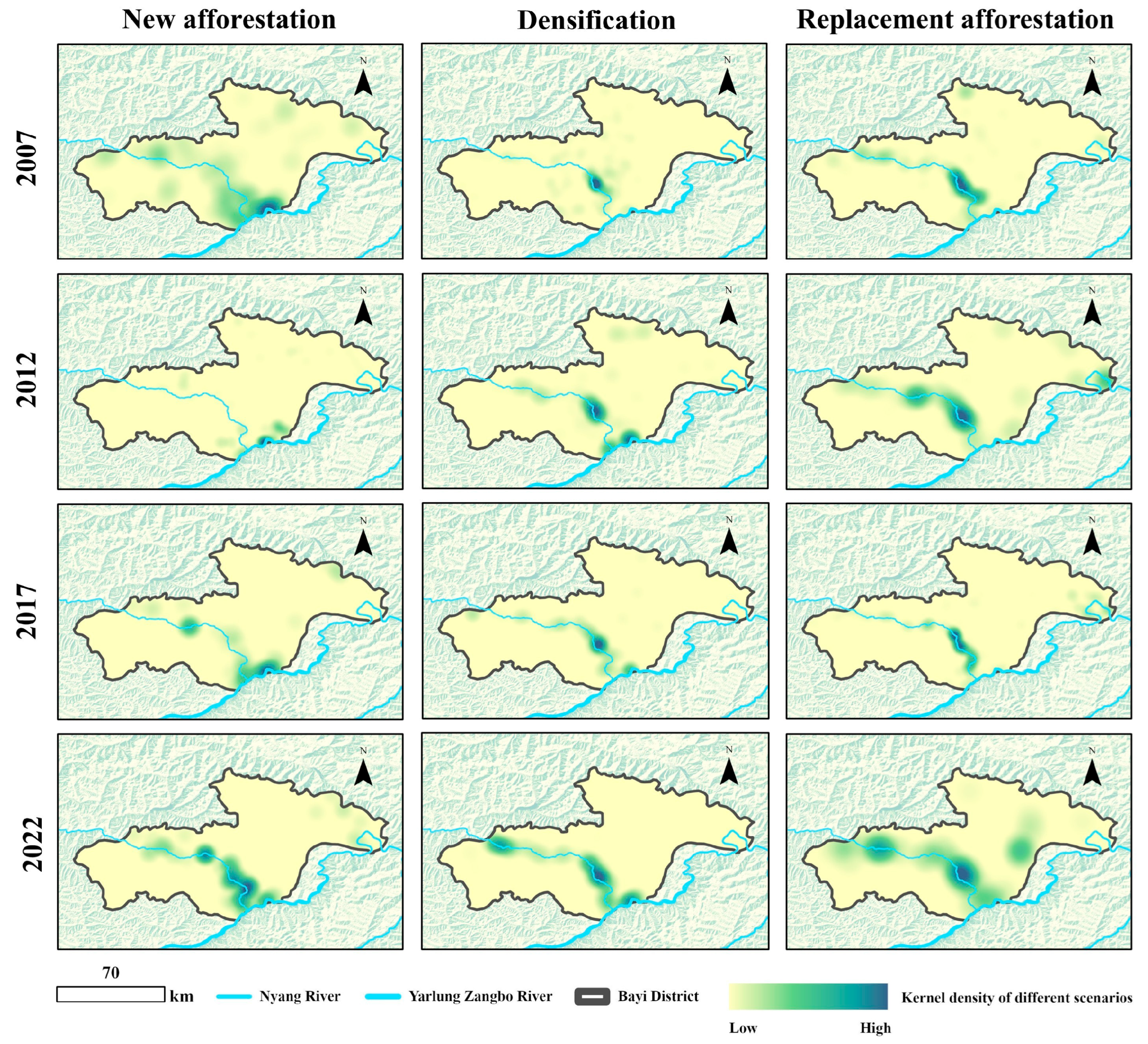
CFDC enables the production of spatial clustering indicators through kernel density analysis of scenario-specific pixels (Figure 7). For each year, 500 random points from each afforestation type were sampled and used to compute density surfaces. These kernel layers reveal landscape-scale distribution tendencies of different TPPS types, such as aggregation near river corridors or settlement areas. The density maps offer a generalized spatial abstraction that complements pixel-level outputs.

4.2. Spatiotemporal Changes of TPPS

CFDC detected the main occurrence years of afforestation activities under three scenarios (Figure 8a–c). New afforestation was mainly observed in 2008, 2013, 2015, and 2021. Densification occurred frequently in 2009, 2013, 2015, 2020, and 2021. Replacement afforestation showed limited activity, with noticeable increases in 2013, 2015, and 2022. Among these, 2013 and 2015 were the most active years, with simultaneous peaks across all three scenarios. At the same time, we also mapped the spatial distribution of timing of occurrence for each TPPS type, revealing its spatial distribution transition, mainly concentrated on both sides of the riverbank.

In addition to identifying the timing of TPPS events, we validated and rectified the distribution results of the TPPSs generated by the CFDC over the study period, conducted a statistical analysis, and plotted the annual changes in area (Figure 8d). The spatial extent of TPPSs exhibited distinct temporal patterns and increasing magnitudes. Overall, new afforestation showed a steady increase in area from 2003 to 2022, reflecting continuous expansion of forested land into previously non-forested regions. The most significant growth was observed in 2013 and 2015, corresponding to regional policy efforts promoting large-scale ecological restoration. Densification areas also increased simultaneously, primarily concentrated within existing forest patches where vegetation structure became denser. This trend indicates ongoing management activities aimed at enhancing forest quality rather than expanding forest extent. In contrast, replacement afforestation displayed more variable dynamics, with notable peaks in certain years that suggest episodes of forest disturbance followed by replanting. The temporal fluctuation in replacement afforestation likely corresponds to cycles of planned harvesting, pest or fire damage, and subsequent restoration interventions.

4.3. Accuracy Evaluation

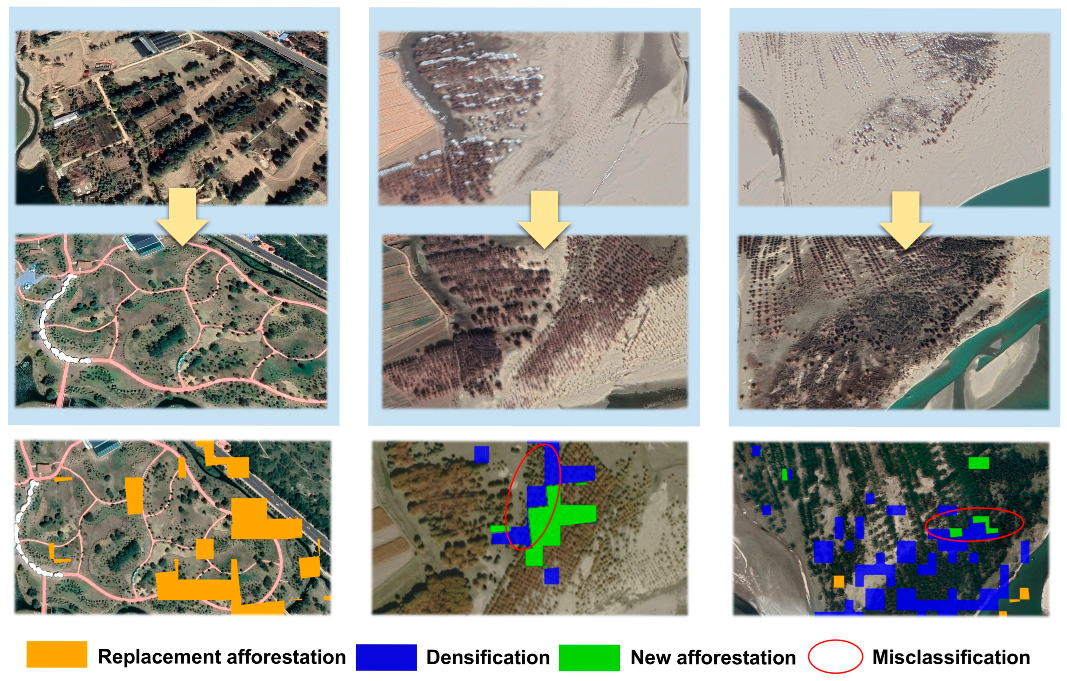
By referencing the NDVI time series generated using the Continuous Change Detection (CCD) algorithm, integrating multiple remote sensing products, and performing visual interpretation using historical imagery from Google Earth Pro (Figure 9), we evaluated the classification performance for multiple validation years. The overall classification accuracies (OAs) were 81.5% in 2007, 81.0% in 2012, 76.0% in 2017, and 82.5% in 2022 (

Table 3. Accuracy evaluation for each year of 2007, 2012, 2017, and 2022.

Validated Year	Overall Accuracy (OA)	User’s Accuracy (UA)
		New Afforestation	Densification	Replacement Afforestation
2007	81.5%	81.1%	80.0%	81.8%
2012	81.0%	78.6%	83.3%	81.1%
2017	76.0%	66.7%	68.2%	80.0%
2022	82.5%	76.7%	82.2%	85.0%
Average	80.25%	75.78%	78.43%	81.98%

), indicating generally stable model performance across time.

In terms of user’s accuracy (UA) (Table 3) for individual TPPS types, New afforestation showed accuracy, with UA values of 81.1% (2007), 78.6% (2012), 66.7% (2017), and 76.7% (2022). Densification had accuracy, with UA values of 80.0%, 83.3%, 68.2%, and 82.2% for the respective years. Replacement afforestation exhibited performance reaching UAs of 81.8%, 81.1%, 80.0%, and 85.0% from 2007 to 2022. Upon calculating the standard deviation for these Overall Accuracy values across the different years, the result was 2.51%. This standard deviation indicates that while there is some variability in the Overall Accuracy for the different TPPS types over the years, the overall precision remains within a manageable range. Additionally, the classification accuracy declined in 2017 mainly due to rapid river level changes that reshaped riparian sandbars and caused significant land-cover alterations. The land cover product used was not responsive enough to these short-term fluvial changes. Some plantations near the river were temporarily submerged during flooding, which compromised the reliability of CCD breakpoint detection.

These results underscore the effectiveness of the spatiotemporal coupling strategy in capturing diverse TPPS types.

5. Discussion

This study presents the CFDC framework, designed to differentiate three major types of tree planting program scenarios (TPPSs): new afforestation, densification, and replacement afforestation. By integrating spatial neighborhood characteristics with temporal spectral dynamics, the method offers an enhanced perspective for detecting annual artificial forest changes, including area changes and spatial distribution. Experimental results demonstrate that CFDC effectively captures the spatiotemporal patterns of TPPS, achieving good overall accuracy. The existing source of misclassification error mainly lies in two aspects: first, the threshold-based division of the $AFP$ still results in ambiguous zones where the boundary and interior areas are not clearly distinguishable. CFDC uses NDVI change magnitude and AFP as the core criteria for distinguishing between TPPSs, and its regulation is effective in the “boundary–interior” binary scenario. However, in some special circumstances, when new afforestation is conducted at the edge of existing clustered artificial forests, the AFP within the window may reach the threshold for forest interior. This can sometimes be confused with the spatial neighborhood characteristics of densification within existing forests, leading to misclassification as densification. At this point, relying on CCD and AFP cannot accurately distinguish between them (Figure 9). Second, the high and low mean values of AFP were divided by cluster analysis and some of the parts between the high and low mean values still belonged to newly added forests or encrypted forests, resulting in misclassification in actual recognition. Third, the breakpoint detection of the CCDC algorithm requires multiple observations over time, which introduces a delay in temporal response.

5.1. Advantages and Disadvantages of CFDC

The CFDC framework offers several notable advantages. Its results align well with both previous research and the documented implementation timeline of the Ecological Security Barrier Plan in Xizang, demonstrating strong consistency with observed trends [44]. In constructing the CFDC framework, we opted for CCD over LandTrendr and BFAST due to its superior ability to process high-frequency Landsat data and capture both short-term fluctuations and long-term trends. Unlike LandTrendr, which relies on annual composites and may overlook short-term changes, CCD directly handles all available observations, providing more detailed temporal information. Compared to BFAST, which is adept at detecting gradual changes but less responsive to short-term variations and unable to detect repeated disturbances, CCD’s harmonic model offers more stable and detailed change detection, serving as a robust foundation for CFDC framework. CFDC also exhibits high transferability, owing to its foundation in the CCD algorithm, which has been successfully applied across diverse forest ecosystems and geographic regions [23,24]. In terms of operational efficiency, CFDC is semi-automated and cloud-based, utilizing the GEE platform to process dense Landsat time series [45] on a per-pixel basis, thus enabling scalable and efficient large-area monitoring with minimal manual intervention. Furthermore, its ability to dynamically update results as new imagery becomes available allows for near real-time tracking of forest changes.

However, CFDC is not without limitations. In areas with complex terrain or heterogeneous land use, spectral confusion may occur due to the similarity between artificial forest plantations and natural vegetation types [46], even when auxiliary datasets such as land cover maps are integrated. Cropland fields with rotationally cultivated crops exhibit NDVI patterns similar to those of afforestation activities, making it difficult to distinguish between the two classes using NDVI and AFP thresholds. This overlap introduces classification errors. Additionally, the long-term and often overlapping nature of afforestation activities poses challenges for precise temporal delineation, especially when transitions between scenarios are gradual. Lastly, the short-term interference sensitivity of the CCD algorithm is exacerbated in regions with frequent land cover changes, such as those experiencing natural disturbances like floods and fires. These events generate a high density of change signals in the time series data, making it difficult to accurately identify each change point. Additionally, inconsistent image acquisition, such as missing or low-quality images during certain periods, can cause the algorithm to miss critical change signals. These further compromise the accuracy of change detection, highlighting the challenges posed by short-term interferences in dynamic landscapes.

5.2. Future Application Prospects of CFDC

To improve classification flexibility and accuracy in complex landscapes, object-oriented classification approaches could be explored in future work. Moreover, spectral similarity among replacement afforestation species poses challenges for conventional spectral methods. Tree growth is further affected by environmental variability and phenological stages, increasing intra-species differences and inter-species overlap. Future research can leverage deep learning methods, such as CNNs [47], which are capable of extracting subtle spectral and textural features for improved species recognition. To address the limitations of CFDC in distinguishing the “ambiguous” TPPSs mentioned earlier, in the future, we will consider using some different methods to solve the problem: (1) Incorporating hyperspectral, LiDAR, and other multi-source data will refine spatial heterogeneity characterization [48]. (2) Introducing a time window sliding strategy to perform breakpoint monitoring within a movable short-term window. (3) Using fuzzy membership degree or probability output to quantify the “mixture degree”. Additionally, diffusion models, which iteratively denoise to produce realistic synthetic samples, could simulate detailed point cloud data for different tree species, improving classification robustness. These innovations will enhance forest resource inventorying and inform evidence-based forest management practices.

6. Conclusions

A novel spatiotemporal change detection framework, CFDC, was introduced for identifying and classifying different tree planting program scenarios (TPPSs), including new afforestation, densification, and replacement afforestation. By integrating temporal spectral trajectories derived from Continuous Change Detection (CCD) with spatial neighborhood analysis through Focal Context (FC), CFDC effectively captures the complex patterns of afforestation-related changes that are often missed by conventional pixel-based approaches. The framework employs a rule-based classification model that leverages both temporal and spatial features to distinguish among TPPS types. To evaluate its performance, we conducted both spatial and temporal accuracy assessments. Spatial validation using visually interpreted reference samples presented user’s accuracy for each TPPS type and overall classification accuracies of 81.5% (2007), 81.0% (2012), 76.0% (2017), and 82.5% (2022). Temporal accuracy, assessed by comparing CFDC-detected change years with historical afforestation records, showed trend consistency with afforestation policies at various stages (considering the possible ±one-year delay in CFDC). These results confirm the robustness and reliability of CFDC in detecting both the location and timing of afforestation changes over extended periods. The framework is scalable and adaptable, making it suitable for large-scale ecological restoration monitoring and forest policy evaluation. Future research will focus on extending the model to incorporate additional spectral indicators and automating the rule-based classification process through machine learning to enhance generalizability in more diverse landscapes.

References

1. Yao, L.; Liu, T.; Qin, J.; Jiang, H.; Yang, L.; Smith, P.; Chen, X.; Zhou, C.; Piao, S. Carbon sequestration potential of tree planting in China. Nat. Commun. 2024, 15, 8398. [Google Scholar] [CrossRef]
2. Kim, J.; Lim, C.-H.; Jo, H.-W.; Lee, W.-K. Phenological classification using deep learning and the sentinel-2 satellite to identify priority afforestation sites in North Korea. Remote Sens. 2021, 13, 2946. [Google Scholar] [CrossRef]
3. Cheng, K.; Su, Y.; Guan, H.; Tao, S.; Ren, Y.; Hu, T.; Ma, K.; Tang, Y.; Guo, Q. Mapping China’s planted forests using high resolution imagery and massive amounts of crowdsourced samples. ISPRS J. Photogramm. Remote Sens. 2023, 196, 356–371. [Google Scholar] [CrossRef]
4. Ding, Z.; Zheng, H.; Liu, Y.; Zeng, S.; Yu, P.; Shi, W.; Tang, X. Spatiotemporal patterns of ecosystem restoration activities and their effects on changes in terrestrial gross primary production in Southwest China. Remote Sens. 2021, 13, 1209. [Google Scholar] [CrossRef]
5. Zhen, J.; Mao, D.; Shen, Z.; Zhao, D.; Xu, Y.; Wang, J.; Jia, M.; Wang, Z.; Ren, C. Performance of xgboost ensemble learning algorithm for mangrove species classification with multisource spaceborne remote sensing data. J. Remote Sens. 2024, 4, 0146. Available online: https://spj.science.org/doi/10.34133/remotesensing.0146 (accessed on 23 June 2025). [CrossRef]
6. Wang, M.; Zheng, Y.; Huang, C.; Meng, R.; Pang, Y.; Jia, W.; Zhou, J.; Huang, Z.; Fang, L.; Zhao, F. Assessing Landsat-8 and Sentinel-2 spectral-temporal features for mapping tree species of northern plantation forests in Heilongjiang Province, China. For. Ecosyst. 2022, 9, 100032. [Google Scholar] [CrossRef]
7. Yang, Y.; Meng, Z.; Zu, J.; Cai, W.; Wang, J.; Su, H.; Yang, J. Fine-scale mangrove species classification based on uav multispectral and hyperspectral remote sensing using machine learning. Remote Sens. 2024, 16, 3093. [Google Scholar] [CrossRef]
8. Xiao, Y.; Wang, Q.; Zhang, H.K. Global Natural and Planted Forests Mapping at Fine Spatial Resolution of 30 m. J. Remote Sens. 2024, 4, 0204. Available online: https://spj.science.org/doi/10.34133/remotesensing.0204 (accessed on 23 June 2025). [CrossRef]
9. Huang, Z.; Zhong, L.; Zhao, F.; Wu, J.; Tang, H.; Lv, Z.; Xu, B.; Zhou, L.; Sun, R.; Meng, R. A spectral-temporal constrained deep learning method for tree species mapping of plantation forests using time series Sentinel-2 imagery. ISPRS J. Photogramm. Remote Sens. 2023, 204, 397–420. [Google Scholar] [CrossRef]
10. Liang, X.; Chen, J.; Gong, W.; Puttonen, E.; Wang, Y. Influence of data and methods on high-resolution imagery-based tree species recognition considering phenology: The case of temperate forests. Remote Sens. Environ. 2025, 323, 114654. [Google Scholar] [CrossRef]
11. Onishi, M.; Ise, T. Explainable identification and mapping of trees using UAV RGB image and deep learning. Sci. Rep. 2021, 11, 903. [Google Scholar] [CrossRef]
12. Korznikov, K.A.; Kislov, D.E.; Altman, J.; Doležal, J.; Vozmishcheva, A.S.; Krestov, P.V. Using U-Net-like deep convolutional neural networks for precise tree recognition in very high resolution RGB (red, green, blue) satellite images. Forests 2021, 12, 66. [Google Scholar] [CrossRef]
13. Fu, M.; Lu, C.; Mao, Y.; Zhang, X.; Wu, Y.; Luo, H.; Liu, Z.; Li, W.; Ou, G. An efficient and accurate deep learning method for tree species classification that integrates depthwise separable convolution and dilated convolution using hyperspectral data. Int. J. Digital Earth 2024, 17, 2307999. [Google Scholar] [CrossRef]
14. Wu, J.; Chen, L.; Wang, J.; Li, Y.; Chen, E.; Zhang, X. A novel framework combining band selection algorithm and improved 3D prototypical network for tree species classification using airborne hyperspectral images. Comput. Electron. Agric. 2024, 219, 108813. [Google Scholar] [CrossRef]
15. Luo, M.; Tian, Y.; Zhang, S.; Huang, L.; Wang, H.; Liu, Z.; Yang, L. Individual tree detection in coal mine afforestation area based on improved Faster RCNN in UAV RGB images. Remote Sens. 2022, 14, 5545. [Google Scholar] [CrossRef]
16. Henrich, J.; van Delden, J.; Seidel, D.; Kneib, T.; Ecker, A.S. TreeLearn: A deep learning method for segmenting individual trees from ground-based LiDAR forest point clouds. Ecol. Inf. 2024, 84, 102888. [Google Scholar] [CrossRef]
17. Shen, X.; Huang, Q.; Wang, X.; Li, J.; Xi, B. A deep learning-based method for extracting standing wood feature parameters from terrestrial laser scanning point clouds of artificially planted forest. Remote Sens. 2022, 14, 3842. [Google Scholar] [CrossRef]
18. Kennedy, R.E.; Yang, Z.; Cohen, W.B.J.R.S.o.E. Detecting trends in forest disturbance and recovery using yearly Landsat time series: 1. LandTrendr—Temporal segmentation algorithms. Remote Sens. Environ. 2010, 114, 2897–2910. [Google Scholar] [CrossRef]
19. Verbesselt, J.; Hyndman, R.; Newnham, G.; Culvenor, D. Detecting trend and seasonal changes in satellite image time series. Remote Sens. Environ. 2010, 114, 106–115. [Google Scholar] [CrossRef]
20. Browning, D.M.; Maynard, J.J.; Karl, J.W.; Peters, D.C. Breaks in MODIS time series portend vegetation change: Verification using long-term data in an arid grassland ecosystem. Ecol. Appl. 2017, 27, 1677–1693. [Google Scholar] [CrossRef] [PubMed]
21. Zhu, Z.; Woodcock, C.E.J.R.s.o.E. Continuous change detection and classification of land cover using all available Landsat data. Remote Sens. Environ. 2014, 144, 152–171. [Google Scholar] [CrossRef]
22. Arévalo, P.; Bullock, E.L.; Woodcock, C.E.; Olofsson, P. A Suite of Tools for Continuous Land Change Monitoring in Google Earth Engine. Front. Clim. 2020, 2, 576740. [Google Scholar] [CrossRef]
23. Moraes, D.; Barbosa, B.; Costa, H.; Moreira, F.D.; Benevides, P.; Caetano, M.; Campagnolo, M. Continuous forest loss monitoring in a dynamic landscape of Central Portugal with Sentinel-2 data. Int. J. Appl. Earth Obs. Geoinf. 2024, 130, 103913. [Google Scholar] [CrossRef]
24. Miguel, S.; Ruiz-Benito, P.; Rebollo, P.; Viana-Soto, A.; Mihai, M.C.; García-Martín, A.; Tanase, M. Forest disturbance regimes and trends in continental Spain (1985–2023) using dense landsat time series. Environ. Res. 2024, 262, 119802. [Google Scholar] [CrossRef]
25. Chen, S.; Woodcock, C.E.; Bullock, E.L.; Arévalo, P.; Torchinava, P.; Peng, S.; Olofsson, P. Monitoring temperate forest degradation on Google Earth Engine using Landsat time series analysis. Remote Sens. Environ. 2021, 265, 112648. [Google Scholar] [CrossRef]
26. Wu, Q.; Liu, K.; Song, C.; Wang, J.; Ke, L.; Ma, R.; Zhang, W.; Pan, H.; Deng, X. Remote sensing detection of vegetation and landform damages by coal mining on the Tibetan Plateau. Sustainability 2018, 10, 3851. [Google Scholar] [CrossRef]
27. Wang, Z.; Wei, C.; Liu, X.; Zhu, L.; Yang, Q.; Wang, Q.; Zhang, Q.; Meng, Y. Object-based change detection for vegetation disturbance and recovery using Landsat time series. GISci. Remote Sens. 2022, 59, 1706–1721. [Google Scholar] [CrossRef]
28. Wang, H.; Xie, M.; Li, H.; Feng, Q.; Zhang, C.; Bai, Z. Monitoring ecosystem restoration of multiple surface coal mine sites in China via LANDSAT images using the Google Earth Engine. Land Degrad. Dev. 2021, 32, 2936–2950. [Google Scholar] [CrossRef]
29. Xu, K.; Lin, W.; Zhang, N. Comparative analysis of forest disturbance detection in the key state-owned forest region of the Greater Khingan Range of China based on different algorithms. Geocarto Int. 2025, 40, 2489526. [Google Scholar] [CrossRef]
30. Liu, Y.; Xie, M.; Liu, J.; Wang, H.; Chen, B. Vegetation disturbance and recovery dynamics of different surface mining sites via the LandTrendr algorithm: Case study in Inner Mongolia, China. Land 2022, 11, 856. [Google Scholar] [CrossRef]
31. Cohen, W.B.; Yang, Z.; Healey, S.P.; Kennedy, R.E.; Gorelick, N. A LandTrendr multispectral ensemble for forest disturbance detection. Remote Sens. Environ. 2018, 205, 131–140. [Google Scholar] [CrossRef]
32. Zhu, Z. Change detection using landsat time series: A review of frequencies, preprocessing, algorithms, and applications. ISPRS J. Photogramm. Remote Sens. 2017, 130, 370–384. [Google Scholar] [CrossRef]
33. Pasquarella, V.J.; Arévalo, P.; Bratley, K.H.; Bullock, E.L.; Gorelick, N.; Yang, Z.; Kennedy, R.E. Demystifying LandTrendr and CCDC temporal segmentation. Int. J. Appl. Earth Obs. Geoinf. 2022, 110, 102806. [Google Scholar] [CrossRef]
34. Ye, S.; Rogan, J.; Zhu, Z.; Eastman, J.R. A near-real-time approach for monitoring forest disturbance using Landsat time series: Stochastic continuous change detection. Remote Sens. Environ. 2021, 252, 112167. [Google Scholar] [CrossRef]
35. Liang, Y.; Shang, R.; Chen, J.M.; Lin, X.; Li, P.; Yang, Z.; Fan, L.; Xu, S.; Lin, Y.; Chen, Y. Comprehensive comparison and validation of forest disturbance monitoring algorithms based on Landsat time series in China. Remote Sens. 2025, 17, 680. [Google Scholar] [CrossRef]
36. Yang, J.; Huang, X. 30 m Annual Land Cover and Its Dynamics in China from 1990 to 2019 (1.0.0) [Data Set]. Zenodo. 2021. Available online: https://zenodo.org/records/4417810 (accessed on 12 August 2025).
37. Xiao, Y. Global Natural and Planted Forests Mapping at Fine Spatial Resolution of 30 m [Data Set]. Zenodo. 2024. Available online: https://zenodo.org/records/10701417 (accessed on 12 August 2025).
38. Qian, S.; Xue, Z.; Jia, M.; Chen, Y.; Su, H. Temporal-spectral-semantic-aware convolutional transformer network for multi-class tidal wetland change detection in Greater Bay Area. ISPRS J. Photogramm. Remote Sens. 2024, 216, 126–141. [Google Scholar] [CrossRef]
39. Chen, S.; Olofsson, P.; Saphangthong, T.; Woodcock, C.E. Monitoring shifting cultivation in Laos with Landsat time series. Remote Sens. Environ. 2023, 288, 113507. [Google Scholar] [CrossRef]
40. Yang, S.; Mountrakis, G. Forest dynamics in the US indicate disproportionate attrition in western forests, rural areas and public lands. PLoS ONE 2017, 12, e0171383. [Google Scholar] [CrossRef]
41. Riitters, K.H.; Wickham, J.D. Decline of forest interior conditions in the conterminous United States. Sci. Rep. 2012, 2, 653. [Google Scholar] [CrossRef] [PubMed]
42. Shen, W.; Mao, X.; He, J.; Dong, J.; Huang, C.; Li, M. Understanding current and future fragmentation dynamics of urban forest cover in the Nanjing Laoshan Region of Jiangsu, China. Remote Sens. 2020, 12, 155. [Google Scholar] [CrossRef]
43. Zhang, M.; Liu, P.; Liu, K.; Zhao, Z. Multiscale Sensitivity Analysis of Landscape Fragmentation in Plantation Forests on the Loess Plateau. Land Degrad. Dev. 2025, 36, 1885–1899. [Google Scholar] [CrossRef]
44. Fu, H.; Zhao, W.; Zhan, Q.; Yang, M.; Xiong, D.; Yu, D. Temporal Information Extraction for Afforestation in the Middle Section of the Yarlung Zangbo River Using Time-Series Landsat Images Based on Google Earth Engine. Remote Sens. 2021, 13, 4785. [Google Scholar] [CrossRef]
45. Yang, Q.; Zhang, H.; Peng, W.; Lan, Y.; Luo, S.; Shao, J.; Chen, D.; Wang, G. Assessing climate impact on forest cover in areas undergoing substantial land cover change using Landsat imagery. Sci. Total Environ. 2019, 659, 732–745. [Google Scholar] [CrossRef]
46. Corenblit, D.; Piégay, H.; Arrignon, F.; González-Sargas, E.; Bonis, A.; Ebengo, D.M.; Garófano-Gómez, V.; Gurnell, A.M.; Henry, A.L.; Hortobágyi, B. Interactions between vegetation and river morphodynamics. Part II: Why is a functional trait framework important? Earth Sci. Rev. 2024, 253, 104709. [Google Scholar] [CrossRef]
47. Pearse, G.D.; Tan, A.Y.; Watt, M.S.; Franz, M.O.; Dash, J.P. Detecting and mapping tree seedlings in UAV imagery using convolutional neural networks and field-verified data. ISPRS J. Photogramm. Remote Sens. 2020, 168, 156–169. [Google Scholar] [CrossRef]
48. de Paula Pires, R.; Axelsson, C.; Lindberg, E.; Persson, H.J.; Olofsson, K.; Holmgren, J. Boreal tree species classification using airborne laser scanning data annotated with harvester production reports, and convolutional neural networks. Int. J. Appl. Earth Obs. Geoinf. 2025, 140, 104607. [Google Scholar] [CrossRef]
Figure 1. (a) Geographical location and topographic context of the Bayi District study area; (b) visual examples of the three TPPSs—new afforestation, densification, and replacement afforestation—based on high-resolution imagery from Google Earth Pro; and (cf) distribution of reference sample points in the years 2007, 2012, 2017, and 2022, respectively.
Remotesensing 17 02864 g001
Figure 2. Workflow of this study: (a) input Landsat data preprocessing; (b) CFDC framework; (c) spatiotemporal analysis and accuracy evaluation.
Remotesensing 17 02864 g002
Figure 3. Spatiotemporal characteristics of three afforestation scenarios as identified by CFDC and CCD curves. Each row illustrates one scenario: (a) new afforestation, (b) densification, and (c) replacement afforestation.
Remotesensing 17 02864 g003
Figure 4. AFP calculation diagram.
Remotesensing 17 02864 g004
Figure 5. Schematic diagram of TPPS type classification based on STCI combined with spatiotemporal information.
Remotesensing 17 02864 g005
Figure 6. (a) Spatial distribution of new afforestation, densification, and replacement afforestation from 2003 to 2022. (b) Spatial distribution of newly afforested patches in 2007, 2012, 2017, and 2022. (c) Spatial distribution of densified forest patches in 2007, 2012, 2017, and 2022. (d) Spatial distribution of replacement afforestation patches in 2007, 2012, 2017, and 2022. Insets show magnified views of representative areas.
Remotesensing 17 02864 g006
Figure 7. Kernel density analysis of the three types of TPPS in 2007, 2012, 2017, and 2022.
Remotesensing 17 02864 g007
Figure 8. (ac) Main occurrence years of afforestation activities under three scenarios; (d) annual area statistics.
Remotesensing 17 02864 g008
Figure 9. Actual verification and misclassification of TPPSs.
Remotesensing 17 02864 g009