Spatial Synergy Between Carbon Storage and Emissions in Coastal China: Insights from PLUS-InVEST and OPGD Models

Abstract

Coastal zones face mounting pressures from rapid urban expansion and ecological degradation, posing significant challenges to achieving synergistic carbon storage and emissions reduction under China’s “dual carbon” goals. Yet, the identification of spatially explicit zones of carbon synergy (high storage–low emissions) and conflict (high emissions–low storage) in these regions remains limited. This study integrates the PLUS (Patch-generating Land Use Simulation), InVEST (Integrated Valuation of Ecosystem Services and Trade-offs), and OPGD (optimal parameter-based GeoDetector) models to evaluate the impacts of land-use/cover change (LUCC) on coastal carbon dynamics in China from 2000 to 2030. Four contrasting land-use scenarios (natural development, economic development, ecological protection, and farmland protection) were simulated to project carbon trajectories by 2030. From 2000 to 2020, rapid urbanization resulted in a 29,929 km² loss of farmland and a 43,711 km² increase in construction land, leading to a net carbon storage loss of 278.39 Tg. Scenario analysis showed that by 2030, ecological and farmland protection strategies could increase carbon storage by 110.77 Tg and 110.02 Tg, respectively, while economic development may further exacerbate carbon loss. Spatial analysis reveals that carbon conflict zones were concentrated in major urban agglomerations, whereas spatial synergy zones were primarily located in forest-rich regions such as the Zhejiang–Fujian and Guangdong–Guangxi corridors. The OPGD results demonstrate that carbon synergy was driven largely by interactions between socioeconomic factors (e.g., population density and nighttime light index) and natural variables (e.g., mean annual temperature, precipitation, and elevation). These findings emphasize the need to harmonize urban development with ecological conservation through farmland protection, reforestation, and low-emission planning. This study, for the first time, based on the PLUS-Invest-OPGD framework, proposes the concepts of “carbon synergy” and “carbon conflict” regions and their operational procedures. Compared with the single analysis of the spatial distribution and driving mechanisms of carbon stocks or carbon emissions, this method integrates both aspects, providing a transferable approach for assessing the carbon dynamic processes in coastal areas and guiding global sustainable planning.

1. Introduction

Carbon storage in terrestrial ecosystems, including aboveground and belowground biomass, soil organic matter, and dead organic matter, is a key metric for understanding land–atmosphere carbon exchange [1]. Human-driven CO₂ rise accelerates global warming, causing broad ecological and socioeconomic impacts [2]. Increasing terrestrial carbon storage helps lower atmospheric CO₂, mitigate the greenhouse effect, and stabilize climate systems [3]. As a key driver influencing carbon dynamics, land-use/cover change (LUCC) directly affects regional carbon balances by altering vegetation structure and soil carbon pools. Recognizing this, China pledged at the 75th United Nations General Assembly to enhance its Nationally Determined Contributions, committing to peaking carbon emissions by 2030 and reaching carbon neutrality by 2060. This national commitment has underscored the urgency of accurately predicting land-use-driven carbon storage changes under future scenarios. Therefore, thorough assessments and accurate identification of regions with high carbon emissions and substantial carbon storage are essential for informing effective mitigation strategies in swiftly evolving landscapes.

Coastal areas are located at the junction of terrestrial and marine environments and are vulnerable to climate change and intense human activities. Compared to terrestrial ecosystems, coastal ecosystems experience more drastic land-use changes due to economic development [4]. The carbon emissions resulting from the expansion of construction land are usually higher than those in inland areas. At the same time, diverse coastal ecosystems such as coastal wetlands have higher uncertainty and instability in terms of carbon storage and carbon emissions [5]. Despite their ecological significance and policy implications, the spatial and temporal coupling between carbon storage and emissions in coastal regions remains poorly understood, which limits the identification of carbon conflict (high carbon emissions and low carbon storage) and synergy (low carbon emissions and high carbon storage) zones.

Current methods for assessing carbon storage in terrestrial ecosystems primarily include field surveys, remote sensing inversion, and process-based modeling [6,7,8]. Field surveys provide high-accuracy in situ measurements but are costly, spatially constrained, and unable to capture fine-scale temporal dynamics. Remote sensing inversions extend spatial and temporal coverage yet depend on empirical algorithms whose uncertainties limit subsurface carbon estimation. In contrast, process-based models provide mechanistic insights and permit scenario simulations. Among the process-based models, the InVEST (Integrated Valuation of Ecosystem Services and Trade-offs) model has gained widespread use for simulating carbon storage, owing to its modest data and computing requirements [9]. When coupled with LUCC simulation frameworks, such as the PLUS (Patch-generating Land Use Simulation) model, InVEST enables comprehensive scenario-based projections of future carbon dynamics. By integrating multi-source drivers with patch-level simulations and embedding future policy constraints, the PLUS model produces forecasts of LUCC [10,11]. Despite these advances, integrated applications of the PLUS-InVEST framework remain limited in large-scale coastal regions, especially for unraveling the spatial heterogeneity and mechanisms of carbon dynamics. Therefore, in order to address the inherent uncertainty of carbon storage in coastal ecosystems, this study integrates the PLUS-Invest framework and, based on the differentiated carbon density parameters of different carbon pools in eight sub-regions, precisely quantifies and simulates the spatial distribution pattern of regional carbon storage.

Carbon emission accounting methodologies principally include the IPCC (Intergovernmental Panel on Climate Change) inventory approach, input–output analysis, life cycle assessment, and the emission factor method [12]. The IPCC method ensures high accuracy by integrating activity data with emission factors but depends heavily on comprehensive statistical infrastructure. Input–output analysis enables macro-level assessments but is limited by coarse temporal resolution and insufficient granularity. Life cycle assessment offers detailed product-level insights but requires high data and resource inputs. The emission factor approach allows rapid estimates through standardized parameters, though it often overlooks regional energy and technology differences. To balance between accuracy and feasibility, this study implements a bottom-up framework that integrates the IPCC inventory protocol with refined emission factors. This framework employs a fixed emission factor method to estimate carbon storage for all land-use types except construction land. For construction land emissions, calculations integrate IPCC-provided standard coal conversion factors and sector-specific carbon emission coefficients with region-specific and year-specific energy consumption data from the China Energy Statistical Yearbook. To address the carbon emissions caused by the rapid expansion of construction land in coastal areas, using the IPCC method to calculate energy consumption is an effective way to measure the carbon emissions in this region.

Understanding the driving mechanisms of carbon storage and emissions is essential for effective spatial planning. Common approaches include statistical models (e.g., generalized linear regression and structural equation model), machine learning methods, and spatial analysis tools (e.g., GeoDetector), each with varying strengths. While statistical models offer interpretability, they often struggle with multicollinearity and spatial heterogeneity. Machine learning provides high prediction accuracy but lacks transparency in causal inference. GeoDetector has emerged as a robust method for identifying spatial drivers, as it avoids multicollinearity and captures interaction effects among factors [13]. However, its sensitivity to spatial scale and zoning may compromise explanatory robustness. To address this, the optimal parameter-based GeoDetector (OPGD) framework was developed to optimize spatial discretization, improving the detection of spatially explicit driving forces [14]. Despite these strengths, applications of OPGD for the quantitative attribution of carbon storage and emissions remain limited.

Although extensive research has addressed carbon storage or emissions independently, limited efforts have been made to identify spatial zones of carbon synergy (high storage–low emission) or conflict (high emission–low storage), particularly in coastal regions. This study aims to bridge this gap by elucidating the coupled dynamics between LUCC and carbon fluxes across China’s coastal zones. Using the PLUS-InVEST framework, we simulated multiple land-use scenarios through 2030, including natural development scenario (NDS), economic development scenario (EDS), ecological protection scenario (EPS), and farmland protection scenario (FPS). We further applied the OPGD method to uncover the spatially explicit drivers of carbon synergy. This integrative approach provides novel insights into the spatiotemporal coordination of carbon storage and emissions, supporting evidence-based land-use planning and policy development under China’s dual-carbon strategy.

2. Materials and Methods

2.1. Study Area

China’s coastal region spans from 104°26′E to 125°47′E longitude and 3°20′N to 43°29′N latitude, covering a total area of approximately 1.318 × 10⁷ km² (Figure 1). This study focuses on eight core sub-regions: Hebei–Tianjin, Liaoning, Shandong, Jiangsu–Zhejiang–Shanghai, Fujian, Guangdong–Hong Kong–Macao, Hainan, and Guangxi, which collectively encompass 13 coastal provincial-level administrative units. Although these areas constitute only 13% of China’s total land territory, they concentrate over 50% of the country’s large cities, more than 40% of its medium and small cities and population, and account for over 60% of China’s GDP [15]. It should be noted that Taiwan Province was excluded from this study due to data availability constraints for the driving factors listed in

Table 1. Driving factor data.

Data Category	Data Description	Resolution	Data Source
Administrative boundary	City administrative boundary data and ecological conservation zone data	Shapefile	Chinese Academy of Sciences Resource and Environmental Science Data Center (https://www.resdc.cn, accessed on 1 August 2024)
Land-use/cover data	2000–2020 Land-use/cover type
Accessibility factors	Distance to highway (X1)	Shapefile	OpenStreetMap (http://www.openstreetmap.org, accessed on 1 August 2024). Calculated based on road network
	Distance to railway (X2)
	Distance to national highway (X3)
	Distance to provincial highway (X4)
	Distance to township road (X5)
	Distance to county road (X6)
Socioeconomic factors	Unit gross domestic product (GDP, X7)	1 km	Chinese Academy of Sciences Resource and Environmental Science Data Center (https://www.resdc.cn, accessed on 1 August 2024)
	Population density (POP, X8)
	Nighttime light index (X9)	1 km	(https://dataverse.harvard.edu/dataset.xhtml?persistentId=doi:10.7910/DVN/GIYGJU, accessed on 1 August 2024)
	Road density (X10)	1 km	Calculated based on road network data
Climate factors	Annual average precipitation (X11)	1 km	National Earth System Science Data Center (http://www.geodata.cn/, accessed on 1 August 2024)
	Annual average temperature (X12)
	Annual average wind speed (X13)
	Humidity in June (X14)
	Humidity in December (X15)
Landscape factors	CONTAG (X16)	1 km	Calculated by the Fragstats4.2 software based on land-use/cover data
	SHDI (X17)
	SPILIT (X18)
	LPI (X19)
	PD (X20)
	SIDI (X21)
Biophysical factors	Elevation (X22)	1 km	Geospatial Data Cloud (https://www.gscloud.cn, accessed on 1 August 2024)
	Normalized difference vegetation index (NDVI, X23)
	Slope (X24)	1 km	Calculated based on DEM data
	Slope orientation (X25)

.

2.2. Dataset

This study utilized four categories of datasets (land use/cover, carbon density, carbon emissions, and the driving factors) to support dynamic simulation of land-use/cover transitions, spatial estimation of carbon storage, and identification of key mechanisms driving the synergy between carbon storage and emissions.

2.2.1. Land Use/Cover

Land-use/cover data from 2000 to 2020 were obtained from Data Center for Resources and Environmental Sciences, Chinese Academy of Sciences (RESDC, https://www.resdc.cn). This dataset was constructed based on manual visual interpretation of Landsat images, with a spatial resolution of 1 km, covering the entire land area of China. According to the national standard “Classification of Current Land Use Status” (GB/T 21010–2017) [16], we reclassified the original secondary classification system into six first-level land categories: farmland, woodland, grassland, waters, construction land, and unused land. The overall classification accuracy of the dataset reached 81.38% ± 0.87% [17]. To ensure spatial consistency, all datasets were processed using the ArcGIS Pro 3.0 platform through projection conversion (to Albers Conic Equal Area), edge matching, and clipping to the study area boundary, thus eliminating georeferencing misalignments and boundary artifacts.

2.2.2. Carbon Density

The carbon pool data mainly came from public datasets and existing literature. To minimize errors to the greatest extent, this study constructed independent carbon density parameter sets, respectively, for eight core sub-regions (Guangxi [18], Hainan [19,20], Guangdong–Hong Kong–Macao [21], Fujian [22], Jiangsu–Zhejiang–Shanghai [23,24], Shandong [25], Hebei–Tianjin [26], and Liaoning [8]). For each sub-region, the measured carbon density values of various land samples from the local area or adjacent regions are given priority. After mean processing, they are used as benchmark data. The carbon density parameters of each land-use/cover type were adjusted based on the precipitation–temperature gradient, and the dataset was optimized. The final carbon density values used in this study are summarized in Table S1 of the Supplementary Materials.

2.2.3. Carbon Emissions

In this study, the carbon emission coefficient method was adopted for carbon accounting. Fixed emission/absorption coefficients (unit: t/hm²) were applied to farmland, forest land, grassland, waters, and unused land, with values of 0.497, −0.578, −0.021, −0.252, and −0.005, respectively [27]. Construction land carbon emissions were estimated through energy consumption calculations. Provincial energy consumption data were derived from the China Energy Statistical Yearbook, while standard coal conversion coefficients and carbon emission coefficients were determined according to the “2019 Refinement to the 2006 IPCC Guidelines for National Greenhouse Gas Inventories” [28]. The standard coal conversion coefficients and carbon emission coefficients for the ten energy sources are presented in Table S2 of the Supplementary Materials.

2.2.4. Driving Factors of Carbon Storage and Carbon Synergy

To investigate the driving mechanisms underlying carbon storage and carbon synergy, 25 variables were selected to represent five dimensions of the coupled human–natural system: transportation accessibility, socioeconomic conditions, climate, landscape pattern, and biophysical characteristics (Table 1). All datasets were resampled to the same spatial resolution and normalized using ArcGIS Pro 3.0 to eliminate data unit discrepancies and ensure spatial consistency for use in the PLUS and OPGD modeling frameworks.

2.3. Methods

We developed a multidimensional analytical framework comprising five core components: (1) characterization of LUCC patterns from 2000 to 2020; (2) simulation of land use/cover through 2030 under four scenarios using the PLUS model; (3) estimation of carbon storage and carbon emissions from 2000 to 2030; (4) spatiotemporal coupling analysis of carbon storage and carbon emissions from 2000 to 2030; and (5) identification of the key driving mechanisms shaping carbon synergy zones.

2.3.1. LUCC Patterns in Coastal China During 2000–2020

Based on land-use/cover data for coastal China in 2000, 2010, and 2020, we quantified the patterns of LUCC by calculating both single and comprehensive LUCC degrees for the periods 2000–2010, 2010–2020, and 2000–2020. The single LUCC degree (K, %) measures the proportion of a specific land-use/cover type that was converted to other types relative to its initial area, effectively capturing the intensity of outward transitions for individual land-use/cover categories [29,30]. The calculation is as follows:

$$K={\displaystyle \frac{U_b-U_a}{U_a}}\times {\displaystyle \frac{1}{T}}\times 100\%$$

(1)

where $U_b$ denotes the area of the land-use/cover category at the end of the period (km²); $U_a$ represents the area at the beginning of the period (km²), and T refers to the duration of the study period (b–a).

The comprehensive LUCC degree (M, %) reflects the overall intensity of regional LUCC by measuring the ratio of total land converted between categories to the total land area:

$$M=\left[{\displaystyle \frac{{\sum }_{i=1}^n∆U_{i-j}}{2\sum _{i=1}^n{U}_i}}\right]\times {\displaystyle \frac{1}{T}}\times 100\%$$

(2)

where $U_i$ represents the initial area of category i (km²), $∆U_{i-j}$ denotes the converted area from category i to j (km²), and T refers to the duration of the study period.

2.3.2. Multi-Scenario Land-Use/Cover Simulation Using the PLUS Model

The PLUS model is a raster-based cellular automata framework designed for simulating land use/cover, incorporating the land expansion analysis strategy (LEAS) and a multi-type stochastic patch generation mechanism (CARS) [31]. In this study, the PLUS model was implemented using observed land-use/cover data, spatial boundary layers, ecological conservation maps, and 25 driving variables, as summarized in Table 1.

The LEAS module utilizes random forest algorithms to analyze dual-temporal land-use/cover data, identifying expansion hotspots and quantifying the contributions of multiple driving factors (Table 1) to LUCC [32]. LEAS module parameter configuration: random forest using random sampling; number of decision trees: 20; sampling ratio: 0.01; number of features for training ≤ number of driving factors, set to 25. The algorithm is formulated as follows:

$$P_{i,k}^d\left(x\right)={\displaystyle \frac{\sum _{n=1}^{M}I\left(h_n\left(x\right)=d\right)}{M}}$$

(3)

where d ∈ {0,1} (1 indicates conversion to land-use/cover category k, 0 otherwise); $I\left(h_n\left(x\right)\right)$ is the decision tree indicator function; $h_n\left(x\right)$ denotes the prediction from the n-th tree; and $P_{i,k}^d\left(x\right)$ represents the growth probability of category k in spatial unit i.

The CARS module simulates and forecasts future land-use/cover types by incorporating neighborhood effects, threshold decay rules, and transition matrix constraints. The probability transition matrix is provided in Table S3 of the Supplementary Materials. The CARS module maintained consistent parameters (neighborhood size: 3; patch generation threshold: 0.5; expansion coefficient: 0.3; percentage of seed: 0.05; neighborhood weights set as follows: cultivated land, 0.65; woodland, 0.15; grassland, 0.1; water, 0.05; construction land, 0.8; unused land, 0.03) across all scenarios, with modifications limited to land demand and transition cost matrices.

The Kappa coefficient is used to assess the consistency between simulated and observed land-use/cover data, integrating both mapping accuracy and user accuracy. To validate the model’s reliability, the 2020 land-use/cover pattern was simulated using LUCC data from 2000 to 2010, with accuracy evaluated through the Kappa coefficient:

$$Kappa={\displaystyle \frac{P_a-P_b}{1-P_b}}$$

(4)

where $P_a$ is the proportion of correctly simulated grids, $P_b$ is the expected proportion of correct simulations, and 1 represents ideal simulation accuracy. A Kappa < 0.75 suggests low agreement between simulated and actual patterns, while Kappa > 0.75 indicates high agreement [33].

Based on the historical verification results, this study integrates multiple data sources, adjusts the land demand and conversion cost matrix, and sets restricted conversion areas to construct four development scenarios for the year 2030:

(1)

Natural development scenario (NDS): Land demand was projected following the land-use trends from 2000 to 2020, using Markov chains. The transition probability matrix retained its original settings, allowing unrestricted conversion of cropland to construction land to simulate spontaneous evolution without policy intervention [34].

(2)

Economic development scenario (EDS): Expansion mechanisms for construction land were intensified. Transition probabilities from construction land to other land types were reduced by 40%, while transition probabilities from these land types to construction land were proportionally increased: farmland (40%), woodland (10%), grassland (20%), waters (10%), and unused land (50%).

(3)

Ecological protection scenario (EPS): Key ecological areas, including woodland, grassland, and waters, were given stringent protection. Transition probabilities from woodland and grassland to construction land decreased by 20%, while conversions of waters to construction land were reduced by 30%. Ecologically sensitive zones, including protected areas and wetlands, were designated as restricted conversion regions.

(4)

Farmland protection scenario (FPS): Give priority to protecting high-quality farmland. Based on the data analysis of 2000–2020, stable farmland with a slope of less than 6° (according to the agricultural land classification agreement) was designated as high-quality farmland and included in the restricted conversion area. Transition probabilities from cropland to construction land decreased by 70%, to grassland/water bodies by 40%, while conversions from unused land to cropland increased by 50%.

2.3.3. Carbon Storage Assessment Using the InVEST Model

The InVEST model applies a stratified accounting approach within its carbon storage module to spatially quantify terrestrial carbon sequestration capacity [35]. This module adopts a four-pool carbon framework, comprising aboveground biomass, belowground biomass, soil organic carbon, and dead organic matter. Each pool is parameterized based on land-use/land cover types and their associated carbon densities. The total ecosystem carbon storage ($C_{total}$, t) is calculated as follows:

$$C_i=C_{i\_above}+C_{i\_below}+C_{i\_soil}+C_{i\_dead}$$

(5)

$$C_{total}=\sum _{i=1}^n{C}_i\times A_i$$

(6)

where i denotes a specific land-use/cover type; $C_i$ represents the total carbon density (t/hm²) of land-use/cover type i; $C_{i\_above}$, $C_{i\_below}$, $C_{i\_soil}$, and $C_{i\_dead}$ represent the carbon densities (t/hm²) of aboveground biomass, belowground biomass, soil organic carbon, and dead organic matter for land-use/cover type i, respectively; $A_i$ represents the area of land-use/cover type i (hm²); and n is the total number of land-use/cover categories.

Since the carbon density parameters are derived based on literature data, they may not accurately reflect the regional differences caused by climate and soil conditions. To address this limitation, a climate adjustment correction model [36] was adopted to enhance the spatial representativeness of biomass carbon density. This method integrates water and heat variables at the national and sub-regional levels and constructs the following equation to derive the carbon density correction coefficient for each sub-region. By multiplying the carbon density data obtained from the literature with the corresponding correction coefficients, the carbon density estimates for each sub-region suitable for that specific sub-region can be obtained. The calculation formula is as follows:

$$C_{SP}=3.3968\times MAP+3996.1$$

(7)

$$C_{BP}=6.798\times e^{0.0054\times MAP}$$

(8)

$$C_{BT}=28\times MAT+398$$

(9)

where $C_{SP}$ is the precipitation-corrected soil carbon density (kg/m²); MAP denotes mean annual precipitation (mm); $C_{BP}$ and $C_{BT}$ represent precipitation- and temperature-corrected biomass carbon densities (kg/m²), respectively; and MAT refers to the mean annual temperature (°C).

$$K_{BP}={C^{\prime }}_{BP}/{C^{″}}_{BP}$$

(10)

$$K_{BT}={C^{\prime }}_{BT}/{C^{″}}_{BT}$$

(11)

$$K_B=K_{BP}\times K_{BT}$$

(12)

$$K_S={C^{\prime }}_{SP}/{C^{″}}_{SP}$$

(13)

${ K}_{BP}$ and $K_{BT}$ denote precipitation and temperature correction coefficients for biomass carbon density, respectively; $K_B$ and $K_S$ represent the composite biomass and soil correction coefficients, respectively; $C^{\prime }$ represents the statistics generated from every year’s average rainfall and temperature for each sub-region, and $C^{″}$ represents the data that are produced using the yearly averages of precipitation and temperature for China.

To further analyze the spatial distribution patterns of carbon storage, both global and local spatial autocorrelation metrics were applied [37]. Global spatial autocorrelation was evaluated using Moran’s I index, which ranges from −1 to 1, where positive values indicate spatial clustering, negative values indicate spatial dispersion, and values near zero suggest random spatial patterns. The analysis was conducted using spatial weight matrices and significance testing via Z-scores to quantify overall spatial dependence. Moreover, local indicators of spatial autocorrelation (LISA) were assessed using the local Moran’s I statistic [38], which identifies specific spatial association patterns, including high–high and low–low clusters, as well as high–low and low–high outliers. This allowed for precise detection of localized carbon storage hotspots and spatially heterogeneous areas.

2.3.4. Carbon Emission Assessment Based on the Carbon Emission Coefficient Method

Carbon emissions from construction land were calculated based on combustion-related carbon from energy consumption [39]. Standard coal conversion coefficients and carbon emission factors were applied to raw coal, coke, crude oil, gasoline, kerosene, diesel, fuel oil, liquefied petroleum gas, natural gas, and power. Emissions from these sources were aggregated to determine the total emissions. Notably, the 2030 projections for construction land carbon emissions under the four scenarios were calculated using a fixed emission density coefficient. This coefficient was derived by dividing the total carbon emissions for 2020 by the corresponding construction land area. The total emissions are calculated as follows:

$$E_p=\sum E_j=\sum \left(e_j\times {\theta }_j\times {\beta }_j\right)$$

(14)

where $E_p$ represents the carbon emissions of construction land, $E_j$ represents the carbon emissions from various fossil energy sources, $e_j$ is the consumption of the jth fossil energy source, ${\theta }_j$ is the coefficient of conversion of various fossil energy sources into standard coal, and ${\beta }_j$ is the carbon emission coefficient of the jth fossil energy source.

The total carbon emissions of farmland, woodland, grassland, waters, and unused land from 2000 to 2030 are calculated using a fixed carbon emission coefficient. The calculation formula is as follows:

$$A_m=H_m\times a_m$$

(15)

where $A_m$ is the carbon sequestration of the mth land type, $H_m$ is the area of the mth land type, and $a_m$ is the carbon emission/absorption coefficient of the mth land type.

2.3.5. Spatiotemporal Trend Analysis of Carbon Storage and Emissions

To investigate the temporal dynamics of carbon storage and emissions, this study employed a robust non-parametric framework combining the Theil–Sen estimator and the Mann–Kendall (M-K) test [40]. The Theil–Sen method calculates the median of pairwise slopes between all observations, providing distribution-free estimates of monotonic trends, where a positive or negative slope (β) indicates an increasing or decreasing trend, respectively. The M-K test assesses the statistical significance of these trends using rank-based Z-scores derived from the cumulative sign function, with trends considered significant at |Z| > 1.96 (α = 0.05). This integrated approach offers high robustness to outliers and enables rigorous detection of monotonic temporal changes. Trend classification criteria are provided in Table S4 of the Supplementary Materials.

Using this framework, we quantified temporal trends in carbon storage and emissions across China’s terrestrial ecosystems during 2000–2020. Spatial overlay analysis of the trend results yielded a consistency classification map, identifying four distinct pattern zones: (1) synchronous significant increases in both carbon storage and emissions; (2) synchronous significant decreases in both carbon storage and emissions; (3) significant increases in carbon storage accompanied by significant decreases in emissions; and (4) significant decreases in carbon storage accompanied by significant increases in emissions.

2.3.6. Identification of Carbon Conflict and Synergy Zones

This study utilized the Optimized Hot Spot Analysis tool in ArcGIS Pro to examine the spatial interaction patterns between carbon storage and emissions. The analysis was conducted at the county scale, with carbon storage and emission data pre-aggregated to county-level units using zonal statistics. The tool automatically determines the optimal bandwidth to construct a spatial weights matrix and assesses statistical significance based on Z-scores and p-values [41]. This method identifies significant spatial clusters by comparing the local weighted sum of attribute values (each feature and its neighbors) against a global expected value. To mitigate multiple testing issues, the analysis incorporated false discovery rate (FDR) correction, enhancing the reliability of detected spatial patterns. The results were categorized in the G_i_Bin field, indicating confidence levels for hotspots and cold spots. The calculation formula is as follows:

$$G_i^{*}={\displaystyle \frac{{\sum }_{j=1}^n{w}_{i,j}{x}_j-\overline{x}{\sum }_{j=1}^n{w}_{i,j}}{s\sqrt{\frac{n{\sum }_{j=1}^n{w}_{i,j}^2-{\left({\sum }_{j=1}^n{w}_{i,j}\right)}^2}{n-1}}}}$$

(16)

$$s=\sqrt{{\displaystyle \frac{{\sum }_{j=1}^n{x}_j^2}{n}}-{\left(\overline{x}\right)}^2}$$

(17)

$x_j$ denotes the attribute value of feature j, $w_{i,j}$ represents the spatial weight between features i and j, n is the total number of features, and $G_i^{*}$ refers to the standardized z score.

Based on the above methodology, hot and cold spots of carbon storage and carbon emissions were identified at varying confidence levels for the years 2000, 2010, 2020 and four prediction scenarios of 2030. Using the Raster Calculator and Raster Reclassification tools in ArcGIS Pro, areas with 95% and 99% confidence level were extracted for further analysis. Spatial overlays were then performed to identify zones where both carbon storage and emissions exhibit statistically significant clustering. To characterize the spatial inconsistency between carbon storage hotspots and carbon emission cold spots, we define the overlapping area between carbon storage cold spots and carbon emission hotspots as the carbon conflict area (indicating high carbon emissions and low carbon storage) and define the overlapping area between carbon storage hotspots and carbon emission cold spots as the carbon synergy area (indicating high carbon storage and low carbon emissions).

2.3.7. Driving Mechanisms of Carbon Synergy Based on the OPGD Model

To explore the spatial determinants of carbon synergy, an explanatory variable system was established, consisting of 25 driving factors categorized into five groups: transportation accessibility, socioeconomic conditions, climatic variables, landscape patterns, and terrain and biophysical factors (Table 1). Based on the carbon storage and emission hot/cold-spot maps for 2020 at multiple confidence levels, spatial overlay analysis and raster reclassification were employed to encode the spatial interaction types into categorical values. This process generated a structured dependent variable layer suitable for subsequent spatial analysis. All modeling procedures were conducted in the R programming environment and consisted of two core components: (1) optimized discretization of continuous explanatory variables, and (2) single-factor and interaction effect analysis using the OPGD model.

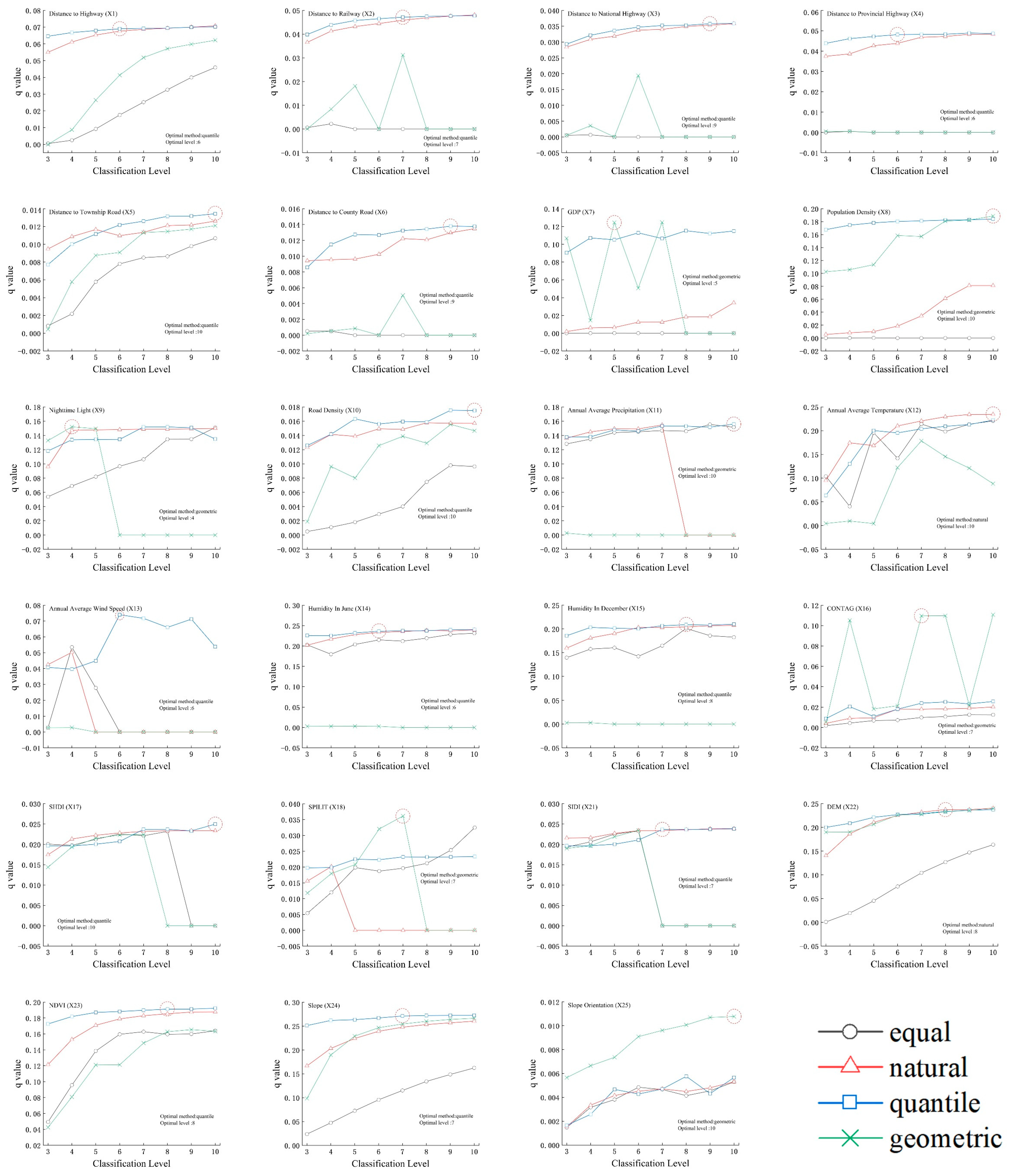
The OPGD model, developed from the geographical detector theory, is specifically designed to assess spatial heterogeneity and factor influence strength [14]. To meet the discretization requirements of the OPGD model while improving accuracy, this study incorporated four discretization schemes (equal interval, natural breaks, quantile, and geometric interval) across classification levels ranging from 3 to 10. By iteratively evaluating all parameter combinations, the discretization scheme that achieved the highest explanatory power (i.e., the maximum q-statistic) while maintaining a relatively low classification level was selected as the optimal strategy. Based on the optimized scheme, single-factor detection was used to quantify the individual explanatory power of each variable, while interaction detection was performed to assess synergistic or nonlinear enhancement effects among variables. The mathematical formulation of the model is provided below:

$$q=1-{\displaystyle \frac{\sum _{h=1}^L{N}_h{\sigma }_h^2}{N{\sigma }^2}}=1-{\displaystyle \frac{SSW}{SST}}$$

(18)

$$SSW=\sum _{h=1}^L{N}_h{\sigma }_h^2, SST=N{\sigma }^2$$

(19)

where q value measures the explanatory power of a factor, ranging from 0 to 1, with values closer to 1 indicating stronger explanatory strength. h represents a specific stratum of the explanatory variable, $N_h$ and N are the number of spatial units in stratum h and the entire study area, respectively. ${\sigma }_h^2$ and ${\sigma }^2$ denote the variances of the dependent variable Y within stratum h and across the entire region, respectively. The sum of within-stratum variances (SSW) and the sum of squares for total variation (SST) together quantify spatial heterogeneity.

3. Results

3.1. Spatiotemporal Patterns of LUCC During 2000–2020

From 2000 to 2020, China’s coastal areas exhibited a core pattern characterized by continuous farmland loss, rapid expansion of construction land, and fluctuating adjustments in woodland and grassland (Table S5 of the Supplementary Materials). Farmland experienced a cumulative reduction of 29,929 km² (single dynamic degree: −0.30%), with the loss rate during 2000–2010 (−0.42%) being 2.3 times higher than in 2010–2020 (−0.18%), reflecting intense compression of agricultural spaces by early-stage urbanization. Construction land expansion followed a “fast-then-slow” trajectory, increasing by 43,711 km² (single dynamic degree: 3.90%) over two decades, though post-2010 growth decelerated to 1.13%, temporally aligning with land-intensive policies (e.g., the National New-type Urbanization Plan, 2014–2020). Woodland shifted from net gain (2209 km², 2000–2010) to loss (−7318 km², 2010–2020), while grassland saw partial recovery post-2010 (145 km²) but overall declined by 12,903 km², highlighting regional disparities in ecological governance effectiveness.

The comprehensive LUCC dynamic degree dropped markedly from 0.28% (2000–2010) to 0.13% (2010–2020) (−53.6%), signaling a transition to stock-dominated land use, whereby land development increasingly depends on optimizing existing land resources rather than expanding into undeveloped land. This shift reflects both physical constraints on land supply and the growing emphasis on sustainable and high-efficiency land management. Water bodies expanded steadily (5704 km², single dynamic degree: 0.57%), likely due to enhanced protection against aquatic encroachment, while unused land declined sharply (−1473 km²), indicating improvements in coastal ecological rehabilitation.

Spatially, farmland loss and construction land expansion concentrated in urban agglomerations (e.g., Yangtze River Delta and Pearl River Delta) (Figure 2), correlating with population and economic density. This transition aligns with the “Three Control Lines” framework under territorial spatial planning, though woodland reversal post-2010 underscores the need for stricter ecological redline enforcement.

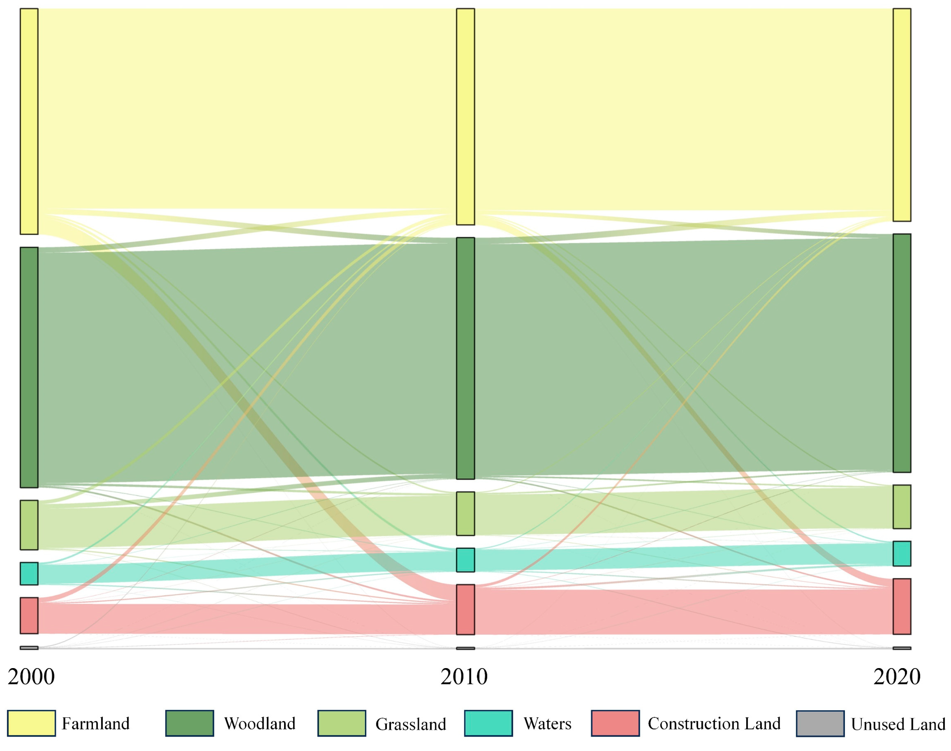
The Sankey diagram of land-use/cover transitions (Figure 3) shows that, from 2000 to 2010, land conversion was dominated by a one-way shift from farmland to construction land. This transition accounted for 78.9% of the total changes and reflects a typical urbanization-driven “farmland-to-city” model. In contrast, the period from 2010 to 2020 saw a 44% reduction in the rate of farmland loss, with farmland comprisin only 51% of newly developed construction land. Concurrently, the proportions of woodland and water bodies converted to construction land increased to 9.4% and 6.5%, respectively, reflecting a strategic shift in land supply from incremental expansion to stock optimization. Notably, bidirectional transitions between woodland and grassland became more pronounced, partially driven by ecological restoration initiatives such as reforestation of former agricultural land. However, the effectiveness of these policies remained constrained by entrenched patterns of local development.

3.2. Simulation of Land Use/Cover Under Four Scenarios in 2030

The PLUS model achieved an overall accuracy of 93.1% and a Kappa coefficient of 0.899 in simulating land use/cover in 2020, indicating strong agreement with observed land use/cover. These results demonstrate the model’s high spatial fidelity and temporal robustness, providing a reliable basis for scenario-based projections.

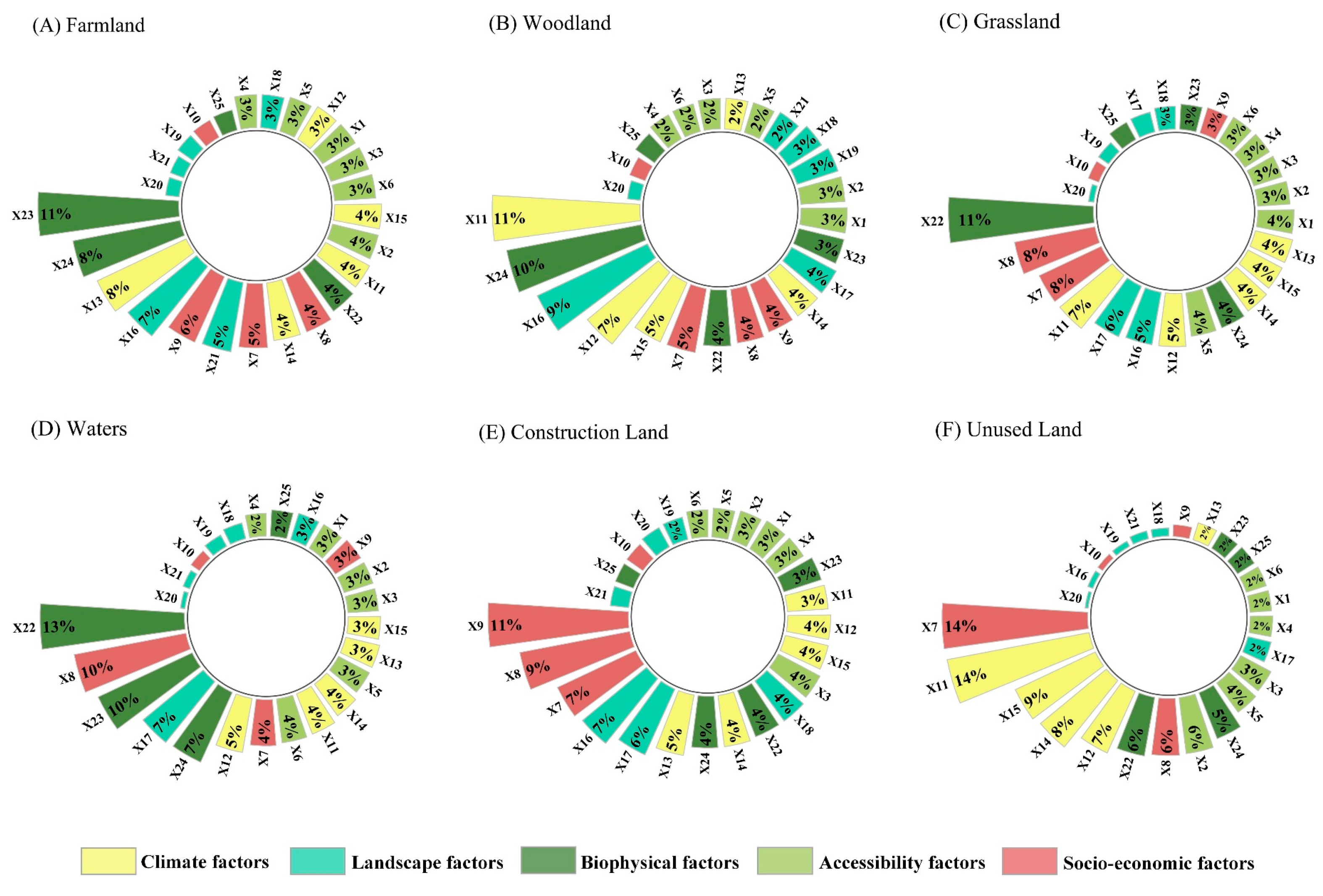
Based on the calibrated PLUS model, the LUCC patterns in China’s coastal regions from 2010 to 2020 were found to be shaped by distinct combinations of biophysical, climatic, and socioeconomic drivers, with varying contributions to the expansion of different land-use/cover types (Figure 4). Farmland expansion was primarily influenced by biophysical factors (25%), particularly the NDVI (11%) and slope (8%), highlighting the importance of vegetation and topography in determining agricultural suitability. Woodland expansion was predominantly driven by climatic factors (29%), with annual precipitation contributing 11%, underlining the critical role of water availability in forest growth. Construction land expansion was strongly associated with socioeconomic factors (27%), particularly nighttime light index (11%), population density (9%), and GDP (7%), which reflect the impact of urbanization and economic growth. Expansion of water bodies was primarily constrained by elevation (13%), especially in low-lying coastal and deltaic areas, where landforms limit water body formation. In contrast, unused land expansion was most strongly influenced by climatic variables (38%), indicating that environmental factors play a major role in restricting land development in certain regions.

The calibrated PLUS model was used to simulate land-use/cover patterns for 2030 based on the LUCC data from 2010 to 2020, incorporating land conversion costs, Markov transition probabilities, and spatial constraints. Under the NDS scenario (Figure 2 and Table S6 of the Supplementary Materials), from 2020 to 2030, construction land expanded markedly by 10,456 km² (8.4%), primarily at the expense of farmland (−7229 km²), woodland (−3979 km²), and unused land (−46 km²). Marginal increases (<0.2%) were observed in water bodies and grassland.

In the EPS scenario (Figure 2 and Table S6), urban expansion was moderated, with construction land growth reduced by 57.5% compared to the NDS scenario. This scenario also led to slight gains in farmland (1051 km²) and construction land (4701 km²), reflecting the influence of ecological constraints.

The EDS scenario (Figure 2 and Table S6) exhibited the most aggressive land conversion, with construction land surging by 30,826 km² (24.9%), threefold that of NDS, accompanied by substantial losses in farmland (−19,025 km²), woodland (−13,003 km²), and unused land (−669 km²), underscoring high-intensity development pressure. In contrast, the FPS scenario (Figure 2 and Table S6) reversed this trend, increasing farmland by 5536 km² (1.1%), a fivefold gain relative to EPS, while limiting construction land expansion to 3817 km² (0.3%). Moreover, woodland, grassland, water bodies, and unused land all declined to varying degrees, reflecting trade-offs in spatial allocation among different land-use types driven by urban expansion and agricultural development.

3.3. Spatiotemporal Patterns of Carbon Storage from 2000 to 2030

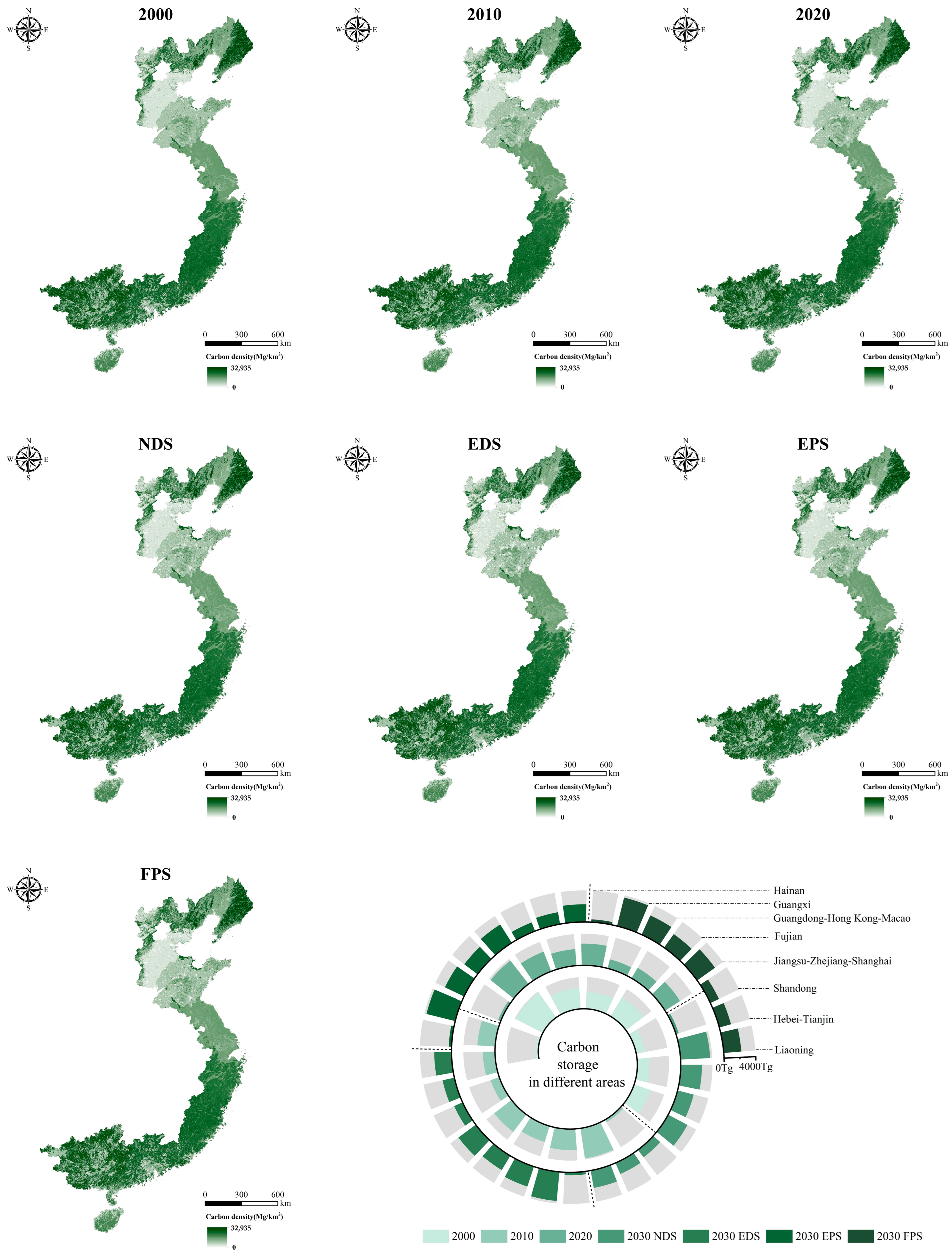
Based on the InVEST model, China’s coastal regions exhibit a distinct spatial pattern of carbon storage, characterized by a “high-north, low-central, high-south” distribution (Figure 5). High carbon storage is primarily concentrated in forest-dominated areas, including eastern Liaoning, the Zhejiang–Fujian border region, and the Guangdong–Guangxi corridor. In contrast, low values are mainly found in farmland-dominated areas, such as the Hebei, Shandong, and Jiangsu Provinces.

From 2000 to 2020, total carbon storage decreased from 16,702.17 Tg to 16,423.78 Tg (

Table 2. Different types of carbon storage in coastal areas during 2000–2030.

Year		Carbon Storage (Tg)
		Aboveground	Belowground	Dead Organic	Soil Organic	Total
2000		5235.36	1935.01	488.36	9043.44	16,702.17
2005		5229.99	1922.20	485.90	9033.90	16,671.98
2010		5244.62	1916.91	478.91	9010.37	16,650.81
2015		5219.94	1898.95	465.90	8973.79	16,558.57
2020		5176.62	1862.40	438.61	8946.16	16,423.78
2030	NDS	5136.47	1865.90	439.46	8978.90	16,420.73
	EPS	5164.86	1895.92	470.97	9002.80	16,534.55
	EDS	5107.86	1868.69	465.83	8962.97	16,405.35
	FPS	5152.86	1893.75	471.06	9016.13	16,533.80

), predominantly driven by urban expansion and the conversion of farmland to construction land. Decomposition of this loss indicates that soil organic carbon was the most affected component (−97.28 Tg, 34.94%), followed by belowground biomass (−72.61 Tg, 26.08%), aboveground biomass (−58.74 Tg, 21.10%), and dead organic matter (−49.76 Tg, 17.88%). This decomposition highlights the critical vulnerability of the soil organic carbon pool to LUCC, suggesting that soil disturbance associated with urbanization exerts a stronger impact on ecosystem carbon stocks than aboveground vegetation loss alone.

Woodland, which contributed over 59% of the total carbon storage, experienced a net reduction of 189.09 Tg during 2000–2020 (

Table 3. Proportional contribution of each land-use/cover type to total carbon storage during 2000–2030.

Land-Use/Cover Type	2000	2005	2010	2015	2020	2030
						NDS	EPS	EDS	FPS
Farmland	25.91%	25.47%	24.59%	24.41%	24.28%	22.07%	21.67%	22.00%	22.73%
Woodland	59.70%	59.75%	60.17%	60.01%	59.56%	63.12%	62.53%	63.07%	62.81%
Grassland	7.95%	7.77%	7.10%	7.10%	7.15%	7.18%	7.24%	7.16%	7.15%
Waters	2.54%	2.59%	2.81%	2.83%	3.04%	3.15%	3.28%	3.12%	3.02%
Construction Land	3.71%	4.23%	5.17%	5.48%	5.80%	4.40%	5.21%	4.57%	4.20%
Unused Land	0.20%	0.19%	0.16%	0.17%	0.17%	0.08%	0.08%	0.09%	0.09%

). Farmland, accounting for over 24% of the total carbon storage, showed a more pronounced loss of 339.61 Tg, particularly during 2005–2010. In contrast, water bodies exhibited a net gain of 75.76 Tg, while grasslands declined by 152.85 Tg. Construction land contributed an increase of 333.06 Tg, mainly due to vegetation restoration and soil accumulation in newly developed areas.

Among the four scenarios (Table 2), the EPS scenario yielded the highest carbon storage (16,534.55 Tg) by 2030, closely followed by the FPS scenario (16,533.80 Tg), NDS scenario (16,420.73 Tg), and EDS scenario (16,405.35 Tg). Relative to 2020, EPS and FPS achieved carbon gains of 110.77 Tg and 110.02 Tg, respectively, while EDS showed the largest loss (−18.43 Tg).

Scenario-specific responses highlight the differentiated effects of policy and planning. Under EPS, woodland carbon storage increased substantially by 556.76 Tg compared to 2020. The FPS scenario, emphasizing farmland protection, effectively curbs soil organic carbon loss, resulting in a 69.97 Tg increase over 2020. Although farmland carbon storage under FPS decreased by 228.55 Tg, this loss is notably smaller than that in the NDS scenario (−362.70 Tg). The EDS scenario exhibited the most severe loss in aboveground biomass (−68.86 Tg), attributable to accelerated construction land expansion. Across all scenarios, water body carbon storage increased relative to 2020, with the largest gain observed under EPS (42.71 Tg).

Notably, although EPS maintained a slightly larger farmland area (474,953 km²) than NDS (473,902 km²), its farmland carbon storage was lower (Table 3), suggesting that newly preserved farmlands in EPS are located in areas with lower carbon density. This underscores that carbon storage is jointly determined by land-use/cover type and the spatial heterogeneity of carbon density. In contrast, FPS retains significantly more farmland area (479,438 km²) and higher farmland carbon storage (3758.62 Tg) compared to NDS (3624.47 Tg), largely due to protection strategies embedded in the PLUS model. These strategies effectively prevent the conversion of high-carbon-density regions, such as long-term stable and high-quality farmland, thereby ensuring greater retention of carbon storage.

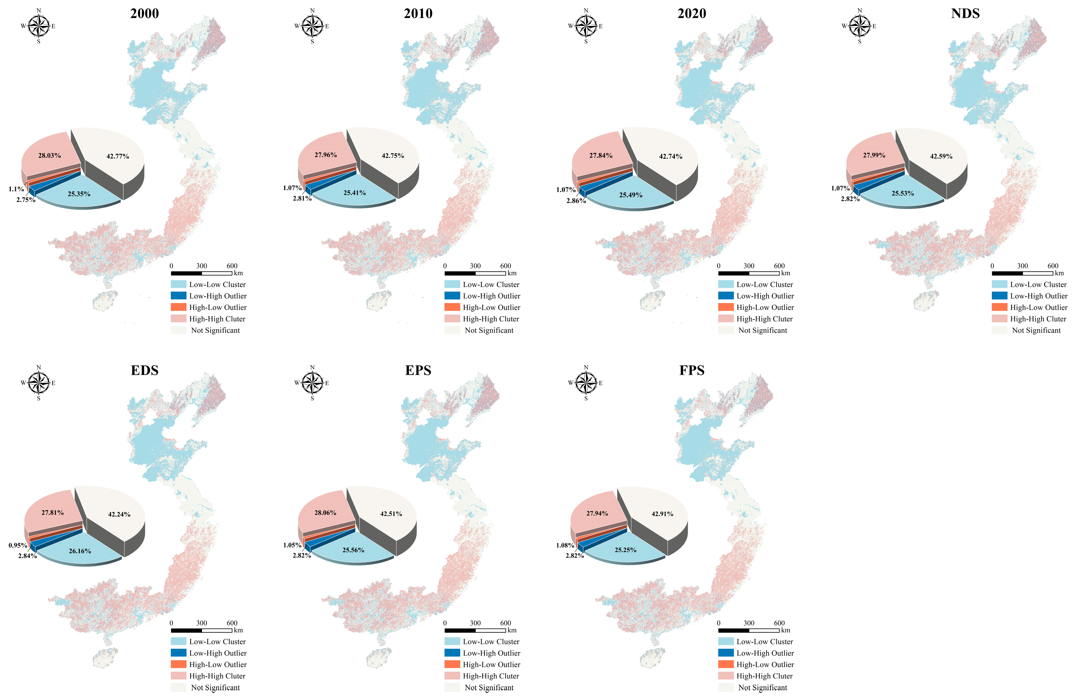
Regional carbon storage patterns exhibited pronounced spatial heterogeneity, accompanied by a continuous rise in Moran’s I, indicating an intensification of spatial dependence (Table S7 of the Supplementary Materials). The EDS scenario recorded the highest Moran’s I value, suggesting that accelerated economic development exacerbates the spatial clustering of carbon storage. LISA maps (Figure 6) further demonstrate stable high-value carbon storage clusters in forest-rich regions such as Liaoning, Zhejiang, Fujian, and non-Delta areas of Guangdong, while low-value clusters consistently emerged in heavily urbanized or agricultural zones like Hebei, Shandong, and the Pearl River Delta.

Between 2000 and 2020, the proportion of areas with high-value carbon clusters slightly declined from 28.03% to 27.84%, whereas the proportion of low-value areas increased from 25.35% to 25.53%, reflecting a sustained compression of natural carbon sinks due to intensified anthropogenic activities. Scenario-based projections reinforced this trend: under the EDS scenario, the spatial extent of high-value clusters was the smallest (27.81%), while low-value areas occupied the largest proportion (26.16%). These findings underscore the critical impact of development intensity on the spatial integrity and resilience of coastal carbon sinks.

3.4. Spatiotemporal Trend of Carbon Storage and Emissions

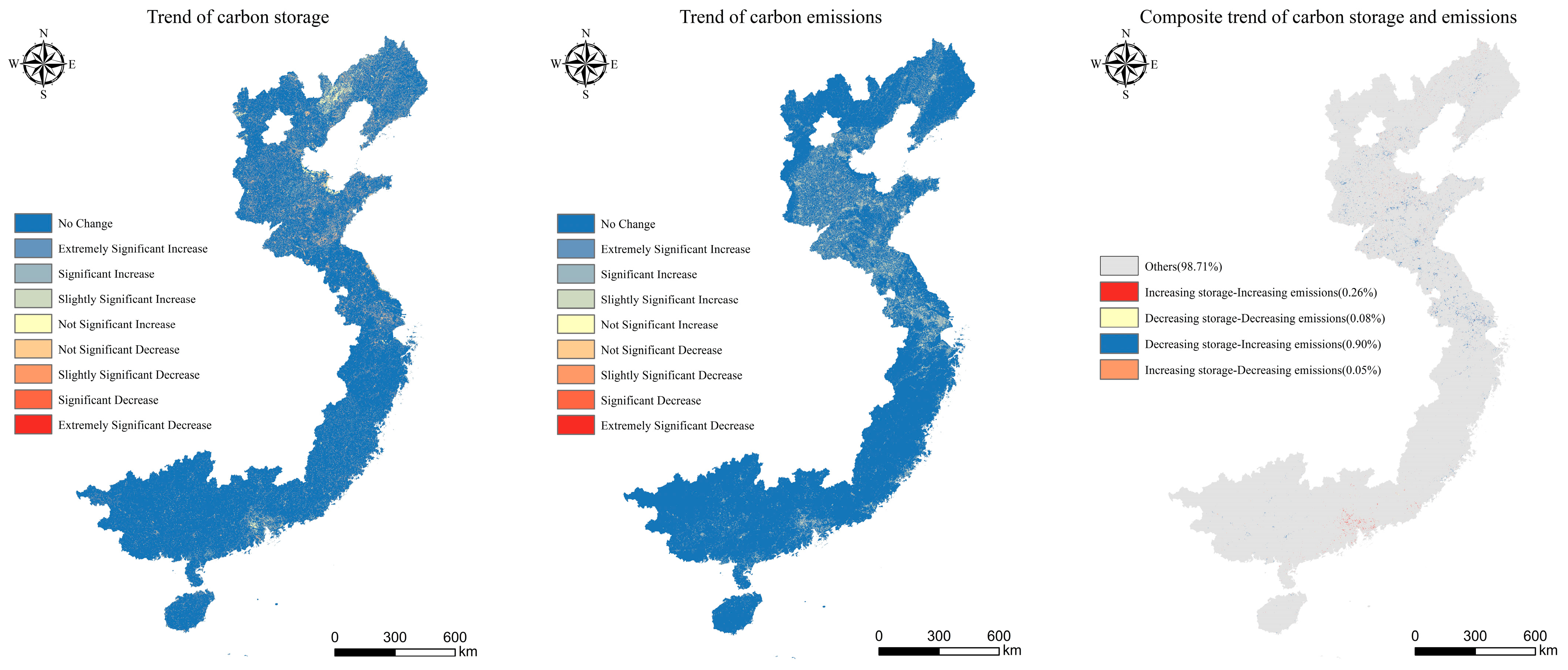
To quantify coastal dynamics in carbon storage and emissions between 2000 and 2020, we employed the Theil–Sen slope estimator in conjunction with the Mann–Kendall significance test (Figure 7). The results show that 8.09% of the carbon storage changes in the study area are statistically significant, among which 3.28% show an upward trend and 4.81% show a downward trend. The changes in carbon emissions in 7.68% of the study areas were statistically significant, among which 7.04% of the areas showed an upward trend and 0.64% of the areas showed a downward trend.

Overlay analysis of trends reveals that only 0.05% of the region simultaneously experienced increased carbon storage and reduced carbon emissions, reflecting limited areas achieving synergistic ecological gains from 2000 to 2020. In comparison, 0.90% of the region exhibited a concurrent decline in carbon storage and rise in carbon emissions, suggesting areas under intensified anthropogenic stress. Meanwhile, 0.26% of the region experienced simultaneous increases in both carbon storage and emissions, and 0.08% displayed concurrent decreases.

Provincial-level statistics (Table S8 of the Supplementary Materials) indicate that the Jiangsu–Zhejiang–Shanghai region recorded the largest area of carbon storage loss coupled with increased emissions (3774 km²), while the Guangdong–Hong Kong–Macao region showed the smallest extent (0 km²). Conversely, Shandong Province had the largest area of synergistic improvement, specifically increased carbon storage and reduced emissions (266 km²), whereas the Guangdong–Hong Kong–Macao region again recorded the smallest area (0 km²).

3.5. The Conflict and Synergy Between Carbon Storage and Emissions

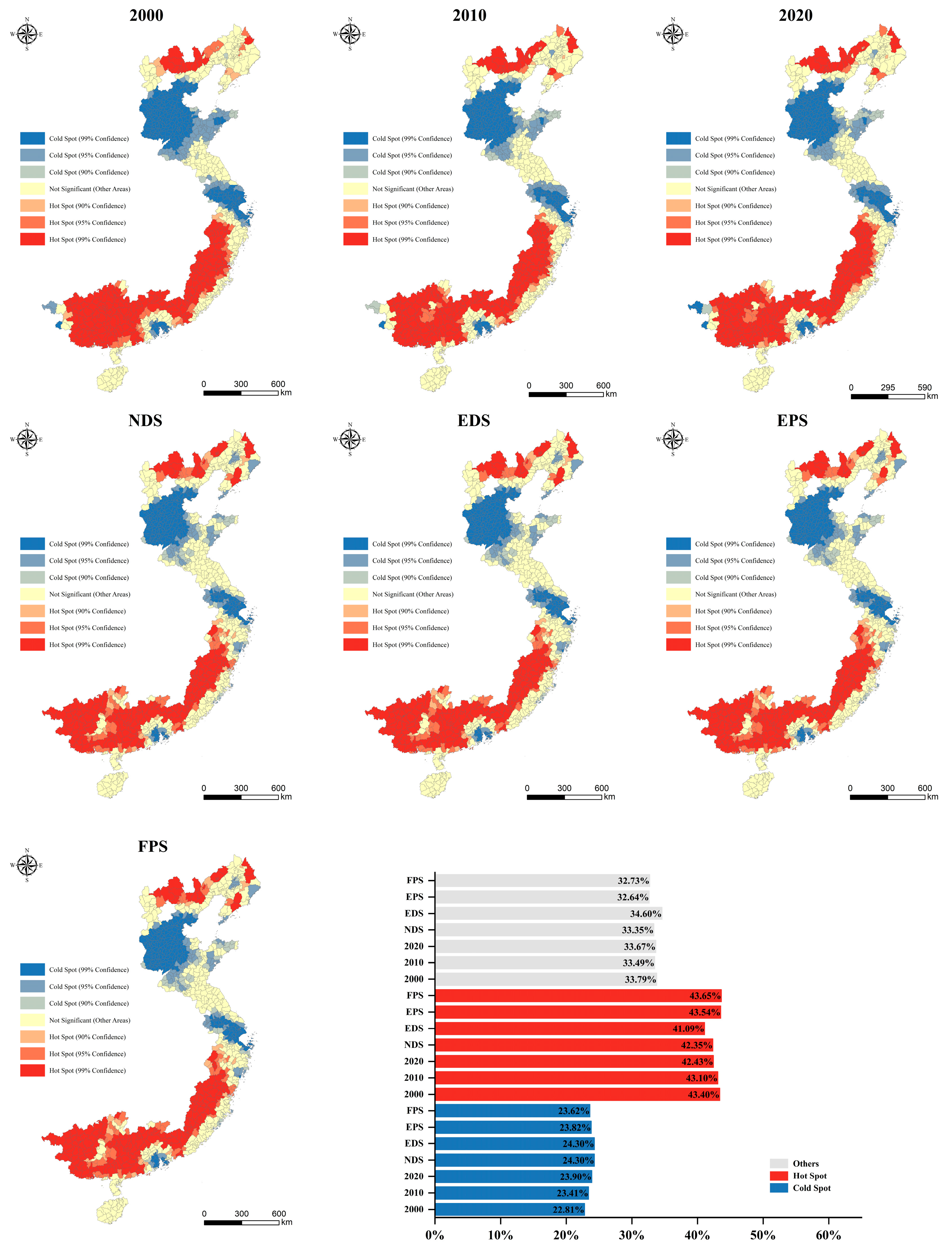
Between 2000 and 2020, the spatial extent of carbon storage hotspots exhibited a gradual decline, decreasing from 43.40% to 42.43% (Figure 8). These hotspots were consistently concentrated in ecologically stable regions, including Guangxi, inland Guangdong, Fujian, southern inland Zhejiang, and eastern Liaoning. Conversely, the proportion of carbon storage cold spots increased from 22.81% to 23.90%, with strong spatial clustering in rapidly urbanizing and industrializing zones such as the Pearl River Delta, the Yangtze River Delta, the Shandong Peninsula, the Tianjin–Hebei urban agglomeration, and western Liaoning. Among the four scenarios in 2030, the proportion of cold points in EDS and NDS is the highest (24.30%), the proportion of cold points in FPS is the lowest (23.62%), the proportion of hotspots in FPS is the highest (43.65%), and the proportion of hotspots in EDS is the lowest (41.09%).

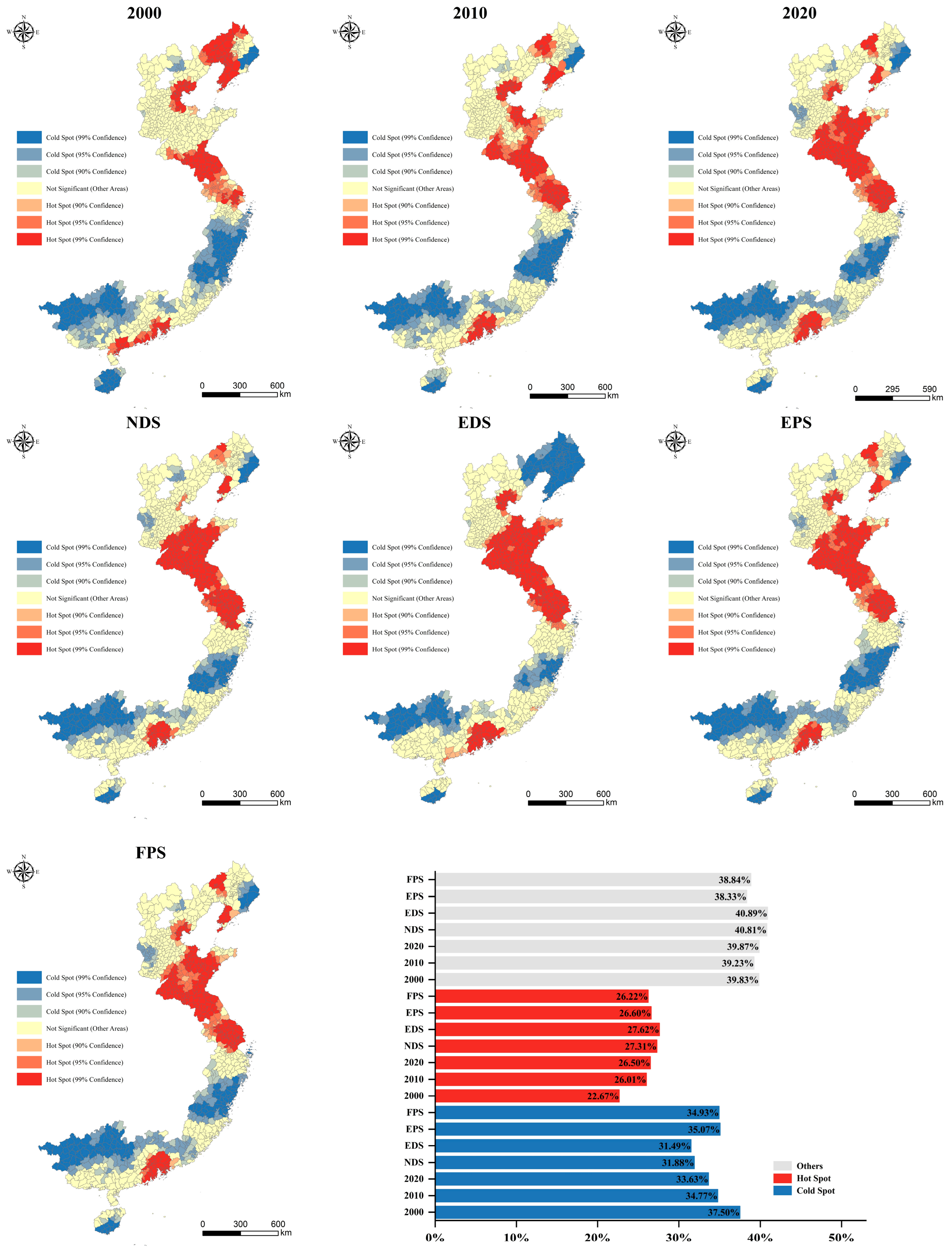
Carbon emissions displayed an opposing spatial trend. The proportion of emission hotspots increased from 22.67% in 2000 to 26.50% in 2020, predominantly located in economically developed areas including the Pearl River Delta, the Yangtze River Delta, Shandong, and Hebei (Figure 9). In contrast, the proportion of emission cold spots declined from 37.50% to 33.63%, mainly distributed in ecological conservation zones such as Guangxi, Hainan, and Fujian, as well as in northern Hebei and eastern Liaoning. This trend reflects a potential shift in environmental protection efforts or changes in regional policies affecting carbon emissions. Among the four scenarios in 2030, EPS has the highest proportion of cold spots (35.07%), EDS has the lowest proportion of cold spots (31.49%), EDS has the highest proportion of hotspots (27.62%), and FPS has the lowest proportion of hotspots (26.22%).

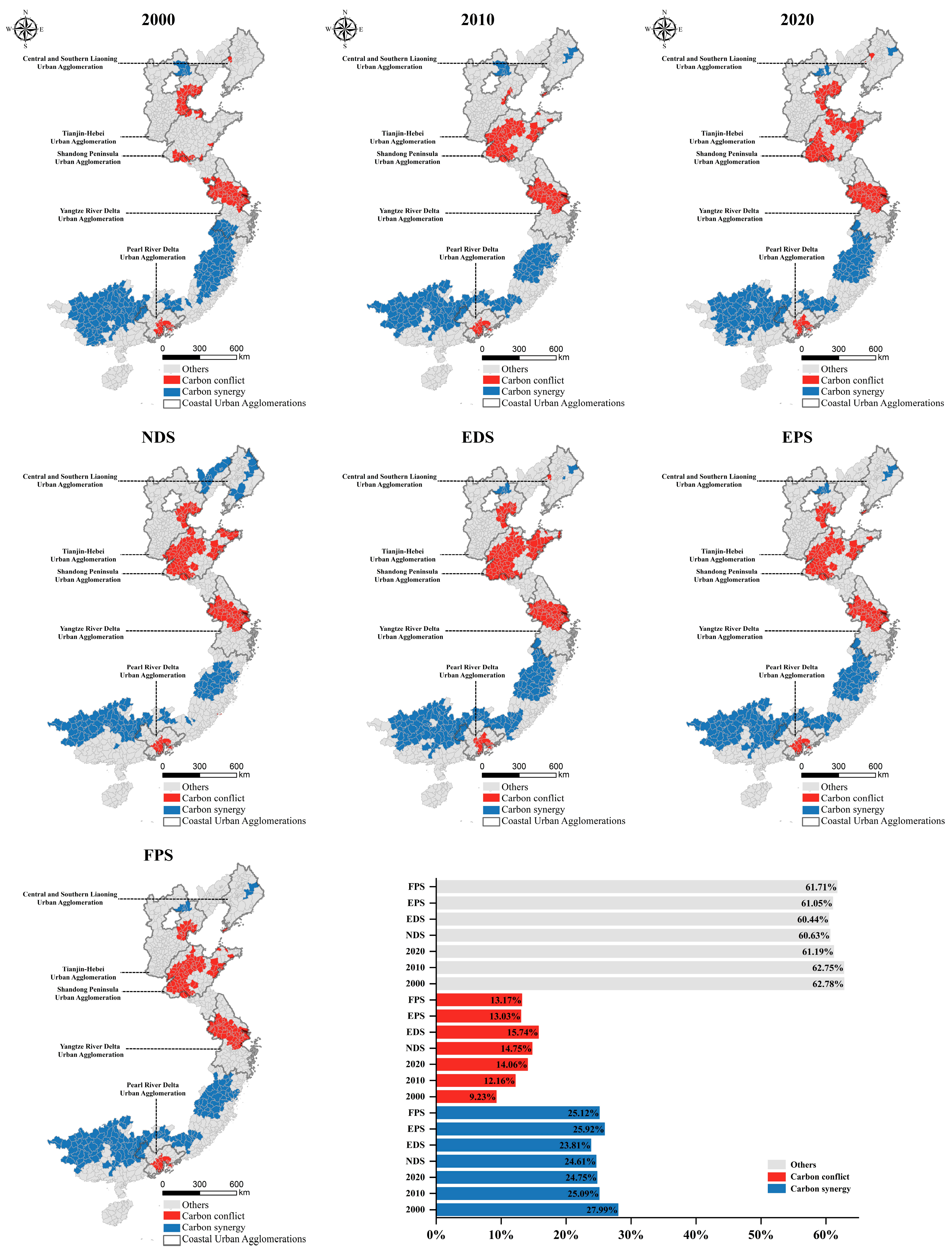
The proportion of carbon conflict areas (regions characterized by hotspots of carbon emissions and cold spots of carbon storage) steadily increased from 9.23% in 2000 to 12.06% in 2020 (Figure 10). These areas are primarily located within major urban agglomerations, with a particularly high concentration in economically active regions such as the Pearl River Delta, the Yangtze River Delta, the Shandong Peninsula, the Tianjin–Hebei region, and the central part of the Liaodong Peninsula. Conversely, the proportion of carbon synergy areas (regions with hotspots of carbon storage and cold spots of carbon emissions) decreased slightly, from 27.99% in 2000 to 24.75% in 2020. These regions are predominantly found in ecologically stable areas such as the karst landscapes of Guangxi, the hilly forested regions of Fujian, and the forest-covered zones of eastern Liaoning.

As indicated in Tables S9 and S10 of the Supplementary Materials, the Jiangsu–Zhejiang–Shanghai region exhibited the highest proportion of carbon conflict areas in 2000 (15.68%), while Shandong Province emerged as the predominant carbon conflict zone during 2010–2020 (52.40% and 50.71%, respectively). Notably, Hainan Province persistently maintained a zero-conflict status. In carbon synergy regions, Guangxi Province consistently dominated with the highest shares (78.00% in 2000, 74.47% in 2010, and 72.64% in 2020). The 2030 scenario forecast shows that under the EDS scenario; Shandong Province has the highest proportion of carbon conflicts (69.44%). Under the FPS scenario, Guangxi has the highest carbon synergy ratio (74.50%). These trends highlight the ongoing spatial dynamics of carbon emissions and storage across different regions, with significant implications for regional carbon management strategies. There is a growing challenge in balancing economic development with carbon mitigation efforts, while the stability of carbon synergy regions reflects the continued importance of ecologically favorable areas in enhancing carbon sequestration.

3.6. The Driving Mechanism of Carbon Storage–Emission Synergy in 2020

To reveal the underlying drivers of carbon storage–emission synergy in 2020, we integrated 25 potential explanatory variables (Table 1) into the OPGD model, using the spatial distribution of synergy zones as the dependent layer (Figure 10). The discretization strategy and classification methods applied to 23 continuous variables are detailed in Figure 11. We selected the classification scheme that produced the highest q value while maintaining a relatively low number of classification levels as the optimal discretization for each variable. For example, GDP (X7) exhibited the strongest explanatory power when classified using the geometric method with five levels and was therefore discretized accordingly.

Univariate factor detection results (Table S11 of the Supplementary Materials) indicate that socioeconomic, biophysical, and climatic variables exerted markedly greater influence on the spatial differentiation of carbon synergy than accessibility or landscape factors. Among all factors, the nighttime light index (X9), a proxy for human activity intensity, emerged as the dominant single driver (q = 0.254), followed closely by elevation (X22, q = 0.242) and mean annual temperature (X12, q = 0.238).

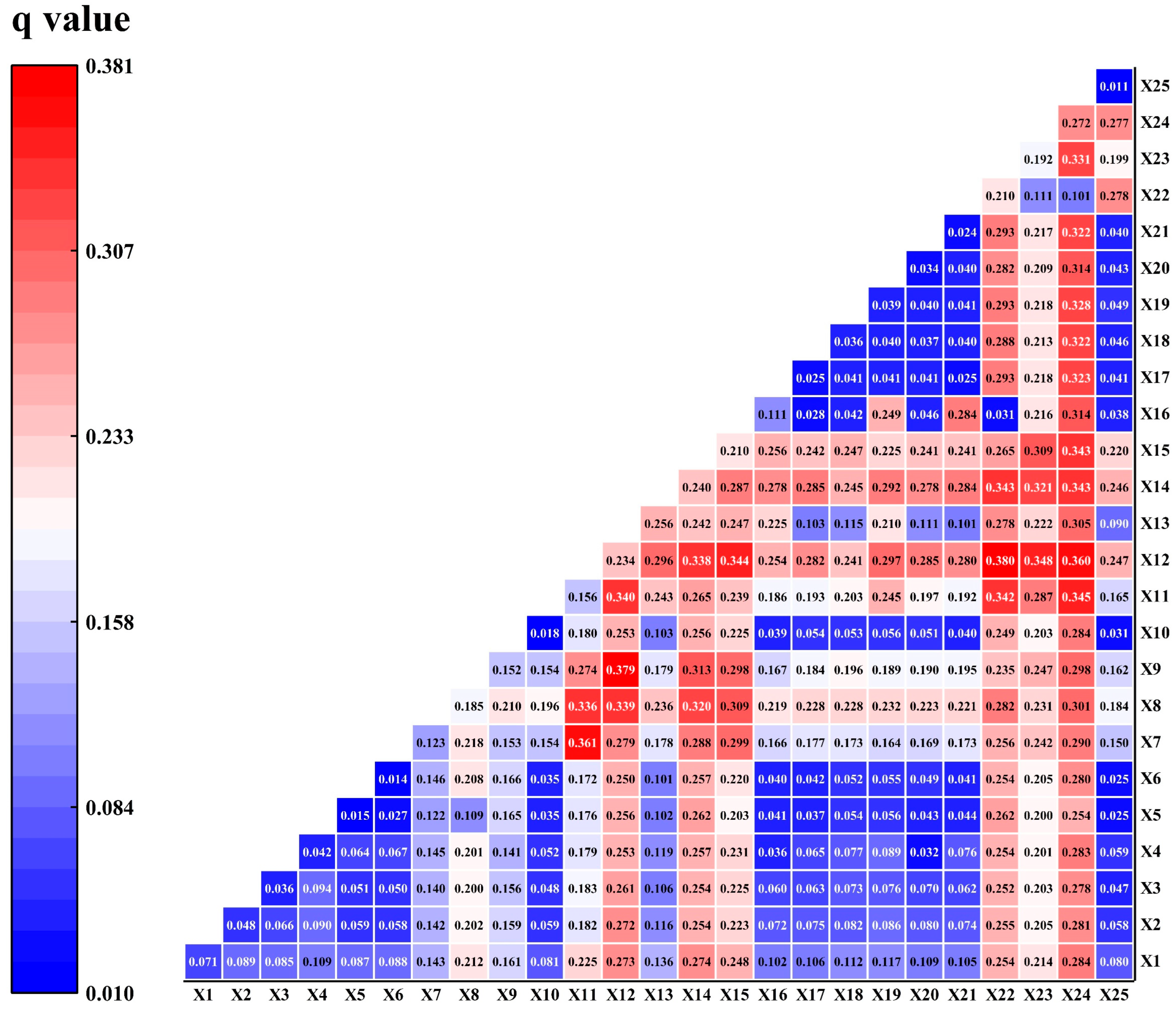
Interaction detection (Figure 12) revealed that synergistic effects were predominant across the 166 two-factor combinations tested. The most explanatory interactions included GDP and mean annual precipitation (X7 and X11, q = 0.361), nighttime light index and mean annual temperature (X9 and X12, q = 0.379), and mean annual temperature with elevation (X12 and X22, q = 0.380). These results highlight the importance of compound influences, suggesting that the spatial pattern of carbon synergy is shaped more by the joint effects of interacting variables than by any single factor alone.

4. Discussion

4.1. Advantage of the PLUS-InVEST Model in Assessing Carbon Storage

In this study, we coupled PLUS and InVEST models to assess carbon storage in China’s coastal provinces under multiple land-use scenarios projected for 2030, offering guidance for land-use planning aimed at maximizing carbon sequestration. Our findings show that the EPS scenario resulted in higher carbon storage than other scenarios (Table 2), consistent with previous studies [42,43,44]. This enhancement in carbon storage under EPS is primarily due to its emphasis on ecological land expansion and strict control of urban sprawl. By prioritizing woodland, water bodies, and grassland protection and promoting afforestation, EPS preserves high-carbon-density ecosystems and enhances sequestration capacity across coastal landscapes. Moreover, the predictive performance of the PLUS model in our study outperformed that of earlier applications. For example, Li et al. reported a Kappa coefficient of 83.74% and an overall accuracy of 90.53% when simulating 2020 land use in Hangzhou [45], which is lower than the metrics achieved in our analysis. This further supports the robustness of the coupled PLUS-InVEST framework for regional-scale carbon storage assessment under complex land-use dynamics.

Over the past three years, the PLUS-InVEST modeling framework has emerged as a robust and flexible tool for evaluating carbon storage across various spatial scales in China, from urban to national levels. For instance, Zhang et al. successfully applied this framework to simulate carbon storage changes in Chengdu [46], revealing a marked decline driven by rapid urban expansion, thereby underscoring the importance of proactive land-use planning. Similarly, Guo et al. employed the PLUS-InVEST model to analyze land use and carbon storage under different scenarios in China [47], highlighting the model’s strength in capturing spatial heterogeneity and feedback mechanisms, which are often overlooked in traditional assessment methods. Furthermore, several studies have enhanced the PLUS-InVEST framework by integrating it with external datasets and decision-support tools. For example, Guo et al. incorporated the global land-use harmonization dataset [47], which significantly improved the model’s capability of downscaling global land-use projections to regional assessments. Wang et al. further extended the model by coupling it with a system dynamics framework [48], enabling dynamic feedback between socioeconomic development and land-use transitions, thereby improving the comprehensiveness of carbon storage simulations.

However, most of these studies have focused on inland or singular metropolitan areas, with limited attention paid to coastal provinces from 2000 to 2030, which are both ecologically sensitive and economically critical. Our study addresses this gap by applying the PLUS-InVEST framework across China’s coastal provinces, regions that face intense land-use competition due to rapid urbanization, industrial development, and coastal ecosystem conservation needs.

4.2. Impacts of Human Activities, Policies, and Coastal Saltwater Intrusion on Carbon Storage Dynamics

In this study, between 2000 and 2020, the dominant driver of carbon storage loss in China’s coastal zones was the conversion of woodland and cropland into built-up areas (Table 2, Figure 3, and Table S5 in Supplementary Materials). In Jiangsu, China, reclamation of tidal flats and grasslands for cities and agriculture has further eroded carbon sequestration capacity [49], while degradation of natural wetlands in the Hebei–Tianjin region accounted for a net loss of 5.15 Tg C from 1990 to 2020 [50]. Analogous patterns emerge in tropical forests, where anthropogenic disturbances (logging and fragmentation) outstrip climatic or edaphic controls in driving carbon depletion [51]. Moreover, coastal infrastructure development frequently obliterates mangrove and saltmarsh habitats, further diminishing carbon sequestration potential. Collectively, deforestation, agricultural intensification, and urban expansion have reshaped terrestrial carbon fluxes to the coast, weakening both storage dynamics and broader biogeochemical cycling [52].

Beyond anthropogenic LUCC, climate change (e.g., rising temperatures, altered precipitation, and sea-level rise) further erodes vegetated coastal habitats and exacerbates carbon release [53,54]. Socioeconomic pressures, captured by nighttime light intensity, population density, and GDP, have predominantly driven the expansion of built-up areas (Figure 4), as seen in Jiaozhou Bay where socioeconomic development correlates with declines in both carbon stocks and annual sequestration rates [55]. Yet, concerted restoration of mangroves and macrophyte beds can reverse these losses by enhancing coastal sequestration capacity [56], and the adoption of sustainable land-use practices and urban planning can mitigate the adverse effects of human activities on coastal carbon storage [50].

Scenarios prioritizing ecological and farmland protection (EPS and FPS) consistently outperformed those emphasizing natural or economic development (NDS and EDS) in projected 2030 carbon stocks (Table 2), underscoring the power of land-use policy to steer carbon storage trajectories. In Fujian Province, EPS measures such as afforestation and strict conservation are forecast to restore regional carbon stocks to 2.02 Pg by 2030 [22]. In China, policies promoting carbon capture and storage technologies, such as the carbon emission trading system (ETS), have been shown to potentially reduce carbon emissions by 960 to 1604 Mt CO₂ annually by 2060 [57]. International experience confirms similar dynamics: Portugal’s tighter carbon regulations have driven up domestic energy sales and prices, illustrating both environmental and economic dimensions of policy [58].

On the other hand, unbalanced application of the same policy tools might produce unintended consequences. Fujian’s urban growth directives converted forest and cropland to construction areas, reversing local gains in carbon storage [22]. Additionally, in coal mining areas like Yanzhou, urbanization and village relocation driven by policy changes have led to carbon storage depletion [59]. These examples underscore the need for balanced policies that consider both development and conservation to optimize carbon storage dynamics.

The carbon storage dynamics in coastal areas are significantly influenced by their physical processes, among which the saltwater intrusion caused by sea level rise is one of the key factors. The research by De La Régola and Tali found that the salt migration driven by saltwater intrusion directly changed the carbon storage pattern, and the soil carbon reservoirs distributed along the riverbanks changed the most significantly. This study further pointed out that the soil carbon storage is more sensitive to humidity than to electrical conductivity and pH value [60]. The farmland facing saltwater intrusion is at the forefront of climate response, and its scientific management is of crucial significance for maintaining the existing soil carbon reservoir and enhancing the future carbon sequestration potential. The research by Charles et al. revealed another impact of saltwater intrusion: it erodes the organic carbon reservoirs in coastal wetlands rich in organic matter, causing a decrease in the surface elevation of the wetlands and subsequently promoting the degradation of the wetlands into open waters. This process weakens the ecosystem’s resilience in restoring its elevation, thereby reducing its resistance to sea level rise (SLR). This indicates that the organic carbon reservoirs in coastal wetlands play a decisive role in maintaining the survival ability of freshwater and brackish water wetlands [61].

4.3. The Synergy and Conflict Between Carbon Storage and Carbon Emissions

The synergy and conflict between carbon storage and carbon emissions in China’s coastal provinces from 2000 to 2020 reflect a complex interplay of urbanization, industrialization, and ecological management. During this period, carbon conflict regions steadily expanded, while the carbon synergy regions contracted, shrinking from 6.9 times to just 5.8 times the area of conflict zones (Figure 10), highlighting the challenges of balancing economic growth with environmental sustainability. The significant increase in carbon emissions (Figure 9), particularly in urbanized and economically vibrant areas, contrasts with the decline in carbon storage in China’s coastal provinces (Table 2), underscoring the need for integrated strategies to manage carbon dynamics effectively. This situation is further complicated by the spatial distribution of carbon sources and sinks [62], which varies significantly across different regions (Figure 5, Figure 6, Figure 7, Figure 8, Figure 9 and Figure 10).

Carbon conflict regions are predominantly found in highly urbanized areas with dense transport networks (Figure 10), where rapid coastal industrialization has driven up emissions [63] and the conversion of farmland and forests to built-up land has depleted carbon stocks [52]. Conversely, carbon synergy regions, often located in sparsely populated and heavily forested zones (Figure 10), maintain stronger carbon sinks, which are crucial for long-term sustainability. While the focus on reducing carbon emissions and enhancing carbon storage is crucial, it is important to consider the broader socioeconomic context. The pursuit of energy security and equity can sometimes conflict with environmental sustainability goals, as seen in the varying levels of conflict across China’s coastal provinces (Figure 10). Additionally, the role of forests in carbon management is complex; while increasing forest areas can help, effective management and investment in forest activities are essential for maximizing their carbon sequestration potential [64]. These insights highlight the need for a balanced approach that considers both ecological and socioeconomic factors in carbon management strategies.

In response to the national “dual carbon” strategy, carbon conflict zones urgently need to promote the low-carbon transformation of the industrial structure and the clean transformation of the energy system. As the core carrier of carbon sequestration, the carbon synergy zone should strengthen the rigid constraints of the ecological protection red line and strictly curb the occupation of construction land.

4.4. The Driving Mechanism of Carbon Synergy Using the OPGD Model

The OPGD model is a powerful tool for understanding the spatial distribution of carbon synergy regions, identifying key drivers such as socioeconomic factors (population density and nighttime light index), climatic factors (mean annual temperature and precipitation), and terrain factors (elevation) (Figure 12). By adaptively tuning data discretization thresholds, class-break counts, and analysis scales, OPGD captures fine-scale heterogeneity in both natural and anthropogenic variables [14]. Previous applications underscore OPGD’s versatility in eco-environmental research. In a karst watershed, for example, OPGD pinpointed NDVI, population density, human activity intensity, slope, and lithology as predominant controls on carbon-stock fluctuations [65]. Likewise, when applied to net primary productivity (NPP) dynamics, the model isolated elevation, temperature, NDVI, topographic relief, and LUCC as principal determinants of spatial NPP variation [66].

Higher population densities often correlate with increased carbon emissions due to intensified human activities and energy consumption [67]. The nighttime light index serves as a proxy for human activity and economic development, significantly impacting carbon emissions. Studies have shown that regions with higher nighttime light index tend to have higher carbon emissions, due to increased industrial and commercial activities [68]. The interaction between nighttime light index and other factors, such as elevation and slope, further enhances its impact on carbon storage heterogeneity [69]. Moreover, temperature and precipitation fluctuations impact the carbon sequestration potential of terrestrial ecosystems. Elevated temperatures and precipitation can reduce soil carbon and affect plant physiological processes, altering carbon source–sink relationships [70]. Conversely, in some regions, milder climates may reduce energy demands. On the other side, the relationship between elevation and carbon dynamics is complex and often nonlinear, as it involves interactions between climatic conditions, vegetation types, soil properties, and microbial activities. In subtropical forests in Pakistan, carbon pools are negatively associated with elevation, with higher carbon stocks at lower elevations. This is attributed to changes in species composition and biomass distribution along the elevation gradient [71].

The interaction between socioeconomic and natural factors is crucial in understanding carbon dynamics. For instance, the combination of high population density and elevated temperatures can exacerbate carbon emissions, while regions with lower population densities and cooler climates may act as carbon sinks [72]. Hence, insights from the OPGD model can inform policy and planning efforts aimed at reducing carbon emissions and enhancing carbon storage, such as optimizing land-use patterns and promoting energy-efficient urban designs.

4.5. Limitations and Future Perspectives

Despite the strengths of our integrated PLUS-InVEST and OPGD framework for assessing coastal China’s carbon storage and carbon emissions trajectories (2000–2030) and elucidating the drivers of carbon-emission synergy, several limitations warrant consideration.

This study simulated the EDS by adjusting land-use transition probabilities. These adjustments caused construction land expansion under EDS to triple compared to the NDS. Since future carbon storage and emissions depend on fixed coefficients multiplied by land-use area, transition probabilities critically shape future spatial patterns and carbon outcomes. The PLUS model’s probabilities were calibrated using literature data, lacking rigorous empirical validation and assessment of the impact of minor probability changes. This limits the clarity of the scenarios’ robustness. Future research should therefore quantitatively analyze the sensitivity of land-use distribution and carbon results to transition probability changes to enhance simulation rigor and policy relevance.

While the OPGD effectively identifies spatial drivers and interactions underlying carbon synergy zones, it may oversimplify the inherent nonlinear feedback and threshold effects in complex carbon cycles. Furthermore, as model calibration was confined to China’s coastal provinces, its transferability to other biogeographic contexts requires validation and recalibration. Therefore, future research will couple OPGD with nonlinear models. This approach will help identify key nonlinear drivers by combining feature importance analysis with the q-statistic. It will also detect critical thresholds using change-point analysis or generalized additive models (GAMs), improving our understanding of the mechanisms behind areas of carbon synergy and conflict.

While our carbon density inputs (Table S1 of the Supplementary Materials) primarily drew upon measured data near the eight study sub-regions and averaged multi-source data within the same areas, the reliance on provincial-level averages inadequately captured intra-regional heterogeneity. This static carbon density assumption risks overestimating carbon sequestration benefits from land-use conversion and underestimating sequestration in naturally regenerating ecosystems. Due to the lack of measured carbon storage data in the coastal areas of China, the accuracy of carbon storage cannot be reliably evaluated. This data gap will reduce the reliability and application value of future carbon scenario simulations. The ecosystems distributed along the coast of China, such as mangroves, salt marshes, and seagrass beds, have high heterogeneity, and their carbon storage shows significant spatial differentiation. The absence of cross-checking with actual data often leads to model reliance on parameters from similar areas, ignoring local characteristics and causing systematic deviations in the simulation results. Although Zhu et al. assessed accuracy for some sub-regions [73], their study used sparse and temporally inconsistent field data, fundamentally constrained by the scarcity of large-scale and continuous time-series measurements. Future research should establish a more comprehensive field measurement system.

Land-use change is the main cause of the instability and uncertainty of carbon storage in terrestrial ecosystems [74]. Therefore, assessing the uncertainty and instability of carbon sources/sinks in this context and analyzing the mechanisms is crucial for understanding ecosystem services, and this is also the deficiency of this study and the direction that future research needs to focus on. For example, Zhou et al. evaluated the uncertainty of carbon storage simulations [75], indicating that the instability of carbon storage increased from 2000 to 2020, and it is expected that the uncertainty will significantly decrease from 2020 to 2035. Among them, the uncertainty is the highest in the urban expansion scenario and the lowest in the ecological protection scenario.

5. Conclusions

This study presents a comprehensive assessment of the spatiotemporal dynamics of carbon storage and emissions in China’s coastal regions by integrating the PLUS-InVEST and OPGD modeling frameworks, and it identified the key driving mechanisms of carbon synergy. The major findings are summarized as follows:

(1)

Coastal China experienced significant LUCC from 2000 to 2020, characterized by rapid urbanization-driven farmland loss and construction land expansion. This transition led to a net decline in carbon storage, primarily due to soil organic carbon depletion and biomass loss.

(2)

Land-use scenarios that prioritize ecological and farmland protection had greater potential for enhancing carbon storage by 2030, highlighting the critical role of policy-driven land management in shaping future carbon dynamics.

(3)

Carbon synergy zones are concentrated in forests and sparsely populated areas, while conflict zones are concentrated in urban agglomerations. Under EDS and NDS, the conflict areas have expanded significantly; under EPS and FPS, the synergy zones have significantly expanded.

(4)

Carbon synergy was predominantly influenced by the interaction of socioeconomic (population density and nighttime light index) and natural factors (mean annual temperature, mean annual precipitation, and elevation), emphasizing the need for integrated land–climate policy frameworks.

(5)

Future research should fully consider the dynamic changes in carbon density and carbon emission coefficients over time and in response to the growth status of vegetation. At the same time, attention should be paid to the issue of uncertainty propagation in land-use and carbon prediction models. Moreover, the PLUS-Invest-OPGD framework should be extended and applied to global coastal areas to reveal the multi-scale spatial patterns of carbon synergy and conflict. These efforts will significantly enhance the scientific basis and policy guidance value of climate mitigation strategies based on land in the context of global climate change.

References

1. Hu, C.; Wang, Z.; Wang, Y.; Sun, D.; Zhang, J. Combining MSPA-MCR Model to Evaluate the Ecological Network in Wuhan, China. Land 2022, 11, 213. [Google Scholar] [CrossRef]
2. Zhu, E.; Qi, Q.; Chen, L.; Wu, X. The Spatial-Temporal Patterns and Multiple Driving Mechanisms of Carbon Emissions in the Process of Urbanization: A Case Study in Zhejiang, China. J. Clean. Prod. 2022, 358, 131954. [Google Scholar] [CrossRef]
3. Zhong, R.; Pu, L.; Xie, J.; Yao, J.; Qie, L.; He, G.; Wang, X.; Zhang, R.; Zhai, J.; Gong, Z.; et al. Carbon Storage in Typical Ecosystems of Coastal Wetlands in Jiangsu, China: Spatiotemporal Patterns and Mechanisms. CATENA 2025, 254, 108882. [Google Scholar] [CrossRef]
4. Wang, H.; Guo, J. Research on the Impact Mechanism of Multiple Environmental Regulations on Carbon Emissions under the Perspective of Carbon Peaking Pressure: A Case Study of China’s Coastal Regions. Ocean. Coast. Manag. 2024, 249, 106985. [Google Scholar] [CrossRef]
5. Xu, S.; Zhang, S.; Pan, Y.; Liu, X.; Welsch, E.; Ma, X.; Guo, C.; Dai, H. Health Equity and Synergistic Abatement Strategies of Carbon Dioxide and Air Pollutant Emissions Reduction in China’s Eastern Coastal Area. Environ. Res. Lett. 2024, 19, 104023. [Google Scholar] [CrossRef]
6. Tang, X.; Zhao, X.; Bai, Y.; Tang, Z.; Wang, W.; Zhao, Y.; Wan, H.; Xie, Z.; Shi, X.; Wu, B.; et al. Carbon Pools in China’s Terrestrial Ecosystems: New Estimates Based on an Intensive Field Survey. Proc. Natl. Acad. Sci. USA 2018, 115, 4021–4026. [Google Scholar] [CrossRef]
7. Yang, K.; Zhou, P.; Wu, J.; Yao, Q.; Yang, Z.; Wang, X.; Wen, Y. Carbon Stock Inversion Study of a Carbon Peaking Pilot Urban Combining Machine Learning and Landsat Images. Ecol. Indic. 2024, 159, 111657. [Google Scholar] [CrossRef]
8. Li, P.; Chen, J.; Li, Y.; Wu, W. Using the InVEST-PLUS Model to Predict and Analyze the Pattern of Ecosystem Carbon Storage in Liaoning Province, China. Remote Sens. 2023, 15, 4050. [Google Scholar] [CrossRef]
9. Li, C.; Xu, H.; Du, P.; Tang, F. Predicting Land Cover Changes and Carbon Stock Fluctuations in Fuzhou, China: A Deep Learning and InVEST Approach. Ecol. Indic. 2024, 167, 112658. [Google Scholar] [CrossRef]
10. Li, C.; Wu, Y.; Gao, B.; Zheng, K.; Wu, Y.; Li, C. Multi-Scenario Simulation of Ecosystem Service Value for Optimization of Land Use in the Sichuan-Yunnan Ecological Barrier, China. Ecol. Indic. 2021, 132, 108328. [Google Scholar] [CrossRef]
11. Wei, Q.; Abudureheman, M.; Halike, A.; Yao, K.; Yao, L.; Tang, H.; Tuheti, B. Temporal and Spatial Variation Analysis of Habitat Quality on the PLUS-InVEST Model for Ebinur Lake Basin, China. Ecol. Indic. 2022, 145, 109632. [Google Scholar] [CrossRef]
12. Xiong, L.; Wang, M.; Mao, J.; Huang, B. A Review of Building Carbon Emission Accounting Methods under Low-Carbon Building Background. Buildings 2024, 14, 777. [Google Scholar] [CrossRef]
13. Wang, J.; Li, X.; Christakos, G.; Liao, Y.; Zhang, T.; Gu, X.; Zheng, X. Geographical Detectors-Based Health Risk Assessment and Its Application in the Neural Tube Defects Study of the Heshun Region, China. Int. J. Geogr. Inf. Sci. 2010, 24, 107–127. [Google Scholar] [CrossRef]
14. Song, Y.; Wang, J.; Ge, Y.; Xu, C. An Optimal Parameters-Based Geographical Detector Model Enhances Geographic Characteristics of Explanatory Variables for Spatial Heterogeneity Analysis: Cases with Different Types of Spatial Data. GISci. Remote Sens. 2020, 57, 593–610. [Google Scholar] [CrossRef]
15. Zheng, Z.; Wu, Z.; Chen, Y.; Yang, Z.; Marinello, F. Exploration of Eco-Environment and Urbanization Changes in Coastal Zones: A Case Study in China over the Past 20 Years. Ecol. Indic. 2020, 119, 106847. [Google Scholar] [CrossRef]
16. GB/T 21010-2017; Current Land Use Classification. General Administration of Quality Supervision, Inspection and Quarantine of the People’s Republic of China, Standardization Administration of the People’s Republic of China: Beijing, China, 2017.
17. Xu, X.; Li, D.; Liu, H.; Zhao, G.; Cui, B.; Yi, Y.; Yang, W.; Du, J. Comparative Validation and Misclassification Diagnosis of 30-Meter Land Cover Datasets in China. Remote Sens. 2024, 16, 4330. [Google Scholar] [CrossRef]
18. Jiang, H.; Cui, Z.; Fan, T.; Yin, H. Impacts of Land Use Change on Carbon Storage in the Guangxi Beibu Gulf Economic Zone Based on the PLUS-InVEST Model. Sci. Rep. 2025, 15, 6468. [Google Scholar] [CrossRef]
19. Lei, J.; Zhang, L.; Chen, Z.; Wu, T.; Chen, X.; Li, Y. The Impact of Land Use Change on Carbon Storage and Multi-Scenario Prediction in Hainan Island Using InVEST and CA-Markov Models. Front. For. Glob. Change 2024, 7, 1349057. [Google Scholar] [CrossRef]
20. Wu, W.; Huang, Z.; Sun, Z.; Zhang, J.; Wang, S.; Fang, M.; Yang, H.; Lu, H.; Guo, G.; Liu, W. Simulation and Attribution Analysis of Terrestrial Ecosystem Carbon Storage of Hainan Island from 2015 to 2050. Sci. Total Environ. 2024, 917, 170348. [Google Scholar] [CrossRef]
21. Wang, W.; Hu, Y.; Mao, X.; Zhang, Y.; Tang, L.; Cai, J. Terrestrial Carbon Storage Estimation in Guangdong Province (2000–2021). Data 2025, 10, 41. [Google Scholar] [CrossRef]
22. Nie, Q.; Man, W.; Li, Z.; Wu, X. From Policy to Practice: Assessing Carbon Storage in Fujian Province Using Patch-Generating Land Use Simulation and Integrated Valuation of Ecosystem Services and Tradeoffs Models. Land 2025, 14, 179. [Google Scholar] [CrossRef]
23. Zhang, X.; Wang, J.; Yue, C.; Ma, S.; Wang, L.-J. Exploring the Spatiotemporal Changes in Carbon Storage under Different Development Scenarios in Jiangsu Province, China. PeerJ 2022, 10, e13411. [Google Scholar] [CrossRef] [PubMed]
24. Wang, Y.; Jiang, X.; Gao, S.; Jiang, Q.; Du, H.; Han, N. Multi-Scenario Carbon Storage Analysis Based on PLUS Model and InVEST Model: A Case Study of Zhejiang Province, China. Earth Sci. Inform. 2025, 18, 192. [Google Scholar] [CrossRef]
25. Zheng, H.; Zheng, H. Assessment and Prediction of Carbon Storage Based on Land Use/Land Cover Dynamics in the Coastal Area of Shandong Province. Ecol. Indic. 2023, 153, 110474. [Google Scholar] [CrossRef]
26. He, Y.; Xia, C.; Shao, Z.; Zhao, J. The Spatiotemporal Evolution and Prediction of Carbon Storage: A Case Study of Urban Agglomeration in China’s Beijing-Tianjin-Hebei Region. Land 2022, 11, 858. [Google Scholar] [CrossRef]
27. Rong, T.; Zhang, P.; Zhu, H.; Jiang, L.; Li, Y.; Liu, Z. Spatial Correlation Evolution and Prediction Scenario of Land Use Carbon Emissions in China. Ecol. Inform. 2022, 71, 101802. [Google Scholar] [CrossRef]
28. IPCC. 2019 Refinement to the 2006 IPCC Guidelines for National Greenhouse gas Inventory. Agric. For. Other Land Use 2019, 4, 824. [Google Scholar]
29. Hu, C.; Wang, Z.; Huang, G.; Ding, Y. Construction, Evaluation, and Optimization of a Regional Ecological Security Pattern Based on MSPA–Circuit Theory Approach. Int. J. Environ. Res. Public. Health 2022, 19, 16184. [Google Scholar] [CrossRef]
30. Liu, X.; Andersson, C. Assessing the Impact of Temporal Dynamics on Land-Use Change Modeling. Comput. Environ. Urban Syst. 2004, 28, 107–124. [Google Scholar] [CrossRef]
31. Guo, R.; Wu, T.; Wu, X.; Luigi, S.; Wang, Y. Simulation of Urban Land Expansion Under Ecological Constraints in Harbin-Changchun Urban Agglomeration, China. Chin. Geogr. Sci. 2022, 32, 438–455. [Google Scholar] [CrossRef]
32. Liang, X.; Guan, Q.; Clarke, K.C.; Liu, S.; Wang, B.; Yao, Y. Understanding the Drivers of Sustainable Land Expansion Using a Patch-Generating Land Use Simulation (PLUS) Model: A Case Study in Wuhan, China. Comput. Environ. Urban Syst. 2021, 85, 101569. [Google Scholar] [CrossRef]
33. Tang, W.; Hu, J.; Zhang, H.; Wu, P.; He, H. Kappa Coefficient: A Popular Measure of Rater Agreement. Shanghai Arch. Psychiatry 2015, 27, 62–67. [Google Scholar] [CrossRef] [PubMed]
34. Nie, W.; Xu, B.; Yang, F.; Shi, Y.; Liu, B.; Wu, R.; Lin, W.; Pei, H.; Bao, Z. Simulating Future Land Use by Coupling Ecological Security Patterns and Multiple Scenarios. Sci. Total Environ. 2023, 859, 160262. [Google Scholar] [CrossRef] [PubMed]
35. Zafar, Z.; Zubair, M.; Zha, Y.; Mehmood, M.S.; Rehman, A.; Fahd, S.; Nadeem, A.A. Predictive Modeling of Regional Carbon Storage Dynamics in Response to Land Use/Land Cover Changes: An InVEST-Based Analysis. Ecol. Inform. 2024, 82, 102701. [Google Scholar] [CrossRef]
36. Alam, S.A.; Starr, M.; Clark, B.J.F. Tree Biomass and Soil Organic Carbon Densities across the Sudanese Woodland Savannah: A Regional Carbon Sequestration Study. J. Arid. Environ. 2013, 89, 67–76. [Google Scholar] [CrossRef]
37. He, Y.; Ma, J.; Zhang, C.; Yang, H. Spatio-Temporal Evolution and Prediction of Carbon Storage in Guilin Based on FLUS and InVEST Models. Remote Sens. 2023, 15, 1445. [Google Scholar] [CrossRef]
38. Anselin, L. Local Indicators of Spatial Association—LISA. Geogr. Anal. 1995, 27, 93–115. [Google Scholar] [CrossRef]
39. Tian, S.; Wang, S.; Bai, X.; Luo, G.; Li, Q.; Yang, Y.; Hu, Z.; Li, C.; Deng, Y. Global Patterns and Changes of Carbon Emissions from Land Use during 1992–2015. Environ. Sci. Ecotechnology 2021, 7, 100108. [Google Scholar] [CrossRef]
40. Hubau, W.; Lewis, S.L.; Phillips, O.L.; Affum-Baffoe, K.; Beeckman, H.; Cuní-Sanchez, A.; Daniels, A.K.; Ewango, C.E.N.; Fauset, S.; Mukinzi, J.M.; et al. Asynchronous Carbon Sink Saturation in African and Amazonian Tropical Forests. Nature 2020, 579, 80–87. [Google Scholar] [CrossRef]
41. Yang, S.; Yang, X.; Gao, X.; Zhang, J. Spatial and Temporal Distribution Characteristics of Carbon Emissions and Their Drivers in Shrinking Cities in China: Empirical Evidence Based on the NPP/VIIRS Nighttime Lighting Index. J. Environ. Manage. 2022, 322, 116082. [Google Scholar] [CrossRef]
42. Zhao, S.; Zhou, D.; Wang, D.; Chen, J.; Gao, Y.; Zhang, J.; Jiang, J. Ecosystem Carbon Storage Assessment and Multi-Scenario Prediction in the Weihe River Basin Based on PLUS-InVEST Model. Chin. J. Appl. Ecol. 2024, 35, 2044–2054. [Google Scholar] [CrossRef]
43. Fu, S.; Zhen, Z.; Zhou, H.; Wang, B.; Qiao, Q. Spatio-Temporal Evolution and Prediction of Carbon Storage at the Source of the Fen River and Sanggan River Based on a PLUS-InVEST Model. Front. Environ. Sci. 2024, 12, 1449576. [Google Scholar] [CrossRef]
44. Li, J.; Hu, J.; Kang, J.; Shu, W. Spatio-Temporal Variation and Prediction of Land Use and Carbon Storage Based on PLUS-InVEST Model in Shanxi Province, China. Landsc. Ecol. Eng. 2025, 21, 107–119. [Google Scholar] [CrossRef]
45. Li, Y.; Yao, S.; Jiang, H.; Wang, H.; Ran, Q.; Gao, X.; Ding, X.; Ge, D. Spatial-Temporal Evolution and Prediction of Carbon Storage: An Integrated Framework Based on the MOP–PLUS–InVEST Model and an Applied Case Study in Hangzhou, East China. Land 2022, 11, 2213. [Google Scholar] [CrossRef]
46. Zhang, Y.; Liao, X.; Sun, D. A Coupled InVEST-PLUS Model for the Spatiotemporal Evolution of Ecosystem Carbon Storage and Multi-Scenario Prediction Analysis. Land 2024, 13, 509. [Google Scholar] [CrossRef]
47. Guo, W.; Teng, Y.; Li, J.; Yan, Y.; Zhao, C.; Li, Y.; Li, X. A New Assessment Framework to Forecast Land Use and Carbon Storage under Different SSP-RCP Scenarios in China. Sci. Total Environ. 2024, 912, 169088. [Google Scholar] [CrossRef]
48. Wang, Q.; Zhang, W.; Xia, J.; Ou, D.; Tian, Z.; Gao, X. Multi-Scenario Simulation of Land-Use/Land-Cover Changes and Carbon Storage Prediction Coupled with the SD-PLUS-InVEST Model: A Case Study of the Tuojiang River Basin, China. Land 2024, 13, 1518. [Google Scholar] [CrossRef]
49. Yuan, H.; Zhang, J.; Wang, Z.; Qian, Z.; Wang, X.; Xu, W.; Zhang, H. Multi-Temporal Change of LULC and Its Impact on Carbon Storage in Jiangsu Coastal, China. Land 2023, 12, 1943. [Google Scholar] [CrossRef]
50. Zhao, L.; Gao, H.; Liu, J.; Wang, F.; Fu, T. Modeling, Assessment, and Prediction of Carbon Storage in Hebei–Tianjin Coastal Wetlands. Remote Sens. 2024, 16, 4428. [Google Scholar] [CrossRef]
51. Pyles, M.V.; Magnago, L.F.S.; Maia, V.A.; Pinho, B.X.; Pitta, G.; de Gasper, A.L.; Vibrans, A.C.; dos Santos, R.M.; van den Berg, E.; Lima, R.A.F. Human Impacts as the Main Driver of Tropical Forest Carbon. Sci. Adv. 2022, 8, eabl7968. [Google Scholar] [CrossRef]
52. Wei, B.; Mollenhauer, G.; Kusch, S.; Hefter, J.; Grotheer, H.; Schefuß, E.; Geibert, W.; Ransby, D.; Jia, G. Anthropogenic Perturbations Change the Quality and Quantity of Terrestrial Carbon Flux to the Coastal Ocean. J. Geophys. Res. Biogeosciences 2023, 128, e2023JG007482. [Google Scholar] [CrossRef]
53. Guild, R.; Wang, X.; Quijón, P.A. Climate Change Impacts on Coastal Ecosystems. Environ. Res. Clim. 2025, 3, 042006. [Google Scholar] [CrossRef]
54. Lopes, C.L.; Sousa, M.; Picado, A.; Dias, J.M. Climate Change Challenges on Coastal Environments: Physical Processes in Upwelling and Estuarine Systems. In Zooplankton Challenges in a Changing World; CRC Press: Boca Raton, FL, USA, 2025; ISBN 978-1-032-66227-5. [Google Scholar]
55. Zhang, L.; Guan, Q.; Li, H.; Chen, J.; Meng, T.; Zhou, X. Assessment of Coastal Carbon Storage and Analysis of Its Driving Factors: A Case Study of Jiaozhou Bay, China. Land 2024, 13, 1208. [Google Scholar] [CrossRef]
56. Watanabe, K.; Tokoro, T.; Moki, H.; Kuwae, T. Contribution of Marine Macrophytes to pCO2 and DOC Variations in Human-Impacted Coastal Waters. Biogeochemistry 2024, 167, 831–848. [Google Scholar] [CrossRef]
57. Fan, J.-L.; Zhou, W.; Ding, Z.; Zhang, X. The Substantial Impacts of Carbon Capture and Storage Technology Policies on Climate Change Mitigation Pathways in China. Glob. Environ. Change 2024, 86, 102847. [Google Scholar] [CrossRef]
58. Morão, H. The Impact of Carbon Policy News on the National Energy Industry. Energy Econ. 2024, 134, 107596. [Google Scholar] [CrossRef]
59. Fu, Y.; He, Y.; Chen, W.; Xiao, W.; Ren, H.; Shi, Y.; Hu, Z. Dynamics of Carbon Storage Driven by Land Use/Land Cover Transformation in Coal Mining Areas with a High Groundwater Table: A Case Study of Yanzhou Coal Mine, China. Environ. Res. 2024, 247, 118392. [Google Scholar] [CrossRef]
60. de la Reguera, E.; Tully, K.L. Farming Carbon: The Link between Saltwater Intrusion and Carbon Storage in Coastal Agricultural Fields. Agric. Ecosyst. Environ. 2021, 314, 107416. [Google Scholar] [CrossRef]
61. Charles, S.P.; Kominoski, J.S.; Troxler, T.G.; Gaiser, E.E.; Servais, S.; Wilson, B.J.; Davis, S.E.; Sklar, F.H.; Coronado-Molina, C.; Madden, C.J.; et al. Experimental Saltwater Intrusion Drives Rapid Soil Elevation and Carbon Loss in Freshwater and Brackish Everglades Marshes. Estuaries Coasts 2019, 42, 1868–1881. [Google Scholar] [CrossRef]
62. Lin, J.; Guo, Y.; Li, J.; Shao, M.; Yao, P. Spatial and Temporal Characteristics of Carbon Emission and Sequestration of Terrestrial Ecosystems and Their Driving Factors in Mainland China—A Case Study of 352 Prefectural Administrative Districts. Front. Ecol. Evol. 2023, 11, 1169427. [Google Scholar] [CrossRef]
63. Cui, L.; Tang, W.; Zheng, S.; Singh, R.P. Ecological Protection Alone Is Not Enough to Conserve Ecosystem Carbon Storage: Evidence from Guangdong, China. Land 2023, 12, 111. [Google Scholar] [CrossRef]
64. Aziz, G.; Mighri, Z. Carbon Dioxide Emissions and Forestry in China: A Spatial Panel Data Approach. Sustainability 2022, 14, 12862. [Google Scholar] [CrossRef]
65. Li, Y.; Geng, H. Spatiotemporal Trends in Ecosystem Carbon Stock Evolution and Quantitative Attribution in a Karst Watershed in Southwest China. Ecol. Indic. 2023, 153, 110429. [Google Scholar] [CrossRef]
66. Wang, G.; Peng, W.; Zhang, L.; Zhang, J. Quantifying the Impacts of Natural and Human Factors on Changes in NPP Using an Optimal Parameters-Based Geographical Detector. Ecol. Indic. 2023, 155, 111018. [Google Scholar] [CrossRef]
67. Guo, Q.; Lai, X.; Jia, Y.; Wei, F. Spatiotemporal Pattern and Driving Factors of Carbon Emissions in Guangxi Based on Geographic Detectors. Sustainability 2023, 15, 15477. [Google Scholar] [CrossRef]
68. Wang, L.; Zhang, N.; Deng, H.; Wang, P.; Yang, F.; Qu, J.J.; Zhou, X. Monitoring Urban Carbon Emissions from Energy Consumption over China with DMSP/OLS Nighttime Light Observations. Theor. Appl. Climatol. 2022, 149, 983–992. [Google Scholar] [CrossRef]
69. Lu, L.; Xue, Q.; Zhang, X.; Qin, C.; Jia, L. Spatiotemporal Variation and Quantitative Attribution of Carbon Storage Based on Multiple Satellite Data and a Coupled Model for Jinan City, China. Remote Sens. 2023, 15, 4472. [Google Scholar] [CrossRef]
70. Dotaniya, M.L.; Rajendiran, S.; Meena, B.P.; Meena, A.L.; Dotaniya, C.K.; Meena, B.L.; Jat, R.L.; Saha, J.K. Elevated Carbon Dioxide (CO2) and Temperature Vis-a-Vis Carbon Sequestration Potential of Global Terrestrial Ecosystem. In Conservation Agriculture: An Approach to Combat Climate Change in Indian Himalaya; Bisht, J.K., Meena, V.S., Mishra, P.K., Pattanayak, A., Eds.; Springer: Singapore, 2016; pp. 225–256. ISBN 978-981-10-2558-7. [Google Scholar]
71. Khan, I.; Hayat, U.; Lushuang, G.; Khan, F.; Xinyi, H.; Shufan, W. Association of Carbon Pool with Vegetation Composition along the Elevation Gradients in Subtropical Forests in Pakistan. Forests 2024, 15, 1395. [Google Scholar] [CrossRef]
72. Chen, G.; Peng, Q.; Fan, Q.; Lin, W.; Su, K. Spatial-Temporal Variation and Driving Forces of Carbon Storage at the County Scale in China Based on a Gray Multi-Objective Optimization-Patch-Level Land Use Simulation-Integrated Valuation of Ecosystem Services and Tradeoffs-Optimal Parameter-Based Geographical Detector Model: Taking the Daiyun Mountain’s Rim as an Example. Land 2025, 14, 14. [Google Scholar] [CrossRef]
73. Zhu, L.; Song, R.; Sun, S.; Li, Y.; Hu, K. Land Use/Land Cover Change and Its Impact on Ecosystem Carbon Storage in Coastal Areas of China from 1980 to 2050. Ecol. Indic. 2022, 142, 109178. [Google Scholar] [CrossRef]
74. Chang, X.; Xing, Y.; Wang, J.; Yang, H.; Gong, W. Effects of Land Use and Cover Change (LUCC) on Terrestrial Carbon Stocks in China between 2000 and 2018. Resour. Conserv. Recycl. 2022, 182, 106333. [Google Scholar] [CrossRef]
75. Zhou, H.; Tang, M.; Huang, J.; Zhang, J.; Huang, J.; Zhao, H.; Yu, Y. Instability and Uncertainty of Carbon Storage in Karst Regions under Land Use Change: A Case Study in Guiyang, China. Front. Environ. Sci. 2025, 13, 1551050. [Google Scholar] [CrossRef]
Figure 1. Location of the study area. The elevation is derived from the 1 km resolution digital elevation model (DEM) from Geospatial Data Cloud, https://www.gscloud.cn (accessed on 1 August 2024).
Remotesensing 17 02859 g001
Figure 2. Spatial distribution of land-use/cover types in coastal China during 2000–2030.
Remotesensing 17 02859 g002
Figure 3. Sankey diagram of land-use/cover transitions from 2000 to 2020.
Remotesensing 17 02859 g003
Figure 4. Contribution of the driving factors to the expansion of each land use/cover from 2010 to 2020.
Remotesensing 17 02859 g004
Figure 5. Spatial distribution of carbon storage in coastal areas during 2000–2030.
Remotesensing 17 02859 g005
Figure 6. Spatial distribution of LISA for carbon storage in coastal areas during 2000–2030.
Remotesensing 17 02859 g006
Figure 7. Spatial distribution of heterogeneity in carbon storage and emission trends.
Remotesensing 17 02859 g007
Figure 8. The spatial distribution of hotspots in carbon storage from 2000 to 2030.
Remotesensing 17 02859 g008
Figure 9. The spatial distribution of hotspots in carbon emissions from 2000 to 2030.
Remotesensing 17 02859 g009
Figure 10. The spatial distribution of carbon conflict and carbon synergy regions during 2000–2030.
Remotesensing 17 02859 g010
Figure 11. Optimized discretization parameters for the 23 continuous variables used in the OPGD model. Note that X19 and X20 are already categorical variables and were therefore excluded from further discretization (The points marked by the red dotted circles are the points corresponding to the optimal classification method and optimal classification level.).
Remotesensing 17 02859 g011
Figure 12. The q values of interaction detection for all pairwise combinations among the 25 driving factors.
Remotesensing 17 02859 g012