Article

“Ground–Aerial–Satellite” Atmospheric Correction Method Based on UAV Hyperspectral Data for Coastal Waters

by
Xinyuan Su
1,
Jianyong Cui
1,*,
Jinying Zhang
2,
Jie Guo
3,
Mingming Xu
1 and
Wenwen Gao
1
1
College of Oceanography and Space Informatics, China University of Petroleum (East China), Qingdao 266580, China
2
Shandong Provincial Institute of Land Surveying and Mapping, Jinan 250101, China
3
Yantai Institute of Coastal Zone Research, Chinese Academy of Sciences, Yantai 264003, China
*
Author to whom correspondence should be addressed.
Remote Sens. 2025, 17(16), 2768; https://doi.org/10.3390/rs17162768 (registering DOI)
Submission received: 8 July 2025 / Revised: 6 August 2025 / Accepted: 7 August 2025 / Published: 9 August 2025

Abstract

In ocean color remote sensing, most of the radiative energy received by sensors comes from the atmosphere, requiring highly accurate atmospheric correction. Although atmospheric correction models based on ground measurements—especially the Ground-Aerial-Satellite Atmospheric Correction (GASAC) method that integrates multi-scale synchronous data—are theoretically optimal, their application in nearshore areas is limited by the lack of synchronous samples, pixel mismatches, and nonlinear atmospheric effects. This study focuses on Tangdao Bay in Qingdao, Shandong Province, China, and proposes an innovative GASAC method for nearshore waters using synchronized surface spectrometer data and UAV hyperspectral imagery collected during Sentinel-2 satellite overpasses. The method first resolves pixel mismatch issues in UAV data through Pixel-by-Pixel Matching (MPP) and applies the Empirical Line Model (ELM) for high-accuracy ground-aerial atmospheric correction. Then, based on spectrally unified UAV and satellite data, a large amount of high-quality spatial atmospheric reference data is obtained. Finally, a Transformer model optimized by an Exponential-Trigonometric Optimization (ETO) algorithm is used to fit nonlinear atmospheric effects and perform aerial-to-satellite correction, forming a stepwise GASAC framework. The results show that GASAC achieves high accuracy and good generalization in local areas, with predicted remote sensing reflectance reaching R 2   =   0 .962 and R M S E = 12.54 × 10⁻⁴ sr−1, improving by 5.2% and 23.5%, respectively, over the latest deep learning baseline. In addition, the corrected data achieved R2 = 0.866 in a Chl-a retrieval model based on in situ measurements, demonstrating strong application potential. This study offers a precise and generalizable atmospheric correction method for satellite imagery in nearshore water quality monitoring, with important value for coastal aquatic ecological sensing.

1. Introduction

Atmospheric correction (AC) plays a critical role in quantitative remote sensing, particularly in water color remote sensing. Due to significant atmospheric absorption and scattering effects, as well as the complex radiative transfer processes at the water–air interface, up to 90% of the optical signal received by satellite sensors is unrelated to water constituents [1]. This makes atmospheric interference the primary limiting factor for the accuracy and reliability of water quality inversion models. Consequently, water color remote sensing places exceptionally high demands on the precision of satellite-based atmospheric correction [2,3]. Ground measurements conducted using analytical spectral devices (ASD) under rigorous observation protocols and calibration procedures can effectively eliminate atmospheric interference and yield high-precision, continuous water spectra [4]. Therefore, atmospheric correction models based on in situ measurements—referred to as ground-measured atmospheric correction (GAC)—are theoretically the most effective. However, the limited number of in situ water surface spectral samples and the poor spatiotemporal consistency with satellite remote sensing data pose significant challenges for the widespread application of GAC methods [5].
Depending on the source of the remote sensing data requiring correction, GAC can be categorized into three modes: ground–satellite atmospheric correction (GSAC), ground–aerial atmospheric correction (GAAC), and the integrated ground–aerial–satellite atmospheric correction (GASAC). The main factors limiting the accuracy of all three approaches can be summarized into three core challenges. First, it is difficult to accurately match high-resolution remote sensing data with in situ measurements. During spectral data acquisition, environmental disturbances such as water movement and the drift of the sampling vessel may cause the corresponding image pixel to poorly represent the true sampling location [6]. This issue is especially pronounced in ultra-high-resolution UAV (Unmanned Aerial Vehicle) imagery. Additionally, satellite-based water color remote sensing faces challenges such as poor temporal synchronization with field data and the presence of mixed pixels due to limited spatial resolution. Furthermore, water vapor and aerosols in coastal areas exhibit nonlinear spatial distributions both horizontally and vertically [7]. To date, aided by hyperspectral UAVs and machine learning algorithms, some progress has been made in applying GASAC for atmospheric correction in terrestrial remote sensing [8,9]. However, the three major challenges outlined above remain insufficiently addressed, thus limiting the application potential of GASAC in aquatic environments.
From a methodological perspective, traditional atmospheric correction methods in water color remote sensing can be classified into three main types: physically based methods derived from radiative transfer theory (e.g., MODTRAN, 6S, FLAASH) [10,11], the “black pixel” method based on the zero-reflectance assumption in specific bands [12], and empirical correction methods based on in situ data [13]. Unfortunately, these conventional AC methods often struggle to achieve satisfactory performance in nearshore waters. Physically based methods simulate light propagation through the atmosphere and water bodies, but they are highly sensitive to atmospheric parameters. In coastal regions, aerosol properties exhibit significant spatiotemporal variability, and the associated instruments required to acquire accurate real-time parameters are expensive and difficult to deploy. The lack of reliable atmospheric input data often results in poor correction accuracy. The “black pixel” approach assumes that water bodies exhibit near-zero reflectance in near-infrared (NIR), shortwave infrared (SWIR), or ultraviolet (UV) bands. The effectiveness of this method depends heavily on the suitability of the water body to this assumption. In coastal environments, hydrosol backscattering in poor water conditions often leads to random noise or complete failure of the method [14]. Empirical methods require simultaneous observation of ground-truth reflectance during data acquisition and establish relationships with corresponding satellite pixels to estimate atmospheric effects through regression-based modeling of the radiative transfer equation [15]. Research has shown that within small regions, near-surface atmospheric effects can be simplified as linear, and a relatively small number of correction samples is sufficient for model construction [16]. However, empirical models developed from UAV and in situ measurements over localized areas are often difficult to generalize or transfer to larger spatial domains.
With the powerful nonlinear fitting capabilities of machine learning and deep learning techniques, many limitations of traditional atmospheric correction (AC) methods in complex aerosol environments of nearshore waters have been effectively mitigated. Based on core technologies, deep learning-based ground-measured atmospheric correction (GAC) methods can be categorized into radiative transfer model-based approaches, physics-aware methods, and data-driven methods [17]. Radiative transfer model-based methods first employ machine learning to estimate difficult-to-obtain atmospheric parameters such as aerosol optical depth (AOD) and water vapor column, and then solve for surface reflectance using lookup tables (LUTs) [18]. The other two approaches directly learn the nonlinear relationship between top-of-atmosphere (TOA) inputs and in situ measurements to generate surface reflectance; the difference lies in that physics-aware methods require some auxiliary meteorological parameters [19], whereas data-driven methods do not [20]. Although these models achieve better AC accuracy than traditional methods, their generalization capabilities remain limited [19], falling short of meeting the high-precision water quality inversion demands in nearshore local waters characterized by small-sample scenarios.
In recent years, the Transformer architecture based on multi-head self-attention mechanisms has significantly enhanced the fitting capacity of deep learning networks and has been increasingly applied in quantitative remote sensing, showing promise for AC tasks in nearshore waters [21,22]. However, the scarcity of GAC samples in these environments often fails to satisfy the training requirements of deep learning architectures, thereby limiting the potential of Transformers. Therefore, it is necessary to develop a lightweight network architecture and employ efficient and rational optimization strategies to guide Transformer parameter settings, specifically optimizing key parameters such as the number of attention heads, embedding dimension of the encoder, number of neurons in the hidden layers, and initial weights and biases, thereby fully leveraging its excellent nonlinear fitting ability to improve both the accuracy and regional generalization of GAC.
Addressing the challenges of applying GASAC in nearshore waters, this study leverages synchronously collected hyperspectral UAV data as a bridge to establish a stepwise GASAC approach based on a Transformer model calibrated with ASD data for Sentinel-2 imagery. First, a pixel-wise matching method, the Matching Pixel Pool (MPP) [23], is used to match UAV pixels with ASD measurements, enabling empirical ground–aerial atmospheric correction (GAAC). Subsequently, a lightweight Transformer model is designed and optimized via the ETO strategy to achieve high-precision fitting of nonlinear atmospheric effects in nearshore waters, thus realizing aerial–satellite atmospheric correction (ASAC) and constructing a stepwise GASAC model.

2. Materials and Methods

2.1. Study Area

The study area is located in Tangdao Bay, Huangdao District, Qingdao, Shandong Province, China, with its center point at about 35°56′N, 120°11′E and an area of about 17.2 km2. It is adjacent to the Yellow Sea in the south and Jiaozhou Bay in the east and situated in the most socially and economically active area of Huangdao District. It is northeast-southwest oriented, with an estuary about 2 km wide, a narrow central ditch about 200 m wide and 6–7 km long, with water depths ranging from 2 m to 7 m, and a muddy bottom. The semi-closed structure of the bay hinders the dispersion of pollutants, and the water color is significantly affected by natural factors and human activities.
The UAV imaging area is located near the northern shore of the bay at the estuary. In the early years, this area served as a sewage outlet, carrying large amounts of industrial and domestic pollutants. In recent years, under the effective control of the local government, the water quality at the estuary has improved significantly. Studying the changes in water quality in this area is of great significance for evaluating the impact of local human activities on the coastal water environment (Displayed in Figure 1).

2.2. Data Acquisition and Preprocessing

This section mainly describes the sources of experimental data and details about data acquisition and preprocessing. The experimental data mainly includes the measured hyperspectral data of the water body, measured Chl-a concentration data, UAV hyperspectral images, and Sentinel-2 multispectral images.

2.2.1. Measured Hyperspectral Data of the Water Body

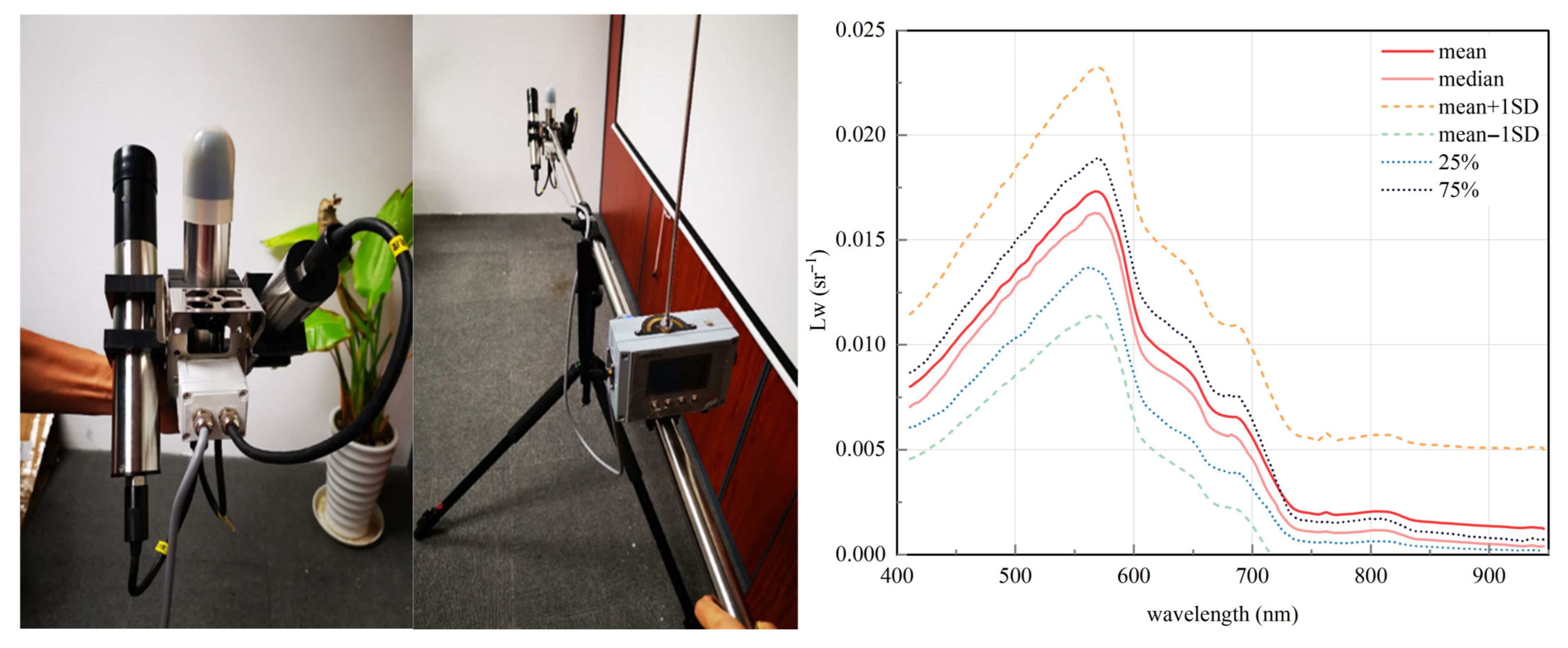
From 2022 to 2024, the experimental team onboard the research vessel collected 127 pieces of valid hyperspectral data at the location shown in Figure 1 through seven rounds of sampling using a TriOS Above-Water Radiance Mobile Measuring System (AWRMMS). As shown in Figure 2, the measuring system consists of three probes for measuring the downward solar irradiance at the water surface, solar irradiance, and sky radiance, respectively. Fifteen measurements were made at each sampling point, and the average value of all measurements was taken. The effects of sky radiance and solar irradiance were removed using the data processing software of the server, and the water-leaving radiance and remote-sensing reflectance were determined. The seven experiments (rounds of sampling) were all conducted in clear-sky, cloudless, and low-wind conditions. Considering the transit of Sentinel-2 at about 10:50 a.m., the in situ hyperspectral data was collected during the period between 10:00 a.m. and 13:00 p.m. while ensuring that the difference in observation window is controlled within two hours. Due to sufficient sunlight during this period, the measured data is accurate and reliable. The performance parameters of the measuring device and some observation geometry requirements are summarized in Table 1, and the statistical spectral curves of measured data are shown in Figure 2. The hyperspectral data of the water body measured by this device will be referred to as ASD data hereinafter.

2.2.2. Measured Chl-a Concentration Data

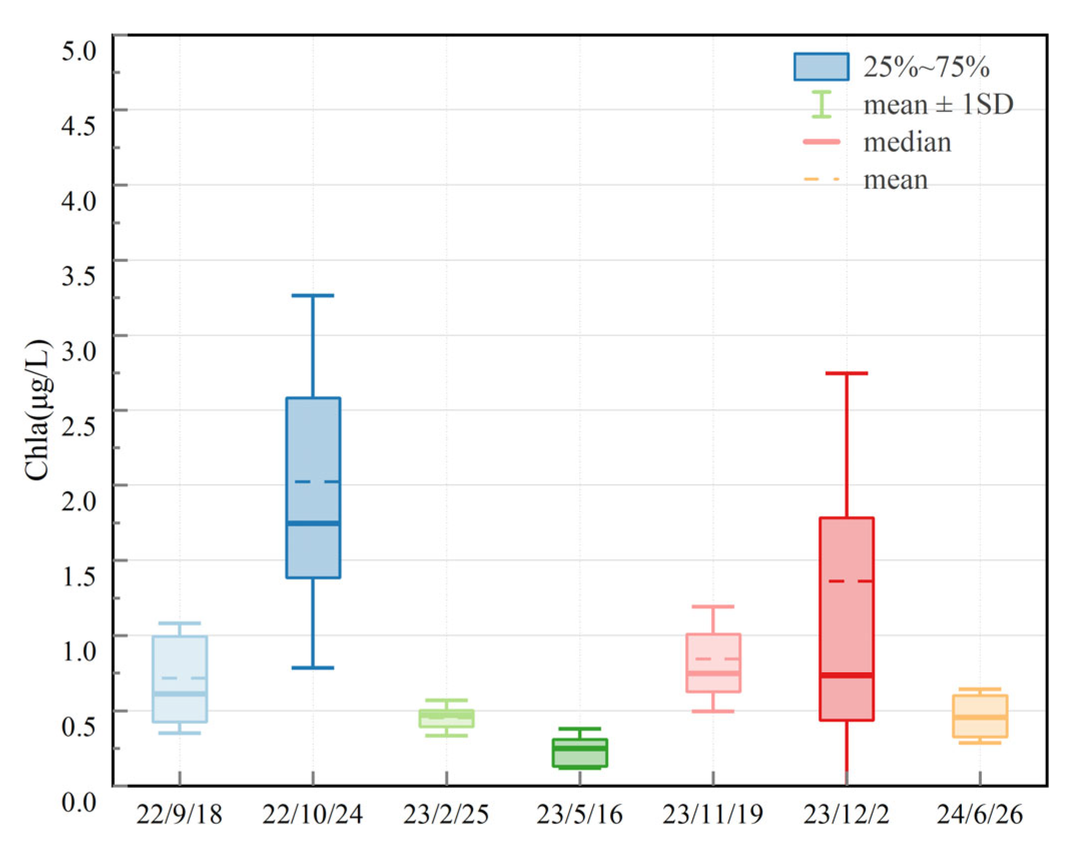
The experimental team also collected in situ water quality data during ASD data acquisition and measured the Chl-a concentration at a depth of approximately 10 cm below the water surface at 127 sampling points using an EXO multi-parameter water quality sonde. Twenty-five measurements were taken at each sampling point, and the average value of all measurements was taken. The EXO water quality sonde measures the Chl-a concentration in a water body using fluorescence photometry and can obtain Chl-a concentration data at a 0.01 μg/L resolution within the range of 0–400 μg/L. The collected Chl-a concentration data is shown in Figure 3.

2.2.3. Collection of UAV Hypercritical Images

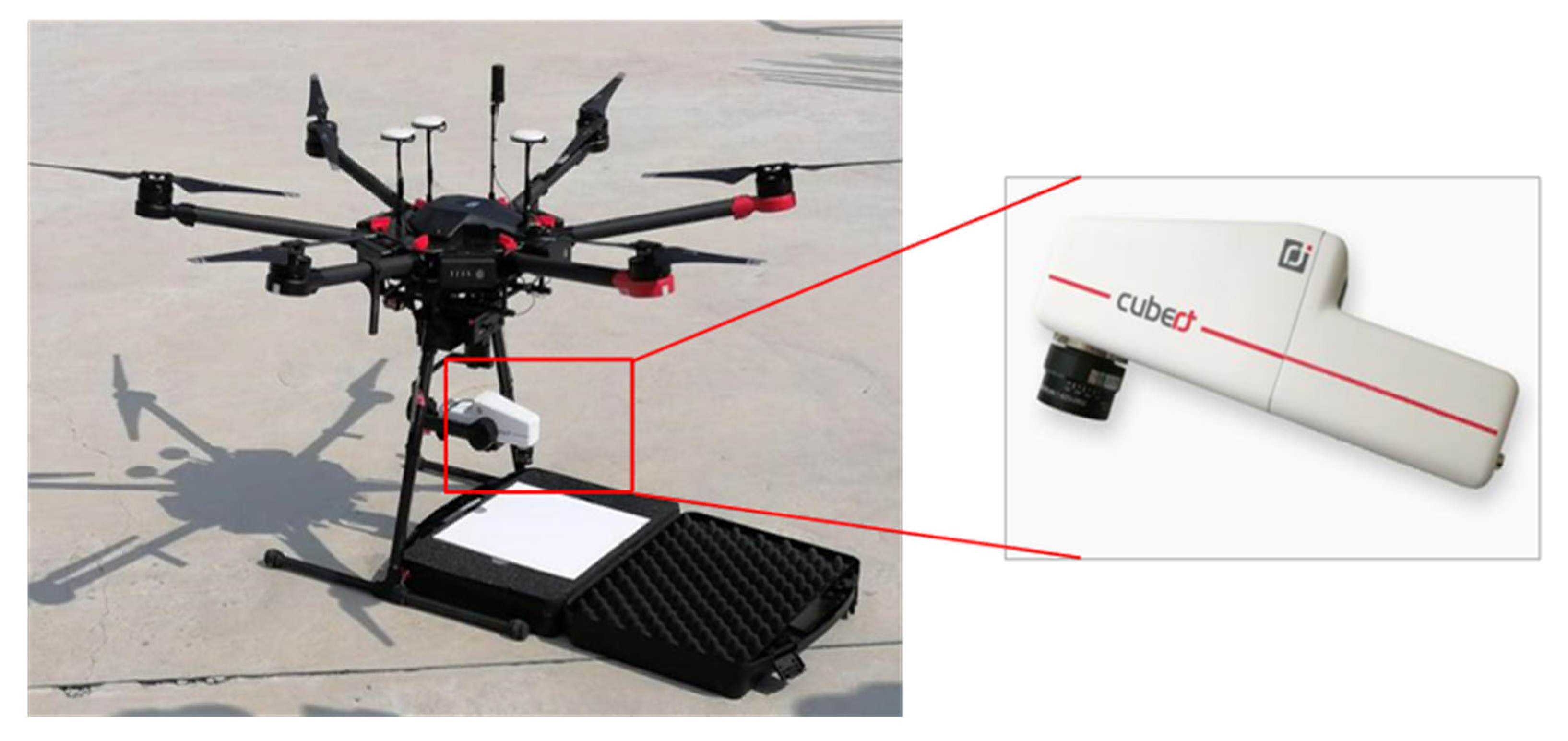
The UAV hyperspectral images for this study were collected using a DJI M600 Pro hexacopter (Made in China) shown in Figure 4 with a 1668 × 1518 × 727 mm payload platform, a maximum speed of 65 km/h, a full-load weight of 6 kg, a recommended flight altitude of no more than 300 m, a maximum pitch angle of 25°, flight endurance of about 15 min, and a maximum wind speed resistance of 8 m/s. The DJI M600 Pro hexacopter is capable of hovering over the water surface for observation and is equipped with a visual positioning system and a forward obstacle detection system.
During data collection from the research vessel, hyperspectral images of the water body in the study area were collected using an UAV equipped with a Cubert Utilities S185 hyperspectral imager. The Cubert S185 hyperspectral imager integrated in the system uses the frame-type hyperspectral imaging technology, integrates accurate hyperspectral data acquisition and fast snapshot imaging, and can synchronously acquire imaging data from all spectral channels at snapshot speed, produce images with dimensions of 1000 px × 1000 px, and effectively balance the temporal resolution, spatial resolution, and spectral resolution. Unlike traditional pushbroom scanners, the Cubert S185 hyperspectral imager adopts an optical path design without moving parts and can acquire a complete hyperspectral image within 1/1000 s, and with its compact design, it weighs only 490 g and is particularly suitable for UAV-based mobile applications for rapid measurement. Some of its performance parameters are given in Table 2.
UAV imaging was carried out at an altitude of about 240 m in clear-sky, cloudless, and windless conditions at 12:20 on 2 December 2023, when the solar azimuth was about 189° and the solar altitude angle was about 59°. The flight plan fully considered the interference of solar glares, and five flight strips were designed, covering more than 150 hm2 of calm water surface.
(1)
Radiometric calibration
Before aerial imaging, the team prepared five Spectralon standard diffuse reflectance panels (2% to 98% reflectance) for radiometric calibration, assuming linearity between sensor response (DN values) and panel reflectance [16]. Calibration was performed automatically in CubeExport software (version 2.6.33561) via piecewise linear mapping.
(2)
Image stitching
Based on Alejandro et al. [24], intra-strip stitching was performed using structural similarity with metadata (GPS, timestamps, camera params, and overlap). Inter-strip used spectral matching for similarity, then geometric transforms. Georeferencing matched Sentinel-2 imagery, with accuracy within one pixel (<10 m).
(3)
Noise filtering
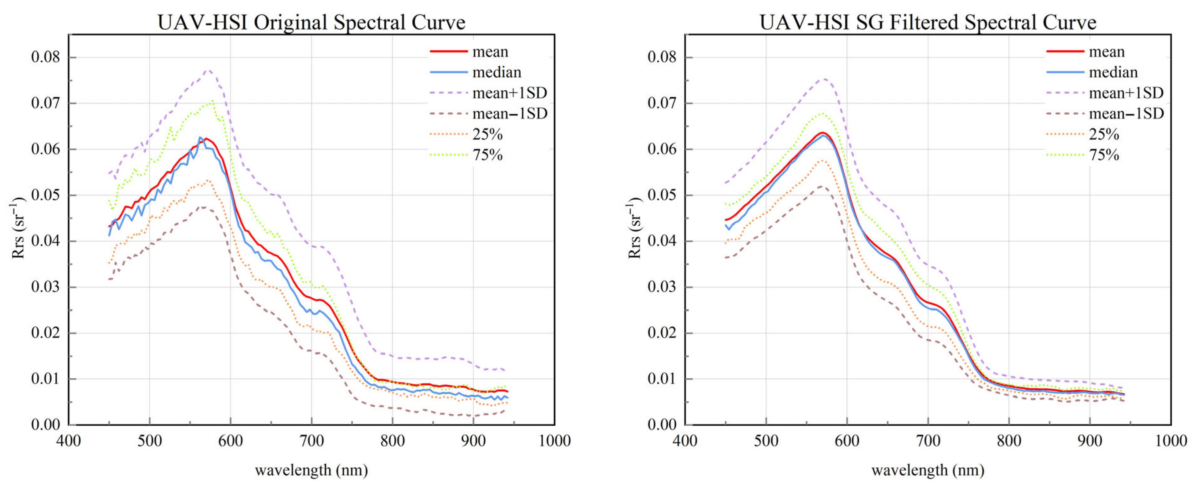
Noise in UAV sensor data mainly consists of spectral noise and spatial noise. Spectral noise is usually caused by spectral artifacts produced due to the sensor’s response capability issues and errors in image stitching [25], and it is mainly concentrated in the ultraviolet and infrared bands. In this study, 125 bands from the 6th channel to the 130th channel were retained, and a Savitzky–Golay filter was used to eliminate spectral noise [26] and improve SNR. Spatial noise mainly originates from the noise pixels produced by environmental factors and interference, such as wave surface foam and electromagnetic noise, in the imaging process. In this study, noise pixels were identified and removed through Lee filtering [27]. The spectral curves of the original and filtered images at the measured point are shown in Figure 5. The true color image of the filtered UAV hyperspectral image (UAV-HSI) is shown in Figure 1.

2.2.4. Sentinel-2 Multispectral Images

The S2 data used in this study comes from the L1C product of the multispectral images (MSI) captured by Sentinel-2B across the study area on 2 December 2023, provided by the European Space Agency (https://browser.dataspace.copernicus.eu/, accessed on 5 September 2024) (hereinafter referred to as S2). The L2A data has been geometrically corrected and atmospherically corrected by Sen2Cor. The true color image after resampling to 10 m resolution in SNAP is shown in Figure 1. Pixels with modified normalized difference water index (MNDWI) [28] values greater than 0.5 were extracted as the pixels representing the water body.

2.3. Matching Method of “Ground–Aerial–Satellite” Data

In this experiment, “Ground–Aerial–Satellite” data exhibit significant differences in spectral and spatial resolution due to variations in sensor configurations. The session introduced three main parts to keep spectral and spatial resolutions matched, including equivalent spectral transform, “Aerial–Satellite” spatial matching, and “Ground–Aerial” spatial matching.

2.3.1. “Ground–Aerial–Satellite” Spectral Matching by Equivalent Transform

Since the band settings of ASD, UAV, and Sentinel-2 (S2) data are inconsistent, in order to apply the Chl-a inversion model based on ASD data to satellite remote sensing data, this study employed the spectral response function of the Sentinel-2B satellite to transform ASD and UAV data into equivalent satellite remote sensing reflectance, thereby ensuring spectral consistency across multi-scale remote sensing data [29]. The calculation formula is as follows:
R = λ 1 λ 2 S λ r λ d λ λ 1 λ 2 S λ d λ
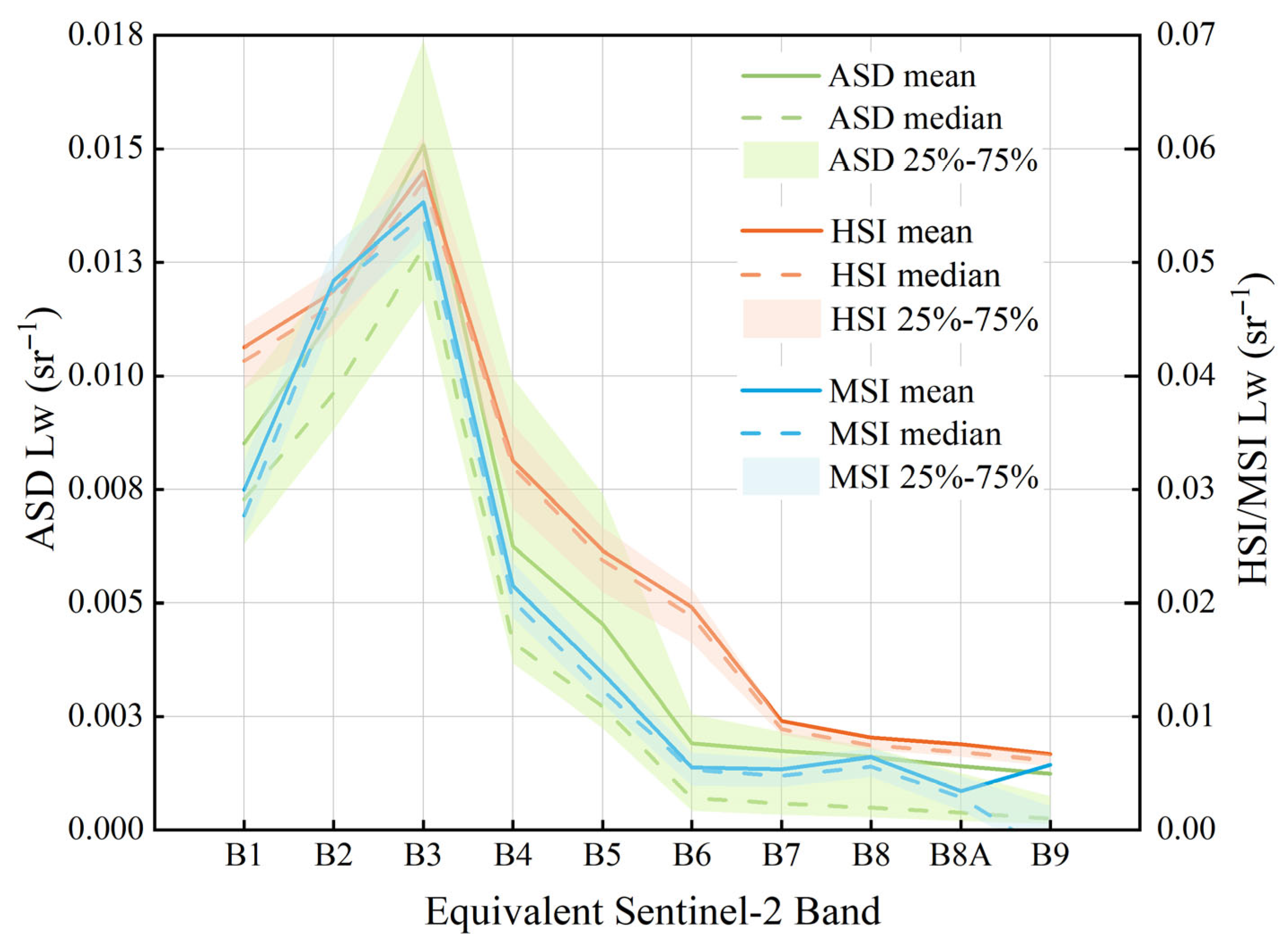
where λ is the wavelength, expressed in nm; S ( λ ) is the spectral response of the satellite sensor in this band; r ( λ ) is the remote-sensing reflectance of the input data; and R is the calculated equivalent satellite remote-sensing reflectance. The spectral response ranges of ASD and UAV data correspond to 10 bands from B1 to B9 of Sentinel-2B data. The calculated remote-sensing reflectance values of the three types of data are shown in Figure 6.

2.3.2. “Aeria–-Satellite” Spatial Matching by Average Pooling

The spatial resolution of UAV data (1 m) is significantly lower than that of S2 data (10–60 m). To ensure spatial consistency, partition grids were constructed according to the geometry of S2 image pixels with 10 m spatial resolution, and after outliers were removed, average pooling was performed on UAV image pixels at a spatial resolution of 10 m.

2.3.3. “Ground–Aerial” Spatial Matching by MPP

Su’s experiment [23] demonstrated that estimating the remote-sensing reflectance at the measuring point by averaging or resampling neighboring pixels is highly unreliable. In order to build a robust model for linear regression of remote sensing images against water quality parameters, Su et al. proposed an enumeration-based Pixel-by-Pixel Matching (MPP) algorithm to find the set of pixels for which the optimal regression equation for water quality parameters at the measuring point can be established and the most reliable inversion equation can be obtained [23]. The MPP algorithm has achieved good results, and its effectiveness has been verified by multiple independent research teams [30,31]. Therefore, in this study, MPP is employed to achieve “Ground–Aerial” spatial matching.

2.4. GASAC

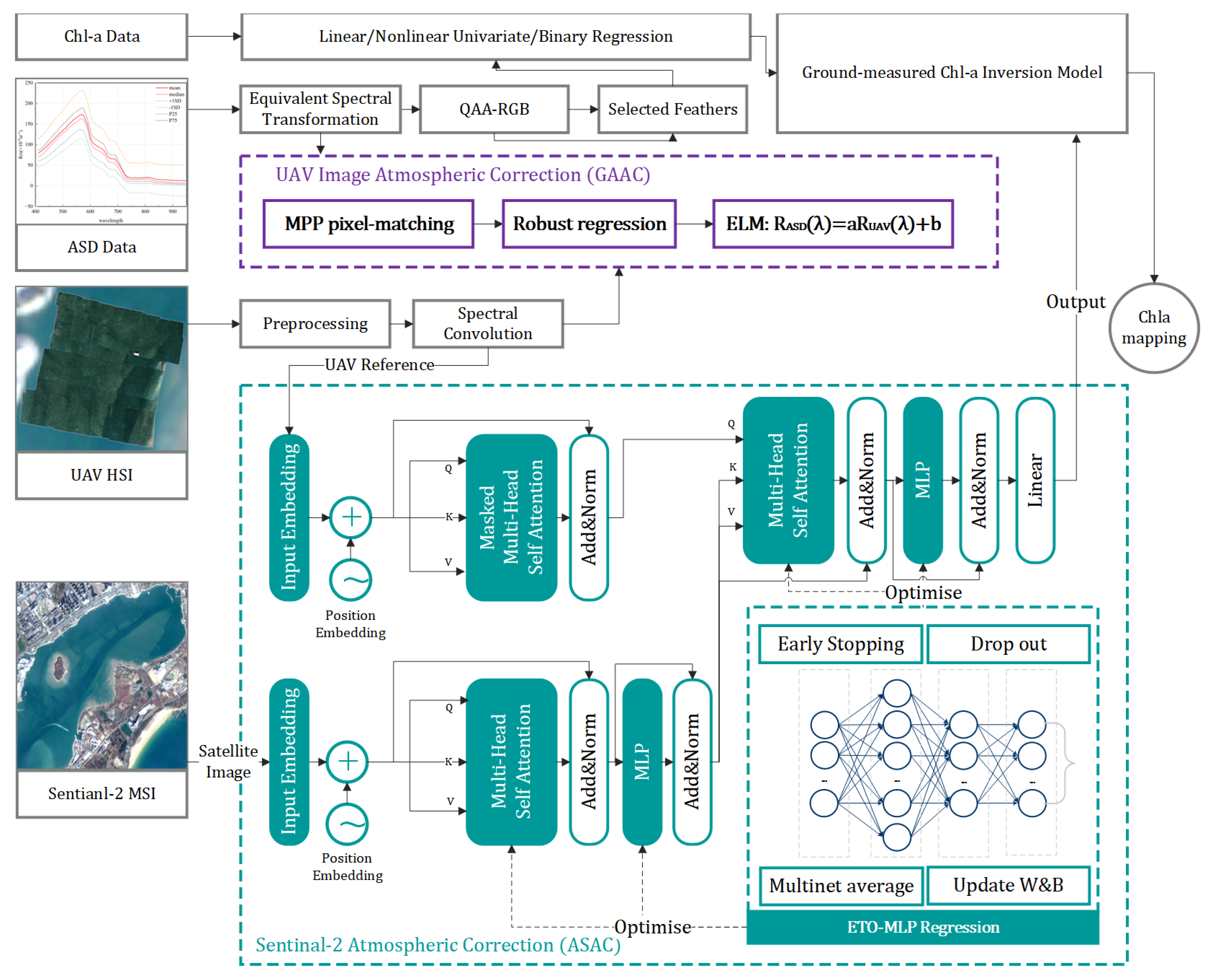
In this study, based on the equivalent remote sensing reflectance derived from three types of remote sensing data, the ASD data were used as the true reference. A Pixel-by-Pixel Matching (MPP) method combined with the Empirical Line Model (ELM) [16,32] was employed to perform ground–aerial atmospheric correction (GAAC) for UAV data. The corrected UAV data then served as the reference for fitting atmospheric correction of Sentinel-2B L1C image in bands B1–B9 using a Transformer-based model, thereby constructing the ASAC. The GASAC results of the satellite imagery were evaluated for accuracy across multiple control groups. The corrected satellite data were subsequently applied to a Chl-a inversion model built from ASD data to map chlorophyll-a concentrations from Sentinel-2 imagery across different experimental dates in the study area. The detailed research workflow is clearly illustrated in Figure 7.

2.4.1. GAAC by MPP-ELM

Although UAVs fly at low altitudes and their sensors are subject to less atmospheric interference, there are significant differences between UAV remote sensing images and measured data due to interference from factors such as the presence of near-ground aerosols, specular reflection, and calibration errors. Therefore, it is necessary to build an effective GAAC model [33].
In ocean color remote sensing, the radiation signal L s e n s o r λ received by the sensor can be decomposed into the sum of the water-leaving radiance ρ w after path radiance and atmospheric attenuation and the specular reflection part L r . Its mathematical model can be expressed as [32]:
L s e n s o r λ = L R λ + L A λ + T λ , θ L r λ + t λ , θ ρ w ( λ )
where L R is the Rayleigh scattering radiance of atmospheric molecules and L A λ is the aerosol scattering radiance, both of which can be attributed to the path radiance part; T λ , θ is the direct atmospheric transmittance, and t λ , θ is the diffuse transmittance. Since the atmospheric properties at the water surface are stable and homogeneous, t λ , θ can usually be considered a constant. Without considering the effect of specular reflection, radiative transfer is a linear process, and the corresponding atmospheric correction method is called the Empirical Line Method (ELM), which has been widely used in atmospheric correction of remote sensing data, especially UAV remote sensing data [34].
Atmospheric correction of low-altitude ocean color remote sensing images (UAV images) based on in situ measurements (ASD data) was achieved by combining the MPP and ELM models band by band. The MPP search range was set to match the georeferencing accuracy of the UAV imagery. The input variables were the ten equivalent Sentinel-2 band reflectance values from the UAV image obtained after MPP, and the response variables were the corresponding equivalent reflectance values from the ASD data.
Given the small-sample linear regression context of this study, the impact of outliers can be critical. Therefore, a robust regression method was adopted, which iteratively adjusts weights to gradually approach the optimal solution and resist the influence of extreme values [35]. The entire modeling process was implemented in MATLAB (version 2024b), with robust regression performed using MATLAB’s default robust fitting settings.

2.4.2. ASAC by Transformer

UAV images processed through GAAC can be approximately regarded as ideal atmospheric correction results for satellite-borne sensors, making it feasible to construct correction models via empirical regression. MLP (Multi-Layer Perceptron) possesses strong nonlinear fitting capabilities, often outperforms other regression models such as linear regression, random forests, and support vector machines in regression tasks [36], and has been widely applied in the field of ocean color remote sensing [37,38]. In this section, an ETO (Exponential-Trigonometric Optimization)-Transformer-MLP model (hereafter referred to as ETMNet) is constructed by using MLP as the base learner, incorporating Transformer attention mechanisms, and optimizing with the ETO algorithm. ETMNet fits the post-GAAC UAV data using temporally and spectrally consistent Sentinel-2 data to achieve ASAC.
(1)
Data preparation
The input data includes the remote-sensing reflectance values of the original S2 image in each band (B1 to B9), along with pixel location and central wavelength information within the UAV imaging area. The target data were the UAV image reflectance values processed through GAAC, spectral harmonization, and average pooling, resulting in a total of 10,980 valid samples. To evaluate the true performance of the ASAC model, S2 pixels located near the sampling centers were selected as the test set. The remaining data were stratified by reflectance values, from which 10% were randomly selected as a cross-validation set, and the remaining 90% were used as the training set, resulting in an approximate dataset split ratio of 7:1.5:1.5 for training, validation, and testing sets.
(2)
ETO algorithm
Different network parameters, initial weights, and biases in MLP often have a decisive impact on the results of MLP training. The usual practice is to use an optimizer to perform a hyperparameter search and find the optimal solution set.
The ETO algorithm proposed by Luan et al. [39] was employed in this study, which is a metaheuristic optimization algorithm that integrates exponential and trigonometric functions and improves search efficiency by dynamically balancing global exploration and local exploitation. Its core steps and equations are described below.
(a)
Initialization phase: Randomly generate an initial population within the upper and lower bounds as follows:
i i j = U p j L o w j × r a n d + L o w j
where r a n d is a uniformly distributed random number over the interval [ 0 ,   1 ] and U p j and L o w j are the upper and lower bounds of the jth dimension.
(b)
Constrained Exploration: Dynamically adjust the search space to balance computational efficiency and solution quality:
C E i + 1 = f l o o r 2 2 × t × M a x I t e r C E i × a + C E i
C E i = f l o o r 1 + M a x I t e r b
where t is the current number of iterations, M a x I t e r is the maximum number of iterations, floor represents rounding down, and the two adjustment coefficients a and b are equal to 4.6 and 1.55, respectively. The value of C E i is determined by Equation (5), while C E i + 1 represents the iteration counts that initiate the present and subsequent constrained exploration approaches [39]. After the constrained exploration strategy is implemented, the upper and lower bounds of the search space will be updated.
(c)
Exponential-trigonometric optimization: During the development phase, the ETO algorithm will focus on local perturbations near the determined optimal solution to further improve the quality of the solution:
X t + 1 i j = X t i j + c × r a n d × a 2 × X j b e s t X t i j
c = exp tan d 1 d 2
d 1 = 0.1 × exp 0.01 × t × cos 0.5 × M a x I t e r × 1 t M a x I t e r
d 2 = 0.1 × exp 0.01 × t × cos 0.5 × M a x I t e r × 1 t M a x I t e r
In this context, the j th position of the most optimal solution discovered thus far is denoted by X j b e s t . X t i j and X t + 1 i j represent the j th positions of the i th solution during the current t and subsequent t + 1 iterations, respectively. The parameters d 1 and d 2 are employed to construct the novel exploration space. This exploration space will progressively contract as the optimization process advances, thereby enhancing the precision and velocity of convergence. In the equation for calculating the coefficient c , the exponential and trigonometric functions are intricately combined, which enhances the search process and improves the optimal location update mechanism.
(d)
Changeover Method: The ETO algorithm uses a CM to enable flexible changeover between exploration and exploitation. When the value of C M > 1 , ETO is in the exploration mode. Conversely, when C M < 1 , ETO shifts to the exploitation mode, thus ensuring the exploration and exploitation of the entire search domain while avoiding getting stuck in local optima.
C M = 0.01 × r a n d × s q r t t M a x I t e r t a n d 1 d 2
In summary, the ETO algorithm involves a very small number of parameters to be tuned and can effectively improve the convergence speed and accuracy by dynamically updating particle locations and exploration and exploitation strategies through various strategies, thereby assigning the optimal initial bias and weight to each neuron and connection line.
(3)
Optimization and training strategy of ETMNet
The training strategy has a decisive impact on both the training speed and accuracy of deep networks. In this experiment, the Scaled Conjugate Gradient (SCG) algorithm—known for balancing efficiency and performance—was first adopted as the gradient descent method [40]. To prevent overfitting, techniques such as Early Stopping, Dropout, and cross-validation were employed [41,42]. Additionally, an ensemble learning approach was used, in which multiple identical neural networks were trained in parallel and their outputs averaged, significantly reducing the variance component of the prediction error [36].
With the aid of the ETO algorithm, optimal network design parameters suited to the task were obtained. A lightweight Transformer architecture was designed for this study (as shown in Figure 7). Based on commonly used configurations in similar research and considering computational constraints, the optimization objective was set as the mean squared error (MSE) on the cross-validation set. The optimal parameter solution set was searched using an initial population of 50 individuals over 500 iterations. The parameters include the number of attention heads in the Transformer, the embedding dimension of the encoder, the number of neurons in the hidden layers, initial weights and biases of each neuron, the number of early stopping rounds, and the target error threshold. These settings were tailored to the characteristics of areal AC data, aiming to improve both model fitting and generalization capabilities. The ASAC results of ETMNet are presented in Section 3.2.

2.5. Verifying AC Accuracy by Inverting Chl-a Concentration

The accuracy of atmospheric correction directly affects the accuracy of water quality testing, and water quality testing is a core task in ocean color remote sensing. Therefore, it is necessary to further verify the quality of atmospheric correction through water quality testing. The Chl-a concentration is an important parameter in water quality testing that reveals the eutrophication levels of water bodies [43]. In this study, Chl-a concentration inversion was performed to evaluate the effect of atmospheric correction and demonstrate the practical value of GASAC. In the following paragraphs, the procedure for building the optimal Chl-a concentration inversion model based on ASD data will be described from two aspects, namely, the combination and selection of features and model building.

2.5.1. Feature Selection and Combination for Chl-a Concentration Inversion

In ocean color remote sensing, chlorophyll-a (Chl-a) concentration inversion models are commonly constructed through regression using combinations of multi-band water-leaving radiance or inherent optical properties (IOPs) derived from these radiances via the QAA algorithm [44]. In this study, equivalent-calculated ASD data for each band, along with the IOPs derived from these data using the QAA-RGB algorithm [29], were systematically combined. Based on the formulas provided in Table 3, a total of 3070 candidate features were generated, including single-band, two-band, three-band, and four-band combinations. Each feature was evaluated by calculating its Pearson correlation coefficient and significance level with Chl-a concentration. As a result, 41 spectral combination features with correlation coefficients greater than 0.6 and p-values ≤ 0.05 were identified, along with 8 valid IOP-based combination features.

2.5.2. Chl-a Concentration Inversion Model Building

Linear regression models are the most commonly used empirical models in ocean color remote sensing. However, due to interference from optically active components [45] and pigment encapsulation [46], there is a nonlinear relationship between optical properties and the Chl-a concentration. Studies have shown that the inversion accuracy can be effectively improved by using the log transformation and fitting quadratic and exponential functions [44]. Univariate fitting of the spectral features obtained in Section 2.5.1 was performed on an item-by-item basis using the model given in Table 4, and binary fitting with the IOPs [47] was performed using the robust regression method described in Section 2.4.1.

2.6. Model Accuracy Metrics

This experiment primarily employed four metrics— R 2 , R M S E , M A E , and M A P E —to evaluate the performance of the models. These metrics were used to assess the atmospheric correction accuracy of the GASAC model in Section 2.4 based on in situ measurements, the accuracy of the Chl-a inversion model in Section 2.5.2, and the prediction accuracy of inversion models under different GAC strategies presented in Section 2.6. The definitions of the four metrics are provided below. To improve data readability, all RMSE and MAE values reported in this study are scaled by a factor of 10,000, with units expressed as 10−4sr−1.
R 2 = 1 1 n y i y i ^ 2 1 n y i y i ¯ 2
R M S E = 1 n 1 n y i y i ^ 2
M A E = 1 n 1 n y i y i ^
M A P E = 1 n 1 n y i y i ^ y i × 100 %

3. Results

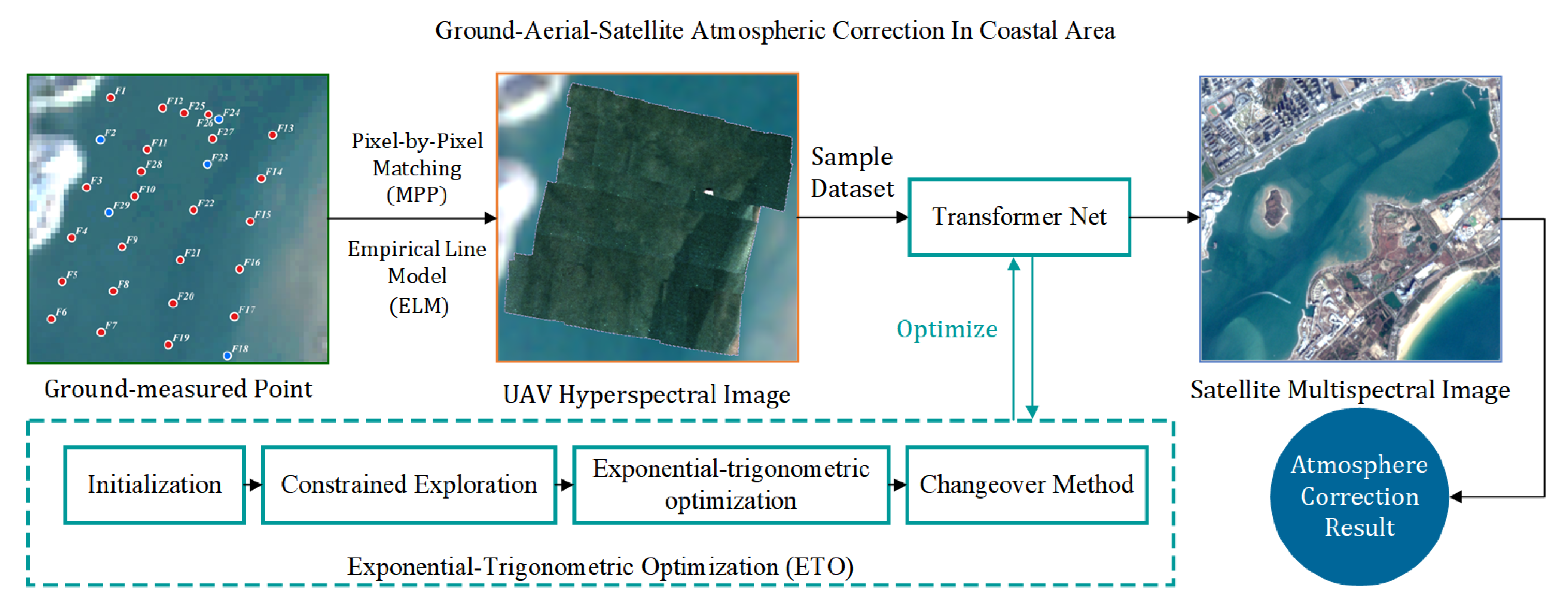
This chapter first presents the GAAC accuracy of UAV data by comparing it with in situ ASD measurements. Next, the ASAC accuracy of Sentinel-2 (S2) data is demonstrated by a comparison with spectrally harmonized UAV data. In the third part, the necessity and advantages of the stepwise GASAC approach are illustrated by comparing the atmospheric correction results of S2 data under three different GAC strategies—GAAC, GSAC, and GASAC—at the sampling points. Finally, the effectiveness of the proposed method is validated by comparing the inversion accuracy of Chl-a concentration models using the three different atmospheric correction results. The main process of GASAC is shown in Figure 8.

3.1. Evaluation of GAAC Results

However, the MPP algorithm is very complex. For m sampling points, each with a sampling range of n × n pixels, a total of n 2 m computations are required, and the computation time increases exponentially with the number of sampling points. Fortunately, UAVs fly in small ranges and can achieve fast imaging; within a short time, aerosols in a small area are approximately evenly distributed, and the atmospheric effects tend to be the same at different points. For reference, the area of the study region is approximately 17 km2, which is considered sufficient for the application of our method under the assumption of atmospheric homogeneity based on observed atmospheric data. Therefore, a small number of representative sampling points with typical water characteristics can be selected as the training set [23].
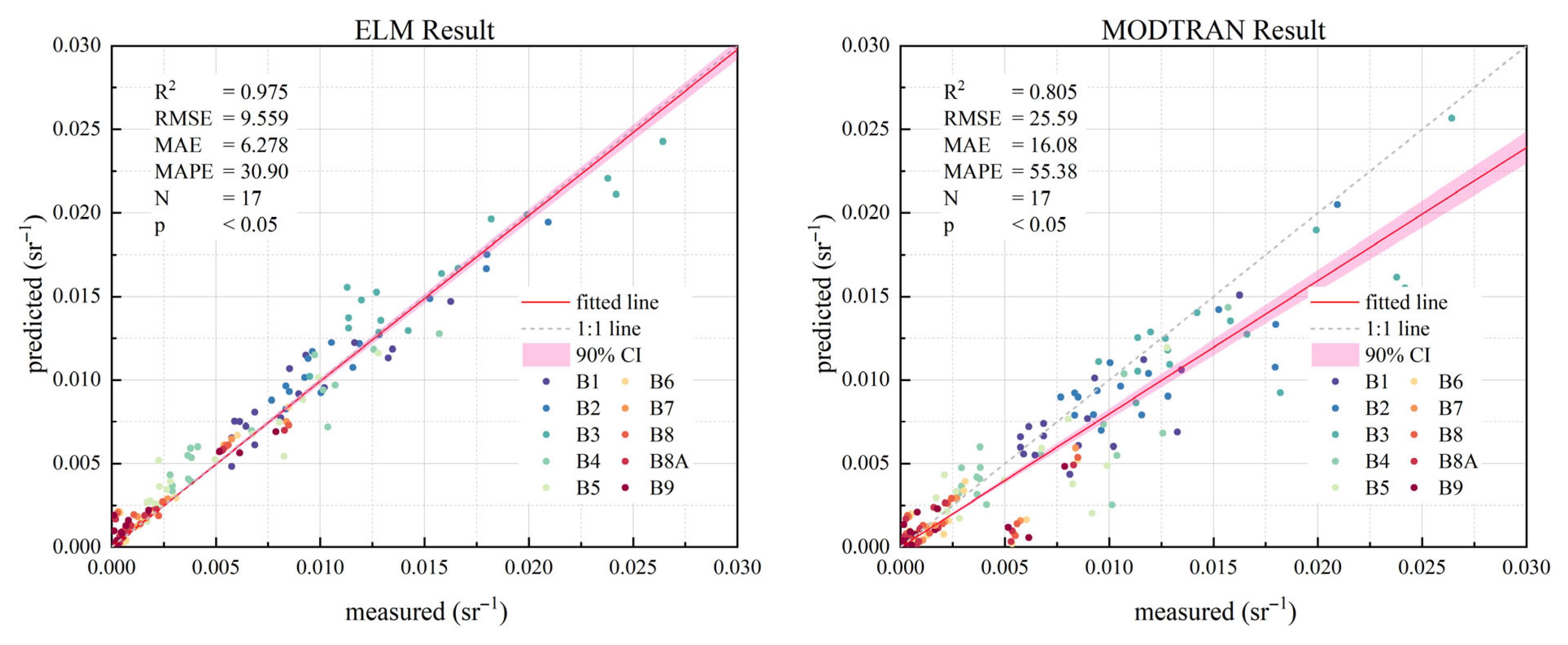
Based on the measured equivalent water-leaving radiance, this experiment applied spatial multivariate clustering to determine the water type associated with each sampling point. The number of clusters was determined using the elbow method [48], and the five representative sampling points (F2, F18, F23, F24, and F29) closest to the cluster centers were selected as the training set for aerial-to-satellite atmospheric correction. The remaining points were used as the test set. The ELM model obtained in Section 2.4.1 was applied to the MPP-matched pixels of the test sampling points. At the same time, a control group using a commonly adopted physical correction method for low-altitude water imaging was set up for comparison [49]. The physical method used the MODTRAN 5 model, with input parameters including ground-observed meteorological data (temperature, pressure, and humidity) and imaging geometry (observation height, viewing angle, solar azimuth angle, and solar elevation angle). The aerosol model was set as the maritime model, and other parameters followed the model’s default settings to obtain atmospheric correction parameters [50]. The atmospheric correction accuracy of the two methods on the validation set is shown in Figure 9.

3.2. Evaluation of ASAC Results

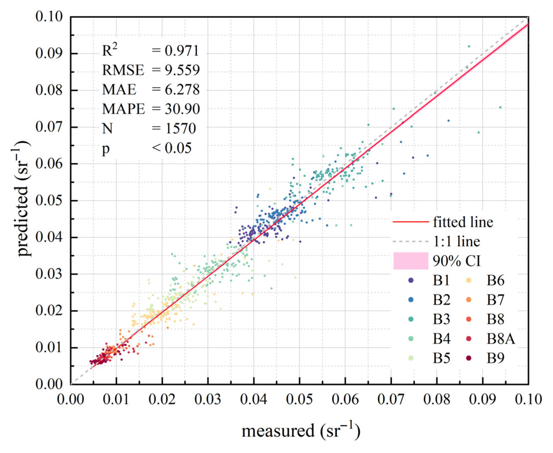
The prediction results of the ETMNet model obtained in Section 2.4.2 on the test set are shown in Figure 10, where the horizontal axis represents the spectrally harmonized UAV reflectance, and the vertical axis represents the predicted reflectance output by ETMNet from the input S2 data.
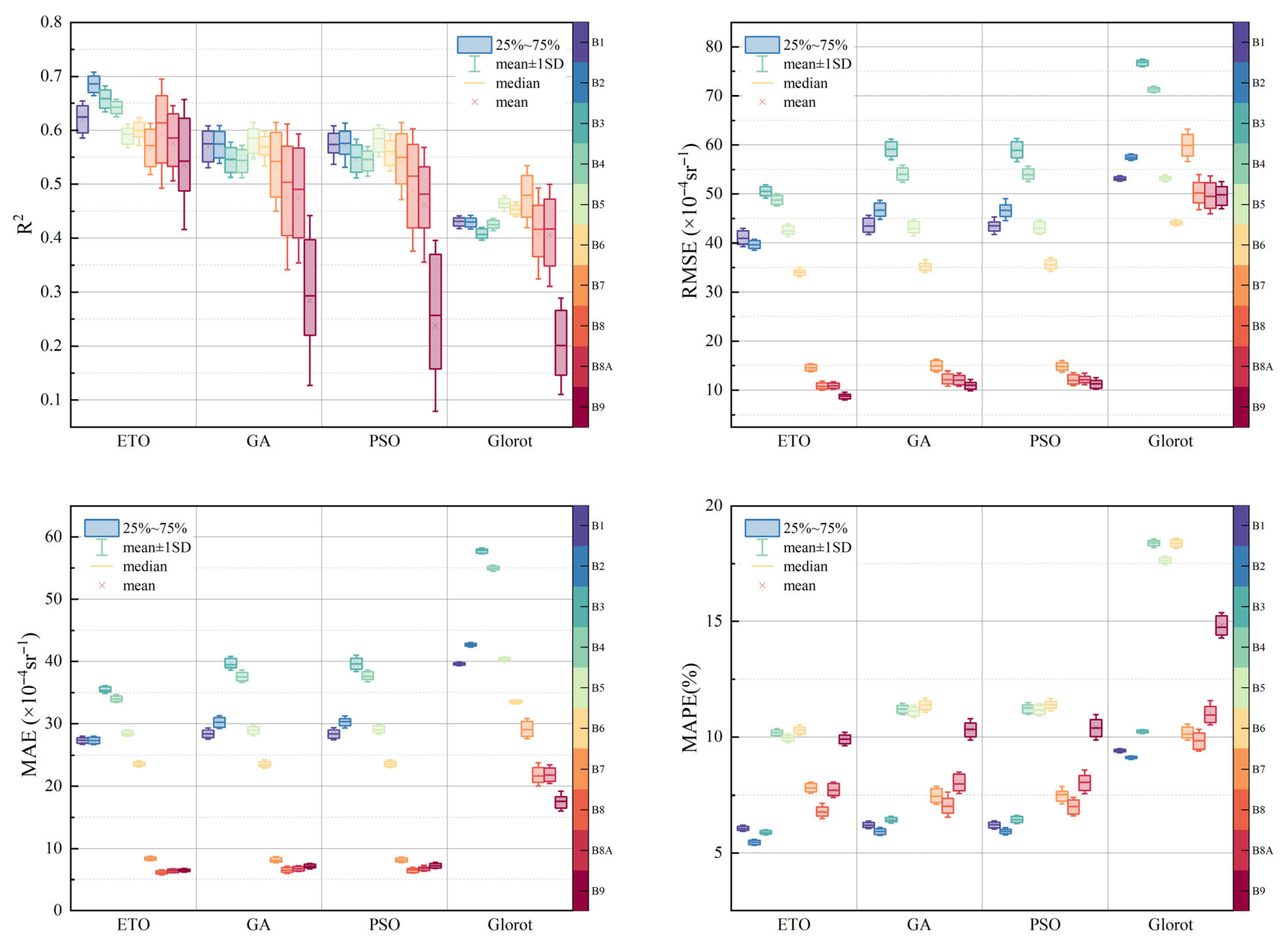
To further verify the effectiveness and superiority of the ETO optimizer within ETMNet, this study introduced two classic optimization algorithms—Particle Swarm Optimization (PSO) [51] and Genetic Algorithm (GA) [52]—as control groups, using the same optimization strategy as in Section 2.4.2. Additionally, a non-optimization control group was set up, in which the network parameters were randomly initialized using the Glorot initialization strategy [53]. Due to the inherent randomness of the ETMNet training process, each group of optimization results was trained 100 times to better observe and compare the stability and performance of the solutions and enhance the reliability of the results. The training results under the four evaluation metrics—R2, RMSE, MAE, and MAPE—are presented in the form of box plots in Figure 11.
The figure compares the performance of four optimizers: ETO, GA, PSO, and Glorot. ETO demonstrates superior solution quality with lower average MAE, RMSE, and MAPE values. Additionally, the shorter box lengths for ETO indicate greater solution stability. In contrast, Glorot, lacking iterative optimization, performs relatively poorly. The results of the above experiments demonstrate the advantages of the ETO optimizer.

3.3. Comparison of Correction Results from the Three GAC Strategies

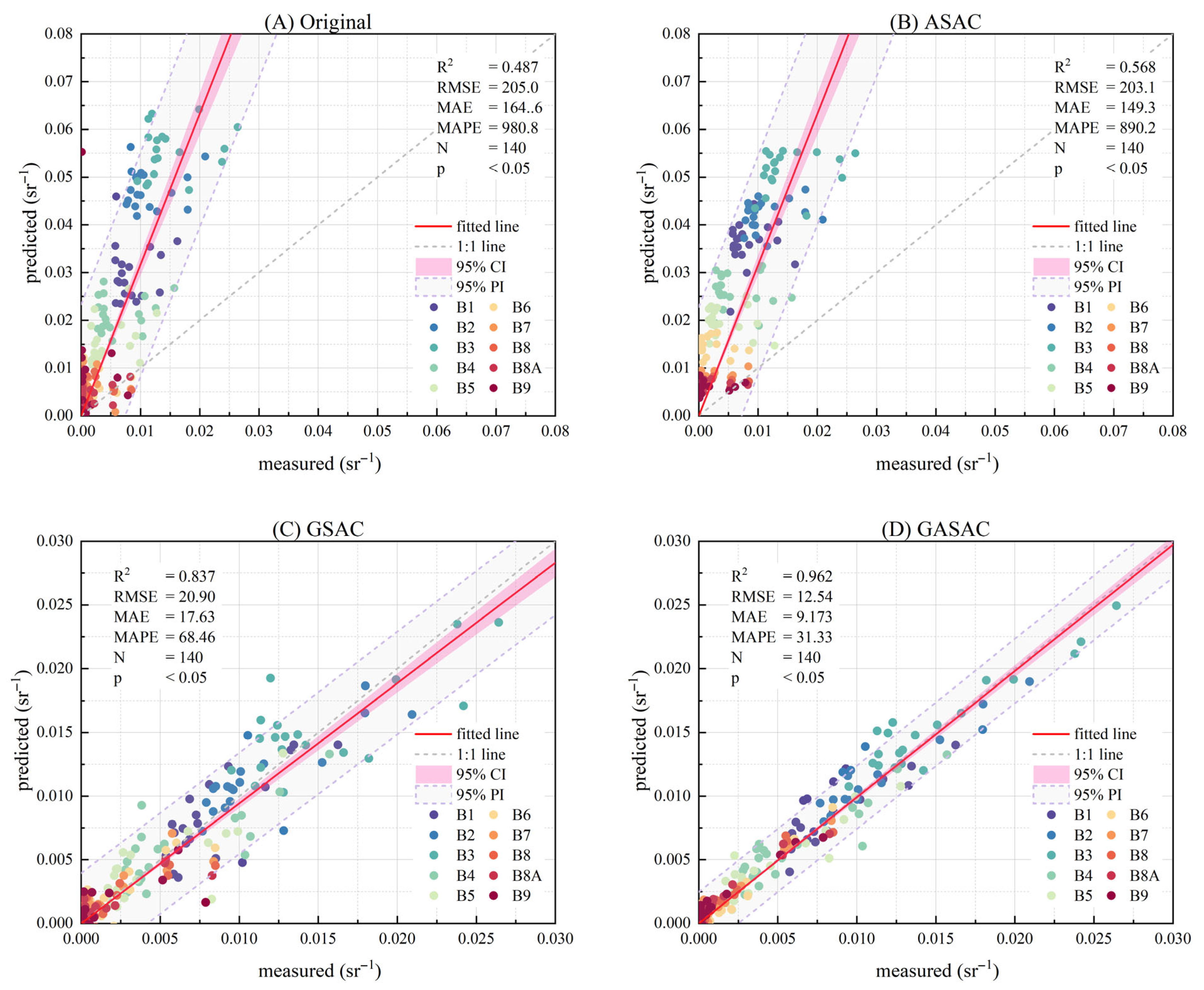
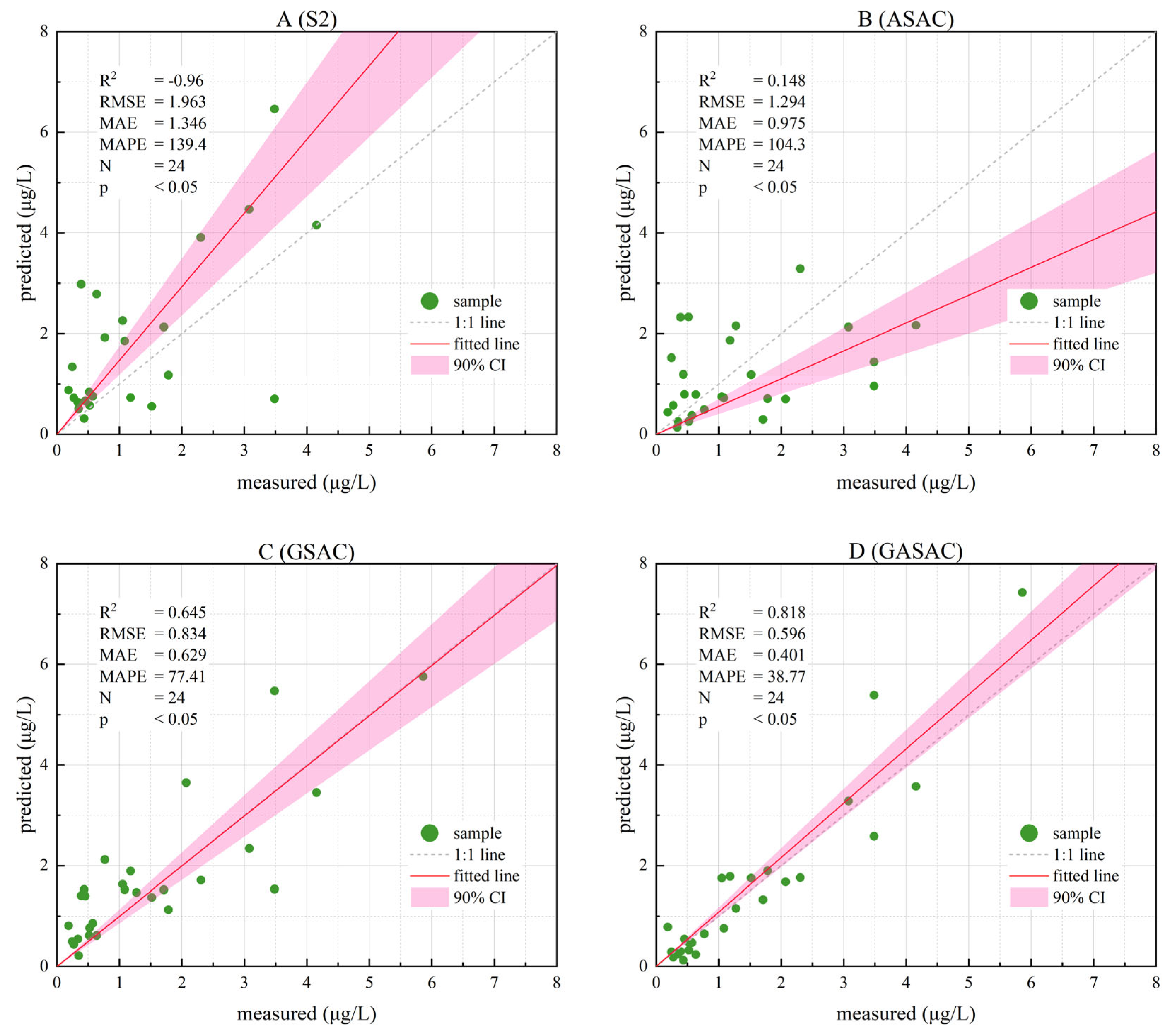
Four ablation experiments (Groups A–D) were designed to verify the necessity and superiority of GASAC. Group A used the original S2 data, representing the atmospheric correction results from classical physical methods. Group B used S2 data after ASAC without applying GAAC to assess the impact of near-surface atmosphere on UAV data. Group C constructed a GSAC model by directly linking S2 data with in situ ASD measurements using the method described in Section 2.4.1 to evaluate the necessity of introducing UAV data. Group D followed the full stepwise GASAC procedure.
As Figure 12 shows, among the four atmospheric correction methods, the accuracy of Group B is significantly lower than that of Groups C and D, indicating that incorporating ground-measured data for GAAC is essential. The atmospheric effects caused by near-surface aerosols remain non-negligible but can be effectively removed using MPP-ELM under reasonable pixel matching. The GSAC approach used in Group C can partially eliminate atmospheric effects in satellite data, but its correction accuracy is limited by both the sample size and the fitting capacity of the mathematical model, resulting in a lower performance compared to Group D. Group D achieved the highest correction accuracy, demonstrating clear advantages. These results indicate that constructing a stepwise GASAC model by integrating multi-scale data can effectively improve atmospheric correction accuracy.
The analysis above shows that, compared with the GSAC and ASAC methods involving two data sources, the GASAC model based on three types of data has significant advantages and is a feasible method for high-precision atmospheric correction of satellite data.

3.4. Impact of Atmospheric Correction on Chl-a Concentration Inversion

In this section, the results produced by the method described in Section 2.5 are discussed, and the optimal Chl-a concentration inversion model is built using the selected features and applied to four sets of atmospheric correction results to further demonstrate the impact of atmospheric correction accuracy on water quality testing and the practical significance of high-precision atmospheric correction.

3.4.1. Building of the Chl-a Concentration Inversion Model Based on Measured Spectra

In ocean color remote sensing, the accuracy of atmospheric correction directly determines the inversion accuracy. ASD data is of high quality and is not affected by the atmosphere. Therefore, such data is ideal for the inversion of water quality parameters. An accurate Chl-a concentration inversion model can be obtained through simple regression and fitting. The model is highly sensitive to input data and can significantly reflect the impact of atmospheric correction on the inversion of water quality parameters. The process of obtaining the optimal Chl-a concentration inversion model using the method described in Section 2.5 and the related results are described below.
The 27 pieces of data obtained at the S2 imaging time (2 December 2023) are used as the test set, and the remaining 100 pieces of data were used as the training set. Using the method described in Section 2.5.1, a total of 1704 Chl-a concentration inversion models were built, including 392 univariate models and 1312 binary models. The inversion results were evaluated on the test set using the metrics R 2 , R M S E , M A E , and M A P E . Equation (15) is the empirical formula for the model that has produced the best inversion results.
C h l a = 0.028 1 / B 1 1 / B 9 1 / B 4 1 / B 8 A 2 + 107.253 η 2 0.2411 1 / B 1 1 / B 9 1 / B 4 1 / B 8 A 123.046 η + 35.9165
η = 2 2.4 e x p 0.9 0.0096 B 2 B 3 3 + 0.2388 B 2 B 3 2 + 0.5398 B 2 B 3 0.0255
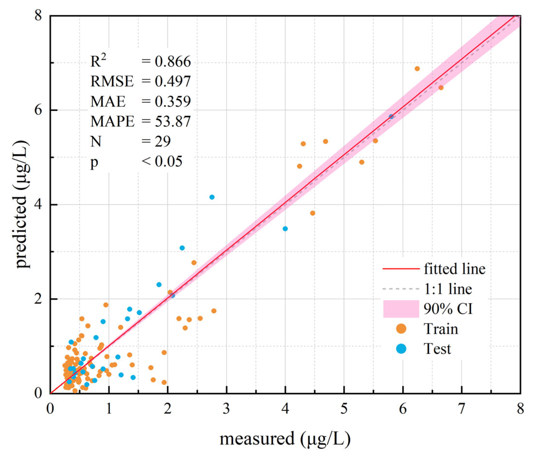
In Equation (15), B 1 B 9 are the water-leaving radiances of the ASD data for the equivalent S2 bands, expressed in s r 1 , and η is the slope of particle backscattering, which represents the degree of dependence of the particle backscattering capability on the wavelength and can be calculated using Equation (16) in QAA-RGB [29]. Figure 13 shows the scatter plot of the results produced by the optimal Chl-a inversion model versus ASD data.
As shown in Figure 13, a high-performance Chl-a concentration inversion model can be obtained through binary quadratic regression and fitting using ASD data in combination with water-leaving radiance data and IOPs. The coefficient of determination ( R 2 ) of the model is close to 0.87. The model has high inversion accuracy, and its quadratic form is sensitive to input parameters. Therefore, it can significantly reflect the impact of atmospheric correction accuracy on water quality testing and demonstrate the practical significance of high-precision atmospheric correction.

3.4.2. Chl-a Concentration Inversion Accuracy of Different GAC Results

The optimal Chl-a concentration inversion model was applied to the four sets of atmospheric correction results obtained in Section 3.3. The relationship between the predicted and measured data is shown in Figure 14.
These inversion results show that the accuracy of Method B and Method C is higher than that of Method A, proving the feasibility of improving the accuracy of atmospheric correction by combining data from other sources. The R 2 value of Method C is 0.4 greater than that of Method B, indicating that it is necessary to perform atmospheric correction based on measured data. Specifically, the R 2 value of Method D (0.82) is greater than that of Method C (0.64), indicating that UAV data plays a crucial role in atmospheric correction and the use of such data can effectively improve the accuracy of atmospheric correction and provide more accurate estimates of the Chl-a concentration.

4. Discussion

In this chapter, we first examine, from a theoretical perspective, the pivotal role of MPP [23] in GAAC for nearshore waters, affirm the validity of the linear assumption for low-altitude atmospheric effects in these environments, and identify future development directions for GAAC. Next, we discuss the data synchronization requirements of ASAC and experimentally assess the potential of ETMNet to extend its applicability to UAV sensors equipped solely with RGB channels. In the third section, we compare the performance of GASAC against baseline models through controlled experiments; concurrently, we explore the temporal generalization capabilities of GASAC, underscore the necessity of collecting synchronized datasets, and present a spatiotemporal analysis of Chl-a concentration distributions in the study area across multiple experimental campaigns.

4.1. Discussion on GAAC

Unfortunately, the academic community currently lacks a universal and accurate atmospheric correction method for low-altitude water color mobile measurement systems. In practical UAV remote sensing applications, empirical methods are often commonly used and efficient choices [33]. However, in aquatic environments, due to the fluidity and high reflectivity of water bodies, it is often difficult to obtain accurately matched pixels for in situ measurement points. This leads to biased atmospheric correction parameters and limits the accuracy and reliability of the models. MPP, as a “point-to-pixel” matching method designed for highly dynamic aquatic environments, was initially proposed based on the assumption of a logarithmic linear relationship between spectral characteristics and in situ water quality parameters. It identifies the optimal pixel set with the best regression performance as the matching result. In this study, based on the linear assumption of near-surface atmospheric effects, MPP was successfully applied to the pixel matching between synchronous in situ water quality points and UAV water color remote sensing imagery, achieving favorable GAAC results.
Both theoretical analysis and experimental results demonstrate that there exists a linear discrepancy between the remote sensing reflectance obtained by UAVs and the above-water radiance required for inversion in this study. According to the radiative transfer equation, this discrepancy mainly arises from atmospheric path radiance and the diffuse transmittance of solar radiation within the water column [32]. During the matching process, MPP effectively reduces environmental interferences—such as mixed pixels, specular reflection, and water movement—by selecting the pixel set with optimal fitting, thereby improving the accuracy and regional applicability of GAAC [23].
To streamline workflows and reduce data acquisition costs, further in-depth research on the water-atmosphere optical mechanism is needed. This will enable the development of low-altitude atmospheric correction methods that do not rely on in situ water spectral measurements while maintaining high accuracy, thereby facilitating reliable above-water radiance retrieval and high-precision water-quality monitoring.

4.2. Discussion on ASAC

This section first discusses the data synchronization requirements of the ASAC method, noting that ASAC requires satellite data with high spatial resolution and a well-aligned spectral channel configuration between the satellite and UAV. Subsequently, experiments are conducted to evaluate the potential of the ASAC method, implemented using ETMNet in this study, to be extended to UAV data equipped with RGB three-channel sensors.

4.2.1. The Synchronization Data Requirements of the ASAC

With respect to spatial resolution, the ASAC model developed in this study is driven by a Transformer architecture, which requires a certain amount of synchronized data to meet the training demands. Due to the limited endurance of UAVs, their imaging area is restricted. Therefore, satellite data must possess high spatial resolution to provide sufficient synchronized data for learning the complex atmospheric effects involved in satellite-to-aerial radiative transfer processes, thereby enabling the construction of a reliable and accurate ASAC model.
In terms of spectral resolution, it is essential that the UAV and satellite exhibit a well-aligned spectral channel configuration, or that the spectral characteristics can be effectively transformed to ensure consistency. The UAV sensor used in this study features high spectral resolution, allowing for the derivation of reliable Sentinel-2 reflectance references through spectral response function-based transformations, thus achieving high ASAC accuracy. For UAVs not equipped with hyperspectral sensors, this study simulated the scenario of an RGB three-channel configuration, and the ASAC modeling results are discussed in detail in Section 4.2.2.
In addition, it is necessary to maintain a minimal imaging time difference and high spatial registration accuracy between UAV and satellite data. This ensures the maximum suppression of environmental noise while preserving the complex atmospheric effects inherent in the satellite-to-aerial radiative transfer process, preventing the ASAC model from inadvertently learning excessive environmental noise.

4.2.2. Generalization Ability Analysis of ETMNet to UAVs Equipped with RGB Channel Sensors

In general, UAV-borne imaging sensors mainly produce RGB images with three channels [34]. In the field of ocean color remote sensing, researchers have developed a wide variety of water quality inversion models based on RGB bands, and most of these models have achieved high accuracy [54,55,56]. In this study, the possibility of simplifying ASAC was explored, only the data of RGB bands from UAV hyperspectral sensors was retained, the ETMNet neural network model for RGB bands of satellite data was built, and the potential of the GASAC process for extended application in general RGB sensors was investigated.
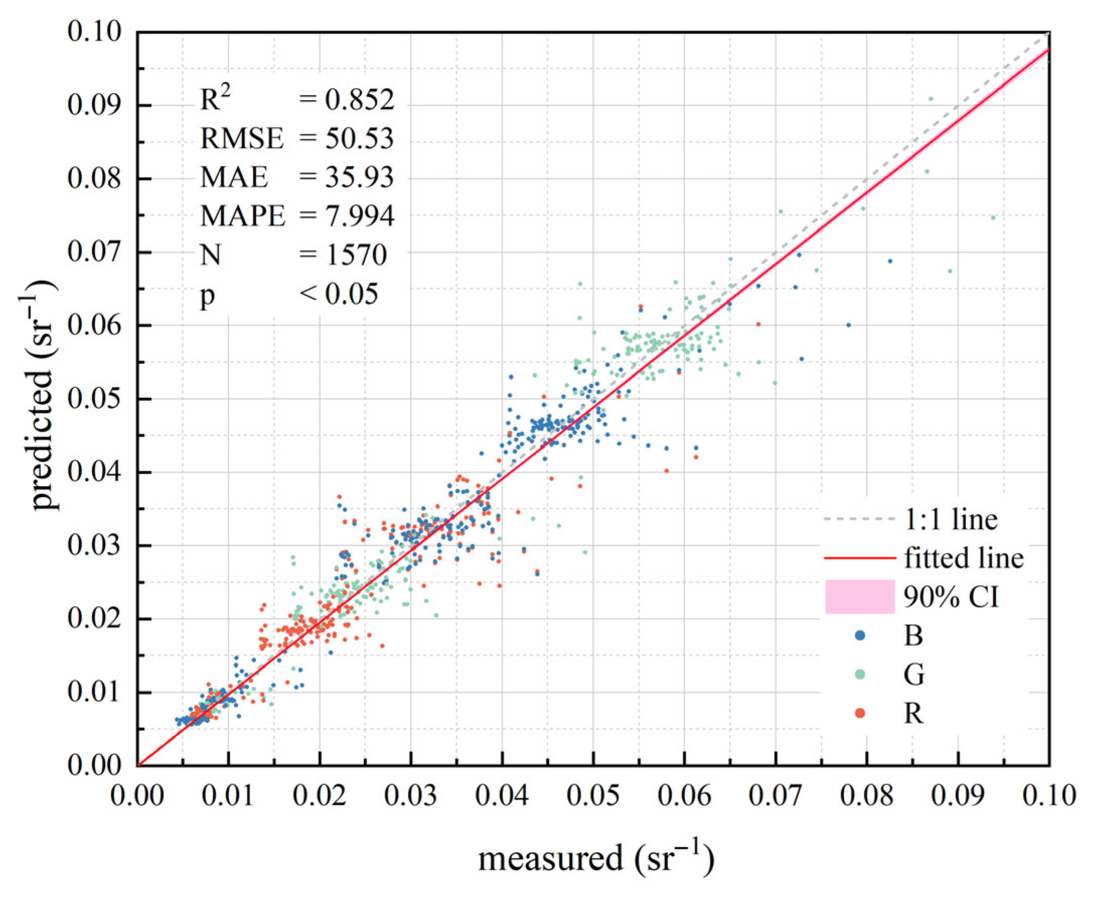
For the data in Section 2.3.2, the three visible light channels (B2, B3, and B4) were retained, and other conditions were kept unchanged. The results of the ETMNet neural network model training are presented in Figure 15.
As can be seen from Figure 15, when the UAV is equipped with only RGB (three) channels, the Transformer model optimized by ETO can still effectively fit the atmospheric effects in the satellite-to-ground radiative transfer process (with an overall fitting accuracy of R2 > 0.85), thereby achieving ASAC. Compared to hyperspectral sensors, RGB sensors have lower spectral resolution, and both the quantity and quality of surface-based AC reference data are reduced, resulting in a certain decline in GASAC accuracy. For RGB sensors with different band configurations and spectral response characteristics, the ASAC model exhibits a certain degree of generalizability, but the accuracy of atmospheric correction results may vary.

4.3. Discussion on GASAC

This section first validates, through comparative experiments, the advantages of the ETMNet-based GASAC model proposed in this study over other deep learning-based atmospheric correction baseline models and provides a theoretical analysis. Subsequently, the temporal generalization capability of the GASAC model is discussed, highlighting the necessity of synchronized data. The spatial distribution of Chl-a concentrations in the study area across different experimental periods is also mapped and analyzed.

4.3.1. Comparison Between GASAC and Baseline AC Models

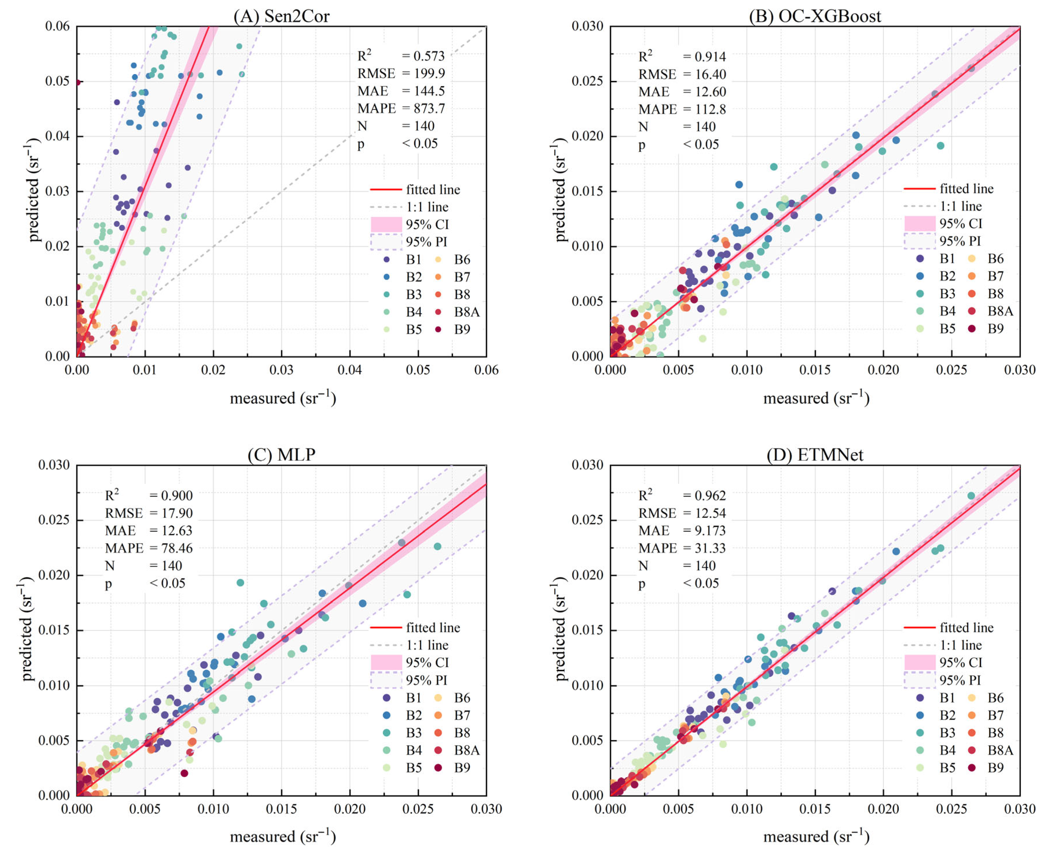
This study designed three control groups to validate the superiority of the proposed GASAC model. Group A utilizes Sentinel-2 Level-2A data, which incorporates atmospheric parameters measured by onboard sensors and applies the Sen2Cor deep learning atmospheric correction model—a widely adopted representative of deep learning-based AC models. Group B adopts the OC-XGBRT algorithm proposed by Song et al. (2023), which combines XGBoost with radiative transfer simulations and represents a state-of-the-art deep learning-based AC approach [19]. Group C employs an MLP architecture identical to the MLP component within ETMNet, used to assess the performance improvement brought by the Transformer architecture. Group D uses the ETMNet model developed in this study. All groups (A–D) utilize the same dataset described in Section 2.4.2. Groups B through D are trained using the ETO optimizer for 100 iterations, with all other settings kept consistent. The comparison results with ASD data are shown in Figure 16.
As shown in Figure 16, the GASAC method developed in this study outperforms both the commonly used Sen2Cor and the state-of-the-art deep learning model OC-XGBoost. In comparison with in situ ASD-derived water leave-off radiation, the correction accuracy (R2) increased by 0.389 and 0.048, respectively. Notably, compared to the latest baseline model, the Mean Absolute Percentage Error (MAPE) decreased by nearly 70%, demonstrating a significant advantage in atmospheric correction accuracy. Furthermore, when compared with the MLP model, the Transformer-based ETMNet showed a clear performance gain, with the correction R 2 increasing by 0.062 and M A P E reduced by 47.13 percentage points. This verifies the potential of the Transformer architecture in AC tasks and further highlights the superiority of the GASAC framework proposed in this study.
Sen2Cor estimates atmospheric parameters based on infrared, water vapor, ultraviolet, and other bands captured by satellite sensors. However, due to limited input parameters and globally distributed correction data, the model struggles to accurately fit the atmospheric characteristics of nearshore waters. OC-XGBoost, developed based on a large volume of in situ measurements from coastal environments, exhibits strong adaptability and achieves good atmospheric correction performance, but it remains constrained by assumptions in the radiative transfer model. In our comparison, ETMNet significantly outperformed OC-XGBoost, especially reducing MAPE by 72% [57]. This is vital for coastal water monitoring where small errors in low-radiance signals can lead to large relative errors, impacting the accuracy of chlorophyll-a retrieval. While MLP demonstrates strong nonlinear fitting capabilities, its lack of a self-attention mechanism limits its accuracy in small-sample regression tasks compared to Transformer-based models. The ETMNet proposed in this study integrates the fitting strength of MLP with enhanced small-sample adaptability through a multi-head self-attention mechanism and ETO optimization. As a result, it achieves superior AC accuracy and serves as the core of the proposed GASAC framework for nearshore environments.

4.3.2. Verifying Temporal Generalization Performance of the GASAC Model in This Study

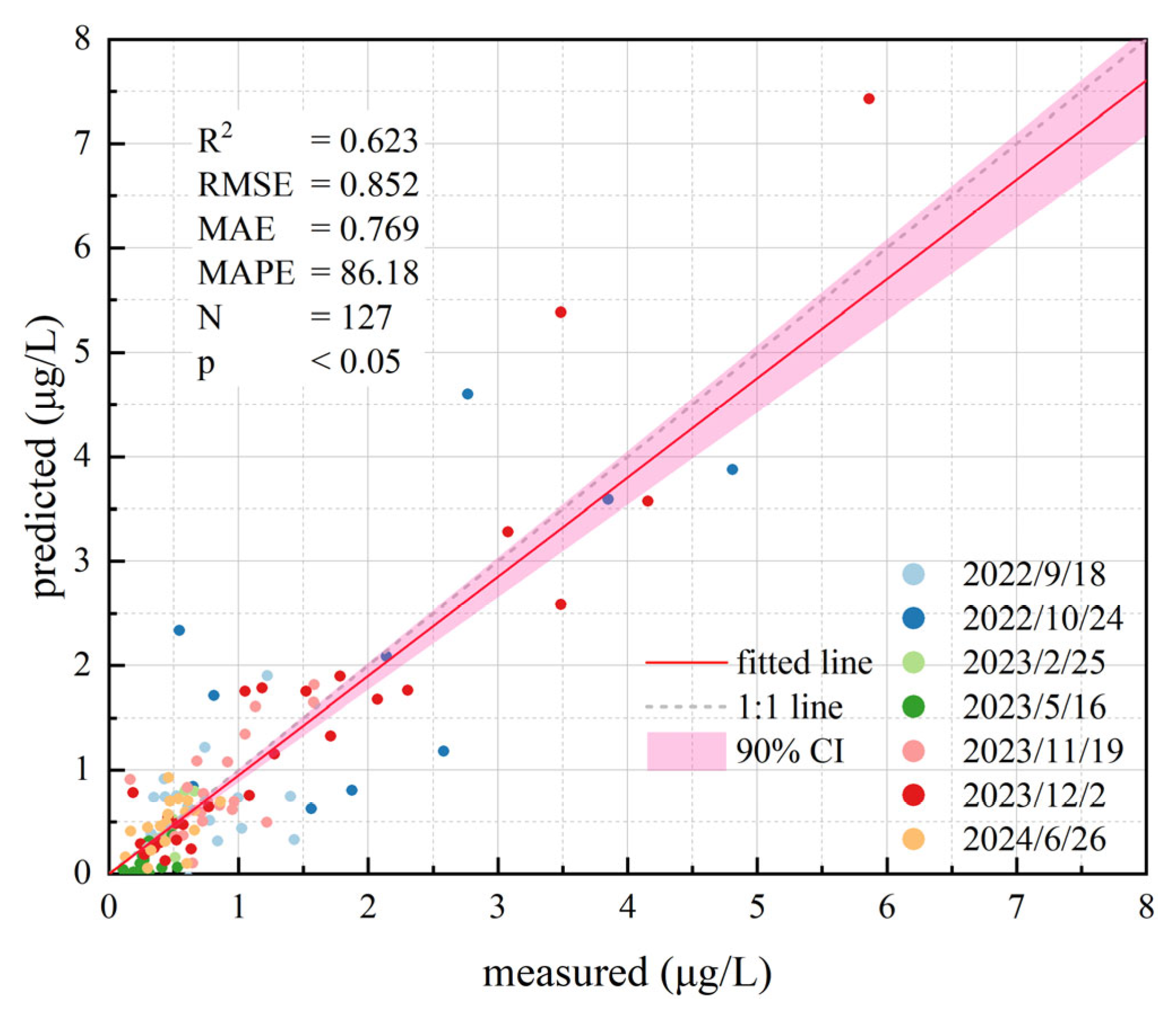
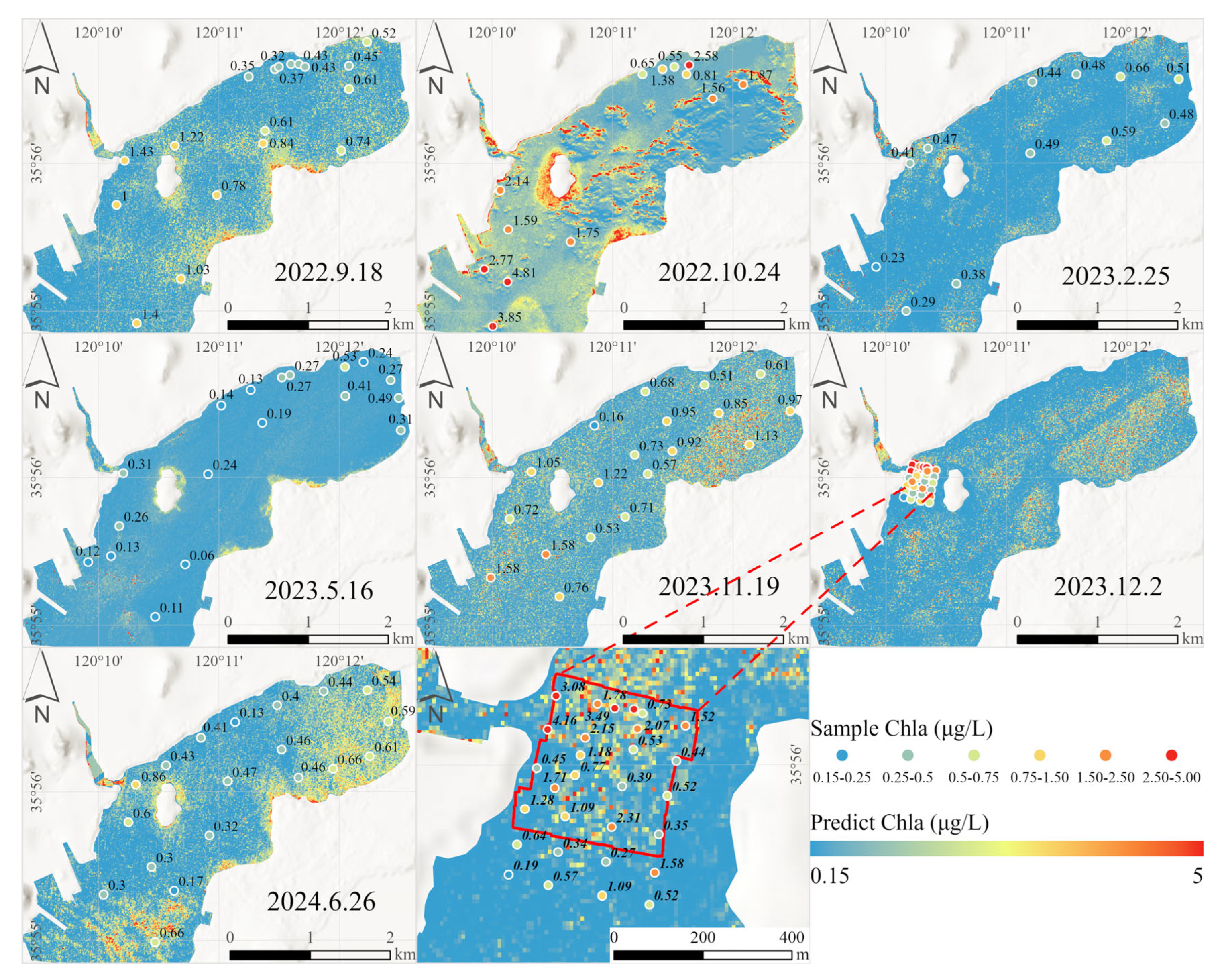
In order to investigate the applicability of the GASAC model to satellite images in other time periods, the resulting images obtained after GASAC of the remote sensing images of the study area during seven experimental periods were processed using Chl-a concentration inversion model, thereby obtaining the spatial distribution of Chl-a concentration in the study area. The predicted and measured scatter of Chl-a concentrations is shown in Figure 17. The points and values in Figure 18 represent the measuring points and the Chl-a concentration values measured at these points, and the colors represent the predicted values obtained after the application of the optimal Chl-a concentration inversion model to the post-GASAC S2 data. All of the seven experiments were conducted under clear-sky and cloudless conditions, and sampling was carried out during noon hours under conditions of good visibility, sufficient illumination, and similar atmospheric environments.
In general, the values of Chl-a concentration in the study area are mainly distributed within the range of 0.15–5 μ g / L and are mostly smaller than 0.5 μ g / L , indicating that the water body in the study area is clean. In terms of spatial distribution, the Chl-a concentration in the northwestern area of the estuary is significantly higher than than that in the surrounding areas, indicating that the release of pollutants produced by human activities has caused damage to the aquatic ecosystem in this area; the Chl-a concentration in the southeastern area of the estuary is higher than that in the surrounding areas, possibly due to the high concentration of pollutants caused by relatively low seawater mobility in this area; the Chl-a concentration along the central axis of the bay is relatively low because the drainage channel along this central axis was dredged on 2 December 2023, resulting in enhanced tidal water flow from the open waters outside the bay. For most sampling points, the inversion results are highly consistent with the measured data, indicating that the “ground-aerial-satellite” multistage atmospheric correction method can enable the application of the Chl-a concentration inversion model to multi-period satellite remote sensing data and deliver good prediction results.
All synchronized data collections in this experiment were conducted at noon under clear skies, low wind speeds, cloud-free conditions, and good visibility. While the atmospheric conditions were generally similar, slight differences existed between acquisition times. These differences were reflected in the correction results: the GASAC model achieved the highest correction accuracy for the synchronized in situ data collected on 2 December 2023, with a Chl-a inversion accuracy of R 2 = 0 .818 in Group D of Section 3.4.2. However, for the in situ data from other periods discussed in Section 4.3, the inversion accuracy dropped to R 2 = 0 .623. This indicates that while the GASAC model has a certain correction capability for remote sensing imagery acquired under similar meteorological conditions, its accuracy declines over time. Therefore, it is necessary to collect synchronized ground–aerial–satellite multi-scale data to capture more detailed atmospheric effects during different periods.

5. Conclusions

This study explores a GASAC approach for nearshore waters by integrating synchronously collected in situ water spectra, UAV imagery, and satellite imagery. The proposed method demonstrates high accuracy and regional applicability, achieving promising inversion performance when applied to concentration retrieval models. The main conclusions of this study are as follows:
(1)
Synchronously collected “ground–aerial–satellite” data from nearshore waters provide a large number of “pixel-to-pixel” atmospheric correction samples, revealing finer spatial distribution characteristics of water optical properties. These data offer continuous, sufficient, and accurate AC samples, enabling models with strong fitting capability to effectively learn the nonlinear atmospheric effects in satellite-to-aerial radiative transfer, thus exhibiting great potential for multi-scale cooperative atmospheric correction in nearshore environments.
(2)
The Transformer architecture, using an MLP as its base learner, shows strong capability in modeling nonlinear atmospheric effects. However, the volume of synchronized UAV–satellite AC samples with consistent spatial and spectral characteristics remains insufficient for deep learning. By incorporating the ETO strategy to guide parameter design and optimization of the Transformer, a robust, small-sample-adaptable, and high-performing model—ETMNet—can be constructed, achieving high-accuracy atmospheric correction in nearshore waters.
(3)
The experimental results show that, compared to the “point-to-pixel” GSAC method using only in situ spectra, the stepwise GASAC framework integrating all three data sources improves the R 2 of the predicted in situ water-leaving radiation from 0.837 to 0.962 and raises the Chl-a concentration inversion accuracy from 0.645 to 0.818. Compared to the latest baseline model, the R 2 of predicted in situ water-leaving radiation increased from 0.914 to 0.962.
In summary, the multi-scale, stepwise “ground–aerial–satellite” atmospheric correction model developed in this study can effectively eliminate atmospheric disturbances in satellite observations over nearshore waters. It reveals the application potential of synchronized “ground–aerial–satellite” data in satellite image atmospheric correction and is expected to be extended to more general RGB three-band UAV sensors, demonstrating promising application potential and practical significance for atmospheric correction in nearshore waters. This approach also provides a feasible strategy for high-precision water quality monitoring in coastal regions.
Despite the advantages of the proposed GASAC model for nearshore waters, the limited amount of in situ water-leaving radiation data—due to the challenges of collecting synchronized “ground–aerial–satellite” data—prevented a comprehensive validation of the model’s applicability across the entire study area. In future work, we will test the applicability of GASAC using UAV data equipped with RGB sensors to significantly enhance the operational feasibility of GASAC in nearshore water environments.

Author Contributions

Conceptualization, X.S. and J.C.; Methodology, X.S. and J.C.; Software, X.S. and W.G.; Validation, X.S.; Formal analysis, X.S.; Investigation, X.S., J.Z. and M.X.; Resources, J.Z.; Data curation, X.S.; Writing—original draft, X.S.; Writing—review & editing, X.S. and J.C.; Visualization, X.S.; Supervision, X.S., J.C., J.Z. and J.G.; Project administration, J.C., J.Z. and J.G.; Funding acquisition, J.Z. and J.G. All authors have read and agreed to the published version of the manuscript.

Funding

This work was supported in part by the National Natural Science Foundation of China under Grant U2106211.

Data Availability Statement

The Sentinel-2 satellite data used in this study can be accessed via the following link: https://browser.dataspace.copernicus.eu, accessed on 5 September 2024. The hyperspectral UAV imagery, Analytical Spectral Device (ASD) measured data, and chlorophyll-a (Chl-a) measured data can be provided upon request to the corresponding author.

Conflicts of Interest

The authors declare no conflict of interest.

References

  1. Pan, Y.; Shen, F.; Verhoef, W. An improved spectral optimization algorithm for atmospheric correction over turbid coastal waters: A case study from the Changjiang (Yangtze) estuary and the adjacent coast. Remote Sens. Environ. 2017, 191, 197–214. [Google Scholar] [CrossRef]
  2. Adjovu, G.E.; Stephen, H.; James, D.; Ahmad, S. Overview of the application of remote sensing in effective monitoring of water quality parameters. Remote Sens. 2023, 15, 1938. [Google Scholar] [CrossRef]
  3. McClain, C.R. A decade of satellite ocean color observations. Annu. Rev. Mar. Sci. 2009, 1, 19–42. [Google Scholar] [CrossRef]
  4. Shi, J.; Shen, Q.; Yao, Y.; Zhang, F.; Li, J.; Wang, L. Field Radiometric Calibration of a Micro-Spectrometer Based on Remote Sensing of Plateau Inland Water Colors. Appl. Sci. 2023, 13, 2117. [Google Scholar] [CrossRef]
  5. Zhang, Z.; Chen, P.; Zhang, S.; Huang, H.; Pan, Y.; Pan, D. A Review of Machine Learning Applications in Ocean Color Remote Sensing. Remote Sens. 2025, 17, 1776. [Google Scholar] [CrossRef]
  6. Ying, H.; Xia, K.; Huang, X.; Feng, H.; Yang, Y.; Du, X.; Huang, L. Evaluation of water quality based on UAV images and the IMP-MPP algorithm. Ecol. Inform. 2021, 61, 101239. [Google Scholar] [CrossRef]
  7. Frouin, R.; Pelletier, B. Fields of non-linear regression models for atmospheric correction of satellite ocean-color imagery. Remote Sens. Environ. 2007, 111, 450–465. [Google Scholar] [CrossRef]
  8. Jia, J.; Chen, C.; Liu, Q.; Ding, B.; Ren, Z.; Jia, Y.; Bai, X.; Du, R.; Chen, Q.; Wang, S. Soil salinity monitoring model based on the synergistic construction of ground-UAV-satellite data. Soil Use Manag. 2024, 40, e12980. [Google Scholar] [CrossRef]
  9. Zhu, X.; Chen, X.; Ma, L.; Liu, W. UAV and Satellite Synergies for Mapping Grassland Aboveground Biomass in Hulunbuir Meadow Steppe. Plants 2024, 13, 1006. [Google Scholar] [CrossRef] [PubMed]
  10. Lantzanakis, G.; Mitraka, Z.; Chrysoulakis, N. Comparison of physically and image based atmospheric correction methods for Sentinel-2 satellite imagery. In Perspectives on Atmospheric Sciences; Springer: Cham, Switzerland, 2017; pp. 255–261. [Google Scholar]
  11. Lee, K.H.; Yum, J.M. A review on atmospheric correction technique using satellite remote sensing. Korean J. Remote Sens. 2019, 35, 1011–1030. [Google Scholar] [CrossRef]
  12. Siegel, D.A.; Wang, M.; Maritorena, S.; Robinson, W. Atmospheric correction of satellite ocean color imagery: The black pixel assumption. Appl. Opt. 2000, 39, 3582–3591. [Google Scholar] [CrossRef]
  13. Mandanici, E.; Franci, F.; Bitelli, G.; Agapiou, A.; Alexakis, D.; Hadjimitsis, D.G. Comparison between empirical and physically based models of atmospheric correction. In Proceedings of the Third International Conference on Remote Sensing and Geoinformation of the Environment (RSCy2015), Paphos, Cyprus, 16–19 March 2015; pp. 110–119. [Google Scholar]
  14. Wei, J.; Yu, X.; Lee, Z.; Wang, M.; Jiang, L. Improving low-quality satellite remote sensing reflectance at blue bands over coastal and inland waters. Remote Sens. Environ. 2020, 250, 112029. [Google Scholar] [CrossRef]
  15. Mobley, C.D. Estimation of the remote-sensing reflectance from above-surface measurements. Appl. Opt. 1999, 38, 7442–7455. [Google Scholar] [CrossRef]
  16. Wang, C.; Myint, S.W. A simplified empirical line method of radiometric calibration for small unmanned aircraft systems-based remote sensing. IEEE J. Sel. Top. Appl. Earth Obs. Remote Sens. 2015, 8, 1876–1885. [Google Scholar] [CrossRef]
  17. Shah, M.; Raval, M.S.; Divakaran, S. A deep learning perspective to atmospheric correction of satellite images. In Proceedings of the IGARSS 2022–2022 IEEE International Geoscience and Remote Sensing Symposium, Kuala Lumpur, Malaysia, 17–22 July 2022; pp. 346–349. [Google Scholar]
  18. Acito, N.; Diani, M.; Corsini, G. CWV-Net: A deep neural network for atmospheric column water vapor retrieval from hyperspectral VNIR data. IEEE Trans. Geosci. Remote Sens. 2020, 58, 8163–8175. [Google Scholar] [CrossRef]
  19. Song, Z.; He, X.; Bai, Y.; Dong, X.; Wang, D.; Li, T.; Zhu, Q.; Gong, F. Atmospheric correction of absorbing aerosols for satellite ocean color remote sensing over coastal waters. Remote Sens. Environ. 2023, 290, 113552. [Google Scholar] [CrossRef]
  20. Duffy, K.; Vandal, T.J.; Wang, W.; Nemani, R.R.; Ganguly, A.R. A framework for deep learning emulation of numerical models with a case study in satellite remote sensing. IEEE Trans. Neural Netw. Learn. Syst. 2022, 34, 3345–3356. [Google Scholar] [CrossRef] [PubMed]
  21. Wang, Y.; Ti, R.; Liu, Z.; Liu, X.; Yu, H.; Wei, Y.; Fan, Y.; Wang, Y.; Huang, H.; Sun, X. Enhancing aerosol vertical distribution retrieval with combined LSTM and Transformer model from OCO2 O2 A-band observations. IEEE J. Sel. Top. Appl. Earth Obs. Remote Sens. 2025, 18, 9650–9665. [Google Scholar] [CrossRef]
  22. Cao, H.; Leng, H.; Zhao, J.; Xu, X.; Yang, J.; Li, B.; Zhou, Y.; Huang, L. Exploration of Deep-Learning-Based Error-Correction Methods for Meteorological Remote-Sensing Data: A Case Study of Atmospheric Motion Vectors. Remote Sens. 2024, 16, 3522. [Google Scholar] [CrossRef]
  23. Su, T.C. A study of a matching pixel by pixel (MPP) algorithm to establish an empirical model of water quality mapping, as based on unmanned aerial vehicle (UAV) images. Int. J. Appl. Earth Obs. Geoinf. 2017, 58, 213–224. [Google Scholar] [CrossRef]
  24. Román, A.; Tovar-Sánchez, A.; Gauci, A.; Deidun, A.; Caballero, I.; Colica, E.; D’Amico, S.; Navarro, G. Water-quality monitoring with a UAV-mounted multispectral camera in coastal waters. Remote Sens. 2022, 15, 237. [Google Scholar] [CrossRef]
  25. Inglada, J.; Muron, V.; Pichard, D.; Feuvrier, T. Analysis of artifacts in subpixel remote sensing image registration. IEEE Trans. Geosci. Remote Sens. 2006, 45, 254–264. [Google Scholar] [CrossRef]
  26. Dombi, J.; Dineva, A. Adaptive Savitzky-Golay filtering and its applications. Int. J. Adv. Intell. Paradig. 2020, 16, 145–156. [Google Scholar] [CrossRef]
  27. Lee, J.S. Refined filtering of image noise using local statistics. Comput. Graph. Image Process. 1981, 15, 380–389. [Google Scholar] [CrossRef]
  28. Ali, M.I.; Dirawan, G.D.; Hasim, A.H.; Abidin, M.R. Detection of changes in surface water bodies urban area with NDWI and MNDWI methods. Int. J. Adv. Sci. Eng. Inf. Technol. 2019, 9, 946–951. [Google Scholar] [CrossRef]
  29. Pitarch, J.; Vanhellemont, Q. The QAA-RGB: A universal three-band absorption and backscattering retrieval algorithm for high resolution satellite sensors. Development and implementation in ACOLITE. Remote Sens. Environ. 2021, 265, 112667. [Google Scholar] [CrossRef]
  30. Qun’ou, J.; Lidan, X.; Siyang, S.; Meilin, W.; Huijie, X. Retrieval model for total nitrogen concentration based on UAV hyper spectral remote sensing data and machine learning algorithms–A case study in the Miyun Reservoir, China. Ecol. Indic. 2021, 124, 107356. [Google Scholar] [CrossRef]
  31. Cheng, K.H.; Chan, S.N.; Lee, J.H.W. Remote sensing of coastal algal blooms using unmanned aerial vehicles (UAVs). Mar. Pollut. Bull. 2020, 152, 110889. [Google Scholar] [CrossRef]
  32. Gordon, H.R. Atmospheric correction of ocean color imagery in the Earth Observing System era. J. Geophys. Res. Atmos. 1997, 102, 17081–17106. [Google Scholar] [CrossRef]
  33. Kedzierski, M.; Wierzbicki, D.; Sekrecka, A.; Fryskowska, A.; Walczykowski, P.; Siewert, J. Influence of lower atmosphere on the radiometric quality of unmanned aerial vehicle imagery. Remote Sens. 2019, 11, 1214. [Google Scholar] [CrossRef]
  34. Acharya, B.S.; Bhandari, M.; Bandini, F.; Pizarro, A.; Perks, M.; Joshi, D.R.; Wang, S.; Dogwiler, T.; Ray, R.L.; Kharel, G. Unmanned aerial vehicles in hydrology and water management: Applications, challenges, and perspectives. Water Resour. Res. 2021, 57, e2021WR029925. [Google Scholar] [CrossRef]
  35. Holland, P.W.; Welsch, R.E. Robust regression using iteratively reweighted least-squares. Commun. Stat.-Theory Methods 1977, 6, 813–827. [Google Scholar] [CrossRef]
  36. Huang, J.C.; Ko, K.M.; Shu, M.H.; Hsu, B.M. Application and comparison of several machine learning algorithms and their integration models in regression problems. Neural Comput. Appl. 2020, 32, 5461–5469. [Google Scholar] [CrossRef]
  37. Gross, L.; Thiria, S.; Frouin, R. Applying artificial neural network methodology to ocean color remote sensing. Ecol. Model. 1999, 120, 237–246. [Google Scholar] [CrossRef]
  38. Yu, G.; Zhong, Y.; Fu, D.; Chen, F.; Chen, C. Remote sensing estimation of δ15NPN in the Zhanjiang Bay using Sentinel-3 OLCI data based on machine learning algorithm. Front. Mar. Sci. 2024, 11, 1366987. [Google Scholar] [CrossRef]
  39. Luan, T.M.; Khatir, S.; Tran, M.T.; De Baets, B.; Cuong-Le, T. Exponential-trigonometric optimization algorithm for solving complicated engineering problems. Comput. Methods Appl. Mech. Eng. 2024, 432, 117411. [Google Scholar] [CrossRef]
  40. Møller, M.F. A scaled conjugate gradient algorithm for fast supervised learning. Neural Netw. 1993, 6, 525–533. [Google Scholar] [CrossRef]
  41. Prechelt, L. Early stopping-but when? In Neural Networks: Tricks of the Trade; Springer: Berlin/Heidelberg, Germany, 2002; pp. 55–69. [Google Scholar]
  42. Srivastava, N.; Hinton, G.; Krizhevsky, A.; Sutskever, I.; Salakhutdinov, R. Dropout: A simple way to prevent neural networks from overfitting. J. Mach. Learn. Res. 2014, 15, 1929–1958. [Google Scholar]
  43. Yang, H.; Kong, J.; Hu, H.; Du, Y.; Gao, M.; Chen, F. A review of remote sensing for water quality retrieval: Progress and challenges. Remote Sens. 2022, 14, 1770. [Google Scholar] [CrossRef]
  44. Luo, J.; Qin, L.; Mao, P.; Xiong, Y.; Zhao, W.; Gao, H.; Qiu, G. Research progress in the retrieval algorithms for chlorophyll-a, a key element of water quality monitoring by remote sensing. Remote Sens. Technol. Appl. 2021, 36, 473–488. [Google Scholar]
  45. Cleveland, J.S. Regional models for phytoplankton absorption as a function of chlorophyll a concentration. J. Geophys. Res. Ocean. 1995, 100, 13333–13344. [Google Scholar] [CrossRef]
  46. Lohrenz, S.E.; Weidemann, A.D.; Tuel, M. Phytoplankton spectral absorption as influenced by community size structure and pigment composition. J. Plankton Res. 2003, 25, 35–61. [Google Scholar] [CrossRef]
  47. Niu, C.; Tan, K.; Wang, X.; Du, P.; Pan, C. A semi-analytical approach for estimating inland water inherent optical properties and chlorophyll a using airborne hyperspectral imagery. Int. J. Appl. Earth Obs. Geoinf. 2024, 128, 103774. [Google Scholar] [CrossRef]
  48. Cui, M. Introduction to the k-means clustering algorithm based on the elbow method. J. Account. Audit. Financ. 2020, 1, 5–8. [Google Scholar]
  49. Yu, X.; Liu, Q.; Liu, X.; Liu, X.; Wang, Y. A physical-based atmospheric correction algorithm of unmanned aerial vehicles images and its utility analysis. Int. J. Remote Sens. 2017, 38, 3101–3112. [Google Scholar] [CrossRef]
  50. Berk, A.; Anderson, G.P.; Bernstein, L.S.; Acharya, P.K.; Dothe, H.; Matthew, M.W.; Adler-Golden, S.M.; Chetwynd, J.H., Jr.; Richtsmeier, S.C.; Pukall, B. MODTRAN4 radiative transfer modeling for atmospheric correction. In Proceedings of the Optical Spectroscopic Techniques and Instrumentation for Atmospheric and Space Research III, Denver, CO, USA, 20 October 1999; pp. 348–353. [Google Scholar]
  51. Kennedy, J.; Eberhart, R. Particle swarm optimization. In Proceedings of the ICNN’95-International Conference on Neural Networks, Perth, WA, Australia, 27 November 1995; pp. 1942–1948. [Google Scholar]
  52. Forrest, S. Genetic algorithms. ACM Comput. Surv. (CSUR) 1996, 28, 77–80. [Google Scholar] [CrossRef]
  53. Glorot, X.; Bengio, Y. Understanding the difficulty of training deep feedforward neural networks. In Proceedings of the Thirteenth International Conference on Artificial Intelligence and Statistics, Sardinia, Italy, 13–15 May 2010; pp. 249–256. [Google Scholar]
  54. Hong, S.M.; Morgan, B.J.; Stocker, M.D.; Smith, J.E.; Kim, M.S.; Cho, K.H.; Pachepsky, Y.A. Using machine learning models to estimate Escherichia coli concentration in an irrigation pond from water quality and drone-based RGB imagery data. Water Res. 2024, 260, 121861. [Google Scholar] [CrossRef]
  55. Parra, L.; Ahmad, A.; Sendra, S.; Lloret, J.; Lorenz, P. Combination of machine learning and RGB sensors to quantify and classify water turbidity. Chemosensors 2024, 12, 34. [Google Scholar] [CrossRef]
  56. Shiraishi, H. New index for estimation of chlorophyll-a concentration in water with RGB value. Int. J. Eng. Technol. 2018, 18, 10–16. [Google Scholar]
  57. Zhou, Y.; Li, W.; Cao, X.; He, B.; Feng, Q.; Yang, F.; Liu, H.; Kutser, T.; Xu, M.; Xiao, F. Spatial-temporal distribution of labeled set bias remote sensing estimation: An implication for supervised machine learning in water quality monitoring. Int. J. Appl. Earth Obs. Geoinf. 2024, 131, 103959. [Google Scholar] [CrossRef]
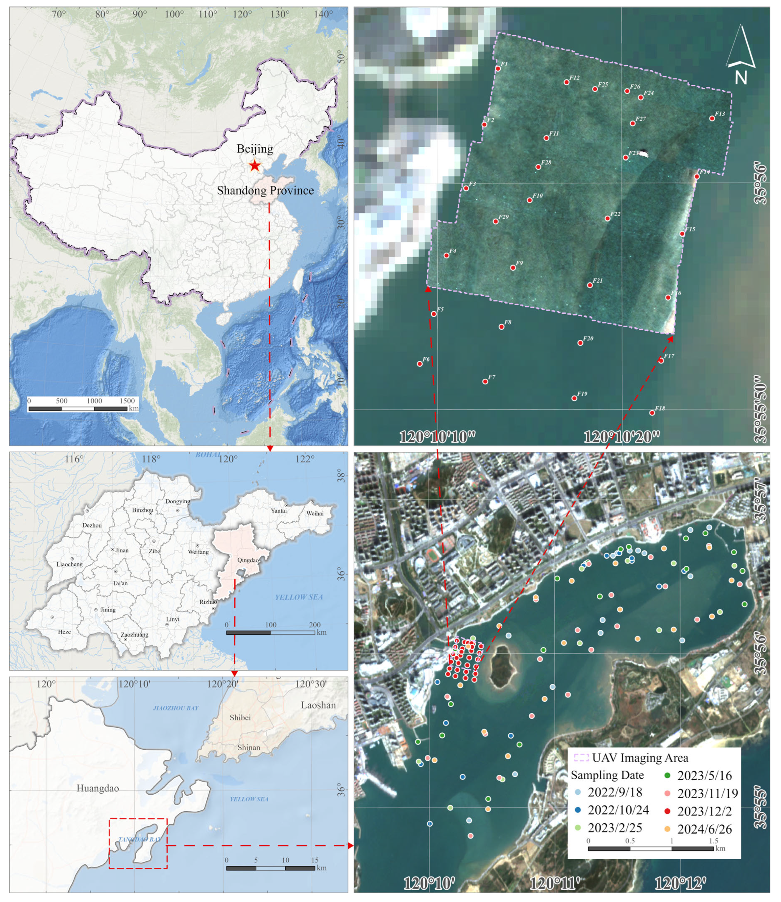
Figure 1. Study area and sampling point distribution.
Remotesensing 17 02768 g001
Figure 2. TriOS hyperspectral radiometer and spectral curves of measured water-leaving radiance data.
Remotesensing 17 02768 g002
Figure 3. Measured Chl-a concentration data (distribution).
Remotesensing 17 02768 g003
Figure 4. DJI M600 Pro hexacopter fitted with a Cubert S185 hyperspectral imager.
Remotesensing 17 02768 g004
Figure 5. Original and filtered UAV-HSI spectral curves.
Remotesensing 17 02768 g005
Figure 6. Equivalent Sentinel-2 reflectance spectra for three types of data.
Remotesensing 17 02768 g006
Figure 7. Main processes of GASAC and water quality testing.
Remotesensing 17 02768 g007
Figure 8. Flowchart of the GASAC method for coastal waters.
Remotesensing 17 02768 g008
Figure 9. Scatter plots for the GAAC test set using MPP-ELM and MODTRAN 5.
Remotesensing 17 02768 g009
Figure 10. Scatter plot of water-leaving radiance predicted by ETMNet.
Remotesensing 17 02768 g010
Figure 11. Evaluation of the results of Transformer training achieved by different optimizers.
Remotesensing 17 02768 g011
Figure 12. Four types of atmospheric correction results vs. actual ASD data.
Remotesensing 17 02768 g012
Figure 13. Scatter plot of the results produced by the optimal Chl-a concentration inversion model.
Remotesensing 17 02768 g013
Figure 14. Chl-a concentration prediction results from four atmospheric correction methods.
Remotesensing 17 02768 g014
Figure 15. Scatter plot of water-leaving radiance predicted by the ETMNet based on UAV-RGB data.
Remotesensing 17 02768 g015
Figure 16. Water leave-off radiation prediction accuracy between GASAC and baseline AC models.
Remotesensing 17 02768 g016
Figure 17. Measured vs. predicted Chl-a concentration values obtained after GASAC of S2 images on several experimental dates.
Remotesensing 17 02768 g017
Figure 18. Spatial distribution of Chl-a concentration predicted after GASAC of S2 images on several experimental dates.
Remotesensing 17 02768 g018
Table 1. Hyperspectral radiometer (ASD) performance parameters and data acquisition parameters.
Analytical Spectral DeviceAWRMMS
ManufacturerTriOS (Made in Germany)
Spectral Range320–946 nm
Spectral Resolution1 nm
Sampling Time10:00–13:00 (UTC+8)
Sampling Depth≈1 m
Angle between Telescopic Pole Orientation and Solar Incidence Plane135°
Table 2. Performance parameters of the Cubert S185 hyperspectral imager (non-exhaustive).
Spectral Range (nm)450–998EFL (mm)16
Spectral Resolution (nm)≤8FOV (degree)23
Sampling Interval (nm)4Imaging Speed (Cubes·s−1)5
Spectral Trunnel138Imaging Size (px)103 × 103
Table 3. Feature combinations for Chl-a concentration inversion.
TypeCombinatorial FormulaRepresentative FeaturesCorrelation Abs Value
Double Bands R λ 1 R λ 2 B1 − B50.67
R ( λ 1 ) / R ( λ 2 )   B2/B30.77
R λ 1 R λ 2 R λ 1 + R λ 2 (B2 − B3)/(B2 + B3)0.80
Trible Bands R λ 1 R λ 2 R λ 3 B2/(B2 − B3)0.56
R λ 1 1 / R ( λ 2 ) 1 / R ( λ 3 )   B3/(1/B2 − 1/B3)0.83
Quadruple Bands 1 R λ 1 1 R λ 2 × 1 R λ 3 1 R λ 4 ( 1 / B 1     1 / B 9 ) × (1/B5 − 1/B8A)0.63
Table 4. Chl-a concentration inversion model parameters.
TypeInputsRegression ModelFormula
C h l a = f x x = R r s combination features
x = IOPs features
linear C h l a = a x + b
quadratic C h l a = a x 2 + b x + c
exponential function C h l a = a e b x
idempotent function C h l a = a x b
C h l a = f x , y x = R r s combination features
y = IOPs features
linear C h l a = a x + b y + c
quadratic C h l a = a x 2 + b y 2 + c x + d y + e
exponential function C h l a = a e b x + c e d y
idempotent function C h l a = a x b + c y d
Disclaimer/Publisher’s Note: The statements, opinions and data contained in all publications are solely those of the individual author(s) and contributor(s) and not of MDPI and/or the editor(s). MDPI and/or the editor(s) disclaim responsibility for any injury to people or property resulting from any ideas, methods, instructions or products referred to in the content.