Sparse Decomposition-Based Anti-Spoofing Framework for GNSS Receiver: Spoofing Detection, Classification, and Position Recovery

Abstract

Achieving reliable navigation is critical for GNSS receivers subject to spoofing attacks. Utilizing the inherent sparsity and inconsistency of spoofing signals, this paper proposes an anti-spoofing framework for GNSS receivers to detect, classify, and recover positions from spoofing attacks without additional devices. A sparse decomposition algorithm with non-negative constraints limited by signal power magnitudes is proposed to achieve accurate spoofing detections while extracting key features of the received signals. In the classification stage, these features continuously refine each channel of the receiver’s code tracking loop, ensuring that it tracks either the authentic or counterfeit signal components. Moreover, by leveraging the inherent inconsistency of spoofing properties, we incorporate the Hausdorff distance to determine the most overlapped position sets, distinguishing genuine trajectories and mitigating spoofing effects. Experiments on the TEXBAT dataset show that the proposed algorithm detects 98% of spoofing attacks, ensuring stable position recovery with an average RMSE of 6.32 m across various time periods.

1. Introduction

Global Navigation Satellite Systems (GNSS) offer worldwide coverage along with precise, reliable, and real-time position, velocity, and timing (PVT) services [1]. At the same time, such systems are inherently vulnerable due to the fragility of the signals [2], which primarily stems from two factors: (i) the limited power of GNSS signals on the ground, and (ii) the open structure of these signals. Their resulting fragility makes GNSS signals susceptible to instances of satellite spoofing interference, including spoofing attacks on portable GNSS receivers, unmanned aerial vehicles, and ships [3,4]. Unfortunately, most commercial GNSS receivers are not equipped with effective countermeasures against such spoofing attacks [5].

The main challenge faced by most commercial GNSS receivers in handling spoofing interference is that when under attack, their tracking loops cannot resist external drag-off from spoofing signal, resulting in continuous generation of fake position results. This problem is further aggravated during hybrid jamming–spoofing attacks [6]. In such scenarios, the attacker first transmits high-power jamming signals to prevent the receiver from acquiring authentic satellites. When acquisition is blocked, the attacker switches to high-power spoofing transmissions, which the receiver may mistakenly lock onto during startup. These increasingly sophisticated spoofing strategies highlight the need for robust countermeasures capable of detecting spoofing interference and mitigating its impact on receiver position solutions.

Currently, the majority of anti-spoofing algorithms for GNSS receivers concentrate on spoofing detection [7,8,9]. Spoofing classification was accomplished by [10] through spoofing and authentic parameter estimation. However, merely detecting or classifying spoofing signals is not enough; the more challenging and crucial task lies in eliminating the impact of spoofing signals on receivers that have already been spoofed and ensuring the generation of authentic PVT results.

To address these issues, methods based on multiple antennas that involve controlling the antenna steering patterns have been proposed to generate nulls and eliminate spoofing signals [11,12]. Furthermore, sensor fusion-based anti-spoofing interference techniques were propose in [13,14]. Using a fifth-generation (5G) signal base station has also proven helpful in spoofing mitigation [15]. However, the above approaches rely on adding extra devices to increase information redundancy, which not only increases costs but also limits the application scenarios of anti-spoofing algorithms for GNSS receivers [16]. The design of an anti-spoofing framework that relies on the observed data of only a single GNSS receiver to achieve reliable position results in generic scenarios remains an open problem worthy of further investigation.

To avoid excessive utilization of extra devices, Receiver Autonomous Integrity Measurement (RAIM) [17] provides a statistical reliability testing method which assumes a scenario in which a single visible satellite is spoofed. While effective, RAIM cannot discern spoofing when most channels are subject to spoofing, which is often the case during spoofing attacks. Lately, algorithms proposed by in [18,19] have employed vector tracking loops to estimate the magnitude, propagation delay, and carrier phase of spoofing attacks. However, this approach relies on prior assumptions such as classifying signals with higher amplitudes and longer delays as inauthentic, which may not be valid in common matched-power and intermediate spoofing scenarios. To address this limitation, the design of a Maximum Likelihood Estimation (MLE) principle with multiple correlator arrays was presented in [20] to estimate and then mitigate GNSS spoofing attacks. In [5], the authors introduced transitioning between multipath estimation of the delay lock loop and coupled amplitude delay lock loop for continuously tracking of authentic signal components. Nevertheless, the methods proposed in [5,20] both assume that the receiver operates normally during tracking before spoofing begins. This assumption is often unrealistic, since in practice it is difficult for a receiver to determine exactly when a spoofing attack begins.

In addition, many of the above methods [5,17,18,19,20] focus on identifying and mitigating attacks based on self-defined prior knowledge or assumptions during the tracking stage. These spoof mitigation strategies cannot track all contributing components simultaneously to achieve both authentic and fake pseudo-range measurements for each satellite. As a result, they miss opportunities to exploit redundant information deep within during the navigation phase of position computation, making them more difficult to apply in more general scenarios that go beyond prior assumptions.

Motivated by the above discussion, we propose a novel anti-spoofing framework for solving the spoofing detection, classification, and position recovery problem of GNSS receivers under frequency-locked spoofing attacks. The salient feature of our algorithm is that it continuously tracks all the received signals’ contributing components and further exploits the intrinsic inconsistency of the spoofing signals, thereby eliminating the need for additional limitations such as added extra devices, prior assumptions, and specific initial states. Compared with the existing literature, the main contributions of this work are highlighted as follows:

(1)

Unlike methods the proposed in [7,8,9], which only focus on spoofing detection, we devise a sparse decomposition algorithm with non-negative constraints limited by received signal power magnitudes, which not only achieves accurate spoofing detection but also simultaneously extracts key features of the received signal’s contributing components, achieving reliable spoofing classification.

(2)

Distinct from the methods introduced in [5,17,18,19,20], we adopt Advanced Iterative Hard Thresholding (AIHT) to integrate the key features extracted from our sparse decomposition method into Auxiliary Peak Tracking (APT), enabling separate tracking of spoofing and authentic components of each satellite to derive the true and spoofed pseudo-range measurements of each satellite. In this way, the intrinsic inconsistency of the spoofing signals can be further exploited without any extra devices and prior assumptions.

(3)

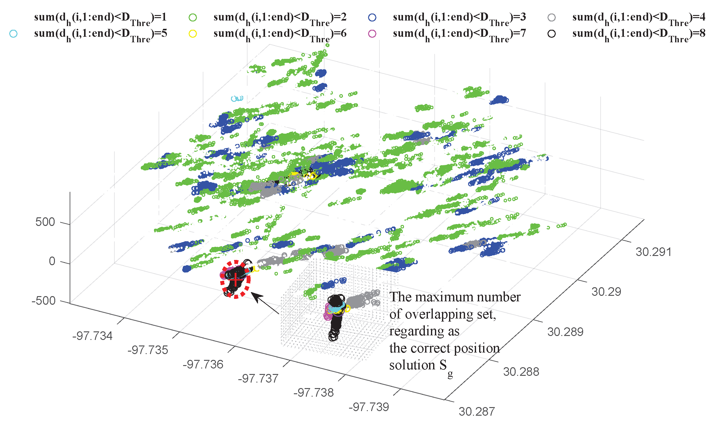
By leveraging the inherent inconsistency of spoofing properties, we incorporate the Hausdorff distance to determine the most overlapped position sets to identify genuine position trajectories in general scenarios. Compared with the methods proposed in [10,18,20], this mitigates the impacts of spoofing in position recovery without specific initial state limitations.

(4)

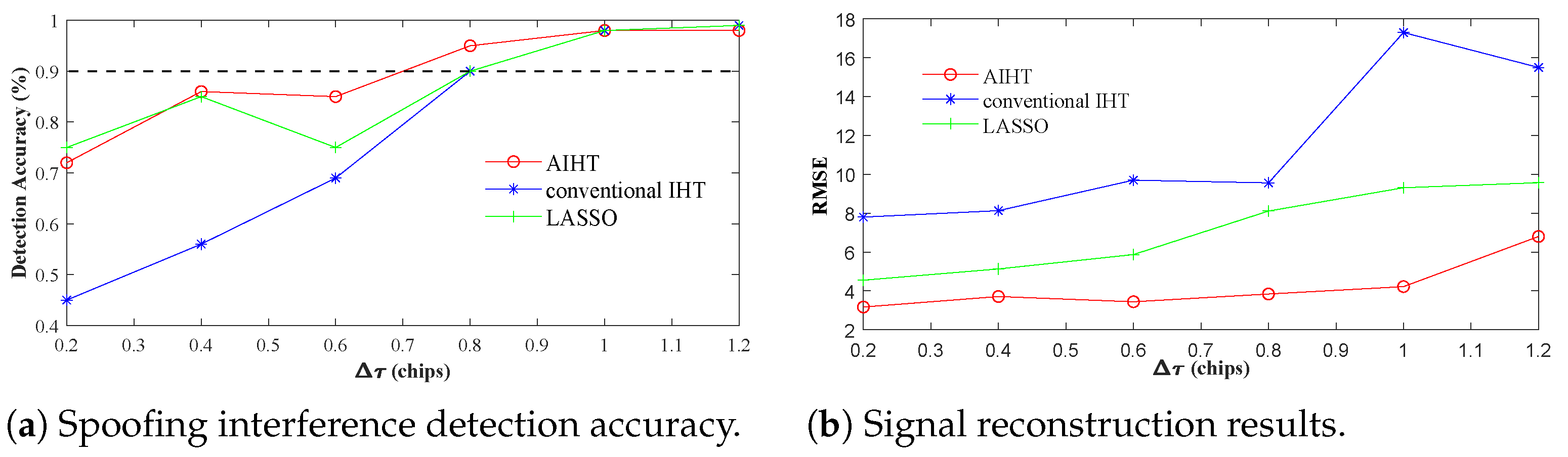
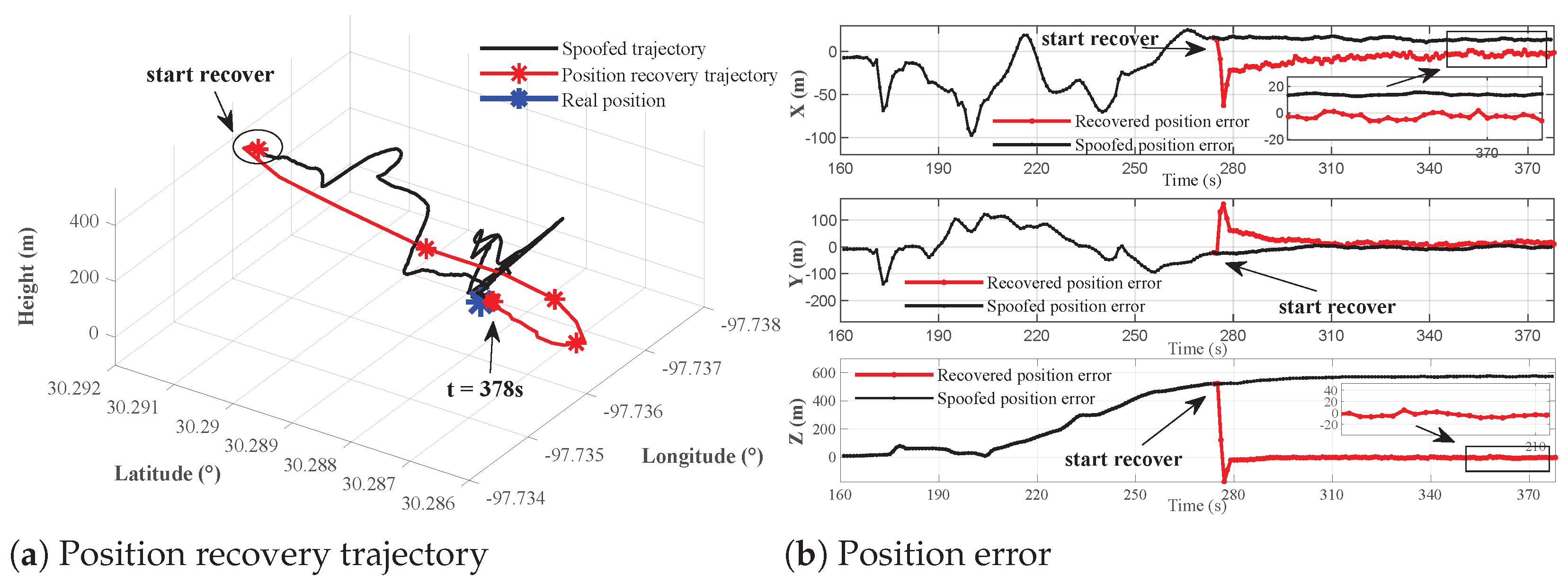
The efficacy and advantage of the proposed anti-spoofing framework are fully illustrated by extensive experiments conducted on the public TEXBAT dataset, showing that our algorithm detects 98% of spoofing attacks and guarantees stable position recovery with an average RMSE of 6.32 m across various time periods.

The rest of this paper is organized as follows: the spoofing signal model and analysis of the spoofed receiver correlators are provided in Section 2; Section 3 presents the design process of the sparse decomposition-based spoofing detection, classification, and position recovery framework; Section 4 shows the experimental results conducted with the TEXBAT dataset; Finally, Section 6 concludes the paper.

2. Problem Background

2.1. Spoofing Signal Model

After down-conversion from radio frequency (RF), the received signals in each channel of the receiver are composed of base-band GNSS signals and thermal noise. Without loss of generality, the GPS L1 signal is taken as the representative of different types of satellite signals in the following sections. The structure of a typical down-converted GPS L1 signal in the ith channel is described as follows:

$$\begin{array}{c}\hfill s_{\mathrm{ai}}\left(mT\right)=\sqrt{P_{\mathrm{ai}}}{C}_{\mathrm{i}}\left(mT-{\tau }_{\mathrm{ai}}\right)D_{\mathrm{i}}\left(mT\right)e^{j(2\pi f_{\mathrm{i}}mT+{\theta }_{\mathrm{ai}})}\end{array}$$

(1)

where the subscript label ${*}_a$ usually refers to parameters of an authentic satellite signal, ${*}_i$ refers to the parameters of the ith channel in the receiver, $P_{\mathrm{ai}}$ is the power of the received authentic signal, m is the discrete sample index of the tracking start time, T is the sampling period defined in a software receiver, ${\tau }_{\mathrm{ai}}$ and $f_{\mathrm{i}}$ respectively denote the code phase and Doppler frequency, ${\theta }_{\mathrm{ai}}$ is the carrier phase parameter, and $C_{\mathrm{i}}$ and $D_{\mathrm{i}}$ represent the C/A spreading code and the navigation message, respectively.

Similarly, the frequency-locked spoofing attack [10] of $s_{\mathrm{ai}}\left(mT\right)$, which is carried out by intermediate spoofers and replicate authentic Doppler frequency $f_{\mathrm{i}}$, is formulated as follows:

$$\begin{array}{ccc}\hfill & s_{\mathrm{si}}\left(mT\right)=\hfill & \hfill \sqrt{P_{\mathrm{si}}}{C}_{\mathrm{si}}\left(mT-{\tau }_{\mathrm{si}}\right)D_{\mathrm{i}}\left(mT\right)e^{j(2\pi f_{\mathrm{i}}mT+{\theta }_{\mathrm{si}})}\end{array}$$

(2)

where the subscript label ${*}_s$ means a counterfeit signal, while $P_{\mathrm{si}}$, ${\tau }_{\mathrm{si}}$ and ${\theta }_{\mathrm{si}}$ respectively represent the power, code, and carrier parameters of the spoofing signal $s_{\mathrm{si}}\left(mT\right)$ in the ith channel. According to Equations (1) and (2), when spoofing attack exists, the received signal $s_{\mathrm{i}}\left(mT\right)$ in the ith channel is modeled as

$$s_{\mathrm{i}}\left(mT\right)=s_{\mathrm{ai}}\left(mT\right)+s_{\mathrm{si}}\left(mT\right)+n\left(mT\right),$$

(3)

where $n\left(mT\right)$ is assumed to be Additive White Gaussian Noise (AWGN) combined with loop noise. To prevent the navigation message $D_{\mathrm{i}}\left(mT\right)$ from changing during two consecutive integration periods, the coherent integration period $T_0$ is maintained at less than half the bit duration. This ensures a constant navigation bit, and is omitted in the subsequent discussions in this article.

2.2. Analysis of the Spoofed Receiver Correlators

In the tracking process, the local replicas are generated by GNSS receivers to continuously achieve carrier and code wipe-off, and the locally constructed replica in the ith channel is provided as follows:

$$r\left(mT,\widehat{{\tau }_{\mathrm{i}}}\right)=C_{\mathrm{i}}\left(mT-\widehat{{\tau }_{\mathrm{i}}}\right)e^{j(2\pi f_{\mathrm{i}}mT+\widehat{{\theta }_{\mathrm{i}}})}$$

(4)

where ${\widehat{\tau }}_{\mathrm{i}}$ and ${\widehat{\theta }}_{\mathrm{i}}$ represent the estimated code and carrier parameters in time, respectively. By leveraging the local replica $r\left(mT,\widehat{{\tau }_{\mathrm{i}}}\right)$ in Equation (4), the correlator outcome in the ith channel $y\left({\tau }_{\mathrm{i}}\right)$ is

$$\begin{array}{cc}\hfill y\left({\tau }_{\mathrm{i}}\right)=& {\displaystyle \frac{1}{N_{\mathrm{c}}}}\sum _m^{m+N_{\mathrm{c}}-1}{s}_{\mathrm{i}}\left(mT\right)r{\left(mT,\widehat{{\tau }_{\mathrm{i}}}\right)}^{*}\hfill \\ \hfill =& \sqrt{P_{\mathrm{ai}}}R\left(\Delta {\tau }_{\mathrm{ai}}\right)e^{j\Delta {\theta }_{\mathrm{A}}}+\sqrt{P_{\mathrm{si}}}R\left(\Delta {\tau }_{\mathrm{si}}\right)e^{j\Delta {\theta }_{\mathrm{S}}}+\tilde{\mathit{\eta }}\hfill \\ \hfill =& y_{\mathrm{A}}\left({\tau }_{\mathrm{i}}\right)+y_{\mathrm{S}}\left({\tau }_{\mathrm{i}}\right)+\tilde{\eta }\hfill \end{array}$$

(5)

with

$$\begin{array}{c}\hfill \Delta {\tau }_{\mathrm{si}}={\tau }_{\mathrm{si}}-{\widehat{\tau }}_{\mathrm{i}},\Delta {\tau }_{\mathrm{ai}}={\tau }_{\mathrm{ai}}-{\widehat{\tau }}_{\mathrm{i}},\Delta {\theta }_{\mathrm{si}}={\theta }_{\mathrm{si}}-{\widehat{\theta }}_{\mathrm{i}},\Delta {\theta }_{\mathrm{ai}}={\theta }_{\mathrm{ai}}-{\widehat{\theta }}_{\mathrm{i}},\end{array}$$

where $N_{\mathrm{c}}=f_{\mathrm{s}}{T}_0$ is the number of samples of the coherent integration period $T_0$ and $f_{\mathrm{s}}={\displaystyle \frac{1}{T_0}}$ is the sampling frequency. In addition, ${\left(·\right)}^{*}$ denotes the complex conjugate operator, $R\left(·\right)$ denotes the auto-correlation function (ACF) depicted as an isosceles triangle, $\tilde{\mathit{\eta }}$ is the combination of different noise components, including the thermal noise in real signals and counterfeit signals, and $y_{\mathrm{A}}\left({\tau }_{\mathrm{i}}\right)$ and $y_{\mathrm{S}}\left({\tau }_{\mathrm{i}}\right)$ respectively denote the authentic signal correlation component and spoofing signal correlation component.

It is worth noting that ${\tau }_{\mathrm{i}}$ represents discrete time indexes, which is related to the estimated parameter $\widehat{{\tau }_{\mathrm{i}}}$. When ${\tau }_{\mathrm{i}}$ takes different values, a sequence $\mathit{R}\left(mT\right)$ of local replica elements with incremental time delays D is constructed, forming a post-correlation vector $\mathit{y}={\left[y\left({\tau }_{\mathrm{i}}+D\right)\dots y\left({\tau }_{\mathrm{i}}+ND\right)\right]}^T$. Here, N is the number of correlator taps, which can be rewritten as follows:

$$\begin{array}{c}\hfill \mathit{y}={\mathit{y}}_{\mathrm{A}}+{\mathit{y}}_{\mathrm{S}}+\tilde{\mathit{\eta }}\end{array}$$

(6)

where $\tilde{\mathit{\eta }}$ is the noise vector of $\tilde{\mathit{\eta }}$ in different taps, while ${\mathit{y}}_{\mathrm{A}}={\left[y_{\mathrm{A}}\left({\tau }_{\mathrm{i}}+D\right)\dots y_{\mathrm{A}}\left({\tau }_{\mathrm{i}}+ND\right)\right]}^T$ and ${\mathit{y}}_{\mathrm{S}}={\left[y_{\mathrm{S}}\left({\tau }_{\mathrm{i}}+D\right)\dots y_{\mathrm{S}}\left({\tau }_{\mathrm{i}}+ND\right)\right]}^T$ respectively represent the ACF envelops of the real and counterfeit signal components of $\mathit{y}$.

As shown in Equation (6), the postcorrelation vector $\mathit{y}$ is composed of two main components when the satellite signal is spoofed, namely, an authentic signal correlation component ${\mathit{y}}_{\mathrm{A}}$ and a spoofing signal correlation component ${\mathit{y}}_{\mathrm{S}}$. The same conclusion can also be drown in any correlator outcome elements $y\left({\tau }_{\mathrm{i}}\right)$:

$$\begin{array}{c}\hfill y\left({\tau }_{\mathrm{i}}\right)=y_{\mathrm{A}}\left({\tau }_{\mathrm{i}}\right)+y_{\mathrm{S}}\left({\tau }_{\mathrm{i}}\right)+\tilde{\eta }.\end{array}$$

(7)

Figure 1 shows how $y\left({\tau }_{\mathrm{i}}\right)$ is distorted by the spoofing component $y_{\mathrm{S}}\left({\tau }_{\mathrm{i}}\right)$, altering its normal triangular shape. This figure also details the drag-off process in delay-locked loops (DLLs) at various stages. As the code phase gap $\Delta {\tau }_{\mathrm{as}}={\tau }_{\mathrm{ai}}-{\tau }_{\mathrm{si}}$ between $y_{\mathrm{A}}\left({\tau }_{\mathrm{i}}\right)$ and $y_{\mathrm{S}}\left({\tau }_{\mathrm{i}}\right)$ widens, the DLLs are increasingly misled into locking onto $y_{\mathrm{S}}\left({\tau }_{\mathrm{i}}\right)$. When the drag-off process is complete, ${\mathit{y}}_{\mathrm{S}}$ gains control of the DLLs, indicating a successful spoofing attack. In this study we focus on frequency-locked attacks, which presents a more sophisticated challenge for detection and mitigation efforts than the unlocked attacks due to decoupling of the carrier phase changes from code phase shifts [21].

3. Methodology

To recover generic positions of the GNSS receivers under spoofing attacks, the following design procedure is provided and utilized, as shown in Figure 2:

i

In the detection phase, we leverage the sparse nature of the spoofed ACF and apply the AIHT algorithm with an additional non-negative constraint to enhance the accuracy of spoofing interference detection;

ii

During the classification stage, we introduce an AIHT-based APT method that tracks both authentic and counterfeit components of the same satellite using dual channels, termed a channel pair. Using code phase gap estimations from the modified AIHT, this method allows for continuous adjustments to the channel pairs.

iii

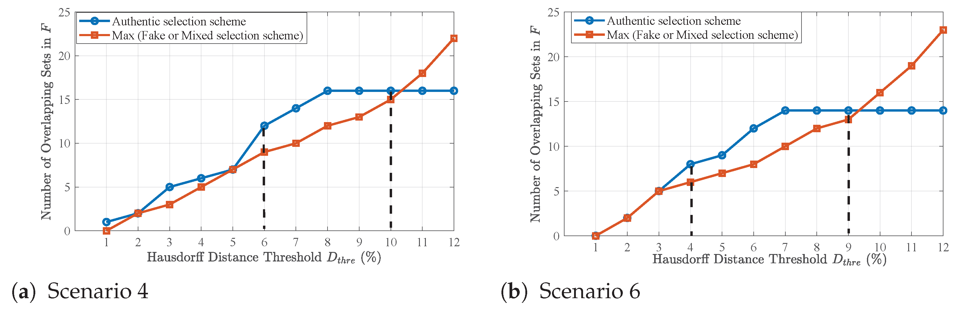
Finally, by employing different selection schemes, we obtain various position results; we then apply Hausdorff distance to identify the most consistent result, where the greatest number of candidate position sets overlap. This result is considered to be the true position, and the channels within the corresponding selection scheme are recognized for tracking authentic components.

3.1. Sparse Decomposition-Based Spoofing Detection

According to findings in [22], the spoofed postcorrelation vector outcome $\mathit{y}$ inherently possesses a sparse representation in the original domain, which is provided as follows:

$$\begin{array}{c}\hfill \underset{\mathit{y}}{\underbrace{\left[\begin{array}{c}y\left({\tau }_1\right)\\ ⋮\\ y\left({\tau }_{\mathrm{n}}\right)\end{array}\right]}}=\underset{\mathit{Q}}{\underbrace{\left[\begin{array}{ccc}{q}_{11}& \dots & q_{1\mathrm{n}}\\ ⋮& \ddots & ⋮\\ q_{\mathrm{n}1}& \dots & q_{\mathrm{n}\mathrm{n}}\end{array}\right]}}\underset{\mathit{\beta }}{\underbrace{\left[\begin{array}{c}{\mathit{\beta }}_1\\ ⋮\\ {\mathit{\beta }}_{\mathrm{n}}\end{array}\right]}}+\mathit{e}\end{array}$$

(8)

where $\mathit{Q}$ is a high-resolution dictionary, $\mathit{\beta }$ is a sparse vector, and $\mathit{e}\sim \mathcal{N}(0,{\sigma }^2\mathbf{I})$ represents the observation error due to loop noise and hardware limitations, with variance ${\sigma }^2$.

The underlying assumption of this sparse representation of $\mathit{y}$ is that $\mathit{y}$ exhibits sparsity in the ACF dictionary domain, particularly under spoofing attacks. In the context of compressed sensing, a vector $x\in {\mathbb{R}}^n$ is considered sparse if only a small number of its components are significantly nonzero, i.e., ${\parallel x\parallel }_0\ll n$, where ${\parallel x\parallel }_0$ denotes the number of nonzero elements. Under spoofing conditions, the ACF profile exhibits two dominant correlation peaks, one from the authentic signal and one from the spoofed signal; all other components are negligible, and primarily arise from thermal noise or weak multipath effects. This results in the sparse representation in (8), where the associated sparse coefficient vector $\mathit{\beta }$ has only a few nonzero elements corresponding to those dominant code phases, satisfying ${\parallel \mathit{\beta }\parallel }_0\ll n$.

As introduced by [10], the high-resolution dictionary $\mathit{Q}$ depicted in Figure 3 is composed of N m-sequence ACF triangle vectors with different code delays, which is modeled as follows:

$$\begin{array}{c}\hfill \mathit{Q}={\left[\mathit{R}{\left(0)\right)}^T\dots \mathit{R}{\left((N-1)D)\right)}^T\right]}^T\end{array}$$

(9)

where $\mathit{R}\left({\tau }_{\mathrm{i}}\right)=\left[R\left({\tau }_{\mathrm{i}}\right)\dots R({\tau }_{\mathrm{i}}-(N-1)D)\right]$ is the ACF triangle vector of m-sequence at code phase ${\tau }_{\mathrm{i}}$.

Given $\mathit{y}$ aggregates ACF triangles of each signal component with distinct amplitude and code phases, and understanding the role of the dictionary $\mathit{Q}$, the operation $\mathit{Q}*\mathit{\beta }$ aims to reconstruct optimally $\mathit{y}$. The specific sparse vector $\mathit{\beta }$ that minimizes the error $\mathit{e}$ reveals the amplitude, count, and phase differences of the contributing signal components, for which the detailed explanations are as follows:

• Amplitude: The relative amplitude of each component corresponds to the element value in $\mathit{\beta }$. Elements below $T_{\mathrm{th}}$ are disregarded.
• Count: When the target receiver works normally, $\mathit{y}$ exhibits a single peak and $\widehat{\mathit{\beta }}$ has an element exceeding $T_{\mathrm{th}}$. During spoofing, $\mathit{y}$ displays superimposed peaks from ${\mathit{y}}_{\mathrm{A}}$ and ${\mathit{y}}_{\mathrm{S}}$ such that two elements in $\widehat{\mathit{\beta }}$ exceed $T_{\mathrm{th}}$.
• Code Phase: With N set, the non-zero indices in $\mathit{\beta }$ identify the code phase of the peaks of ${\mathit{y}}_{\mathrm{A}}$ and ${\mathit{y}}_{\mathrm{S}}$, denoted as ${\tau }_{\mathrm{i}}$ and ${\tau }_{\mathrm{j}}$, respectively, enabling precise mapping of contributing components’ code phases in constructing $\mathit{y}$.

$T_{\mathrm{th}}$ is a normalized threshold within the range $(0,1]$, and is applied after scaling the sparse vector $\widehat{\mathit{\beta }}$ by its maximum value. Because the non-zero elements of $\widehat{\mathit{\beta }}$, representing power magnitudes, are inherently positive, $T_{\mathrm{th}}$ must be strictly greater than zero. Collectively, the detection is determined by the number of elements in the normalized $\widehat{\mathit{\beta }}$ exceed $T_{\mathrm{th}}$. If this count is less than two, the receiver is considered not spoofed; otherwise, it is considered to be under spoofing attacks. Therefore, achieving an accurate estimation of $\mathit{\beta }$ is crucial for both spoofing detection and classification.

3.2. Advanced IHT Algorithm

In order to achieve the sparsest possible representation of $\mathit{y}$ and find the best match of $\mathit{\beta }$, Equation (8) is modified as follows [23]:

$$\begin{array}{c}\hfill \widehat{\mathit{\beta }}=\underset{\mathit{\beta }}{\mathrm{argmin}}{∥\mathit{y}-\mathit{Q}\mathit{\beta }∥}_2^2\mathrm{s}.\mathrm{t}.{∥\mathit{\beta }∥}_0\le \mathrm{K}\end{array}$$

(10)

where $\widehat{\mathit{\beta }}$ represents the estimated sparse vector obtained through minimization of the cost function. In addition, the ${\ell }_0$ norm denotes the number of non-zero components in $\mathit{\beta }$, while K represents the prior coefficient level.

The IHT algorithm [24] decomposes sparse signals by retaining only the K largest absolute coefficients per iteration, setting the rest to zero. In this way, all elements in the vector $\widehat{\mathit{\beta }}$ should be zero or positive regardless of spoofing. However, as shown in Figure 4a, loop noise and hardware limitations can distort $\mathit{y}$ from its ideal shape, leading the IHT algorithm to overfit by mistaking noise for signal components. This results in a sparse vector with negative or excessive non-zero elements.

Furthermore, as shown in Figure 4a, the IHT algorithm reconstructs the envelope ${\widehat{\mathit{y}}}_0=\mathit{Q}\widehat{\mathit{\beta }}$, closely matching the distorted outcome $\mathit{y}$ affected by thermal noise, including several negative elements. Referring to the procedure outlined by [10], if negative elements are discarded, the two largest positive elements (red bars in Figure 4a) would be interpreted as the code phases ${\tau }_{\mathrm{i}}$ and ${\tau }_{\mathrm{j}}$ of the two main signal components; however, as shown by the green line and red bars in Figure 4a, neglecting the negative elements not only introduces significant error into the reconstructed result $\widehat{\mathit{y}}$, it also causes ${\tau }_{\mathrm{i}}$ and ${\tau }_{\mathrm{j}}$ to be inaccurate.

Thus, an Advanced IHT (AIHT) is designed to ensure non-negative output estimation:

$$\begin{array}{c}\hfill {\widehat{\mathit{\beta }}}^{+}=\underset{{\mathit{\beta }}^{+}}{\mathrm{argmin}}{∥\mathit{y}-\mathit{Q}{\mathit{\beta }}^{+}∥}_2^2\mathrm{s}.\mathrm{t}.{∥\mathit{\beta }∥}_0\le \mathrm{K}\end{array}$$

(11)

where ${\mathit{\beta }}^{+}$ is the sparse vector with non-negative elements and $\widehat{{\mathit{\beta }}^{+}}$ is the estimated result of ${\mathit{\beta }}^{+}$. To solve the optimization problem shown in Equation (11), the following iterative algorithm is adopted:

$${\mathit{\beta }}^{n+1}=H_{\mathrm{K}}^{+}\left({\mathit{\beta }}^n+{\mathit{Q}}^H(\mathit{y}-\mathit{Q}{\mathit{\beta }}^n)\right)$$

(12)

where ${\mathit{\beta }}^{n+1}$ represents the estimated sparse vector ${\mathit{\beta }}^{+}$ in nth iteration and we have

$$H_{\mathrm{K}}^{+}\left({\beta }_{\mathrm{i}}\right)=\left\{\begin{array}{cc}0,\hfill & \mathrm{if}{\beta }_{\mathrm{i}}<{\lambda }_{\mathrm{K}}^{0.5}\left({\mathit{\beta }}^{+}\right),\hfill \\ {\beta }_{\mathrm{i}},\hfill & \mathrm{if}{\beta }_{\mathrm{i}}⩾{\lambda }_{\mathrm{K}}^{0.5}\left({\mathit{\beta }}^{+}\right),\hfill \end{array}\right.$$

(13)

where ${\lambda }_{\mathrm{K}}^{0.5}\left({\mathit{\beta }}^{+}\right)$ is set to the Kth largest value of ${\mathit{\beta }}^n+{\mathit{Q}}^H(\mathit{y}-\mathit{Q}{\mathit{\beta }}^n)$. If less than K values are positive, then we define ${\lambda }_{\mathrm{K}}^{0.5}\left({\mathit{\beta }}^{+}\right)$ to be the smallest value of the positive coefficients.

Next, we explain theoretically why the proposed AIHT is less likely to include false estimation of ${\tau }_{\mathrm{i}}$ and ${\tau }_{\mathrm{j}}$ due to noise $\mathit{e}$. Suppose that the estimated support $\widehat{\mathbf{S}}$ of ${\mathit{\beta }}^{+}$ is defined as

$$\widehat{\mathbf{S}}=\{i\mid {\beta }_i\ne 0\}$$

(14)

and that $\mathbf{S}$ is the real support of $\mathit{\beta }$. For any atom ${\mathit{Q}}_j$ within $\mathit{Q}$ that is not in the true support $\mathbf{S}$, the project $z_j$ reduces to

$$z_j={\mathit{q}}_j^{\top }\mathit{y}={\mathit{q}}_j^{\top }(\mathit{Q}\mathit{\beta }+\mathit{e})={\mathit{q}}_j^{\top }\mathit{e}\sim \mathcal{N}(0,{\sigma }^2\parallel {\mathit{q}}_j{\parallel }^2),$$

(15)

i.e., the projection is approximately Gaussian, since ${\mathit{q}}_j$ is approximately orthogonal to the dictionary of real support ${\mathit{Q}}_{\mathbf{S}}$ under low-coherence assumptions [25].

In classical IHT, support selection is based on the top $\mathrm{K}$ largest magnitudes $|z_j|$, meaning that large negative projections due to noise can be incorrectly included. In contrast, AIHT excludes negative projections by design and selects only the top $\mathrm{K}$ positive ones. Therefore, the probability of a false atom being included in the support is strictly lower under AIHT. The probabilities of false support estimation under the classic IHT and AIHT methods can be compared by examining the tail of the Gaussian distribution:

$${\mathbb{P}}_{\mathrm{IHT}}\left(\mathrm{false}\mathrm{support}\right)=\mathbb{P}\left(\right|z_j|>T_{\mathrm{th}})=2Q\left({\displaystyle \frac{T_{\mathrm{th}}}{\sigma \parallel {\mathit{q}}_j\parallel }}\right)$$

(16)

while the probability of it exceeding $T_{\mathrm{th}}$ in the positive direction (as used in AIHT) is

$${\mathbb{P}}_{\mathrm{AIHT}}\left(\mathrm{false}\mathrm{support}\right)=\mathbb{P}(z_j>T_{\mathrm{th}})=Q\left({\displaystyle \frac{T_{\mathrm{th}}}{\sigma \parallel {\mathit{q}}_j\parallel }}\right).$$

(17)

Here, $Q\left(x\right)$ is the Gaussian tail function, defined as $Q\left(x\right)={\displaystyle \frac{1}{\sqrt{2\pi }}}{\int }_x^{\infty }{e}^{-t^2/2}dt$, which provides the probability of a standard normal random variable exceeding x. Clearly, ${\mathbb{P}}_{\mathrm{AIHT}}<{\mathbb{P}}_{\mathrm{IHT}}$, meaning that AIHT is less likely to include false atoms due to noise.

In addition, we can consider the reconstruction error bound. Because AIHT always chooses the top non-negative $\mathrm{K}$ components and the signal amplitude is also non-negative, the correct support is preserved throughout the iterations. Therefore, the error bound from IHT carries over to AIHT as follows [25]:

$$∥\mathit{y}-\mathit{Q}{\mathit{\beta }}^{★}∥\le {\displaystyle \frac{{\lambda }_{\mathrm{K}}^{0.5}\left({\mathit{\beta }}^{★}\right)}{\alpha \left(\mathit{Q}\right)}}$$

(18)

where the positive constant $\alpha \left(\mathit{Q}\right)$ denotes the condition number of $\mathit{Q}$ and ${\mathit{\beta }}^{★}$ denotes the vector ${\mathit{\beta }}^{+}$ at any fixed point.

As depicted by the green line in Figure 4a, negative elements overlooked by the IHT algorithm result in substantial deviations in the reconstructed $\widehat{\mathit{y}}$ and estimated ${\tau }_{\mathrm{A}}$ and ${\tau }_{\mathrm{S}}$ within a satellite. Conversely, by incorporating a non-negative constraint of ${\mathit{\beta }}^{+}$, compared to $\mathit{\beta }$ in Equation (10), as indicated by the blue line and red bars in Figure 4b, our AIHT algorithm not only significantly reduces the reconstruction error of $\widehat{\mathit{y}}$ but also precisely determines ${\tau }_{\mathrm{i}}$ and ${\tau }_{\mathrm{j}}$, which aligns more accurately with the signal components ${\mathit{y}}_{\mathrm{A}}$ and ${\mathit{y}}_{\mathrm{S}}$. Thus, AIHT provides enhanced accuracy in the detection and classification of spoofing signals.

3.3. Spoofing Classification via AIHT-Based APT Algorithm

The primary objective of spoofing classification is to ensure a stable APT process for each satellite. To achieve this, our AIHT algorithm accurately extracts the respective code phases ${\beta }_{\mathrm{i}}$ and ${\beta }_{\mathrm{j}}$ of both the spoofing and genuine signal components from the combination of postcorrelation peaks $\mathit{y}$. Therefore, an AIHT-based APT algorithm is designed to estimate code phases ${\tau }_{\mathrm{i}}$ and ${\tau }_{\mathrm{j}}$ while separately achieving steady tracking of each satellite’s signal components ${\mathit{y}}_{\mathrm{A}}$ and ${\mathit{y}}_{\mathrm{S}}$. Let us assume $\mathrm{i}>\mathrm{j}$ and that a spoofing signal is successfully detected. Then, the iterative correction steps of the proposed AIHT-based APT algorithm are as follows:

(1)

Initial Correction: Since it remains unclear which of the two elements corresponds to ${\mathit{y}}_{\mathrm{A}}$, we begin by recovering the correlation peaks ${\widehat{\mathit{y}}}_{\mathrm{i}}$ and ${\widehat{\mathit{y}}}_{\mathrm{j}}$, which represent two distinct components of the overall received signal $\widehat{\mathit{y}}$ from the pth spoofed satellite. This is done using the coefficients ${\mathit{\beta }}_{\mathrm{i}}$ and ${\mathit{\beta }}_{\mathrm{j}}$ from ${\widehat{\mathit{\beta }}}^{+}$:

$$\begin{array}{c}\hfill \left\{\begin{array}{c}{\widehat{\mathit{y}}}_{\mathrm{i}}=\mathit{Q}{{\widehat{\mathit{\beta }}}_{\mathrm{i}}}^{+}\\ {\widehat{\mathit{y}}}_{\mathrm{j}}=\mathit{Q}{{\widehat{\mathit{\beta }}}_{\mathrm{j}}}^{+}\end{array}\right.\end{array}$$

(19)

where ${{\widehat{\mathit{\beta }}}_{\mathrm{i}}}^{+}=[\underset{1\times (\mathrm{i}-1)}{\underbrace{0\dots 0}},{\beta }_{\mathrm{i}},\underset{1\times (\mathrm{r}-\mathrm{i})}{\underbrace{0\dots 0}}]$ and ${{\widehat{\mathit{\beta }}}_{\mathrm{j}}}^{+}=[\underset{1\times (\mathrm{j}-1)}{\underbrace{0\dots 0}},{\beta }_{\mathrm{j}},\underset{1\times (\mathrm{r}-\mathrm{j})}{\underbrace{0\dots 0}}]$ denote that the matrices only contain the non-zero element at the estimated code phase ${\beta }_{\mathrm{i}}$ and ${\beta }_{\mathrm{j}}$, indicating the specific peaks extracted from the overall signal.

(2)

Channel Allocation for Tracking: Two separate channels, referred to as a channel pair, are allocated to track the pth spoofed satellite. For a GNSS receiver tracking P satellites, a total of P channel pairs, comprising $2\mathrm{P}$ independent digital channels, are required:

$$\begin{array}{c}\hfill \left.\left\{\left[C_{1,1},C_{1,2}\right],\dots ,\left[C_{\mathrm{P},1},C_{\mathrm{P},2}\right]\right.\right\}\end{array}$$

(20)

where $[C_{\mathrm{p},1},C_{\mathrm{p},2}]$ represents a channel pair tracking different components of a single satellite for $p=1,2,\dots ,\mathrm{P}$. Each channel within a pair is dedicated to one of the two corrected correlation peaks, ${\widehat{\mathit{y}}}_{\mathrm{i}}$ and ${\widehat{\mathit{y}}}_{\mathrm{j}}$, ensuring simultaneous tracking of both signal components. Specifically, $C_{\mathrm{p},1}$ tracks ${\widehat{\mathit{y}}}_{\mathrm{i}}$, associated with ${\mathit{\beta }}_{\mathrm{i}}$, while $C_{\mathrm{p},2}$ tracks ${\widehat{\mathit{y}}}_{\mathrm{j}}$, associated with ${\mathit{\beta }}_{\mathrm{j}}$.

(3)

Continuous Update and Tracking: AIHT-based correction is continuously repeated to update coefficients ${\mathit{\beta }}_{\mathrm{i}}$ and ${\mathit{\beta }}_{\mathrm{j}}$ in each channel, guaranteeing continuous correlation peak corrections and consequently steady tracking across all tracking pairs.

Based on the aforementioned iterative correction steps, as shown in Figure 5a,b, ${\widehat{\mathit{y}}}_{\mathrm{j}}$ represents the green correlation triangle, which the DLL progressively tracks. Similarly, in Figure 5c,d, ${\widehat{\mathit{y}}}_{\mathrm{i}}$ represents the red correlation triangle, and the second channel tracks it after correction. Thus, two separate channels within a pair track the genuine and spoofing peak components of a spoofed satellite signal. This simultaneous tracking enables the possibility of exploiting the inherent inconsistencies in spoofing signals, providing an essential foundation for designing position recovery methods.

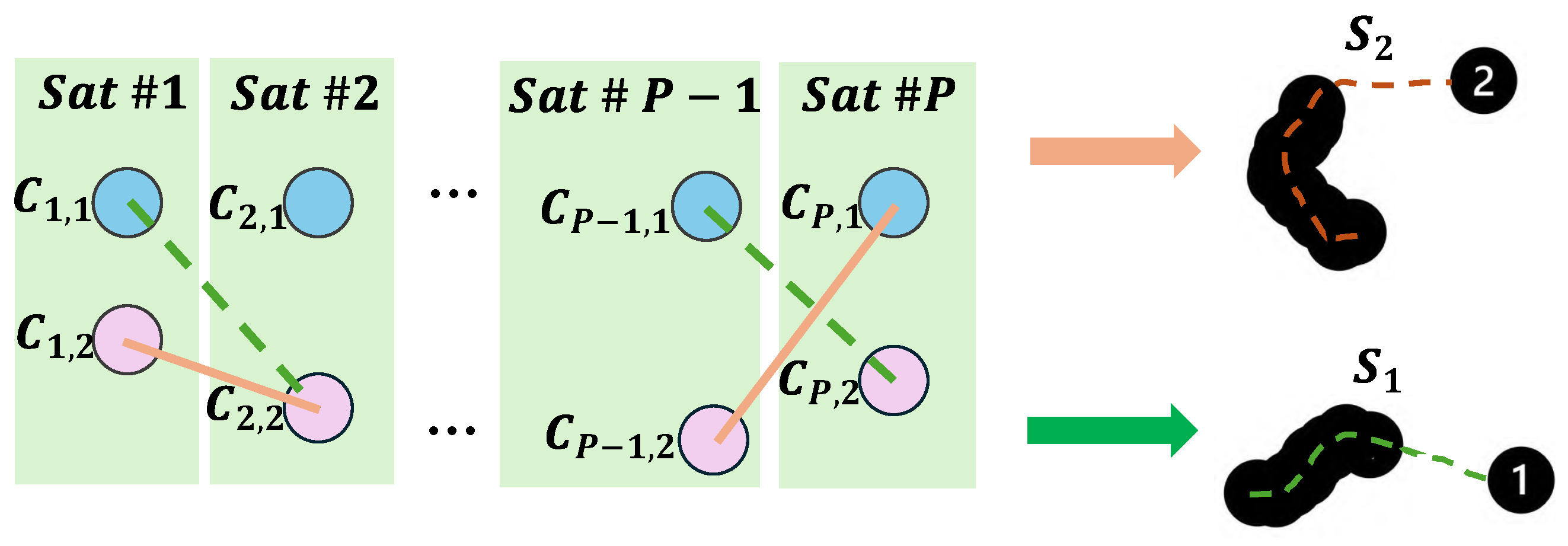
3.4. Position Recovery

In the position recovery stage, by evaluating the position sets generated by different channel selection schemes, we identify specific channels that only track the authentic component ${\mathit{y}}_{\mathrm{A}}$ of each satellite. The results can be extended to guarantee an accurate position solution.

First, one channel is selected from each channel pair $[C_{\mathrm{p},1},C_{\mathrm{p},2}]$ which has completed tracking. In total, $\mathrm{P}-1$ channels are chosen from all P channel pairs. Therefore, the channel selection scheme $G_g=[C_{1,\mathrm{x}},C_{2,\mathrm{x}},\dots ,C_{\mathrm{P}·2^{\mathrm{P}-1},x}]$, where $x=1$ or 2, has a total of ${\mathbf{C}}_{\mathrm{P}}^{\mathrm{P}-1}{\left({\mathbf{A}}_2^1\right)}^{\mathrm{P}-1}=\mathrm{P}·2^{\mathrm{P}-1}$ possibilities. Then, each channel selection scheme $G_g$ produces different pseudo-ranges for each satellite. Different channel selection schemes result in varying pseudo-ranges for each satellite. Finally, during the receiver’s PVT estimation stage, the Extended Kalman Filter (EKF) is applied to integrate these pseudo-ranges, yielding varying position results.

Because the receiver calculates position periodically, each $G_g$ produces different position trajectories over time. These trajectories, representing discrete position solutions, form unique sets. In Figure 6, each set is labeled $S_i$, where $i=1,2,\dots ,\mathrm{P}·2^{\mathrm{P}-1}$ corresponds to a particular channel selection scheme; thus, there are $\mathrm{P}·2^{\mathrm{P}-1}$ distinct sets, with each set representing a specific selection scheme. Among all these selection schemes, there exist three different scenarios:

(1)

Authentic selection schemes (P sets): Composed of channels that exclusively track genuine signals; when $\mathrm{P}>4$, these sets tend to produce consistent position results.

(2)

Fake selection schemes (P sets): Made up of channels that only track spoofed signals; these sets exhibit varied position outcomes due to the spoofing signals’ inability to continuously generate drag-off phases while simultaneously ensuring a uniform position across all satellites.

(3)

Mixed selection schemes ($\mathrm{P}·(2^{\mathrm{P}-1}-2)$ sets): Consisting of channels tracking both genuine and spoofed signals, the position results from these sets also vary significantly.

Collectively, there are P overlapping position sets $S_i$, corresponding to authentic position solutions generated by authentic selection schemes. The remaining position sets produced by fake and mixed schemes are scattered, with relatively large distances between them.

In order to range the distance and compare the similarity between two sets between different position sets, the Hausdorff distance $d_{\mathrm{H}}$ [26] is adopted. Let the bth and cth channel selection scheme corresponds to position set $S_b$ and $S_c$, respectively, where $b,c=1,2,\dots ,\mathrm{P}·2^{\mathrm{P}-1}$ and $b\ne c$. Then, the Hausdorff distance between $S_b$ and $S_c$ is defined as

$$\begin{array}{c}\hfill d_{\mathrm{H}}(S_b,S_c)=max\left\{h\left(S_b,S_c\right),h\left(S_c,S_b\right)\right\},\end{array}$$

while the shortest distance $h\left(S_b,S_c\right)$ from $S_b$ to $S_c$ is

$$\begin{array}{c}\hfill h\left(S_b,S_c\right)=max\{min\left\{d(p_{\mathrm{b}},p_{\mathrm{c}})\right|p_{\mathrm{b}}\in S_b\},p_{\mathrm{c}}\in S_c\},\end{array}$$

where $p_{\mathrm{b}}$ and $p_{\mathrm{c}}$ are arbitrary points in $S_b$ and $S_c$, respectively, and $d\left(p_{\mathrm{b}},p_{\mathrm{c}}\right)$ represents the distance between any two points in $S_b$ and $S_c$.

To evaluate the similarity between two different output result sets, we normalize the Hausdorff distance between any two candidate sets $S_b$ and $S_c$ by dividing it by the maximum pairwise distance:

$${\tilde{d}}_{\mathrm{H}}(S_b,S_c)={\displaystyle \frac{d_{\mathrm{H}}(S_b,S_c)}{{\max }_{b\ne c}{d}_{\mathrm{H}}(S_b,S_c)}}.$$

(21)

A normalized threshold $D_{thre}$ is then applied to determine valid overlaps. If ${\tilde{d}}_{\mathrm{H}}(S_b,S_c)$ between $S_b$ and $S_c$ is less than $D_{thre}$, then sets $S_b$ and $S_c$ are considered to overlap approximately. By calculating the Hausdorff distance $d_{\mathrm{H}}$ between each pair of sets, a distance matrix F can be constructed as

$$\begin{array}{c}\hfill F=\left[\begin{array}{ccc}{\tilde{d}}_{\mathrm{H}}\left(1,1\right)& \dots & {\tilde{d}}_{\mathrm{H}}\left(1,\mathrm{P}·2^{\mathrm{p}-1}\right)\\ {\tilde{d}}_{\mathrm{H}}\left(2,1\right)& \dots & {\tilde{d}}_{\mathrm{H}}\left(2,\mathrm{P}·2^{\mathrm{p}-1}\right)\\ ⋮& \ddots & ⋮\\ {\tilde{d}}_{\mathrm{H}}\left(\mathrm{P}·2^{\mathrm{p}-1},1\right)& \dots & {\tilde{d}}_{\mathrm{H}}\left(\mathrm{P}·2^{\mathrm{p}-1},\mathrm{P}·2^{\mathrm{p}-1}\right)\end{array}\right]\end{array}.$$

(22)

As shown in Figure 7, the distance matrix F is symmetric, and each row (or column) of matrix F corresponds to the normalized distance ${\tilde{d}}_{\mathrm{H}}$ between the current set of positions and other sets of positions. By identifying the gth row (or column)

$$\begin{array}{c}\hfill F(g,:)=\left[{\tilde{d}}_{\mathrm{H}}(g,1),\dots ,{\tilde{d}}_{\mathrm{H}}(g,\mathrm{P}·2^{\mathrm{P}-1})\right]\mathrm{or}F(:,g)=\left[{\tilde{d}}_{\mathrm{H}}(1,g),\dots ,{\tilde{d}}_{\mathrm{H}}(\mathrm{P}·2^{\mathrm{P}-1},g)\right]\end{array}$$

with the maximum number of overlapping sets, all channels included in the gth selection scheme $G_g$ are able to track the true signal, thereby obtaining the correct position solution $S_g$ for the receiver.

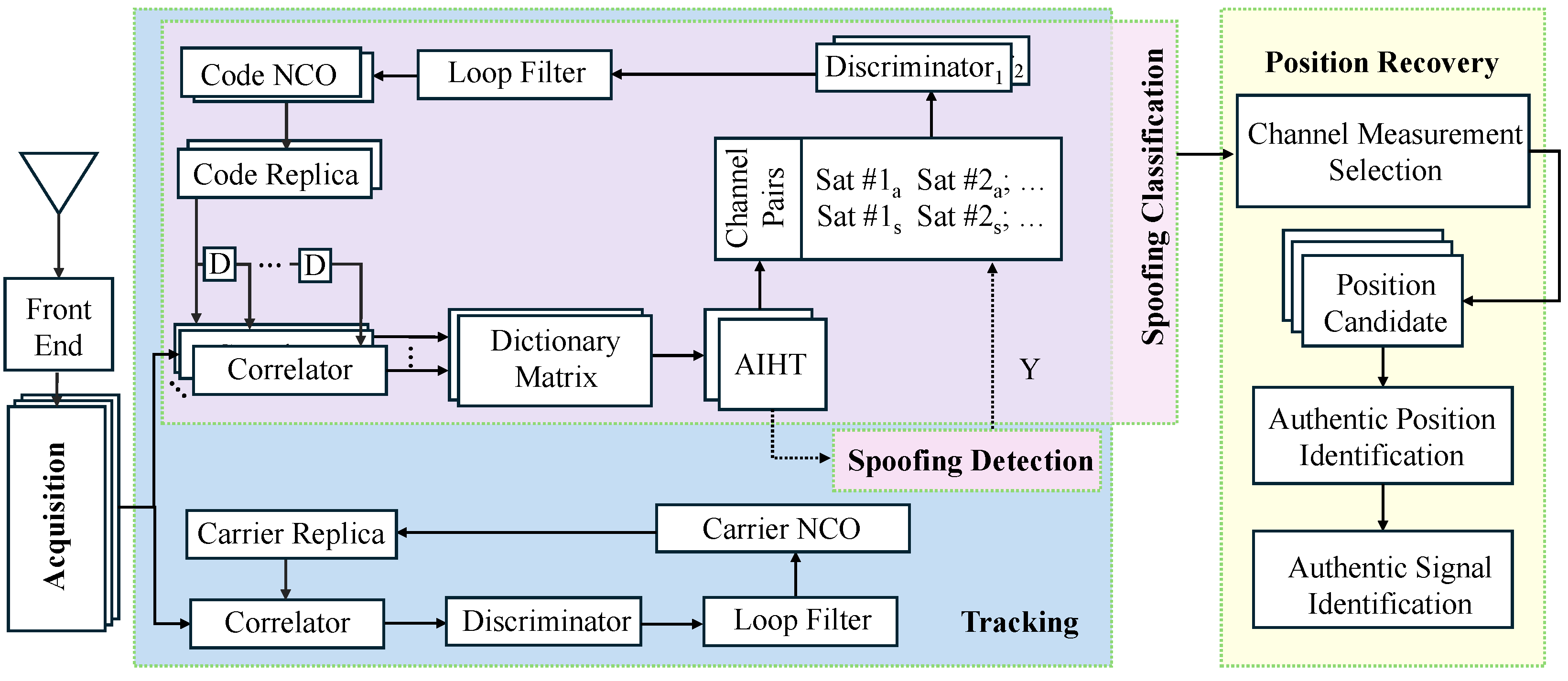
3.5. System Overview

Collectively, the pseudocode of implementation for the proposed spoofing detection, classification and position recovery algorithm is summarized in Algorithm 1. Under different channel selection schemes, the receiver’s operating state can be analyzed as follows:

• If our algorithm is initiated before spoofing attacks, it confirms that the target receiver is not under spoof, and no further steps are implemented unless the outcome of the AIHT algorithm suggests an opposite decision.
• If our algorithm is run after spoofing attacks, the receiver switches to alarm mode to perform classification and position recovery. The authentic position solution $S_g$ is identified by selecting the gth row (or column) of the distance matrix F with the highest number of overlapping sets.

Thus, from the process in Algorithm 1, it can be found that there is no limitation in the start time when applying our algorithm.

In the following, we further analyze the computational complexity in Algorithm 1 to illustrate the practicality of our results. Recall that the signal data length J and P satellites can be tracked, the computational complexity of the tracking loops is $O(\mathrm{P}\times \mathrm{J})$, and the AIHT’s complexity mirrors that of the conventional IHT algorithm, which is $O(\mathrm{K}\times \mathrm{N})$. Consequently, the cumulative complexity of the proposed AIHT algorithm before position recovery amounts to $O(\mathrm{P}\times \mathrm{K}\times \mathrm{N}\times \mathrm{J})$. In the position recovery process, assuming that the EKF operation of the PVT estimation has a computational complexity of $O\left(\mathrm{E}\right)$, the iterative process is conducted $(\mathrm{P}\times (2\mathrm{P}-1\left)\right)$ times in various channel selections, and a pair of tracking loops needs to be calculated for each satellite. Thus, the computational complexity post-spoofing detection is $O(\mathrm{P}\times \mathrm{K}\times \mathrm{N}\times \mathrm{J})+O(\mathrm{P}\times (2\mathrm{P}-1)\times \mathrm{E})$, which can be run by most commercial GNSS receivers.

Algorithm 1: The proposed spoofing detection, classification and position recovery algorithm.

Input: Satellite number P, correlation outputs ${\mathit{y}}_{\mathrm{p}}$, prior coefficient level K, reconstruction error $\epsilon$, threshold $T_{\mathrm{th}}$ and $D_{thre}$. Output: Receiver state, selection scheme $G_g$ of ($F(g,:)$) or column ($F(:,g)$) in F. 1: Initializing $2\mathrm{P}$ digital channels 2: while$t<t_{\mathrm{end}}$do 3:     if No spoofing signals are detected then 4:         for $\mathrm{p}=1,2,\dots ,\mathrm{P}$ do 5:            Initializing dictionary $\mathit{Q}$ 6:            while $\left({∥{\mathit{y}}_{\mathrm{p}}-\mathit{Q}{\mathit{\beta }}^{+}∥}_2^2>\epsilon \right)$ do 7:                ${\widehat{\mathit{\beta }}}^{+}=\underset{{\mathit{\beta }}^{+}}{\mathrm{argmin}}{∥\mathit{y}-\mathit{Q}{\mathit{\beta }}^{+}∥}_2^2,s.\mathrm{t}.\left({∥\mathit{\beta }∥}_0\le \mathrm{K}\right)$ 8:            end while 9:            if $\nexists {\mathit{\beta }}_{\mathrm{i}}$ which ${\mathit{\beta }}_i\ge T_{\mathrm{th}}$ then 10:                No existence of spoofing. 11:            else if $\exists {\mathit{\beta }}_{\mathrm{i}}$,${\mathit{\beta }}_{\mathrm{j}}$ which ${\mathit{\beta }}_{\mathrm{i}}$,${\mathit{\beta }}_{\mathrm{j}}\ge T_{\mathrm{th}}$ then 12:                Receiver under spoofing attack 13:            end if 14:         end for 15:     else 16:         if $\mathrm{P}>4$ then 17:            Activating position recovery 18:            for $\mathrm{p}=1,2,\dots ,\mathrm{P}$ do 19:                Obtaining corrected ${\widehat{{\mathit{y}}_{\mathrm{p}}}}_{\mathrm{i}}$, ${\widehat{{\mathit{y}}_{\mathrm{p}}}}_{\mathrm{j}}$ by AIHT-based APT method 20:                Tracking ${\widehat{{\mathit{y}}_{\mathrm{p}}}}_{\mathrm{i}}$ and ${\widehat{{\mathit{y}}_{\mathrm{p}}}}_{\mathrm{j}}$ within channel pair $[C_{\mathrm{p},1}$ and $C_{\mathrm{p},2}]$ 21:            end for 22:            Form selection scheme ${\mathrm{G}}_g$ from different channel pairs $G_r=[C_{1,\mathrm{x}},C_{2,\mathrm{x}},\dots ,C_{\mathrm{P}·2^{\mathrm{P}-1},x}],x\in \{1,2\}$ 23:         end if 24:     end if 25: end while 26: for$r=1,2,\dots ,\mathrm{P}·2^{\mathrm{P}-1}$do 27:     Form position set $S_r$ under scheme $G_r$ 28:     Calculate $F(r,:)$ or $F(:,r)$ 29: end for 30: Form the matrix F 31: Identify vector $F(g,:)$ or $F(:,g)$ with each normalized elements smaller than $D_{thre}$.

4. Experimental Results

In this section, we consider a GNSS receiver which suffers from spoofing attacks. The proposed anti-spoofing algorithm in Algorithm 1 is deployed to achieve spoofing detection, classification, and position recovery. The public TEXBAT dataset provided by the University of Texas at Austin containing GPS L1 base-band spoofing data [21,27] is utilized in the experiments. The dataset is postprocessed using FGI-GSRx, which is an open-source GPS software-defined receiver (SDR) developed by the Finnish Geospatial Research Institute (FGI) [28]. Extensive experiments are conducted to fully illustrate the efficiency and advantages of each stage of the proposed spoofing algorithm.

4.1. Performance Analysis of AIHT Algorithm

In this subsection, scenario 4 in TEXBAT is utilized to evaluate the proposed AIHT detection algorithm’s performance. As shown in Figure 8, the spoofing attack begins to distort the channel at the 190-s mark.

Moreover, to illustrate the efficiency and advantage of our algorithm, we further analyze it in comparison with some related methods, including a traditional IHT algorithm [25] and a Least Absolute Shrinkage and Selection Operator (LASSO)-based spoofing detection algorithm [10].

Figure 9a compares the detection accuracy of our AIHT algorithm against the conventional IHT and LASSO methods. To achieve 90% accuracy, AIHT can detect spoofing for delays as small as $\Delta \tau >0.71$ chips, whereas both IHT and LASSO require $\Delta \tau >0.8$ chips under the same criterion. Figure 9b displays the root mean square error (RMSE) between $\mathit{y}$ and the reconstructed result $\widehat{\mathit{y}}$ under different algorithms. Collectively, the proposed AIHT algorithm not only maintains a satisfying detection rate in a small code phase gap between the authentic and spoofing peak components, it also has the smallest reconstruction error, implying outstanding ability to recognize the corresponding code phases ${{\widehat{\mathit{\beta }}}_{\mathrm{i}}}^{+}$ and ${{\widehat{\mathit{\beta }}}_{\mathrm{j}}}^{+}$ of different signal components.

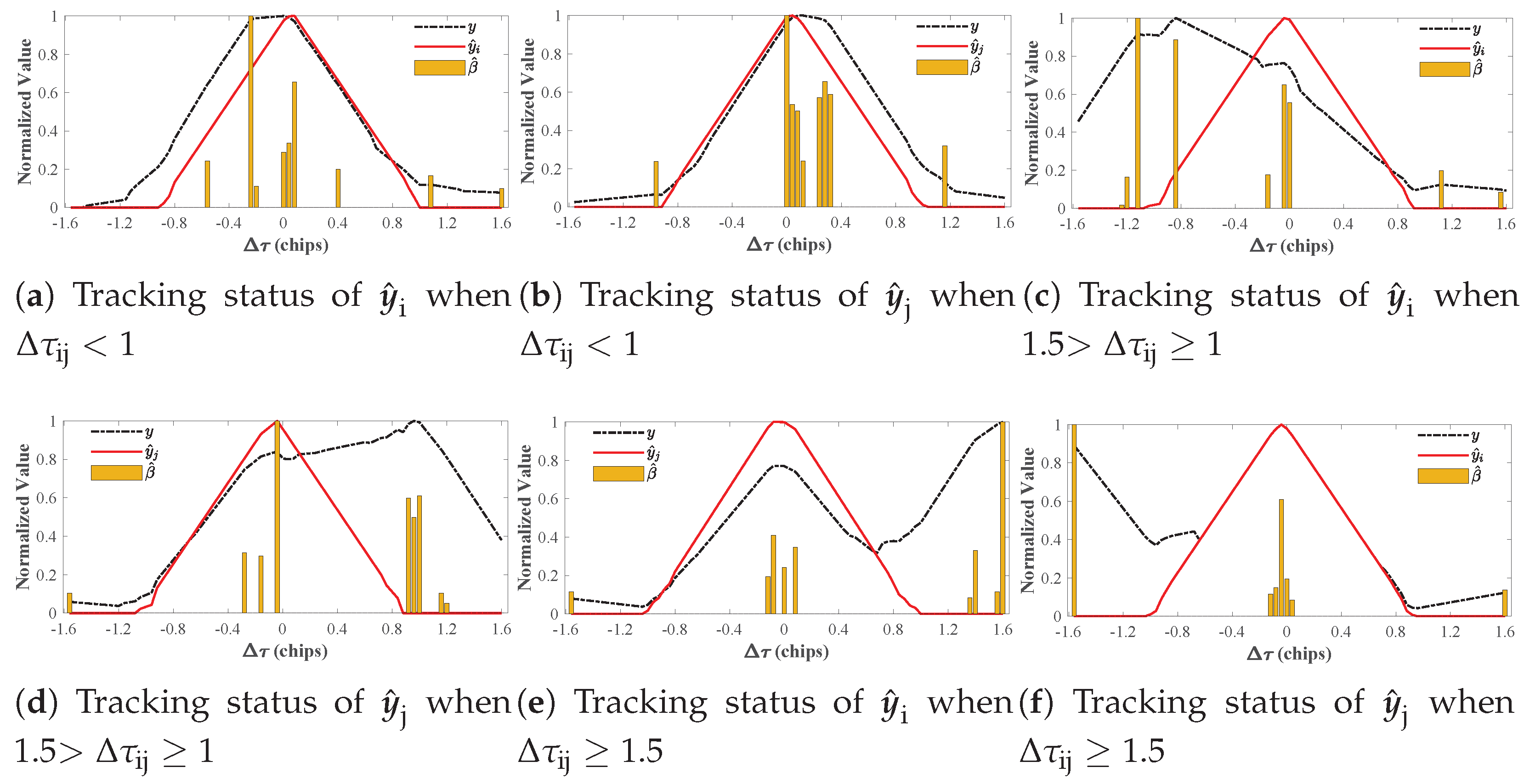
4.2. Robustness Analysis of DLL Under AIHT-Based APT Algorithm

In this section, the fluctuation of the DLL is analysed over different time periods to evaluate the stability of DLL loop calibration under our AIHT-based APT algorithm. Again, we use scenario 4 in the TEXBAT dataset.

As shown in Figure 10, during the time periods of 195–215 s, 220–250 s and 250–280 s, the oscillation amplitude ${\mathrm{DLL}}_{\mathrm{err}}$ decreases and the DLL loop tends to stabilize after tracking and alignment with the target signal component ${\widehat{\mathit{y}}}_{\mathrm{i}}$ or ${\widehat{\mathit{y}}}_{\mathrm{j}}$. Upon detection of spoofing signals, AIHT-based APT algorithm begins. Figure 11 depicts the actual DLL correction process of the proposed AIHT-based APT algorithm for different values of $\Delta {\tau }_{\mathrm{ij}}$. The tracking process in channels $C_{\mathrm{p},1}$ and $C_{\mathrm{q},1}$, illustrated in Figure 11a,c, respectively, gradually locks onto ${\widehat{\mathit{y}}}_{\mathrm{i}}$, while the tracking process in channels $C_{\mathrm{p},2}$ and $C_{\mathrm{q},2}$, detailed in Figure 11b,d, respectively, gradually locks onto ${\widehat{\mathit{y}}}_{\mathrm{j}}$, $p\ne q$.

The tracking adjustments depicted in Figure 11 correlate with changes in the discriminator of the DLL, as shown in Figure 10. When the initial correlation peak is not the one the channel is designated to lock onto, ${\mathrm{DLL}}_{\mathrm{err}}$ undergoes significant adjustments to shift from initially aligning with $\widehat{\mathit{y}}$ to the calibrated components ${\widehat{\mathit{y}}}_{\mathrm{i}}$ or ${\widehat{\mathit{y}}}_{\mathrm{j}}$. Upon successful re-locking onto the correct peak, ${\mathrm{DLL}}_{\mathrm{err}}$ diminishes and approaches zero.

As shown in Figure 12, different signal components of the channel pair $\left([C_{p,1},C_{p,2}]\right)$ are stably tracked and calibrated, with the DLL loop aligned precisely to the assigned correlation peak $\left({\widehat{\mathit{y}}}_i\right)$ or $\left({\widehat{\mathit{y}}}_j\right)$. Figure 12a,b illustrates the channel pair when the code phase difference $(\Delta {\tau }_{ij})$ is less than 1.

Figure 12c,d shows the channel pair for $(1.5>\Delta {\tau }_{ij}\ge 1)$, while Figure 12e,f depicts the channel pair for $(\Delta {\tau }_{ij}\ge 1.5)$. These figures emphasize the efficacy of AIHT-driven code phase estimations in achieving independent channel adjustments within a channel pair, ensuring stable AIHT-based APT tracking and minimizing fluctuations in subsequent position recovery.

4.3. Evaluation of the Receiver’s Position Recovery Results

In this section, the position recovery performance of our algorithm is fully evaluated under the scenario 4 in TEXBAT, where the spoofing attack is initiated at 190 s and gradually introduces a 600 m erroneous position offset in the earth-centered earth-fixed (ECEF) coordinates. The true coordinates of the receiver in the WGS84 coordinate system are known to be latitude ${30}^{\circ }{17}^{\prime }15.{068}^{\prime \prime }N$, longitude ${97}^{\circ }{44}^{\prime }08.{642}^{\prime \prime }E$, and altitude 170 m.

Figure 13 illustrates the different position results obtained by proposed spoofed measurement mitigation algorithm discussed in Section 3.4 for different channel selections among all channel pairs, from the 300 s to the 350 s. Because the receiver in scenario 4 can receive $P=7$ satellites, there are a total of ${\mathbf{C}}_P^{P-1}{\left({\mathit{A}}_2^1\right)}^{P-1}=448$ position sets for different channel results.

As shown in Equation (22), $d_{\mathrm{H}}$ is calculated between each pair of the 448 position sets, resulting in a $448\times 448$ matrix F. Setting the threshold $T_{\mathrm{th}}=50$%, $D_{\mathrm{Thre}}=8$%, the search for the rows $F(g,:)$ (or columns $F(:,g)$) with the most overlaps in matrix F allows for the selection of eight sets of approximately overlapping position trajectories, namely, ${\sum }_{1<i<448}{d}_{\mathrm{H}}(\mathrm{i},g)<D_{Thre}$, which are regarded as the true position solution $S_g$ of the target receiver. Based on these approximately overlapping position sets and the corresponding channel selections, channel identification for tracking the true component in $\left[C_{\mathrm{p},1},C_{\mathrm{p},2}\right]$ can be achieved.

Figure 14, Figure 15 and Figure 16 illustrate the identification results of the position recovery trajectories and dimensional position error of the position recovery algorithm in different time periods.

Figure 14 shows that when the proposed spoofing countermeasure is applied before the spoofing attack begins, the recovered position error (red line) overlaps with the spoofed position error in the early stages before detection, as compared to Figure 8; afterwards, the proposed sensitive AIHT algorithm enables early detection and recovery, stabilizing the receiver’s trajectory and preventing significant deviations in the position results. Figure 15 and Figure 16 display the trajectories and position errors from 245 s to 343 s when $\Delta {\tau }_{\mathrm{ij}}\le 1$ and from 275 s to 378 s when $\Delta {\tau }_{\mathrm{ij}}>1$, respectively. These figures demonstrate that significant position resolution deviations are corrected by the position recovery algorithm, effectively realigning the position to the true values in different time periods.

To evaluate the stability of our position recovery algorithm, we compute the RMSE over different time periods in both static (scenario 4) and dynamic (scenario 6) environments.

Table 1. RMSE (m) under our position recovery algorithm across different time periods after deployment. The values represent the RMSE for two different scenarios: scenario 4 (first value) and scenario 6 (second value).

$\mathit{\Delta }{\mathit{\tau }}_{\mathbf{ij}}$ (chip)	Direction	RMSE (m)
		0 s–80 s	80 s–end
non-spoofing	X	14.4, 159.1	4.9, 9.3
	Y	25.6, 18.1	7.0, 8.2
	Z	17.5, 49.8	6.1, 8.3
$\Delta {\tau }_{\mathrm{ij}}\le 1$	X	37.8, 349.4	3.7, 9.4
	Y	33.4, 76.6	5.3, 10.1
	Z	71.6, 222.4	6.4, 9.8
$\Delta {\tau }_{\mathrm{ij}}>1$	X	13.1, 527.1	3.2, 7.4
	Y	34.7, 82.3	14.1, 11.9
	Z	62.4, 187.8	6.2, 10.1

lists the RMSE values in the X, Y, and Z dimensions of the ECEF coordinate system during various phases of recovery. As shown in Figure 14b–Figure 16b, the algorithm initially shows fluctuations for the first 80 s after deployment, which then stabilize until the end. The RMSEs for the time periods before and after 80 s from deployment are calculated and presented in Table 1. Scenario 6 shows a larger RMSE than scenario 4 during the first 80 s because the spoofing attack shifts the receiver farther away; in later stages, the RMSE decreases but remains slightly higher than in scenario 4, which is due to the stronger spoofing power causing the receiver to track the spoofed signals more persistently. We further analyze performance across different spoofing delays $\Delta {\tau }_{\mathrm{ij}}$. As indicated in Table 1, our method performs effectively for both $\Delta {\tau }_{\mathrm{ij}}\le 1$ and $\Delta {\tau }_{\mathrm{ij}}>1$, with satisfyingly low RMSE during the stabilized recovery stages from 80 s to the end of the recovery algorithm. It is worth mention that the higher Y-axis RMSE under $\Delta {\tau }_{\mathrm{ij}}>1$ in scenario 4 results from unstable code phase estimates during the spoofing-dominant phase. This instability is primarily caused by loop noise, which particularly affects satellites contributing along the Y-axis.

5. Discussion

The two main objectives of this article are to achieve accurate detection of spoofing interference and to ensure stable position recovery results under different spoofing conditions. To achieve the first objective, as discussed in Section 4.1, spoofing detection accuracy is evaluated by comparing the RMSE between $\mathit{y}$ and the $\widehat{\mathit{y}}$ reconstructed by the proposed AIHT-based detection method and other algorithms, for which we use publicly available datasets across several different scenarios. For the second objective, as outlined in Section 4.2, the effectiveness of the position recovery algorithm is indirectly evaluated by analyzing the tracking performance of each channel pair during the classification phase. Because smaller DLL discriminator fluctuations indicate a more stable AIHT-based APT algorithm, Figure 10, Figure 11, Figure 12 and Figure 13 show that the discriminator quickly regains stability during loop correction, validating the potential for successful position recovery.

The experiments in Section 4.3 visually demonstrate the effectiveness and stability of the proposed position recovery algorithm. Figure 14, Figure 15 and Figure 16 and Table 1 show that the proposed spoofing detection, classification, and position recovery algorithm effectively mitigates the impact of spoofing interference across various scenarios both before and during spoofing attacks on the receiver while maintaining stable recovery results.

To validate the sensitivity of $D_{thre}$, we vary its value and check whether the proposed positioning recovery method still correctly selects the authentic scheme with the maximum number of overlapping sets in matrix F. For Scenario 4, $D_{thre}$ values between 6% and 10% are effective, as shown in Figure 17a,b. When $D_{thre}$ exceeds 10%, the number of overlaps from the authentic selection scheme no longer increases, as all relevant sets are already included; meanwhile, overlaps from fake or mixed schemes continue to grow. Therefore, if $D_{thre}$ becomes too large, the recovery algorithm may mistakenly treats spoofed channels as authentic, leading to positioning errors. Similarly, for scenario 6, $D_{thre}$ values between 4% and 9% are effective. Based on both cases, we set $D_{thre}=8\%$ in our implementation.

Compared to prior approaches such as [5,20], our method introduces fewer assumptions and demonstrates better adaptability under challenging spoofing conditions. The CADLL-based method in [5] requires a stable initialization from a preceding MEDLL stage. If spoofing has already started before the receiver begins tracking, the loop fails to converge and the system may diverge. The MLE-based estimator in [20] assumes that the spoofing delay exceeds 0.75 chips. When this condition is not met, the estimation matrix becomes ill-conditioned, often resulting in severe estimation errors. In contrast, our method neither depends on prior authentic tracking states nor requires a minimum spoofing delay. Through sparse decomposition and iterative recovery, it can resolve closely spaced correlation peaks and remain effective even when the spoofing delay is small.

Importantly, we acknowledge a critical limitation of the proposed framework in that it requires at least five visible satellites (i.e., $p>4$) in order to construct a valid position recovery scheme. In urban canyon environments, this condition may not always be met. To handle such scenarios, a promising approach is to integrate signals from other systems, such as 5G localization or Low Earth Orbit (LEO)-based navigation. A recent study [15] has shown that 5G signals can enhance spoofing resistance when GNSS signals are degraded. Moreover, we are developing a custom-designed navigation signal for LEO dedicated positioning [2] to ensure robust performance under limited satellite visibility. Hybrid GNSS-LEO based anti-spoofing strategies will be explored in our future work.

6. Conclusions

This paper has investigated the issue of reliable and secure navigation for GNSS receivers subject to spoofing attacks. We propose a sparse decomposition algorithm with non-negative constraints limited by received signal power magnitudes, which not only achieve accurate spoofing detection but also extracts key features of the received signal’s contributing components. During the spoofing classification process, these features are utilized to continuously refine receiver’s code tracking loop in order to resist drag-off by the spoofed signal, ensuring that the contributing components of each spoofed satellite are tracked separately within channel pairs. Moreover, leveraging the inherent inconsistency of spoofing properties, we incorporate the Hausdorff distance to identify the most overlapped position sets, enabling the determination of genuine position trajectories and effectively mitigating the impacts of spoofing. The key advantage of our anti-spoofing framework is its ability to continuously track all contributing components of received signals and further exploit the inherent inconsistency of spoofing signals, which eliminates the need for extra devices or specific initial conditions. The efficiency and advantages of the proposed anti-spoofing framework are fully illustrated through extensive experimental studies conducted on the public TEXBAT dataset.

References

1. Kaplan, E.D.; Hegarty, C. Understanding GPS/GNSS: Principles and Applications; Artech House: Norwood, MA, USA, 2017. [Google Scholar]
2. He, Y.; Zhuang, X.; Hou, Y.; Wu, L. Robust blind space-time adaptive processing for measurement error mitigation in GNSS receivers. IET Commun. 2023, 17, 1021–1036. [Google Scholar] [CrossRef]
3. Bhatti, J.; Humphreys, T.E. Hostile control of ships via false GPS signals: Demonstration and detection. Navig. J. Inst. Navig. 2017, 64, 51–66. [Google Scholar] [CrossRef]
4. Guo, Y.; Wu, M.; Tang, K.; Tie, J.; Li, X. Covert spoofing algorithm of UAV based on GPS/INS-integrated navigation. IEEE Trans. Veh. Technol. 2019, 68, 6557–6564. [Google Scholar] [CrossRef]
5. Wang, Y.; Kou, Y.; Huang, Z.; Zhao, Y. GNSS spoofing maximum-likelihood estimation switching between MEDLL and CADLL. GPS Solut. 2023, 27, 148. [Google Scholar] [CrossRef]
6. Psiaki, M.L.; Humphreys, T.E. GNSS spoofing and detection. Proc. IEEE 2016, 104, 1258–1270. [Google Scholar] [CrossRef]
7. Zhou, Z.; Li, H.; Chen, Z.; Lu, M. Velocity Consistency Checking based GNSS Spoofing Detection Method for Vehicles. IEEE Trans. Veh. Technol. 2023. [Google Scholar] [CrossRef]
8. Fang, J.; Yue, J.; Xu, B.; Hsu, L.T. A post-correlation graphical way for continuous GNSS spoofing detection. Measurement 2023, 216, 112974. [Google Scholar] [CrossRef]
9. Sun, C.; Cheong, J.W.; Dempster, A.G.; Zhao, H.; Bai, L.; Feng, W. Robust spoofing detection for GNSS instrumentation using Q-channel signal quality monitoring metric. IEEE Trans. Instrum. Meas. 2021, 70, 8504115. [Google Scholar] [CrossRef]
10. Schmidt, E.; Gatsis, N.; Akopian, D. A GPS spoofing detection and classification correlator-based technique using the LASSO. IEEE Trans. Aerosp. Electron. Syst. 2020, 56, 4224–4237. [Google Scholar] [CrossRef]
11. Wang, H.; Li, H.; Zhong, M.; Lu, M. A Space-Time-Ambiguity Decomposition Method for DOA Estimation Enhancing Anti-Spoofing Via Rotating Dual Antennas. IEEE Trans. Aerosp. Electron. Syst. 2024, 60, 7643–7662. [Google Scholar] [CrossRef]
12. He, L.; Li, H.; Lu, M. Dual-antenna GNSS spoofing detection method based on Doppler frequency difference of arrival. Gps Solut. 2019, 23, 78. [Google Scholar] [CrossRef]
13. Shang, X.; Sun, F.; Liu, B.; Zhang, L.; Cui, J. GNSS Spoofing Mitigation With a Multicorrelator Estimator in the Tightly Coupled INS/GNSS Integration. IEEE Trans. Instrum. Meas. 2022, 72, 2529013. [Google Scholar] [CrossRef]
14. Kujur, B.; Khanafseh, S.; Pervan, B. Optimal INS Monitor for GNSS Spoofer Tracking Error Detection. Navig. J. Inst. Navig. 2024, 71, navi.629. [Google Scholar] [CrossRef]
15. Bai, L.; Sun, C.; Dempster, A.G.; Zhao, H.; Feng, W. GNSS Spoofing Detection and Mitigation With a Single 5G Base Station Aiding. IEEE Trans. Aerosp. Electron. Syst. 2024, 60, 4601–4620. [Google Scholar] [CrossRef]
16. Kujur, B.; Khanafseh, S.; Pervan, B. Detecting GNSS spoofing of ADS-B equipped aircraft using INS. In Proceedings of the 2020 IEEE/ION Position, Location and Navigation Symposium (PLANS), Portland, OR, USA, 20–23 April 2020; pp. 548–554. [Google Scholar] [CrossRef]
17. Kuusniemi, H.; Blanch, J.; Chen, Y.H.; Lo, S.; Innac, A.; Ferrara, G.; Honkala, S.; Bhuiyan, M.Z.H.; Thombre, S.; Söderholm, S.; et al. Feasibility of fault exclusion related to advanced RAIM for GNSS spoofing detection. In Proceedings of the 30th International Technical Meeting of the Satellite Division of the Institute of Navigation (ION GNSS+ 2017), Portland, OR, USA, 25–29 September 2017; pp. 2359–2370. [Google Scholar]
18. Zhou, W.; Lv, Z.; Wu, W.; Shang, X.; Ke, Y. Anti-spoofing technique based on vector tracking loop. IEEE Trans. Instrum. Meas. 2023, 72, 8504516. [Google Scholar] [CrossRef]
19. Xu, B.; Jia, Q.; Hsu, L.T. Vector tracking loop-based GNSS NLOS detection and correction: Algorithm design and performance analysis. IEEE Trans. Instrum. Meas. 2019, 69, 4604–4619. [Google Scholar] [CrossRef]
20. Shang, X.; Sun, F.; Zhang, L.; Cui, J.; Zhang, Y. Detection and mitigation of GNSS spoofing via the pseudorange difference between epochs in a multicorrelator receiver. Gps Solut. 2022, 26, 37. [Google Scholar] [CrossRef]
21. Humphreys, T.E.; Bhatti, J.A.; Shepard, D.; Wesson, K. The Texas Spoofing Test Battery: Toward a Standard for Evaluating GPS Signal Authentication Techniques; The University of Texas: Austin, TX, USA, 2012. [Google Scholar]
22. Mohimani, H.; Babaie-Zadeh, M.; Jutten, C. A fast approach for overcomplete sparse decomposition based on smoothed L0 norm. IEEE Trans. Signal Process. 2008, 57, 289–301. [Google Scholar] [CrossRef]
23. Blanchard, J.D.; Cermak, M.; Hanle, D.; Jing, Y. Greedy algorithms for joint sparse recovery. IEEE Trans. Signal Process. 2014, 62, 1694–1704. [Google Scholar] [CrossRef]
24. Foucart, S.; Lecué, G. An IHT algorithm for sparse recovery from subexponential measurements. IEEE Signal Process. Lett. 2017, 24, 1280–1283. [Google Scholar] [CrossRef]
25. Blumensath, T.; Davies, M.E. Iterative hard thresholding for compressed sensing. Appl. Comput. Harmon. Anal. 2009, 27, 265–274. [Google Scholar] [CrossRef]
26. Huttenlocher, D.P.; Klanderman, G.A.; Rucklidge, W.J. Comparing images using the Hausdorff distance. IEEE Trans. Pattern Anal. Mach. Intell. 1993, 15, 850–863. [Google Scholar] [CrossRef]
27. Humphreys, T. TEXBAT Data Sets 7 and 8; The University of Texas: Austin, TX, USA, 2016. [Google Scholar]
28. Söderholm, S.; Bhuiyan, M.Z.H.; Thombre, S.; Ruotsalainen, L.; Kuusniemi, H. A multi-GNSS software-defined receiver: Design, implementation, and performance benefits. Ann. Telecommun. 2016, 71, 399–410. [Google Scholar] [CrossRef]
Figure 1. Different stages of spoofing signals attempting to take control of DLLs, where y , y A , and y S are depicted in the red, blue, and green triangles, respectively.
Remotesensing 17 02703 g001
Figure 2. Flowchart of the proposed spoofing detection, classification, and position recovery algorithm.
Remotesensing 17 02703 g002
Figure 3. Dictionary matrix Q construction.
Remotesensing 17 02703 g003
Figure 4. Comparison of reconstruction performance between the conventional IHT algorithm and the proposed AIHT algorithm.
Remotesensing 17 02703 g004
Figure 5. The early (E), prompt (P) and late (L) values selected by the DLL; here, δ E L means the early–late separation.
Remotesensing 17 02703 g005
Figure 6. Formation of distinct position sets S i based on different channel selection schemes.
Remotesensing 17 02703 g006
Figure 7. Distance matrix F with color-coded elements: blue for values below D t h r e and yellow for values above.
Remotesensing 17 02703 g007
Figure 8. Position results of a GNSS receiver under spoofing interference in scenario 4 of the TEXBAT dataset.
Remotesensing 17 02703 g008
Figure 9. Comparison of spoofing detection accuracy and reconstruction RMSE across algorithms for various code phase intervals.
Remotesensing 17 02703 g009
Figure 10. The oscillation of DLLs induced by APT at different time intervals.
Remotesensing 17 02703 g010
Figure 11. Tracking status of the channel pair C p , 1 , C p , 2 when code interval Δ τ ij > 1 (a,b) and C q , 1 , C q , 2 when code interval Δ τ ij < 1 (c,d).
Remotesensing 17 02703 g011
Figure 12. Tracking status of the calibrated y ^ i and y ^ j after correction, with different code delays Δ τ ij between channels.
Remotesensing 17 02703 g012
Figure 13. Different position results for different channel selections.
Remotesensing 17 02703 g013
Figure 14. Three-dimensional trajectory and position error of spoofed and recovered navigation solutions from 160 s to 296 s.
Remotesensing 17 02703 g014
Figure 15. Three-dimensional trajectory and position error of spoofed and recovered navigation solutions from 245 s to 343 s.
Remotesensing 17 02703 g015
Figure 16. Three-dimensional trajectory and position error of spoofed and recovered navigation solutions from 275 s to 378 s.
Remotesensing 17 02703 g016
Figure 17. Overlapping set counts under varying normalized D t h r e values for the two different scenarios.
Remotesensing 17 02703 g017