1. Introduction
In underground mining, movements in the rock strata caused by ground movements, expansions, and other factors can lead to hazardous incidents such as rock falls. To mitigate such incidents, rock bolts, shotcrete linings, and steel meshes are used to support loose rock mass. Rock bolts are generally steel bars that are bolted into the weak rock strata to provide anchorage and strengthen their load-bearing capacity, hence providing structural support to the walls and roofs of the mine, thereby preventing it from collapsing [
1,
2]. Rock falls not only lead to disruptions in mining operations but also can cause fatal injuries and massive damage to mine infrastructure and ventilation systems. Various factors like improper installation, design, and physical changes due to natural as well as mining activities can lead to quality degradation and corrosion in rock bolts [
3]. Therefore, it is highly imperative to perform regular assessments of these rock bolts to avert any hazards. Manual investigations of rock bolts are performed by surveyors in underground mines, which is extremely time-consuming and challenging due to the low-light conditions in underground mines as well as limited due to restrictive mine access rules. On the other hand, instrumented rock bolts using sensors like strain gauges [
4], washer compression sensors [
5], load sensors, ultrasonic monitoring [
6], and fibre Bragg grating sensors [
7] serve as solutions to accurately monitor individual bolts [
2,
8]. However, to scale the rock bolt monitoring and visualisation process over vast sections of the mines, automated recognition of rock bolts using close-range remote sensing serves as a potential solution. Traditional surface mapping equipment, such as terrestrial laser scanners (TLSs), faces limitations from the absence of GNSS and restricted sensor mobility in underground environments [
9]. Sensor mobility is especially needed for scalability in underground mines, as static scanners can only gather data from a fixed vantage point, effectively seeing in one direction. While this may be suitable in open spaces, in underground mines, it results in limited coverage and occlusion of critical regions, restricting the ability to comprehensively map large, complex environments. Additionally, GNSS-based systems are unsuitable in underground environments because satellite signals cannot penetrate dense rock and overburden, preventing the receiver from establishing the satellite communication required for accurate positioning, making the system unscalable across large and complex tunnel networks. With recent advancements in mobile laser scanning and Simultaneous Localisation and Mapping (SLAM), the potential for large-scale 3D point cloud data acquisition in GNSS-denied underground mining sections like tunnels and roadways has been significantly enhanced [
10], paving the way for more efficient underground environment mapping and monitoring.
Martínez-Sánchez et al. [
11] presented one of the earliest studies incorporating rock bolt identification by registering initial and post-shotcrete point clouds using bolts as reference points. Although rock bolt detection was not their primary goal, their encoder model, comprising an output layer and two autoencoders, targeted bolt identification. To enable accurate shotcrete volume analysis, the method prioritised high recall over precision, leading to many false positives. Despite this trade-off, their work was the first to demonstrate the feasibility of using geometric neighbourhood-based machine learning algorithms for support structure monitoring challenges. In another study, Gallwey et al. [
12] explored the use of a machine learning-based approach to identify rock bolts in a point cloud obtained using a TLS. They generated a point descriptor comprising 65 features representing neighbourhood variations like eigenvalue and density-based features, for each point in the point cloud. To classify rock bolts, they tested a neural network and a random forest classifier and found the former to be more accurate. They trained their neural network model on the 65-dimensional classifier descriptor that they manually defined, rather than being learned by a deep neural network. Despite this limitation, they were able to achieve a respectable rock-bolt classification outcome, though point-wise performance still left room for improvement.
Using a wide array of features and point descriptors does not necessarily translate to a better classification result since many features might behave similarly for both bolts and non-bolts. For instance, eigenvalue-derived metrics like omnivariance can be prominent around both bolts and rock mass discontinuities, and features such as verticality are ineffective in distinguishing bolts [
12]. A different study by Singh et al. [
13] used selective point descriptors for rock bolt classification in an MLS-acquired point cloud of an underground mine. Exploiting the cylindrical nature of rock bolts in a point cloud, they used three descriptors, proportion of variance (PoV), radial surface descriptor (RSD), and fast point feature histogram (FPFH), to train their feed-forward artificial neural network (ANN) for rock bolt classification. Later, Saydam et al. [
14] proposed a bolt detection algorithm tailored for clean small-scale TLS point clouds of construction tunnels prior to shotcrete application, where environmental variability is minimal. Their method followed a coarse-to-fine strategy, initially using the proportion of variance (PoV) descriptor to roughly isolate potential bolt clusters. A neural network was then applied to each cluster, standardised to a fixed size, to distinguish bolt points from the background. This hierarchical approach significantly improved bolt detection precision, thanks to the initial filtering step. In another study, Singh et al. [
15] investigated a robust approach for rock bolt identification in MLS point cloud by first introducing a point cloud resampling pre-processing step using moving least squares to mitigate the noisy and sparse nature of an MLS point cloud. Following that, the approach uses a Canupo classifier trained on a multi-scale point descriptor comprising pointness, curveness, and surfaceness paired with the RANSAC shape detection algorithm. This approach effectively identified bolts by leveraging their cylindrical characteristics and separating them from surrounding mine surfaces.
Most research on rock bolt identification relies on feature engineering and traditional machine learning algorithms. Deep learning methods, on the other hand, offer greater flexibility by automatically learning complex features and typically achieve better performance in irregular geometries [
16], making them well-suited for underground mining environments. Although there has been significant progress in deep learning-based semantic segmentation of point clouds [
17,
18], limited research has been undertaken to utilise those models in the context of rock bolt identification and support structure mapping. Deep learning models have the inherent ability to identify feature vectors for associating classes and labels with points. Unlike other machine learning algorithms, they do not require manual feature definition. However, specific challenges arise when identifying small-scale objects, such as rock bolts, within large-scale point clouds from underground mines that need to be addressed in order to improve overall accuracy and efficiency.
To this end, this study proposes a novel deep learning architecture,
DeepBolt, for the automatic identification of rock bolts in medium- to large-scale complex 3D point clouds of underground mines captured using mobile laser scanners.
DeepBolt adopts a two-stage approach that combines a geometry-sensitive filtering strategy with a graph-based semantic segmentation model that dynamically constructs local graphs in feature space to capture both local and global geometric structures critical for accurate point-wise classification, as detailed in
Section 2. The proposed approach offers a robust and efficient solution to the unique problem of rock bolt identification, which includes severe class imbalance due to the small size of bolts relative to the scan area, data noise, and high environmental variability in real-world underground mining scenarios, and visibility of rock bolts due to face-plate obscurity caused by shotcrete application. To assess the performance of the proposed rock bolt identification approach, it is compared to the state-of-the-art semantic segmentation models and current rock bolt identification techniques, as discussed in
Section 3.
2. Materials and Methods
This section provides a description about the specifications of the 3D point cloud dataset, the technologies and sensors used for their acquisition from underground mines, the pre-processing and noise filtering steps used on the dataset, and the deep learning model used for rock bolt identification in the point cloud.
2.1. Mobile Laser Scanner
LiDAR used in underground mining can be bifurcated into two primary types: TLSs (terrestrial laser scanners) and MLSs (mobile laser scanners) [
9,
19,
20,
21]. A TLS scans the surrounding environment from a fixed point. An MLS, on the other hand, is generally handheld or vehicle-mounted and uses SLAM algorithms (Simultaneous Localisation and Mapping) for scanning. While the TLS offers millimetre-level accuracy from a stationary perspective, the MLS brings the advantage of mobility, albeit with a compromise in accuracy, which is mostly in centimetres, and increased susceptibility to noise. With increased mobility, an MLS has the potential to cut down on blind spots and occlusions, making it a great option for data collection in large-scale regions. Both TLSs and MLSs have their benefits, and the choice of laser scanner comes down to the application it is being used for.
In terrestrial laser scanning (TLS), the sensor remains stationary at a fixed location, capturing a 3D point cloud of the surrounding environment. In contrast, mobile laser scanning (MLS) involves a moving sensor, where both the sensor position and the environment are initially unknown. Consequently, MLS requires solving two problems: localisation and mapping. Simultaneous Localisation and Mapping (SLAM) addresses these by concurrently estimating the sensor pose and constructing the map. SLAM is particularly valuable for rapid mobile scanning in environments with limited or no GNSS availability, such as underground mines, by integrating inertial measurement unit (IMU) data with laser scans to reduce drift and uncertainty [
22]. Although SLAM enables efficient underground scanning, it is an optimisation problem that can accumulate position drifts over time, which can be mitigated using loop closure, a process that corrects accumulated drift by recognising previously scanned locations and aligning them accurately.
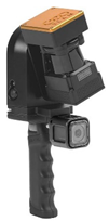
To collect medium- to large-scale data from underground mines, this study uses a handheld mobile laser scanner, Zeb-REVO, that addresses the challenges of immobility and occlusion in TLS data. The system (
Table 1) includes the following:
A fully integrated Hokuyo UTM-30LX-F scanner fixed on a mechanical 360° rotating head, inertial measurement unit (IMU), and an onboard computer. The scanner is a 2D time-of-flight laser sensor with a rotating head, therefore spinning the sensor around its horizon produces a 3D spherical field of view.
A SLAM package named GeoSLAM v6.2.1, for post-processing raw data collected by the IMU and laser scanner to generate a high-resolution 3D point cloud. Accurate co-registration of LiDAR frames in GNSS-denied environments is achieved through SLAM, utilising a precise embedded IMU chip.
2.2. Data Description
Training a deep learning model requires large, labelled data. However, no open-source or proprietary data with labelled rock bolts are currently available. To address this, a mobile laser scanner Zeb-REVO was used to collect 3D point clouds from different test areas in Australian underground coal mines. The selected test areas included medium- to large-scale sections of mine roadways (
Figure 1a) and tunnels (
Figure 1b). These sections range from 45 m to 55 m in length, with cross-sectional dimensions varying between 3.5 m and 5 m in both height and width.
To minimise drift errors in the collected point clouds, data acquisition was performed using a loop trajectory while operating the scanner in handheld mode at walking speed (
Figure 1c). Since the scanner relies on SLAM for co-registering successive frames, dynamic objects can introduce false matches. Therefore, data collection was conducted during periods of minimal activity to reduce unwanted mapping drift. The resulting point clouds obtained using the scanner in handheld mode with loop closure have a nominal point spacing of 8 mm and a point density of 15,625 points/m
2.
The rock bolts used in the mine sites include resin-anchored and grouted types. Data collection was conducted in complex real-world conditions, i.e., after the application of reinforcement shotcrete following excavation (
Figure 1d). As a result, only the exposed cylindrical protrusion portions of the bolts are visible in the point cloud, while the face plates are not prominently distinguishable. The point clouds were manually annotated, assigning class label 1 to bolt points and class label 0 to non-bolt points, with meticulous visual inspection to ensure accuracy and minimise mislabelling. The annotation was performed after the data pre-processing steps outlined in
Section 2.3. The bolt points labelled as 1 are visualised in red for clarity (
Figure 1e). Notably, the labelled bolt points correspond only to the clearly exposed cylindrical protrusion sections, while ambiguous areas like the face plates, which are either minimally visible or entirely obscured by shotcrete, were excluded from rock bolt annotation.
The collected dataset consists of 8 medium- to large-scale point cloud scans used in this study. These scans cover diverse sections of mine roadways and tunnels to ensure high generalizability, as the model is exposed to varying rock bolts and a wide range of non-bolt structures. By incorporating scans from distinct regions, the dataset captures real-world variations in bolt positioning, bolt geometry, and surrounding non-bolt structures, ensuring robustness and generalizability of the model by enabling it to learn a wide range of characteristics and diverse scenarios. Each scan contains between 150 and 300 rock bolts, resulting in a total of 1764 labelled rock bolts across the entire dataset. The mean length of the cylindrical bolt protrusions in the dataset is 13.3 cm with a standard deviation of 3.9 cm, while the mean diameter is 3.8 cm with a standard deviation of 1.6 cm, which lies within the industry standard proportions [
23]. The surrounding mine environment includes a varying range of structures, ranging from rock surfaces, shotcrete layers, ventilation shafts, cables, markers, and signboards, providing a comprehensive representation of underground coal mine conditions. The presence of a large number of bolts and highly varying surrounding structures in these medium- to large-scale scans enhances the dataset’s diversity, making it well-suited for training models capable of accurately identifying rock bolts in complex underground settings. A detailed analysis of the dataset can be seen in
Table 2.
2.3. Data Pre-Processing Steps
A data pre-processing step is applied to the raw point cloud to eliminate inherent noise and remove unconnected or dynamic objects that appear as spurious points. Additionally, the floor is excluded from the dataset, as rock bolts are typically installed in the walls and roof, not the floor. Including floor data would unnecessarily increase computational load without contributing to the detection process. To carry out this pre-processing, efficient and minimally invasive algorithms such as the k-nearest neighbours (k-NN) filter [
24], cloth simulation filter [
25], and connected component filter [
26] are employed.
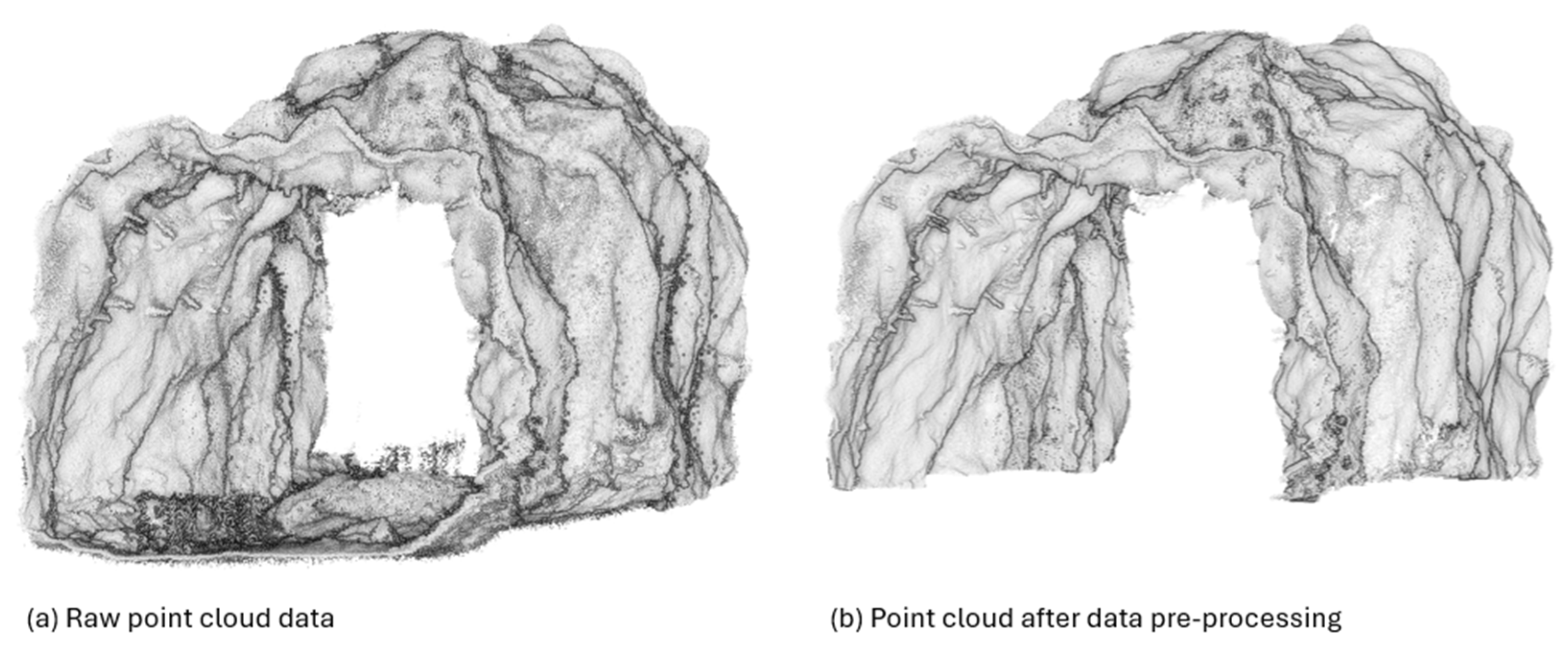
The k-nearest neighbours (k-NN) filter is employed in this study to remove isolated erroneous points based on the spatial relationship between each point and its surrounding neighbours. Such noise in the point cloud often arises due to sensor perturbations and laser beam divergence, which can introduce inaccuracies in the range measurements captured by the laser scanner. The algorithm evaluates the local geometry by fitting a plane through the nearest points and identifies outliers based on deviations from this plane. However, selecting an excessively large number of neighbours increases the algorithm’s sensitivity to the fitted surface, potentially eliminating valid inlier points and reducing point cloud density. Since plane fitting requires at least four non-collinear points, the number of neighbours must be carefully chosen. Through trial-and-error, it was observed that setting this parameter beyond 15 significantly degraded the dataset. Therefore, the number of neighbours was constrained between 4 and 15, with an optimal value of 6 used in this study.
The cloth simulation filter (CSF) is applied to remove the floor from the scans, which is irrelevant to rock bolt detection. CSF operates by inverting the point cloud and simulating a cloth that is gradually lowered onto the surface under gravity-like forces. As the cloth conforms to the geometry, it separates lower-lying regions from elevated features. The cloth is represented as a grid of interconnected nodes, and its flexibility and resolution are controlled by parameters. In this study, the node spacing of the cloth (grid distance) was set between 25 and 100 times the average point spacing, ensuring an appropriate balance between resolution and computational efficiency. The number of iterations was set between 400 and 500, in line with the previous literature suggesting the range was sufficient to achieve stable and accurate terrain simulation. Additionally, a threshold distance of 0.5 m from the simulated terrain, empirically derived through trial-and-error, was used to classify and remove floor points, including fragmented rocks and debris commonly found near the base of the scans. This approach effectively segregates the structural surfaces of interest from the ground points.
As a final pre-processing step, connected component filtering is applied to remove isolated sets of points that are disconnected from the main segment of the scanned data. These points often appear as random, isolated sections in the point cloud, resulting from false range measurements, stray objects captured in the scan that are not part of the mine surface, dynamic objects obscured during scanning, or rock debris that passes through the CSF and remains in the floor region. The connected component filtering works by grouping points that are spatially connected based on a defined neighbourhood relationship, typically using an octree structure to efficiently manage spatial data. In this study, an 11th-level octree with a grid size of 0.016 m was used. The choice of an 11th-level octree balances resolution and computational efficiency, maintaining adequate detail without significantly increasing processing time. A minimum threshold of 10,000 points per component was set to ensure that only significant, spatially coherent regions are segmented. Components with fewer points than this threshold are discarded.
These methods are selected over other filtering algorithms as they are standard survey point cloud pre-processing steps [
10] that effectively remove noise and erroneous points while preserving the integrity of the remaining data and requiring relatively low processing time [
15,
27]. Importantly, all rock bolts were preserved during pre-processing, and no bolt was unintentionally removed. Only spurious points surrounding the bolts, considered as noise, were removed to enhance the definition of the bolts. A comparison between the raw and pre-processed point cloud example scan is illustrated in
Figure 2.
2.4. Deep Learning Model for Rock Bolt Identification
One of the key advantages of deep learning-based point cloud semantic segmentation models is their ability to automatically learn feature representations for classifying points, eliminating the need for manual feature definition [
28,
29]. Traditional machine learning algorithms, in contrast, require predefined features, which is challenging because it is difficult to determine which features are most relevant for distinguishing between classes [
30]. Additionally, manually defining features increases processing complexity, as models must operate on a point cloud plus per-point large feature vectors, rather than a simpler point cloud vector, leading to significantly longer processing times.
Despite these advantages, using deep learning to identify rock bolts in complex MLS point clouds of underground mines presents a major challenge due to severe data imbalance. Rock bolts are extremely small objects in large-scale underground point clouds, with non-bolt points (class 0) outnumbering bolt points (class 1) by approximately 100:1 in the pre-processed scans. This imbalance makes it difficult for standard deep learning models to learn meaningful representations for rock bolts. To address these challenges, this paper proposes
DeepBolt, a novel deep learning architecture designed for automatic rock bolt identification in complex 3D point clouds captured using MLS.
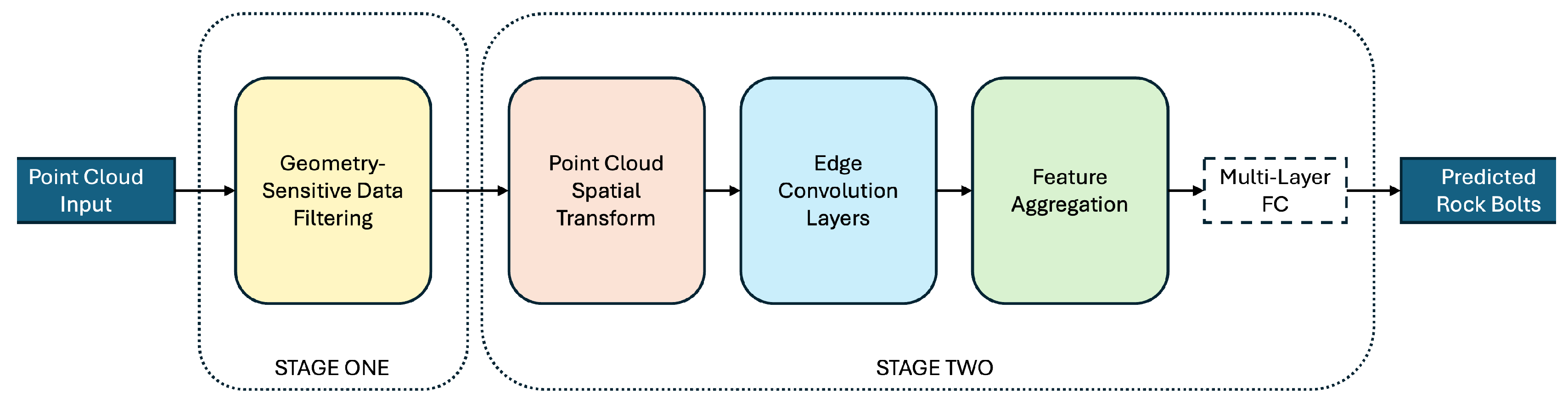
DeepBolt follows a two-stage approach (
Figure 3). In the first stage, it mitigates the data imbalance by filtering out redundant non-bolt points from the environment, increasing the relative proportion of bolt points in the dataset. In the second stage, a graph-based deep learning model, inspired by a dynamic graph convolutional neural network [
31], performs semantic segmentation to accurately extract rock bolts from the point cloud. This two-stage design enhances both efficiency and accuracy, making
DeepBolt well-suited for rock bolt detection in challenging underground environments.
2.4.1. Stage One—Geometry-Sensitive Data Filtering
Within the point clouds of underground mines, rock bolts are narrowly perceptible due to their extremely small size, resulting in a significant class imbalance when attempting to identify them. Therefore, a filtering strategy is required to selectively remove unwanted background and non-bolt points without impacting the actual rock bolt points. This would increase the ratio of bolt points to non-bolt points, thereby reducing the data imbalance. To achieve this, a strategy is needed that can roughly differentiate between rock bolts and the surrounding environment. Widely used filtering methods such as uniform voxel downsampling, moving least squares filtering, and region growing filtering are unsuitable for this application, as they cannot distinguish between rock bolts and the environment, leading to similar results across the entire point cloud. In contrast, the geometry-sensitive filtering strategy leverages the cylindrical nature of the visible protrusion sections of rock bolts, which distinguishes them from surrounding elements in the environment. By focusing on this geometric characteristic, the proposed filtering strategy effectively retains rock bolt points while reducing irrelevant background non-bolt points, thereby mitigating the severe class imbalance present in the data.
To understand the geometric characteristics of a surface based on how points are distributed within a local neighbourhood, Principal Component Analysis (PCA) is applied to the point cloud to compute three eigenvalues
λ1,
λ2,
λ3. PCA decomposes the local covariance matrix within a defined support region around each query point, producing three eigenvalues that quantify the variance along the three principal axes [
32,
33]. The optimal radius for this support region is strategically determined as
PS.(5–16. PS), where
PS represents the point spacing in metres. This formulation ensures that for lower point spacing, the weight multiplied to the point spacing is larger, while for higher point spacing, it is smaller, adapting dynamically to different scanning resolutions [
34]. In this study, with a point spacing of 0.008 m, the computed radius of influence is 0.039 m.
The three eigenvalues characterise the local surface structure, with
λ1 representing the primary direction of variance,
λ2 capturing secondary variations, and
λ3 corresponding to the least significant direction. Using these eigenvalues, key geometric features in geotechnical applications—planarity, omnivariance, and curvature—are derived for each point in the point cloud, as defined in Equation (1). These features provide critical insights into the local shape of a surface.
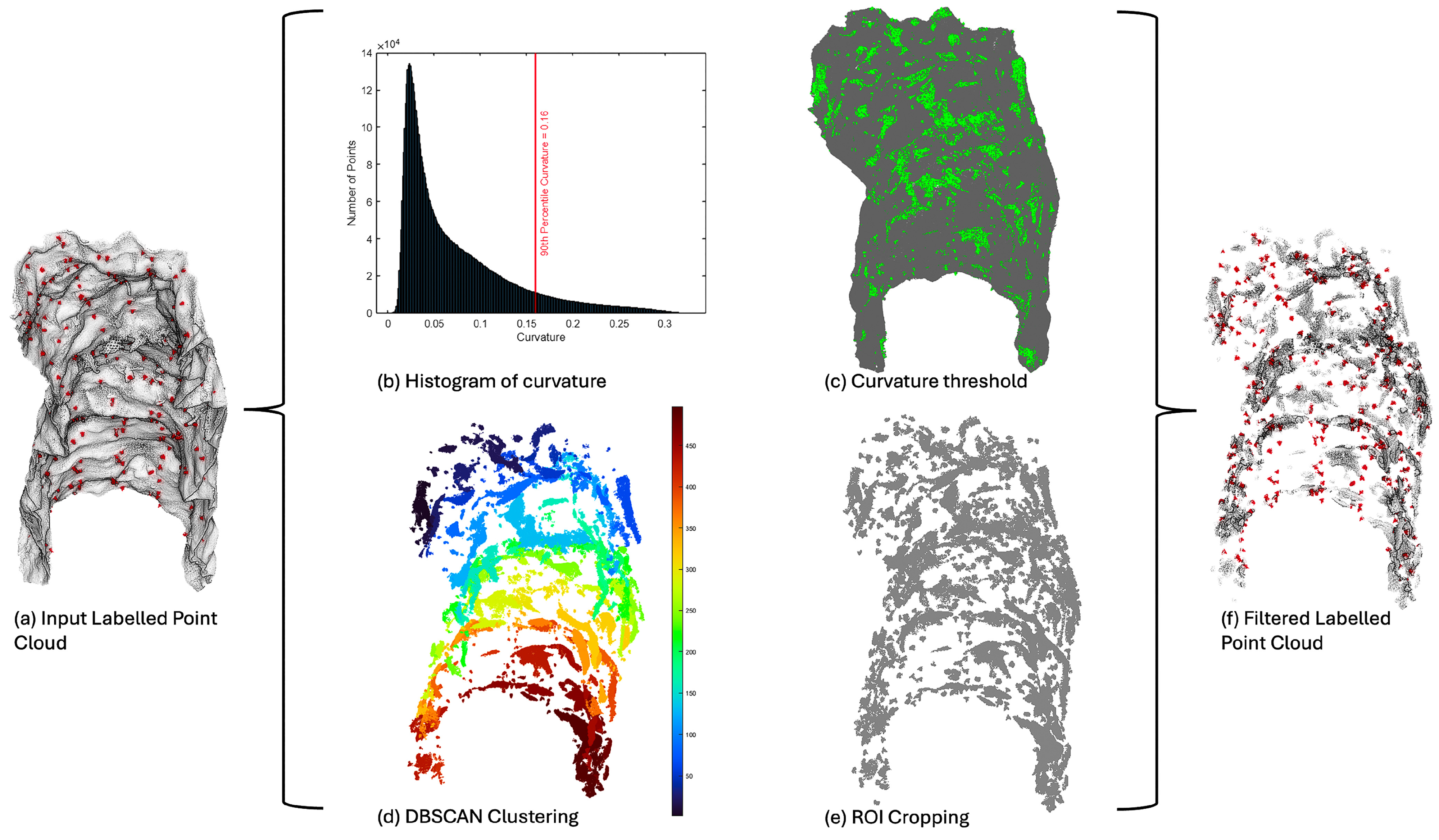
To analyse the effect of the three geometric features on the point cloud, the data are visualised in RGB space, with colours representing the varying degrees of each feature (
Figure 4). A detailed analysis of the three features are as follows:
Planarity measures how well a local neighbourhood of points aligns with a plane. As shown in
Figure 4a, planarity values are high for well-defined planar surfaces, such as discontinuity planes, and low for non-planar regions, such as edges and bolts. However, while planarity effectively highlights flat surfaces, it is less effective for distinguishing low-planarity regions like rock bolts from other non-planar features, such as discontinuity edges, which also exhibit low planarity.
Omnivariance quantifies the isotropy of the point distribution, capturing how evenly variance is spread across all three principal directions. In
Figure 4b, omnivariance values are high for bolts but also remain high in certain discontinuity plane regions, reducing its effectiveness as a distinguishing feature for rock bolts.
Curvature measures the variation along the smallest principal direction, indicating how much a surface deviates from a plane. As seen in
Figure 4c, all rock bolts exhibit high curvature values, making curvature the most reliable feature for identifying bolts. Although some other regions such as hanging objects and uneven local surfaces also display moderately high curvature, further refinement in subsequent processing steps, including semantic segmentation, ensures the removal of such unwanted points. Most importantly, all bolts in the point cloud consistently exhibit high curvature, making it a key discriminative feature in the filtering process.
With curvature identified as the key geometric feature for distinguishing rock bolt regions, an appropriate threshold must be determined to separate regions of interest from background points. This is achieved by computing the 90th percentile of the cumulative distribution function (CDF) of curvature values. Based on empirical observations, it was found that the 92nd percentile is the upper limit for ensuring 100% of the bolts are preserved, as all bolts exhibit curvature values above this mark. Thresholds below the 92nd percentile still maintain 100% bolt preservation; however, they begin to increase the amount of background environment retained in the filtered data. Therefore, the 90th percentile threshold is empirically chosen, as it ensures complete bolt preservation while maintaining a buffer margin for reliability and reducing the inclusion of unwanted background information. A fixed curvature threshold is unsuitable due to variations across different datasets. Unlike mean- or median-based methods, which can be heavily influenced by the dominant background points and lead to overly conservative thresholds that fail to isolate the rare, high-curvature bolt regions, the percentile-based approach specifically targets the upper tail of the distribution where the bolts lie. Instead, this dynamic, percentile-based approach enhances automation while minimising potential errors. The selected 90th percentile value is visualised in the histogram of curvature of one of the scans (
Figure 5b), providing an intuitive representation of the threshold selection.
Once established, the threshold effectively separates the point cloud into two categories (
Figure 5c):
To further refine the selection and filtering process, density-based clustering (DBSCAN) is applied to the set of high-curvature points (
Figure 5d). DBSCAN identifies clusters based on spatial proximity, effectively grouping potential rock bolt regions while treating isolated points as noise and removing them. DBSCAN was chosen over other clustering methods because it does not require the number of clusters to be predefined, can identify clusters of arbitrary shape, and is highly robust in segregating noise from clusters in point cloud data. The choice of DBSCAN parameters is guided by key factors such as point density, rock bolt distribution, bolt size, and the average number of points per bolt. The maximum neighbourhood distance (ε) is set to 0.1 m, which is half of the maximum visible protrusion of a typical bolt (0.2 m) and significantly smaller than the spacing between adjacent bolts. This ensures that all points along a single bolt are grouped together without inadvertently clustering in points from neighbouring bolts. The minimum cluster size is set to 50 points, which is half the number of points typically observed in the smallest bolts within the dataset (approximately 100 points). This provides a buffer to accommodate partially visible bolts in the filtered data while maintaining robustness against noise by preventing the formation of clusters from sparse, irrelevant noise points.
To finalise the regions of interest (ROI) as seen in
Figure 5e, each high-curvature cluster identified by DBSCAN is evaluated based on two conditions. A rough threshold,
Gth is set to 400, as no individual rock bolt in the dataset exceeded this size.
Clusters larger than Gth are directly added to the final filtered point cloud. These clusters are likely to represent localised high-curvature regions that may or may not contain bolts. Retaining them ensures that any bolts within these regions are not inadvertently discarded.
Clusters smaller than or equal to Gth are refined further. A region of interest (ROI) is defined around the cluster centroid, and all points within a 0.1 m search radius are extracted and added to the filtered point cloud. This step compensates for cases where some portions of a bolt may have been removed from the high curvature set because of exhibiting lower curvature due to local noise, thereby ensuring that entire bolts are preserved. The 0.1 m radius is chosen strategically, as the maximum visible protrusion of a bolt is approximately 0.2 m; thus, a 0.1 m radius around the cluster centroid can effectively capture the full extent of the bolt in all directions while minimising excessive inclusion of extraneous data.
A comprehensive overview of the geometry-sensitive data filtering strategy is presented in
Figure 5. The approach effectively mitigates class imbalance, as evident in the filtered, labelled point cloud (
Figure 5f). A substantial portion of background points has been successfully removed while preserving rock bolt points, thereby increasing the ratio of bolt points to non-bolt points. Additionally, the reduction in background points also optimises computational efficiency; fewer points result in faster processing, thereby improving the training and testing times for subsequent semantic segmentation tasks. However, despite the substantial reduction in background points, some amount of non-bolt high-curvature regions persist after the filtering step. These residual points are subsequently addressed through the deep learning-based segmentation model in
Section 2.4.2. A detailed pseudocode of the geometry-sensitive data filtering strategy can be seen in Algorithm 1.
| Algorithm 1 Geometry Sensitive Data Filtering |
| | Input: point cloud P of an underground mine |
| | Output: filtered point cloud Pfiltered with reduced class imbalance |
| 1 | Compute average point spacing PS using mean distance of points with nearest neighbour |
| 2 | Compute radius of influence r ← 5*PS–16*PS2 |
| 3 | for each point pi ∈ P do |
| | | Find neighbouring points of pi in spherical support region of radius r |
| | | Extract and store eigenvalues λ1, λ2, λ3 ← PCA(pi) |
| | end for |
| 4 | Compute geometric curvature measure for all points C ← λ3./(λ1 + λ2 + λ3) |
| 5 | Compute the cumulative distribution function CDF of C |
| 6 | Determine the 90th percentile value Cth from the CDF |
| 7 | Classify points based on Cth: |
| | High-curvature points Ph ← {pi|Ci > Cth} |
| | Low-curvature points Pl ← P\Ph |
| 8 | Compute clusters G ← DBSCAN(Ph) |
| 9 | for each cluster gi ∈ G do |
| | | if cluster size |gi| > Gth then
Pfiltered ← Pfiltered + gi
else:
Compute centroid μi ← mean(gi)
Compute region of interest P’ ← points in P within radius 0.1 to μi
Pfiltered ← Pfiltered + P’ |
| | | end if |
| | end for |
| 10 | return Pfiltered |
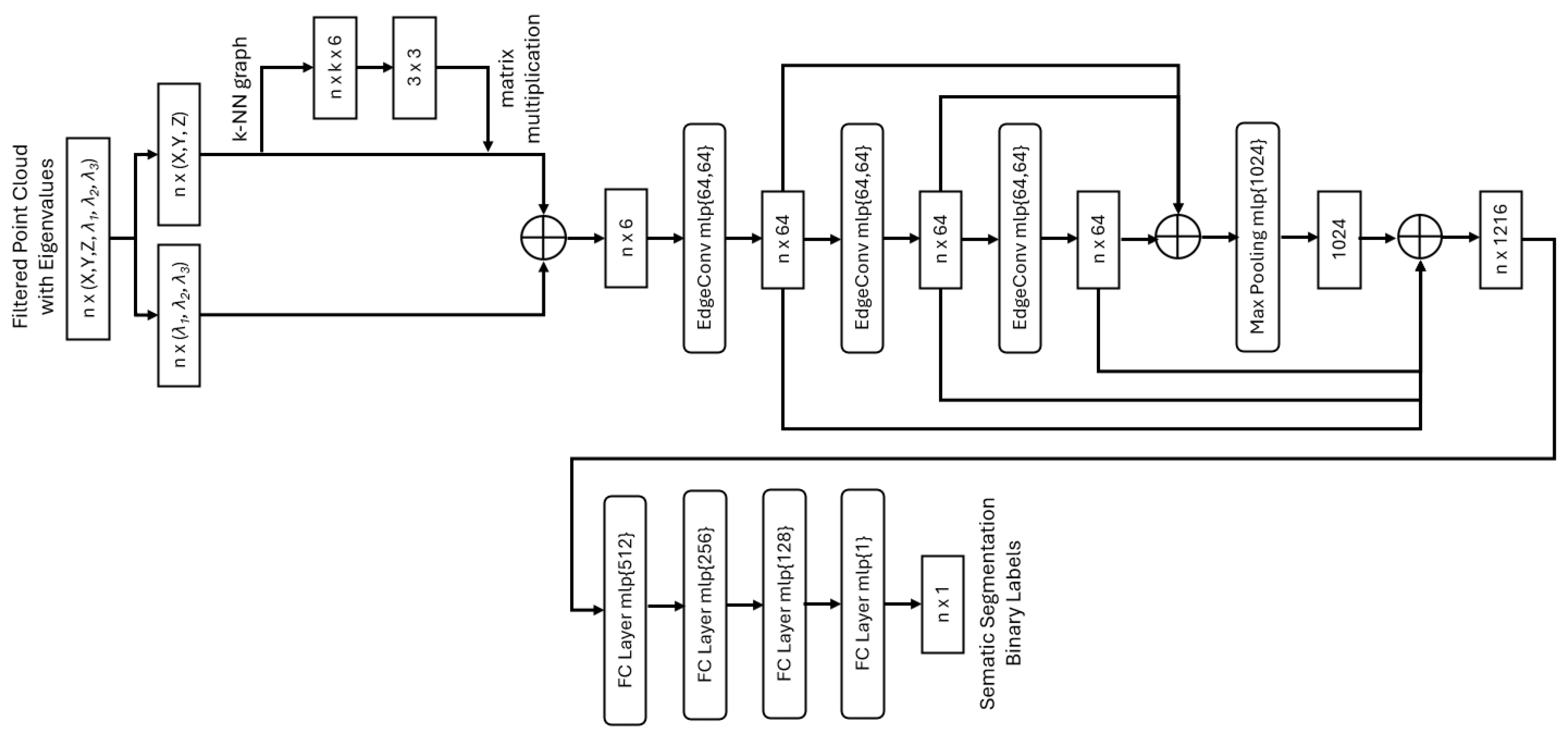
2.4.2. Stage Two—Semantic Segmentation
After applying the filtering process described in
Section 2.4.1, the resulting point cloud has significantly reduced background environment (class 0) while enhancing the representation of rock bolts (class 1). This filtering step provides a rough estimation, substantially improving the class imbalance between bolts and non-bolts from approximately 1:100 to 1:15. Achieving this improved balance is critical, as it prevents the segmentation model from being overwhelmed by the dominant non-bolt class, allowing it to better learn and distinguish features associated with rock bolts. This ultimately leads to greater segmentation accuracy, stability, and faster convergence during training.
The next stage involves using semantic segmentation to accurately identify rock bolt protrusions within the filtered point cloud, ultimately isolating the final rock bolts. To achieve this, a graph-based semantic segmentation model inspired by the deep learning model, the dynamic graph convolutional neural network (DGCNN), is used in this study. The complete architecture of our model can be seen in
Figure 6. Unlike conventional models that rely on CNNs and MLPs, which often struggle to capture the inherent local geometric structures in point clouds [
35,
36], our graph-based approach overcomes this limitation by dynamically constructing local neighbourhoods in feature space rather than using fixed receptive fields. By dynamically reconstructing local neighbourhoods in the evolving feature space at each layer, rather than relying on fixed neighbourhoods as in static graph models, the network can better adapt to variations in local geometry and complex structures, and improve feature discrimination between bolts and background. This flexibility enables a more robust feature representation, preserving spatial relationships, adapting to varying point densities, and effectively capturing geometric structures. As a result, the model can accurately distinguish rock bolts from complex backgrounds. The key components of
DeepBolt’s semantic segmentation model that transform the input into per-point class labels are as follows:
Input Layer: The model takes as input an
n × 6 matrix, where
n is the total number of points in the filtered point cloud. Each row consists of the spatial coordinates (
X,
Y,
Z) and the eigenvalues (
λ1,
λ2,
λ3) computed in
Section 2.4.1. Incorporating eigenvalues alongside point coordinates enhances the geometric representation of the data, allowing the model to better capture local structural variations. This additional geometric context also accelerates model convergence, as eigenvalues have already been shown to be crucial in characterising the geometric properties of a point within its neighbourhood.
Point Cloud Spatial Transform Block: The point cloud transform block aligns the input point set to a canonical space by estimating and applying a 3 × 3 transformation matrix, ensuring invariance to rotations and translations. To compute this matrix, a tensor is formed by concatenating each point’s coordinates with the coordinate differences between the point and its k = 20 nearest neighbours in the k-NN graph. This enriched representation captures both absolute positions and local geometric relationships, allowing the network to learn a transformation that enhances feature consistency for further processing.
Edge Convolution Layers (EdgeConv): After spatial alignment, the model applies a sequence of three EdgeConv layers, which operate on dynamically computed k-NN graphs (k = 20). Each EdgeConv layer updates the neighbourhood graph at every iteration, enabling the network to capture both local geometric relationships and long-range spatial dependencies. The edge features are processed through a multi-layer perceptron (MLP), which learns non-linear transformations to extract high-level representations from the local neighbourhood. By stacking multiple EdgeConv layers with MLPs, the network progressively refines feature representations.
Feature Aggregation: As the network progresses, multiple EdgeConv layers extract hierarchical features at different levels. Early layers focus on local details, while deeper layers capture global contextual information. The extracted features from different layers are concatenated to preserve both fine and coarse details, ensuring a robust segmentation of rock bolts even in complex underground environments.
Fully Connected Layers: Finally, the model applies fully connected layers to predict per-point class labels. A combination of local and global features is processed through an MLP, which outputs class logits for each point. Instead of softmax, a sigmoid activation function is used, as it produces a single probability for the positive class (rock bolt). The choice of sigmoid over softmax is driven by the binary nature of the classification task, where the model only needs to distinguish between two classes: rock bolt and non-bolt. This simplifies the model, reducing complexity by requiring just one output neuron instead of a neuron for each class, as would be the case with softmax. Sigmoid activation is computationally more efficient, requiring only a single neuron for binary class, and facilitates handling class imbalance through weighted loss functions. Additionally, it avoids unnecessary competition between outputs, resulting in more stable gradients. This activation function enables the final binary segmentation output. By leveraging graph-based dynamic feature extraction, the network ensures accurate segmentation of rock bolts, even in noisy, high-clutter environments.
To effectively train the model and refine its segmentation accuracy, the model employs a weighted sigmoid binary cross-entropy loss function. This approach outperforms other loss functions in scenarios involving class imbalance, such as the detection of rock bolts in point cloud data, by addressing the unequal distribution of the target classes. Given that rock bolt points are outnumbered by background points in the input to the model at a ratio of approximately 1:15, the loss function is adjusted to assign a higher penalty to misclassifications of the minority rock bolt class. This weighting ensures that the model learns to correctly identify rock bolts despite their lower representation in the dataset. Accordingly, the loss function applies weights of 15/16 to rock bolt points and 1/16 to background points using a normalised inverse frequency scheme. The mathematical formulation of the loss function used in the model is presented in Equation (2).
where
σ(x) is (sigmoid function);
y ∈ {0, 1} (true label);
x is logits before sigmoid activation;
w+ is 15/16 (weight for rock bolt class);
w− is 1/16 (weight for non-bolt class).
As outlined in
Section 2.2, the dataset comprises a total of 1764 rock bolts. To prevent overfitting, the dataset was split into two parts such that filtered point cloud scans consisting of 1468 bolts were used for training, while the remaining scan with 296 bolts was reserved for testing. A 10-fold cross-validation approach was employed during the training process, where each fold consists of nine subsets used for training and one unique subset for validation. To monitor the stability and convergence of the training, both training and validation loss curves were tracked over 100 epochs. As shown in the learning curve (
Figure 7), the training loss exhibits a consistent decline, indicating effective learning, with early training phases showing higher fluctuations due to initial weight updates, but as training progresses, the loss stabilises, signalling convergence. Similarly, the validation loss follows a comparable trend, stabilising similarly to the training loss after several epochs. This parallel behaviour suggests that the model generalises well to unseen data, effectively learning the underlying patterns rather than memorising the training set. As a result, the model does not overfit, and the validation loss decreases steadily, reinforcing the model’s ability to predict unseen data. The model’s loss plateaus and converges after 32 epochs, establishing this as the optimal number of epochs for training. For optimising the loss function, the Adam optimiser was used with an initial learning rate of 0.001, momentum of 0.1, and a batch size of 16, with momentum decay set to 0.5 every 16 steps. The model was implemented using PyTorch v2.2.0 and takes approximately 8 h to converge in 32 epochs on an NVIDIA T1000 GPU (8GB VRAM, 896 CUDA cores).
2.5. Evaluation Metrics
To evaluate the semantic segmentation performance of
DeepBolt, it is compared against several deep learning models, including PointNet [
37], PointNet++ [
38], KPConv [
39], RandLA-Net [
40], and DGCNN [
31]. PointNet is a deep learning architecture for point cloud classification and segmentation that directly processes raw 3D points, capturing global geometric features. PointNet++ is an extension of the PointNet framework and captures local context by hierarchically aggregating features through a series of spatially grouped regions, improving performance on complex structures. KPConv introduces a kernel-based convolution approach for 3D point clouds that uses learnable convolution kernels, allowing for more flexible and efficient feature extraction on irregular point sets. RandLA-Net offers a lightweight, efficient deep learning model for large-scale 3D point cloud segmentation, utilising random sampling and local aggregation to achieve high accuracy with reduced computational cost. Lastly, DGCNN employs a dynamic graph convolutional network that models point cloud data through dynamic graph structures, enabling robust feature extraction by considering the relationships between points. These models are widely adopted state-of-the-art architectures for point cloud processing and have been extensively used as benchmarks in numerous 3D segmentation applications due to their robustness and efficiency [
41,
42,
43], thereby providing a baseline for comparative evaluation of our proposed model.
The semantic segmentation performance of these models is evaluated using the Intersection over Union (IoU) metric for both bolts and non-bolts. IoU measures the overlap between the predicted segmentation and the ground truth, indicating how well the model identifies each class. The formula for calculating IoU for a given class (bolt or non-bolt) is provided in Equation (3).
where
To assess the overall performance of the proposed
DeepBolt as a rock bolt identification technique, it is compared against two of the latest techniques in the literature, BoltANN [
13] and CanupoBolt [
15], as described in
Section 1. These techniques are specifically designed for rock bolt detection in underground coal mining environments, reflecting practical approaches tested on field data, and thereby serve as strong baselines to demonstrate
DeepBolt’s domain-specific improvements. The evaluation is based on standard classification metrics, precision, recall, and F1 score, as defined in Equation (4), using the test dataset containing 296 ground truth bolts. True positives (TP) refer to bolts correctly identified as such, false positives (FP) are incorrectly identified bolts that do not correspond to ground truth, and false negatives (FN) are actual bolts that were missed by the model. Precision measures the proportion of predicted bolts that are actually correct, recall measures the proportion of actual bolts that were successfully identified, and F1 score provides a balanced measure that considers both precision and recall.
3. Results and Discussions
This section provides a comprehensive analysis of the results obtained using the proposed method described in
Section 2. The experiments were conducted on a system with the following computational specifications: a 3.90 GHz Intel
® Xeon
® W-2245 64-bit processor, 128 GB of system memory, and an NVIDIA T1000 GPU with 8 GB VRAM and 896 CUDA cores.
3.1. Evaluation of Geometry-Sensitive Filtering Strategy
As established in
Section 2.4,
DeepBolt employs a geometry-sensitive filtering strategy to address the massive class imbalance present in the dataset. The effectiveness of this strategy was assessed using three key metrics: (i) the percentage of background points removed, (ii) the percentage of individual rock bolts preserved, and (iii) the average percentage of rock bolt points retained after filtering.
An example scan processed with the filtering strategy is illustrated in
Figure 8, highlighting key regions of interest. The visualisations include (a) an individual bolt within the region of interest, (b) a bolt located in a local high-curvature area, and (c) a high-curvature structure that is not a rock bolt but still passes through the filtering process. While large portions of background noise are removed, certain stray high-curvature objects persist. This is because the filtering is based on geometric features, which may not always uniquely identify all background elements from objects of interest. Additionally, the complexity of the rock mass environment, with varying shapes and curvatures, poses challenges in setting optimal thresholds that balance background removal with the retention of key features. These persistent stray background points are subsequently addressed by the semantic segmentation model. The primary goal of the filtering strategy is to reduce the class imbalance while ensuring that no critical bolt information is lost, thus limiting the degree of background removal. These visual results confirm the strategy’s ability to retain essential elements while minimising irrelevant background environment.
A quantitative evaluation of the filtering strategy is presented in
Table 3, summarising results from eight different scans. On average, 85% of background points were removed, while 98.37% of rock bolt points were preserved. The minor loss in bolt points can be attributed to edge cases where portions of bolts were excluded due to local high-curvature considerations or data noise. However, this minimal loss has a negligible impact on the final segmentation and intersection-over-union results since the overall loss is less than 2%. More importantly, 100% of individual rock bolts were retained in all cases, ensuring that no complete bolts were lost during the filtering process.
The variations observed in the percentage of background removal and bolt point preservation across different scans can be attributed to local scan factors such as variations in curvature, environmental structures, and data noise. Despite these variations, the method consistently achieves over 80% reduction in non-bolt points while preserving over 98% of bolt points, making it a robust and reliable approach for improving the representation of rock bolts in underground mine point clouds. As a result, the class imbalance between bolts and non-bolts is successfully reduced from approximately 1:100 to 1:15, significantly mitigating the severe class imbalance in the dataset for subsequent processing.
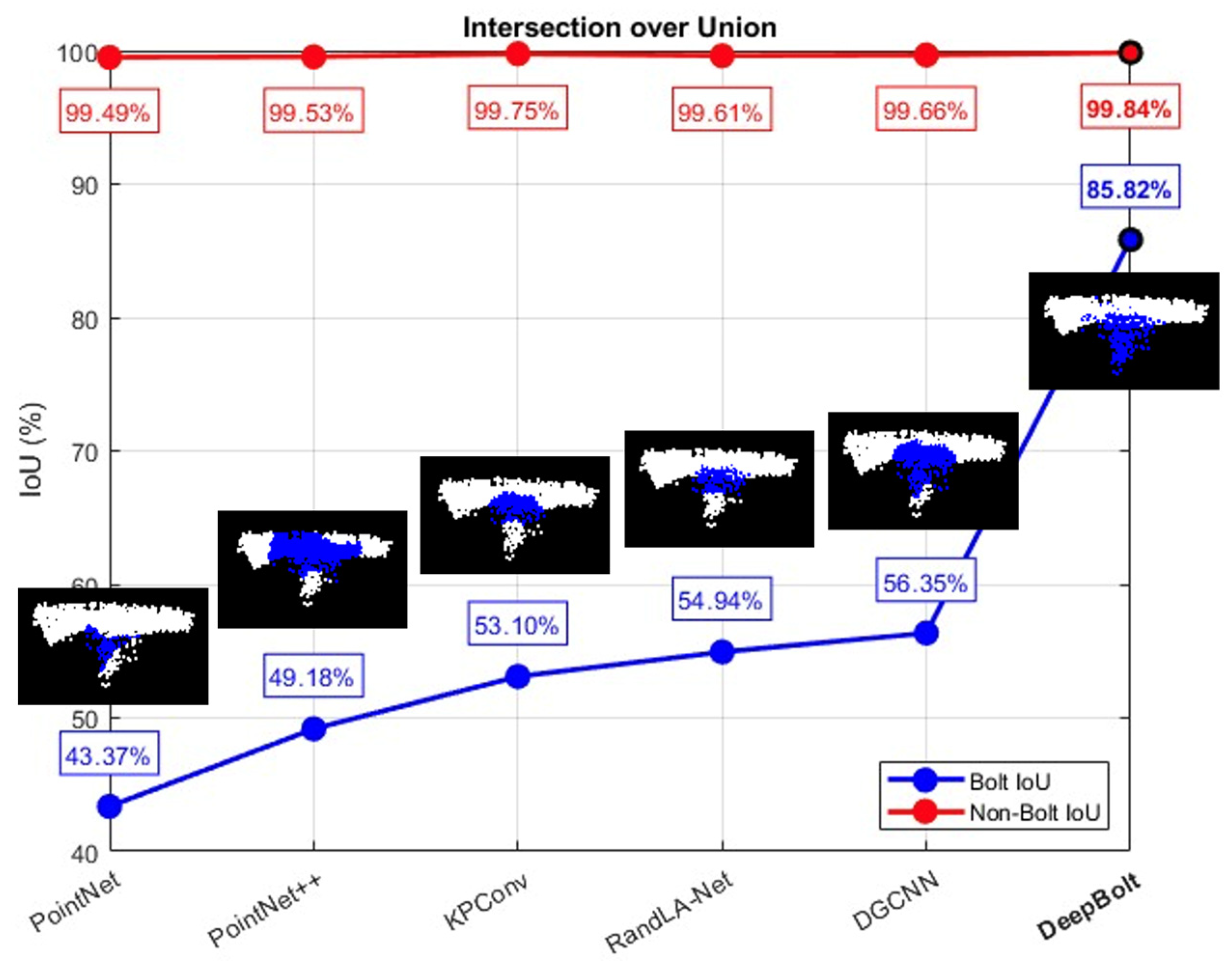
3.2. Evaluation of Semantic Segmentation and Overall Rock Bolt Identification Performance
The rock bolt semantic segmentation results of
DeepBolt, compared to other semantic segmentation models mentioned in
Section 2.5, are shown in
Figure 9. The observed performance differences between the compared models stem from variations in local feature aggregation, robustness to class imbalance, and adaptability to the complex spatial distributions typical of underground mine point clouds.
DeepBolt outperforms all other models in terms of both bolt and non-bolt IoUs. Specifically, it achieves a significant improvement in bolt IoU, with an increase ranging from 29.5% to 42.5%. This enhancement is attributed to the fact that existing models are not optimised to handle severe class imbalance or detect small objects like rock bolts in large-scale, complex point clouds of underground mines.
DeepBolt’s superiority in accurately segmenting bolts is also evident in the visualisation of an example candidate rock bolt, with segmentation results from different methods shown in
Figure 9. As is visible,
DeepBolt accurately delineates the boundary of the candidate bolt protrusion, whereas other methods either miss substantial regions or misclassify parts of the background. Unsurprisingly, the gain in non-bolt IoU is relatively modest, approximately 0.4%, since over 99% of the point cloud consists of background environment. Overall, the IoU results highlight
DeepBolt’s superior capability in accurately segmenting rock bolts in complex environments.
To isolate the contributions of the two stages in DeepBolt, an ablation study was conducted. This involved comparing the Intersection over Union (IoU) scores for bolt and non-bolt classes at different stages of the DeepBolt pipeline as follows:
Semantic segmentation model only: The resultant bolt IoU is 59.23% and non-bolt IoU is 99.85%.
Geometry-sensitive filtering + semantic segmentation model: The resultant bolt IoU is 85.82% and non-bolt IoU is 99.84%.
The results demonstrate that the addition of the geometry-sensitive filtering strategy leads to a substantial improvement in bolt IoU, an increase of 26.59%. This gain is attributed to the filtering step, which mitigates the severe class imbalance, thereby enabling the segmentation model to make more accurate predictions. The non-bolt IoU displays insignificant change, indicating that background classification performance is unaffected, in line with the trends observed in
Figure 9.
A detailed analysis of the rock bolt classification performance can be seen in
Table 4.
DeepBolt achieved the highest number of true positives while minimising both false positives and false negatives. It delivered an impressive precision of 94.41%, a recall of 96.96%, and an F1 score of 0.96, outperforming both BoltANN and CanupoBolt. While BoltANN and CanupoBolt showed comparable recall values, BoltANN had a slight edge in precision between the two. When compared to its counterparts,
DeepBolt improved upon BoltANN’s precision by 4.88% and CanupoBolt’s by 7.57%. In terms of recall, it surpassed BoltANN by 7.43% and CanupoBolt by 7.76%, while the F1 score showed an improvement of 0.06 over BoltANN and 0.08 over CanupoBolt. These results clearly demonstrate
DeepBolt’s superiority in accurately identifying rock bolts within complex 3D point clouds of underground mines, thereby validating the effectiveness of this deep learning-based approach. The lower false positives and false negatives in
DeepBolt significantly enhance the practical usability of
DeepBolt compared to BoltANN and CanupoBolt, ensuring fewer background misclassifications (higher precision) and fewer missed bolts (higher recall), both critical for reliable and real-world application of automated bolt identification.
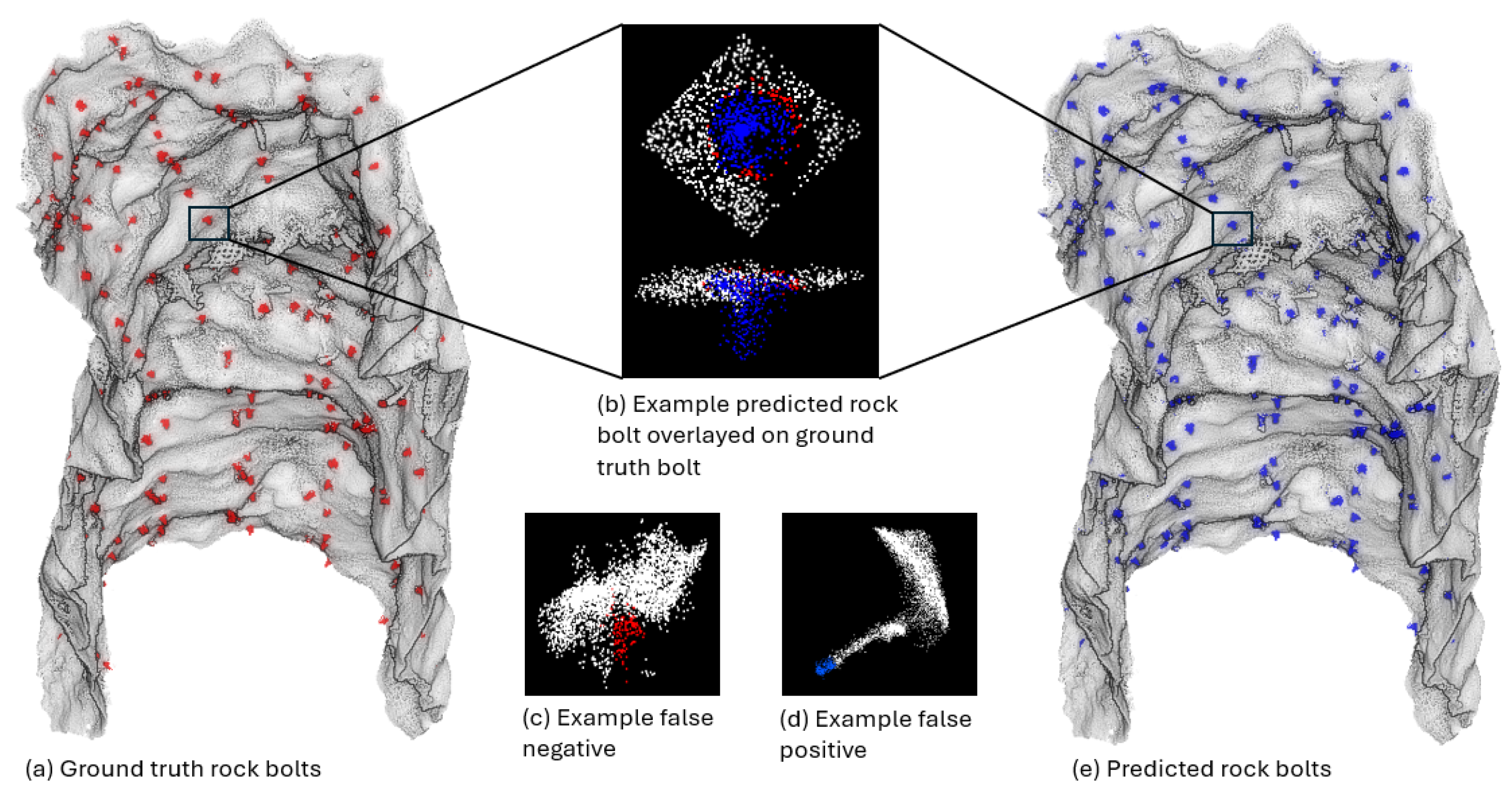
The semantic segmentation and the overall rock bolt identification performance of
DeepBolt can be visualised in
Figure 10. The ground truth rock bolts (
Figure 10a) and the predicted rock bolts (
Figure 10e) are marked in red and green, respectively, in the testing data. The figure includes an example where a predicted bolt is overlaid on the ground truth, clearly demonstrating the accuracy of the segmentation (
Figure 10c). The predicted bolt aligns closely with the ground truth, with only minor discrepancies observed near the base of the bolt. These small differences likely stem from slight variations in the manual labelling of the point cloud and minor inaccuracies in prediction. Importantly, there is no noticeable deviation in the prominent cylindrical section of the bolt. This visual comparison highlights
DeepBolt’s strong performance and its ability to accurately identify rock bolts in complex 3D environments.
The overall precision and recall of
DeepBolt are reduced by the limited number of false negatives (
Figure 10c) and false positives (
Figure 10d) present in the data, which can be attributed to specific challenges inherent to the nature of the point cloud in underground mining environments. False positives primarily arise from complex background geometries that locally resemble bolts in shape and size, such as loose wire cables, pipes, sensor noise-induced artefacts or other cylindrical bolt-like structures. Despite the model optimisations, some of these structures exhibit similar local features to actual bolts, leading to occasional misclassification. On the other hand, false negatives are mainly caused due to occlusions, point scarcity, partial scanning of bolts, or bolts embedded within highly irregular or fractured surfaces, where distinctive geometric features are insufficiently captured or distorted, making rock bolt identification in such areas challenging for the model. A further reason for error is the presence of minor inconsistencies or noise in the training sample, often arising from biases in manual annotation. These imperfections can introduce subtle interclass overlaps during training. Despite these minor errors,
DeepBolt demonstrates significantly higher accuracy than existing models, highlighting its robustness. Future improvements could involve incorporating additional semantic features, such as intensity, to enhance interclass separability, along with the use of advanced, context-aware post-processing techniques to further reduce misclassification.
3.3. Execution Times
The average computation time for identifying rock bolts in a test scan using
DeepBolt is summarised in
Table 5. The table outlines the execution times for each step in the pipeline, excluding the time required to train the semantic segmentation model. Model training takes approximately 8 hours to converge over 32 epochs. While the geometry-sensitive filtering strategy incurs a relatively high computational cost, it plays a critical role in addressing the severe class imbalance by significantly reducing background points. This reduction improves the efficiency and accuracy of the subsequent semantic segmentation step. The entire process of identifying rock bolts in a test scan covering ~45 m of real-world underground mine section takes approximately 1650 s in total. The execution times are limited by the computational resources used for this study and can be further optimised by using upgraded overall hardware, including faster processors, GPUs with more cores and higher memory bandwidth, and improved storage systems to accelerate data handling and parallel processing.
A comparative analysis of
DeepBolt against other deep learning models and traditional rock bolt identification techniques based on model parameter counts and computational execution times is presented in
Table 6.
DeepBolt’s total computational complexity lies in the mid-range among the deep learning models. Although its total execution time is increased due to the geometry-sensitive filtering strategy, as seen in
Table 5, this step significantly reduces the input data size. As a result,
DeepBolt achieves the fastest semantic segmentation time among the deep learning models and even benefits from significantly shorter model training time. Among the traditional methods, BoltANN has the longest execution time, primarily due to its construction of a 58-dimensional feature space. In contrast, CanupoBolt performs faster, being a lightweight classifier based on a three-scale point descriptor. Since rock bolt identification is typically a post-processing step rather than a real-time task, accuracy holds greater importance than speed. While
DeepBolt is not the fastest approach, it outperforms all other deep learning and traditional techniques in terms of accuracy.
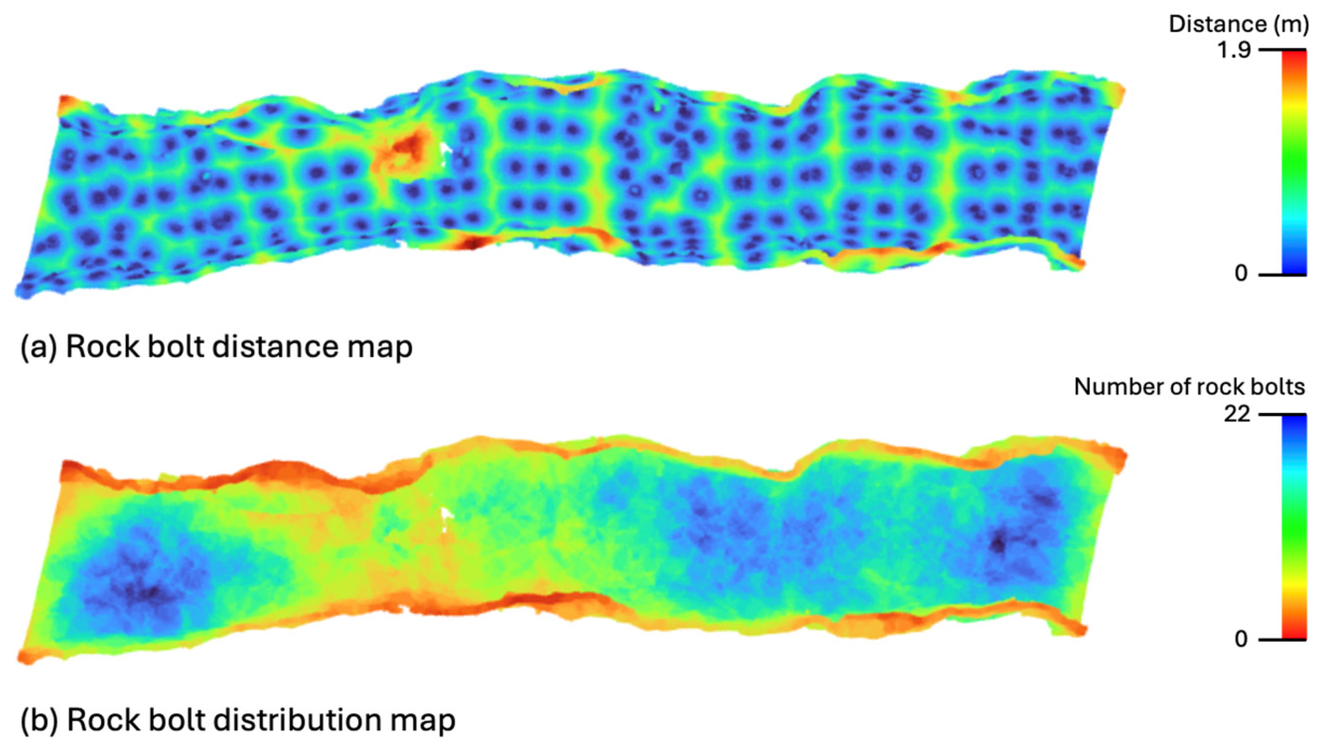
3.4. Rock Bolt Distance and Distribution Maps
Once rock bolts are accurately identified in the point cloud of underground mine sections, their spatial locations can be utilised to analyse the overall distribution and density of rock bolts across the scanned area. Using the identified bolt positions, two key visualisations are generated: the rock bolt distance map and the rock bolt distribution map, as shown in
Figure 11. The distance map (
Figure 11a) reflects how far each point in the point cloud is from the nearest bolt. Blue regions indicate close proximity (less than 0.6 m), while red areas represent points farther than 1.4 m from any identified bolt. Complementing this, the distribution map (
Figure 11b) conveys the density of bolts around each point by indicating how many bolts are found within a unit radius (set to 2 metres in this study). In this map, blue denotes areas with high bolt concentration (more than 16 bolts nearby), and red signifies sparse coverage (fewer than 6 bolts).
The accurate and automatic identification of rock bolts enables precise localisation of bolt positions within point clouds of underground mine sections. This capability forms the foundation for generating rock bolt distance and distribution maps, which together provide a comprehensive visualisation of the installed rock bolt support system. These maps are invaluable in informing key mining decisions: they help engineers and mine operators assess whether the existing bolt layout aligns with the intended support design, ensuring that support systems are in place where needed. Distance and distribution maps specifically assist in identifying areas requiring additional reinforcement, enabling efficient re-bolting operations, and ensuring that maintenance efforts are targeted where bolt presence is insufficient or deteriorated. By comparing actual bolt placements with mine support installation plans, these maps can reveal deviations from the original design, pinpointing areas of under-support or potential failures. Moreover, distribution and density maps can highlight changes in bolt presence over time, such as regions where bolts may have been dislodged, degraded, or lost, particularly in older mine sections. This capability is crucial for proactive maintenance and for identifying risk areas before they lead to safety concerns. With an automated approach like DeepBolt, using mobile laser scanning, such monitoring becomes not only more efficient and scalable but also significantly less labour-intensive compared to traditional manual inspections. As a result, the rock bolt identification technique offered by DeepBolt provides a practical, time-saving solution that greatly enhances the safety and integrity of underground mine environments by ensuring continuous and accurate monitoring of the rock bolt support system.
4. Conclusions
Rock bolts play a vital role in ensuring the structural integrity of underground mines by reinforcing weak rock strata and preventing hazardous events such as rockfalls. However, the challenging nature of manual rock bolt assessment necessitates an automated and scalable alternative. This paper presented a novel deep learning approach DeepBolt, for the automatic identification of rock bolts in complex, medium-to-large-scale 3D point clouds captured using SLAM-based mobile laser scanners in real-world underground mining environments. DeepBolt addresses several critical challenges in this domain, including severe class imbalance, high environmental variability, and the partial visibility of rock bolts due to face-plate obscurity caused by shotcrete application. It employs a two-stage approach combining geometry-sensitive filtering with a graph-based semantic segmentation network, specifically optimised for detecting small rock bolt objects in large-scale point clouds. Evaluation results demonstrated that our proposed architecture outperforms both state-of-the-art deep learning semantic segmentation models and current rock bolt identification techniques. The proposed method offers a robust, efficient, and scalable solution for automated rock bolt identification, enabling more frequent and reliable assessments of mine support systems. Future work can extend the DeepBolt training across different mine settings, geological conditions, and complex rock formations for further broadening the system’s generalisability and applicability. Additionally, this framework can also be extended to real-time bolt monitoring, predictive analytics of bolt conditions, multi-temporal analysis, or integration with digital twin environments to further enhance underground mine safety and operational efficiency.


