Channel Amplitude and Phase Error Estimation of Fully Polarimetric Airborne SAR with 0.1 m Resolution

Abstract

In order to achieve 0.1 m resolution and fully polarimetric observation capabilities for airborne SAR systems, the adoption of stepped-frequency modulation waveform combined with the polarization time-division transmit/receive (T/R) technique proves to be an effective technical approach. Considering the issue of range resolution degradation and paired echoes caused by multichannel amplitude–phase mismatch in fully polarimetric airborne SAR with 0.1 m resolution, an amplitude–phase error estimation algorithm based on echo data is proposed in this paper. Firstly, the subband amplitude spectrum correction curve is obtained by the statistical average of the subband amplitude spectrum. Secondly, the paired-echo broadening function is obtained by selecting high-quality sample points after single-band imaging and the nonlinear phase error within the subbands is estimated via Sinusoidal Frequency Modulation Fourier Transform (SMFT). Thirdly, based on the minimum entropy criterion of the synthesized compressed pulse image, residual linear phase errors between subbands are quickly acquired. Finally, two-dimensional cross-correlation of the image slice is utilized to estimate the positional deviation between polarization channels. This method only requires high-quality data samples from the echo data, then rapidly estimates both intra-band and inter-band amplitude/phase errors by using SMFT and the minimum entropy criterion, respectively, with the characteristics of low computational complexity and fast convergence speed. The effectiveness of this method is verified by the imaging results of the experimental data.

1. Introduction

High resolution and full polarization are two important research directions in the development of airborne SAR technology. The former aims to obtain higher-resolution ground target information by increasing the bandwidth of the transmission and reception signals [1,2,3,4,5], while the latter intends to acquire full-polarization feature information of ground targets by designing full-polarization signal transmission and reception channels [6,7,8,9]. To reduce hardware overhead and overall power consumption, the method of transmitting and receiving multiple-step-frequency modulation waveforms in a frequency-dividing manner is generally adopted, and range resolution can be improved through frequency-band synthesis. By transmitting and receiving fully polarimetric channel signals in a time-division manner, fully polarimetric imaging can be achieved. The combination of high-resolution and fully polarimetric technology can obtain more detailed and fully polarimetric features of ground targets, which is a typical application case of multidimensional SAR imaging. This technology has broad application prospects in geological exploration, military reconnaissance, forest census, agricultural remote sensing, land surveying and other fields [10].

The fully polarimetric airborne SAR system with 0.1 m resolution studied in this paper adopts frequency division technology in the frequency dimension, which utilizes step-frequency chirps and frequency band synthesis technology to achieve a high-range resolution. Moreover, time-division technology in the polarization dimension is applied to collect signals from different polarization channels by switching electronic switches.

Although this scheme can effectively reduce the hardware design difficulty caused by single-channel high-speed sampling, it also brings a series of problems. Due to the nonlinear characteristics of the power amplifier components, deviations in the phase-frequency characteristics of the subband signals from their ideal parameters are likely to occur. These deviations result in range defocusing, sidelobe asymmetry, paired echoes, and other anomalies of the subband image [11]. Furthermore, because distinct hardware paths are employed for signal transmission and reception channels, there is a significant deviation between the amplitude and phase characteristics of different channels and the ideal characteristics. Direct frequency band synthesis not only fails to improve the range resolution, but also causes severe image degradation. Additionally, there is a positional deviation between the images of different polarization channels. Consequently, the resulting image after polarization synthesis will have serious pixel mismatches, which cannot achieve the effect of high-resolution and full-polarization imaging. Therefore, accurate estimation of amplitude and phase errors in different frequency bands and polarization channels is a key issue that must be addressed in high-resolution and fully polarimetric airborne SAR systems.

Yi et al. proposed a Terahertz FMCW on-chip radar in 65 nm CMOS with an impressive 100 GHz bandwidth by means of frequency-comb architecture [3,4]. By skillfully designing five on-chip antennas and transceiver units on the CMOS chip, this on-chip radar had achieved a range resolution of 1.5 mm, which is creative and novel. Although it can achieve phase error correction for subband synthesis, the method cannot be directly applied to radar system with complex representations of the frequency-domain phase error and cannot solve the problem of paired echoes.

Deng et al. proposed a channel amplitude and phase correction method based on a spaceborne InSAR system [6], which adopts a redundant-channel scheme to collect internal and external calibration signals in real time. Although this scheme has been successfully applied, it suffers from high system hardware cost and method complexity.

Long et al. proposed a modified analysis of antenna vibration on GEO SAR imaging, which has an obviously curved trajectory, a high-order azimuth spectrum, and two-dimensional time-variant antenna gain [11]. Although a high-order ideal echo signal model and ideal point spread function of GEO SAR are established based on the curved trajectory, the method for paired-echo suppression cannot be directly applied to estimate amplitude and phase error for the high-resolution imaging of airborne SAR.

Liang et al. proposed a nonparametric paired-echo suppression method for helicopter-borne SAR imaging [12]. By constructing a modified vibration error model and introducing the autofocus method for the vibration phase error estimation, it can suppress the paired echoes directly, which avoids the complex vibration parameter estimation in the traditional methods. But the frequency and amplitude of real helicopter vibration error change randomly with time, and this method is not suitable for both the estimation of nonlinear and linear phase error within the subband spectrum.

Liang et al. proposed a polarimetric calibration scheme combining internal and external calibrations to calibrate the two types of polarization distortions for SAR with phased array antennas [13]. Although the scheme no longer depends on the distributed target and improves the polarization precision of the data, calibration equipment is required to solve for the parameters for constant polarization distortion, which is expensive and difficult for airborne SAR system.

Jung et al. presented a novel internal calibration system using a learning algorithm with gradient descent for the Ku-band radar system [14]. Aiming at reducing thermal drift caused by active components, internal calibration paths are designed to monitor gain deviations in HPA and LNA via a learning algorithm. This method can’t accurately measure amplitude and phase error caused by external loop, moreover extra hardware and computing resources are required, which is not suitable for the design of multi-band and fully polarimetric SAR system.

Wang et al. proposed a platform vibration parameter estimation algorithm based on DFrFT [15,16,17], which can estimate instantaneous vibration acceleration and frequency. Nevertheless, the accuracy of this algorithm depends on the length of the sliding short-time frequency window and fails to handle scenarios with nonlinear phase errors in the frequency domain.

Shi et al. proposed a high-frequency vibration error estimation algorithm for terahertz radar based on sine modulation Fourier transform [18,19]. Although this algorithm can effectively estimate the sinusoidal motion error remaining in the range cell, it cannot estimate the linear phase error between two channels. In addition, Shi et al. proposed a minimum entropy motion error estimation algorithm [20,21,22], which has high requirements for the convex distribution of the solution space of the objective function. It is ineffective for estimating the frequency domain phase error in sinusoidal form. Shao et al. proposed a sparse array radar channel phase error estimation algorithm based on equivalent phase center [23], which relies on an ideal smooth plane to collect reference signals and is unsuitable for imaging long-range and high-resolution scenes.

Considering the issue of range resolution degradation and paired echoes caused by amplitude and phase mismatch in fully polarimetric airborne SAR with 0.1 m resolution, an amplitude and phase error estimation algorithm based on echo data is proposed in this paper. Firstly, the subband amplitude spectrum correction curve is obtained through statistical averaging of subband amplitude spectra. Secondly, the paired-echo broadening function is derived from high-quality sample points after single-band imaging and the nonlinear phase error within the subband is estimated via SMFT. Thirdly, based on the minimum entropy criterion of synthesized compressed pulse images, the residual linear phase error between subbands is efficiently estimated. Finally, by utilizing two-dimensional cross-correlation, the position deviation between polarization channels is quantified. This method only requires high-quality data samples from the echo data, where amplitude and phase errors within and between subbands can be estimated by using SMFT and minimum entropy criteria, respectively. It exhibits advantages of low computational complexity and fast convergence speed. The imaging results from the measured data validate the effectiveness of this method.

This paper is organized as follows. Section 2 introduces the system architecture and establishes the mathematical model of channel amplitude and phase errors. In Section 3, the estimation algorithm for amplitude and phase error is discussed in detail. Section 4 validates the proposed method using actual measurement data, which presents the intermediate result systematically to demonstrate the processing workflow. In Section 5, the advantages and limitations of the algorithm are discussed, and the future application potential of the algorithm is prospected. Finally, Section 6 summarizes the results and concludes this paper.

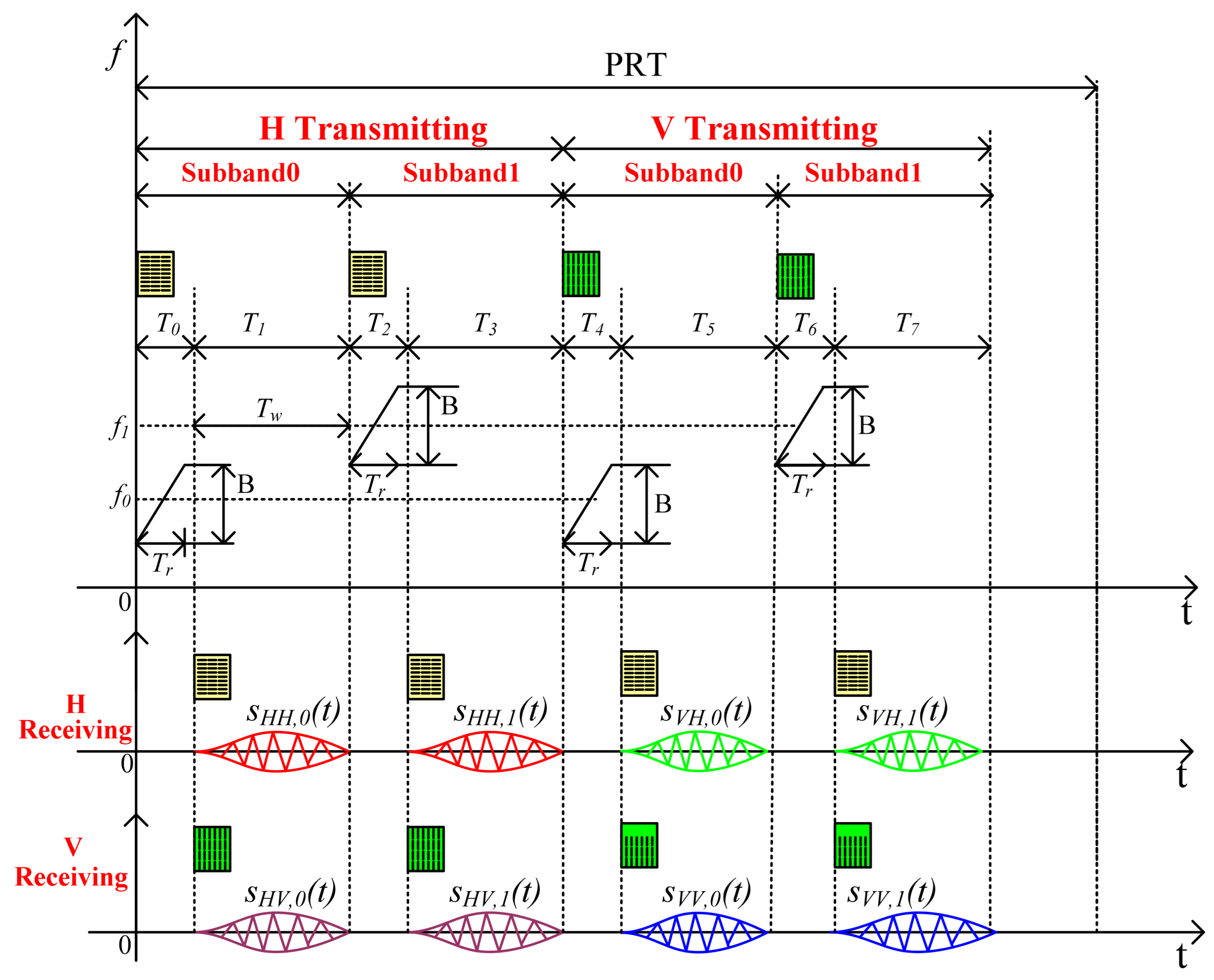
2. The Channel Amplitude and Phase Error Model

The transmission and reception channels of the fully polarimetric airborne SAR system with 0.1 m resolution studied in this project are shown in Figure 1. The signal generated by the signal source is amplified by power and sent to the $H$- and $V$-polarized sub-antennas through two circulators. The echo signals received by the two sub-antennas are then sent to the multichannel receiver through circulators. By switching the transmission channels twice, a fully polarimetric signal can be obtained.

The radar system adopts a time-division working mode, and its timing diagram is shown in Figure 2. The system adopts step-frequency chirps and the center frequencies are $f_0$ and $f_1$, respectively. The bandwidth of the subband signal is $B$ and the pulse width of the transmitted signal is $T_{\mathrm{r}}$. The receiving time window is $T_{\mathrm{w}}$. Each TR cycle includes four subcycles from $T_0$ to $T_7$. In the $T_0$ cycle, $H$-polarized antenna is controlled to transmit the low-frequency subband. In the $T_1$ cycle, the low-frequency subband echoes in $H$ and $V$ polarization, which are denoted as $S_{HH,0}\left(t\right)$ and $S_{HV,0}\left(t\right)$, are received simultaneously. In the $T_2$ cycle, the radar controls the $H$-polarized antenna to transmit the high-frequency subband signal. In the $T_3$ cycle, the high-frequency subband echoes donated as $S_{HH,1}\left(t\right)$ and $S_{HV,1}\left(t\right)$ are received. Similarly, in the $T_4$ and $T_6$ cycle, two subbands are subsequently transmitted through the $V$-polarized antenna. Correspondingly, echoes donated as $S_{VH,0}\left(t\right)$ and ${ S}_{VV,0}\left(t\right)$ are received in the $T_5$ cycle and afterwards $S_{VH,1}\left(t\right)$ and $S_{VV,1}\left(t\right)$ are received in the $T_7$ cycle. By analogy, signal transmission and reception are repeated with period PRT according to the above process within the whole target observation time.

From Figure 2, it can be observed that four transmission and four reception time periods are required to complete a full-polarization and full frequency band data acquisition within one pulse repetition interval. In this scheme, the transmission and reception of low-frequency and high-frequency subband signals are carried out in a time-division manner. Low- and high-frequency subband signals are subsequently generated, power amplified, and then transmitted to two polarized sub-antennas through a ring resonator. In the above stage, nonlinear amplitude and phase modulation are introduced due to the nonlinear characteristics of the device, resulting in amplitude and phase distortion of the signals. Although the internal calibration is performed according to [6], residual sinusoidal amplitude and phase modulation remain in the subband spectrum, which results in prominent paired-echo artifacts and resolution degradation in range. Moreover, unknown linear phase mismatches between the two subbands cannot be controlled by hardware, which brings about the failure to achieve enhanced range resolution after subband synthesis and position distortion between polarized channels. Aiming at obtaining high-quality, high-resolution fully polarimetric images, it is imperative to model and estimate the amplitude and phase errors caused by signal transmission and reception. The following will analyze the modeling of signal amplitude and phase errors.

Without loss of generality, after range compression, the spectrum of the subband signal $S_{p_m,n}^i\left(f_r\right)$ is defined as:

$$S_{p_m,n}^i\left(f_r\right)=A_{p_m,n}^i\left(f_r\right)\mathrm{e}\mathrm{x}\mathrm{p}\left(j{\varnothing }_{p_m,n}^{\epsilon }\left(f_r\right)\right)$$

(1)

$${\varnothing }_{p_m,n}^{\epsilon }\left(f_r\right)={\varnothing }_{p_m,n}^{NL}\left(f_r\right)+{\varnothing }_{p_m,n}^L\left(f_r\right)$$

(2)

$${\varnothing }_{p_m,n}^L\left(f_r\right)=2\pi f_r{\varnothing }_{p_m,n}^1+{\varnothing }_{p_m,n}^0$$

(3)

where $p_m\left(p_m=0, 1, 2, 3\right)$ represents the four polarization channels donated as $HH$, $HV$, $VH$ and VV, $n\left(n=0, 1\right)$ stands for the low-frequency and high-frequency subbands, respectively, $t_r$ and $f_r$, respectively, represent the time and frequency domain vector, $A_{p_m,n}^i\left(f_r\right)$ and ${\varnothing }_{p_m,n}^{\epsilon }\left(f_r\right)$ represent the amplitude spectrum and the phase error in frequency domain of the i-th pulse in the n-th subband, ${\varnothing }_{p_m,n}^{NL}\left(f_r\right)$ represents the nonlinear phase component in ${\varnothing }_{p_m,n}^{\epsilon }\left(f_r\right)$, which results in the generation of paired echoes and defocusing after pulse compression in the subband, and ${\varnothing }_{p_m,n}^L\left(f_r\right)$ represents the linear phase component in ${\varnothing }_{p_m,n}^{\epsilon }\left(f_r\right)$, which affects the initial phase bias and time-domain position offset of the subband compression pulse. Considering the influence on SAR imaging, estimation processes of spectrum amplitude, linear phase, and nonlinear phase errors are introduced in the following section in detail.

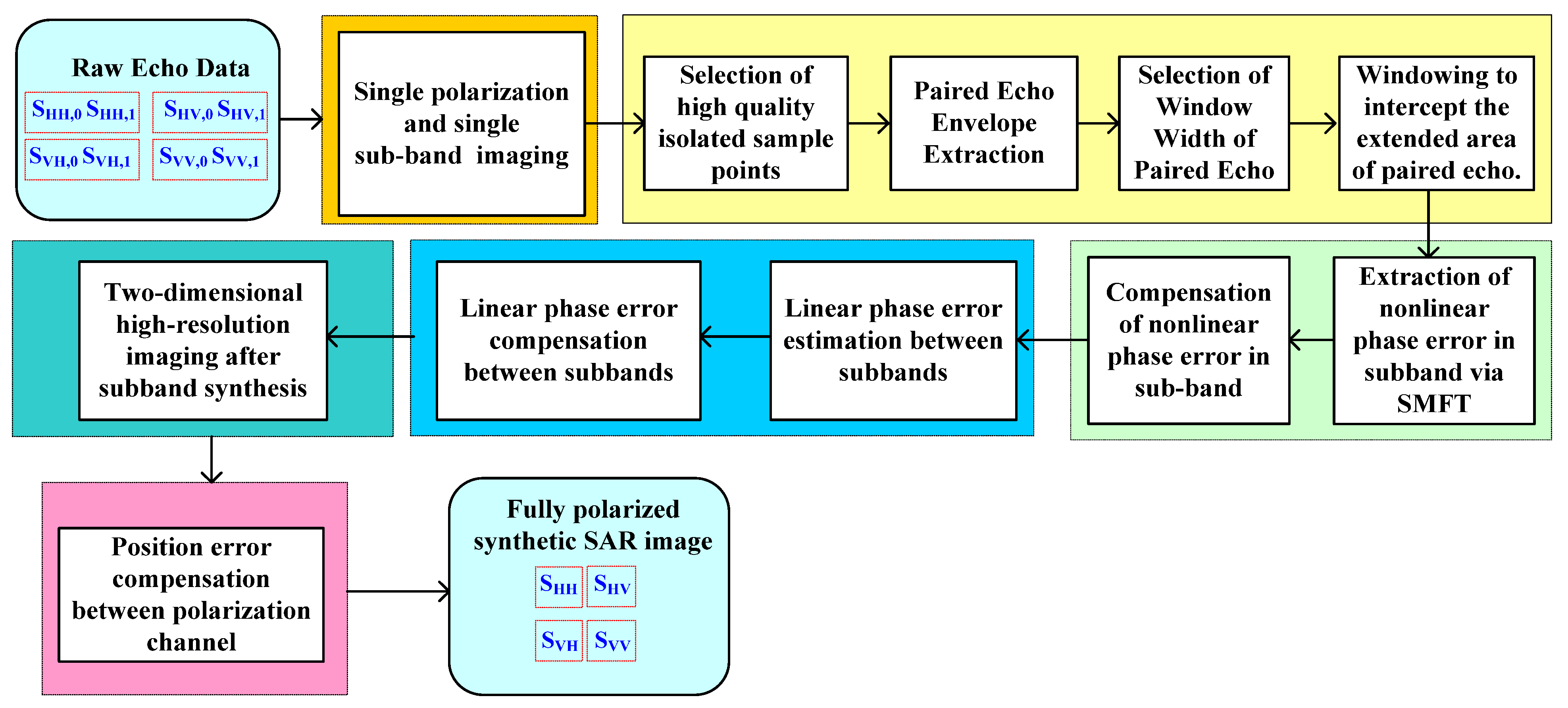
3. Channel Amplitude and Phase Error Estimation

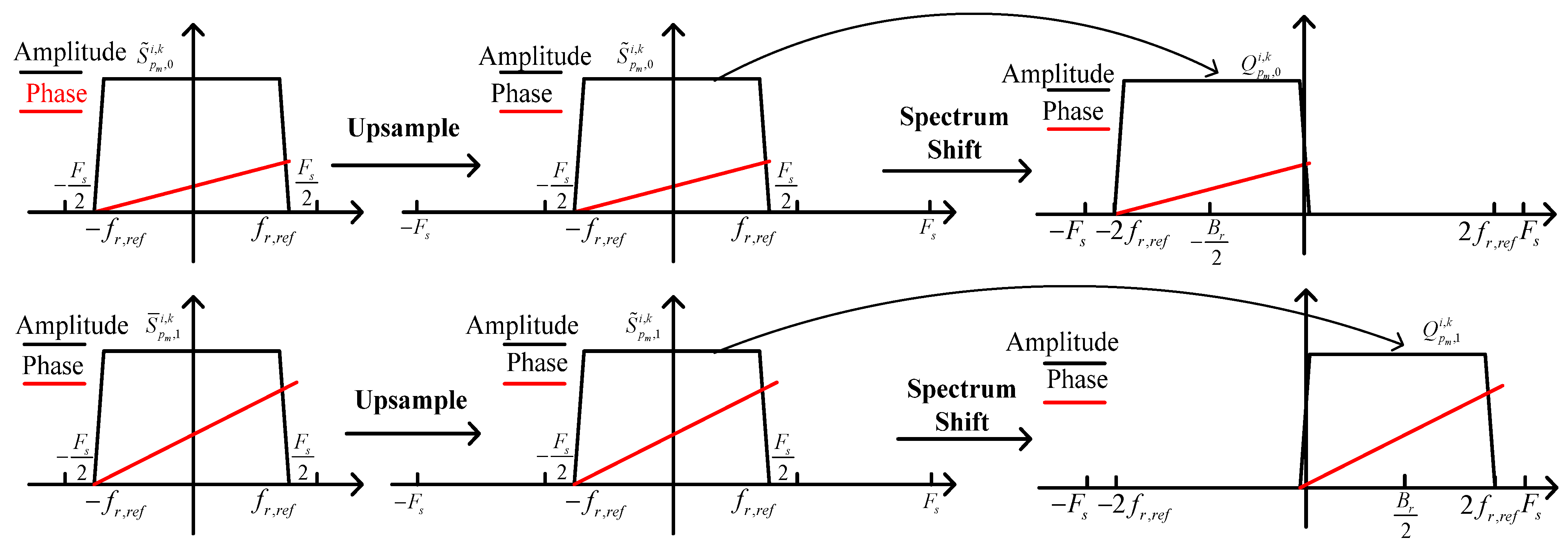
3.1. Estimation of Spectrum Amplitude Distortion Within the Subband

The raw echo data contain signals from various targets, including strongly reflective targets, weakly reflective targets, and uniformly distributed targets. According to statistical laws, the statistical average of massive echo amplitude spectra will gradually approach the true signal amplitude spectrum. Assuming that $S_{p_m,n}^{i,k}$ is a discrete representation of $S_{p_m,n}^i\left(f_r\right)$, where $i=0, 1, \dots ,N_a-1,k=0, 1, \dots ,N_r-1$, $f_r\left(k\right)$ is a discrete representation of $f_r$, $N_r$ and $N_a$ are the number of sampling points in range and azimuth, respectively. The statistical average of the amplitude spectrum of the echo signal could be expressed as:

$${\widehat{A}}_{p_m,n}^k={\widehat{A}}_{p_m,n}\left(f_r\left(k\right)\right)={\displaystyle \frac{1}{N_E}}{\sum }_{i=1}^{N_E}\left|S_{p_m,n}^{i,k}\right|$$

(4)

where ${\widehat{A}}_{p_m,n}^k$ is a discrete representation of ${\widehat{A}}_{p_m,n}\left(f_r\right)$, representing the estimated range amplitude spectrum, and $N_E$ stands for the number of samples used to estimate the spectrum amplitude error.

The process of range amplitude spectrum correction is shown in Figure 3. Assuming $f_r\left(k_{ref}\right)=f_{r,ref}$ and ${\widehat{A}}_{p_m,n}^{k_{ref}}={\widehat{A}}_{p_m,n}\left(f_r\left(k_{ref}\right)\right)$, the amplitude correction reference function $H_{p_m,n}\left(f_r\left(k\right)\right)$ could be designed as follows:

$$H_{p_m,n}^k=\left\{\begin{array}{c}{\displaystyle \frac{{\widehat{A}}_{p_m,n}^{k_{ref}}}{{\widehat{A}}_{p_m,n}^k}},\left|f_r\left(k\right)\right|\le f_{r,ref}\\ 1, other\end{array}\right.$$

(5)

where $[-f_{r,ref},f_{r,ref}]$ represents the effective area of the subband signal spectrum.

Applying the amplitude correction function shown in Equation (5) to correct the original signal amplitude spectrum, the corrected signal spectrum is obtained:

$${{\overline{S}}_{p_m,n}^{i,k}=S}_{p_m,n}^{i,k}{H}_{p_m,n}^k$$

(6)

3.2. Estimation of the Paired-Echo Window Width

Due to the presence of unknown sinusoidal phase errors in the echo spectrum, paired echoes appear in the range-compressed pulse and the final subband image. The distribution characteristic of range paired echoes is determined by the frequency and amplitude of the sinusoidal phase [11]. Due to the migration of the range pulse following the position change in aircraft position and the mutual interference of paired echoes from multiple targets, the expansion curve of paired echoes is difficult to estimate directly.

It is worth noting that after two-dimensional focusing using the subband signal, the target is initially focused in both range and azimuth dimensions and the signal-to-noise ratio of paired-echo components is enhanced. Meanwhile, the interference between paired echoes of the target can be considered negligible. Therefore, we consider finding high-quality isolated strong points from the two-dimensional focused single-sideband image as the samples of nonlinear phase error estimation. It should be noted that the range and azimuth dimensions should not be windowed during initial imaging to avoid amplitude weighting of the sample data.

Considering that the larger the backscattering coefficient of a target, the higher its signal-to-noise ratio, the phase error extracted from the point target is closer to the true value. Furthermore, the fewer targets around a single strong target, the less affected it is by the amplitude and phase errors of surrounding targets. Based on these considerations, this article adopts a highest-contrast criterion [24] to select error estimation samples. Assuming that the subband signal after amplitude spectrum correction is ${\overline{S}}_{p_m,n}^{i,k}$, and the result image of two-dimensional imaging is $I_{p_m,n}^{i,j}$, the estimation procedure of the paired echo window width is shown in Figure 4, which mainly includes the following steps:

Step 1: Calculate the average value ${\mu }_{p_m,n}^i={\displaystyle \frac{1}{N_r}}{\sum }_{j=1}^{N_r}{\left|I_{p_m,n}^{i,j}\right|}^2$ and deviation value ${\sigma }_{p_m,n}^i={\displaystyle \frac{1}{N_r}}{\sum }_{j=1}^{N_r}{\left({\left|I_{p_m,n}^{i,j}\right|}^2-{\mu }_{p_m,n}^i\right)}^2$ for each range line in the subband image $I_{p_m,n}^{i,j}$, then the contrast of each range line would be obtained as $C_{p_m,n}^i={\displaystyle \frac{{\rho }_{p_m,n}^i}{{\mu }_{p_m,n}^i}}$.

Step 2: Sort all the contrast value $C_{p_m,n}^i$ in descending order and obtain the descending contrast curve $C_{p_m,n}^i$. By setting the threshold ${ϵ}_{p_m,n}=k_{p_m,n}\times max\left(C_{p_m,n}^i\right)$ of high-quality samples according to the threshold selection scheme in [25], all range lines with a contrast greater than ε are selected as high-quality sample.

Step 3: Normalize the peak amplitude of the selected high-quality range line and then shift the peak point of each sample to the center position of range lines.

Step 4: Average the amplitude of the peak-aligned sample range lines to eliminate the influence of noise and distributed weak targets, the averaged curve $A_{p_m,n}^j$ is obtained.

Step 5: Process the averaged curve $A_{p_m,n}^j$ obtained from Step 4 by windowed smoothing, the range expansion function curve with a smooth envelope would be expressed as $E_{p_m,n}^j={\sum }_{k=-{\displaystyle \frac{W_s}{2}}}^{{\displaystyle \frac{W_s}{2}}}{A}_{p_m,n}^{j+k}$, where $W_s$ stands for the width of smoothing window.

Step 6: Search the peak positions of the first paired echoes, which are donated as $P_L$ and $P_R$ with distance n₁ and n₂ from the center point, respectively. According to the position distribution characteristic of paired echoes [11], the window width of the paired echo would be calculated as: $W_{p_m,n}=4\times \mathrm{m}\mathrm{a}\mathrm{x}\left(\right[n_1 n_2\left]\right)$.

Step7: Go to Step 1 unless all the subbands with different polarization modes are processed.

3.3. In-Band Nonlinear Phase Error Estimation

The residual nonlinear component ${\mathrm{\varnothing }}_{p_m,n}^{NL}\left(f_r\right)$ is mainly manifested in the form of a sinusoidal signal, resulting in paired echoes of the time-domain compression pulse, which has a small impact on the image cost function. Moreover, the energy expansion function curve is not monotonically decreasing, making it difficult to extract phase errors using the cost function or phase-gradient-based methods. Inspired by the azimuth high-frequency vibration error estimation algorithm [18,19], the form of the phase error appearing in the subband spectrum and the phenomenon of paired echoes closely resemble those caused by platform vibration. Therefore, high-quality reference points can be extracted from the image, and the sine modulation Fourier transform (SMFT) method can be used to extract in-band nonlinear phase errors, which is shown in Figure 5. A nonlinear phase error in the form of sine series can be modeled as follows:

$$\mathrm{e}\mathrm{x}\mathrm{p}\left({j\varnothing }_{p_m,n}^{NL}\left(f_r\right)\right)=exp\left(j{\sum }_{v=0}^V{C}_{v}exp\left(j2\pi {\displaystyle \frac{v}{F_s}}{f}_r\right)\right)$$

(7)

where $F_s$ represents the range sampling rate.

The group delay function of the frequency domain phase error is:

$$D_{p_m,n}\left(f_r\right)={\displaystyle \frac{1}{2\pi }}{\displaystyle \frac{d}{d{f}_r}}{\varnothing }_{p_m,n}^{NL}\left(f_r\right)$$

(8)

The Fourier transform of the above equation yields:

$$FFT\left[D_{p_m,n}\left(f_r\right)\right]=Re\left\{{\displaystyle \frac{j\omega }{2\pi }}FT\left[{\varnothing }_{p_m,n}^{NL}\left(f_r\right)\right]\right\}=-Im\left\{{\displaystyle \frac{\omega }{2\pi }}FFT\left[{\varnothing }_{p_m,n}^{NL}\left(f_r\right)\right]\right\}$$

(9)

By organizing the above equation, we obtain:

$$D_{p_m,n}\left(f_r\right)=-Im\left\{IFFT\left[{\displaystyle \frac{\omega }{2\pi }}FFT\left[{\varnothing }_{p_m,n}^{NL}\left(f_r\right)\right]\right]\right\}=-Im\left\{IFFT\left[{\displaystyle \frac{\omega }{2\pi }}SFMFT\left(S_{p_m,n}\left(f_r\right)\right)\right]\right\}$$

(10)

In the discrete frequency domain, Equation (7) can be expressed as:

$$\mathrm{e}\mathrm{x}\mathrm{p}\left({j\varnothing }_{p_m,n}^{NL}\left(f_r\right)\right)=exp\left(j{\sum }_{v=0}^V{C}_{v}exp\left(j2\pi v{\displaystyle \frac{k}{N_r}}\right)\right)$$

(11)

where $C_v$ is the complex coefficient, and $N_r$ is the number of range sampling points under discrete conditions.

Performing a discrete sine frequency Fourier transform on Equation (11) yields:

$$\mathrm{S}\mathrm{F}\mathrm{M}\mathrm{F}\mathrm{T}\left(\mathrm{e}\mathrm{x}\mathrm{p}\left({j\varnothing }_{p_m,n}^{NL}\left(f_r\right)\right)\right)=FFT\left(-jln\left(S_{p_m,n}\left(k\right)\right)\right)$$

(12)

where $W_M=exp\left(-j{\displaystyle \frac{2\pi }{N_r}}\right)$ is the complex coefficient.

By combining Equations (8) and (11), we can obtain:

$$D_{p_m,n}\left(k\right)=-Im\left\{IFFT\left[f_r\left(k\right)FFT\left(-jln\left(S_{p_m,n}\left(k\right)\right)\right)\right]\right\}$$

(13)

After obtaining the group delay of the phase error, the nonlinear phase error within the subband can be obtained by integration:

$${\varnothing }_{p_m,n}^{NL}\left(k\right)=\left\{\begin{array}{c}0,k=0\\ 2\pi {\sum }_{j=0}^k{D}_{p_m,n}\left(j\right), 1\le k\le N_r-1\end{array}\right.$$

(14)

The main steps of estimating the nonlinear phase error within the subband include:

Step 1: For $L_{p_m,n}$ point targets in the $p_m,n$ mode, the range compression pulse with the width of $W_{p_m,n}$ is extracted with the coordinate $(i_k,j_k)$ as the center, and the two ends complement each other $\left({N_r-W}_{p_m,n}\right)/2$, we get ${\tilde{p}}_{p_m,n}^l\left(m\right), m=0, 1, \dots ,N_r-1$.

Step 2: According to Equations (10)–(14), the nonlinear phase error estimation value ${\widehat{\varnothing }}_{p_m,n}^{NL,l}\left(k\right)$ is obtained by SMFT processing of ${\tilde{p}}_{p_m,n}^l(m)$.

Step 3: The estimated value of the nonlinear phase error ${\widehat{\varnothing }}_{p_m,n}^{NL,l}\left(k\right)$ is statistically averaged, and the estimated value of the nonlinear phase error of the channel is ${\widehat{\varnothing }}_{p_m,n}^{NL}\left(k\right)={\displaystyle \frac{1}{L_{p_m,n}}}{\sum }_{l=0}^{L_{p_m,n}-1}{\widehat{\varnothing }}_{p_m,n}^{NL,l}\left(k\right)$.

Step 4: The nonlinear phase error compensation of the range signal spectrum ${\overline{S}}_{p_m,n}^{i,k}$ is carried out, and is the following is obtained ${\tilde{S}}_{p_m,n}^{i,k}={\overline{S}}_{p_m,n}^{i,k}·exp\left(-j{\widehat{\varnothing }}_{p_m,n}^{NL}\left(k\right)\right)$.

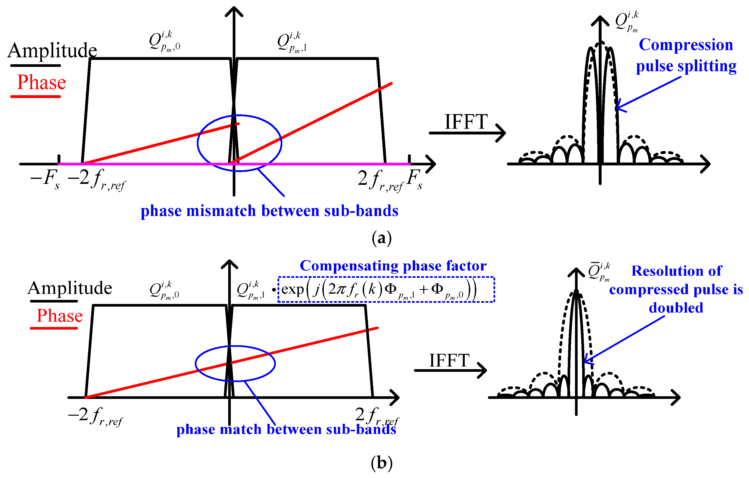
3.4. Linear Phase Error Estimation Between Subbands

After the estimation of the nonlinear phase error in high- and low-frequency bands of each polarization channel is completed, the residual linear phase error between subbands is still unknown. Although it will not affect the focusing characteristics of subband compressed pulses, it will affect the fixed phase offset and focusing position of subband compressed pulses. These imperfections ultimately degrade the focusing quality of compressed pulses after band synthesis. It is necessary to accurately estimate the inter-subband linear phase error.

Before error estimation and compensation, it is necessary to carry out upsampling and spectrum shifting on subband signal spectra ${\tilde{S}}_{p_m,0}^{i,k}$ and ${\tilde{S}}_{p_m,1}^{i,k}$, as shown in Figure 6. The sampling rate after upsampling is $F_{s2}={2F}_s$, and the shifted spectrum is $Q_{p_m,0}^{i,k}$ and $Q_{p_m,1}^{i,k}$.

If the linear phase error between subbands is not compensated, it will lead to the phenomenon shown in Figure 7a, where the compressed pulse would split and defocus after subband synthesis and the range resolution cannot be doubled.

As shown in Figure 7b, taking the subband frequency band $Q_{p_m,1}^{i,k}$ as a reference, the linear phase of the subband frequency spectrum $Q_{p_m,0}^{i,k}$ is compensated and the following results are obtained:

$${\overline{Q}}_{p_m}^{i,k}=Q_{p_m,0}^{i,k}exp\left(j{\Phi }_{p_m}\left(k\right)\right)+Q_{p_m,1}^{i,k}$$

(15)

$${\mathsf{\Phi }}_{p_m}\left(k\right)=2\pi f_r{\varphi }_{p_m,1}+{\varphi }_{p_m,0}$$

(16)

$${\overline{q}}_{p_m}^{i,n}={\displaystyle \frac{1}{N_r}}{\sum }_{k=0}^{{2N}_r-1}{\overline{Q}}_{p_m}^{i,k}exp\left(j{\displaystyle \frac{2\pi }{N_r}}nk\right)$$

(17)

In Equation (16), the variable ${\varphi }_1$ is the coefficient of the linear term, which affects the position of the compression pulse, and ${\varphi }_0$ is the initial phase of the linear term, which affects the consistency of the phases between subbands. ${\varphi }_1$ and ${\varphi }_0$ are unknown variables, which need accurate estimation and compensation to ensure that the resolution of compressed pulses after subband synthesis is doubled.

Considering the adaptability of the objective function to different scenes, we choose the information entropy $E_{p_m}$ of the sample compressed pulse image as the cost function:

$$E_{p_m}=-{\sum }_{i=0}^{I-1}{\sum }_{n=0}^{{2N}_r-1}{\displaystyle \frac{{\left|{\overline{q}}_{p_m}^{i,n}\right|}^2}{E_z}}ln\left({\displaystyle \frac{{\left|{\overline{q}}_{p_m}^{i,n}\right|}^2}{E_z}}\right) ={\displaystyle \frac{1}{E_z}}{\sum }_{i=0}^{I-1}{\sum }_{n=0}^{{2N}_r-1}{\left|{\overline{q}}_{p_m}^{i,n}\right|}^{2}ln\left({\left|{\overline{q}}_{p_m}^{i,n}\right|}^2\right)-ln\left(E_z\right)$$

(18)

$$E_z={\sum }_{i=0}^{I-1}{\sum }_{n=0}^{{2N}_r-1}{\left|{\overline{q}}_{p_m}^{i,n}\right|}^2$$

(19)

where ${\left|{\overline{q}}_{p_m}^{i,n}\right|}^2$ represents the pixel brightness, $E_z$ represents the total signal energy, and $I$ represents the number of sample compression pulses.

An optimal estimation model of two-dimensional vector ${\varphi }_{p_m}={\left[{\varphi }_{p_m,1},{\varphi }_{p_m,0}\right]}^T$ is established by taking the image information entropy $E_{p_m}$ as the objective function:

$${\widehat{\varphi }}_{p_m}=argmin{E}_{p_m}\left({\varphi }_{p_m,1},{\varphi }_{p_m,0}\right)$$

(20)

Equation (20) is an unconstrained optimization problem, which requires an accurate derivation of the objective function-variable gradient analytical formula.

Combining Equations (16)–(18), the gradient variable of pixel brightness ${\left|{\overline{q}}_{p_m}^{i,n}\right|}^2$ to the variable vector ${\mathsf{\Phi }}_{p_m}\left(k\right)$ is expressed as:

$${\displaystyle \frac{{\partial \left|{\overline{q}}_{p_m}^{i,n}\right|}^2}{\partial {\mathsf{\Phi }}_{p_m}\left(k\right)}}={\displaystyle \frac{1}{N_r}}IM\left({\left(Q_{p_m,0}^{i,k}\right)}^{\mathrm{*}}exp\left(-j{\mathsf{\Phi }}_{p_m}\left(k\right)\right){\overline{q}}_{p_m}^{i,n}exp\left(-j{\displaystyle \frac{2\pi }{N_r}}nk\right)\right)$$

(21)

Combine Equations (16)–(19) to find the gradient of the total image energy $E_z$ to variable vector $\mathsf{\Phi }\left(k\right)$:

$${\displaystyle \frac{\partial E_z}{\partial {\mathsf{\Phi }}_{p_m}\left(k\right)}}={\displaystyle \frac{1}{N_r}}{\sum }_{i=0}^{I-1}IM\left({\left(Q_{p_m,0}^{i,k}\right)}^{\mathrm{*}}exp\left(-j{\mathsf{\Phi }}_{p_m}\left(k\right)\right)Q_{p_m,1}^{i,k}\right)$$

(22)

Combine Equations (18)–(22) to find the gradient of the image information entropy $E_{p_m}$ to variable vector ${\mathsf{\Phi }}_{p_m}\left(k\right)$:

$${\displaystyle \frac{\partial E_{p_m}}{\partial {\mathsf{\Phi }}_{p_m}\left(k\right)}}=-{\displaystyle \frac{1}{N_r{E}_z}}{\sum }_{i=0}^{I-1}IM\left({\left(Q_{p_m,0}^{i,k}\right)}^{\mathrm{*}}exp\left(-j{\mathsf{\Phi }}_{p_m}\left(k\right)\right)Z_{p_m}^{i,k}\right)$$

(23)

$$Z_{p_m}^{i,k}={\sum }_{n=0}^{{2N}_r-1}{\overline{q}}_{p_m}^{i,n}ln{\displaystyle \frac{{\left|{\overline{q}}_{p_m}^{i,n}\right|}^2}{E_z}}exp\left(-j{\displaystyle \frac{2\pi }{N_r}}nk\right)+E_{p_m}{\overline{Q}}_{p_m}^{i,k}$$

(24)

where the intermediate variable $Z_{p_m,i}^{i,k}$ can be quickly calculated by FFT.

Combining the Expressions (17) and (23), we can obtain the gradient variables of the objective function $E_{p_m}$ to the variables ${\varphi }_{p_m,1}$ and ${\varphi }_{p_m,0}$:

$${\displaystyle \frac{\partial E_{p_m}}{\partial {\varphi }_{p_m,1}}}= -{\displaystyle \frac{1}{N_r{E}_z}}{\sum }_{i=0}^{I-1}IM\left[{\sum }_{k=0}^{N_r-1}{\left({\overline{Q}}_{p_m}^{i,k}\right)}^{\mathrm{*}}{\left(Z_{p_m,i}^{i,k}\right)}^{\mathrm{*}}{f}_r\left(k\right)\right]$$

(25)

$${\displaystyle \frac{\partial E_{p_m}}{\partial {\varphi }_{p_m,0}}}=-{\displaystyle \frac{1}{N_r{E}_z}}{\sum }_{i=0}^{I-1}IM\left[{\sum }_{k=0}^{N_r-1}{\left({\overline{Q}}_{p_m}^{i,k}\right)}^{\mathrm{*}}{Z}_{p_m,i}^{i,k}\right]$$

(26)

With the objective function given by Equation (18) and the gradient vector given by Equations (25) and (26), the optimal estimate of the error vector ${\widehat{\varphi }}_{p_m}=[{\widehat{\varphi }}_{p_m,1},{\widehat{\varphi }}_{p_m,0}]$ can be quickly solved by using unconstrained optimization algorithm. Substituting ${\widehat{\varphi }}_{p_m}$ into Equation (16), we get the optimal estimation of the linear phase error between frequency bands ${\widehat{\mathsf{\Phi }}}_{p_m,i}\left(k\right)=2\pi f_r{\widehat{\varphi }}_{p_m,1}+{\widehat{\varphi }}_{p_m,0}$. Finally, the frequency spectrum ${\overline{Q}}_{p_m}^{i,k}$ synthesized by two channels after linear phase error compensation and the range compression pulse ${\widehat{q}}_{p_m}^{i,n}$ with double resolution can be obtained from Equations (15) and (17).

$${\widehat{Q}}_{p_m}^{i,k}=Q_{p_m,0}^{i,k}exp\left(j{\widehat{\mathsf{\Phi }}}_{p_m,i}\left(k\right)\right)+Q_{p_m,1}^{i,k}$$

(27)

$${\widehat{q}}_{p_m}^{i,n}={\displaystyle \frac{1}{N_r}}{\sum }_{k=0}^{{2N}_r-1}{\widehat{Q}}_{p_m}^{i,k}exp\left(j{\displaystyle \frac{2\pi }{N_r}}nk\right)$$

(28)

3.5. Estimation of Position Deviation Between Polarized Channels

After the subband synthesis of each polarization channel is completed, according to the imaging geometric relationship combined with the velocity, position and attitude parameters measured by the motion sensor, a unified imaging coordinate system is constructed to perform motion compensation and imaging processing on the original data. Then the high-resolution complex SAR image $Y_{p_m}^{i,n}$ of each polarization channel is obtained. Because the amplitude and phase errors between polarization channels are quite different, after subband synthesis, there is obvious deviation in the position of images between polarization channels, which needs to be accurately corrected.

In order to reduce the computational complexity, the high-quality sample point coordinate set $G_{p_m,n}$ in Section 3.2 is used to select the image slice ${ss}_{p_m}^{i,n}$ with a size of $N_{sa}\times N_{sr}$, whose center position locate at [$i_1,j_1$]. Without loss of generality, taking $HH$ channel $\left(p_m=0\right)$ as the reference channel, two-dimensional cross-correlation is implemented as:

$$R_{p_m,0}={IFFT}_2\left({FFT}_2\left(\left|{ss}_{p_m}^{i,n}\right|\right){FFT}_2^{\mathrm{*}}\left(\left|{ss}_0^{i,n}\right|\right)\right),p_m=1, 2, 3$$

(29)

By searching the peak position $\left[i_{max},n_{max}\right]$ of the two-dimensional correlation function $R_{p_m,0}$ and carrying out two-dimensional time-domain translation on the corresponding polarization channel, accurate registration of polarized images can be realized.

3.6. Computational Complexity Analysis of the Algorithm

The data processing flow of this project is mainly shown in Figure 8.

The fully polarized radar system studied in this paper consists of eight subband signals, covering four polarizations and two subband spectrums. The number of sampling points in the single-channel subband signal is $N_a\times N_r$, and after double-upsampling and subband synthesis the number is increased to $N_a\times {2N}_r$. Considering floating-point complex multiplication, the results of computational complexity analysis of the proposed algorithm are listed in

Table 1. Computational complexity of the algorithm.

Operation of Algorithm	Step of Algorithm	Quantity	Computational Complexity
Correction of subband spectrum amplitude	Range FFT of subband signal *	8 channels	${4N}_a{N}_r{log}_2{(N}_r)$ *
	Average amplitude spectrum		${8N}_E{N}_r$
	Subband spectrum amplitude correction *		${8N}_a{N}_r$ *
Estimation of paired-echo window width	Calculate contrast of range line	8 channels	${5N}_a{N}_r$
	Normalize amplitude of high-quality line		$8{L_{p_m,n}N}_r$
Correction of in-band nonlinear phase error	Nonlinear phase error estimation in subband	8 channels	$8L_{p_m,n}{N_r(log}_2{(N}_r)+1)$
	Nonlinear phase error compensation in subband *		${8N}_a{N}_r$ *
Correction of linear phase error between subbands	Phase error compensation	4 channels L iterations	$8I{N}_{r}L$
	IFFT of synthesized spectrum		${\left(4{IN}_r\right)log}_2\left(2N_r\right)L$
	Calculate image entropy		$8{IN}_{r}L$
	Calculate intermediate variables		${\left(4I{N}_r\right)(log}_2\left(2N_r\right)+2)L$
	Calculate gradient		$24I{N}_{r}L$
	Linear phase error compensation *	4 channels	${8N}_a{N}_r$ *
Correction of position deviation between polarized channels	2D FFT of image sample	4 channels	${{2N}_{sa}N}_{sr}\left({log}_2\right(N_{sr})+{log}_2(N_{sa}\left)\right)$
	Conjugate multiplication		${{3N}_{sa}N}_{sr}$
	2D IFFT of the result of conjugate multiplication		${{2N}_{sa}N}_{sr}\left({log}_2\right(N_{sr})+{log}_2(N_{sa}\left)\right)$
Computational complexity for estimation	$(8N_E+5N_a)N_r+8\left({log}_2\left(N_r\right)\right)+2)L_{p_m,n}{N}_r+(48+8{log}_2\left(2N_r\right))I{N}_{r}L+(4{log}_2\left(N_{sr}\right)+4{log}_2\left(N_{sa}\right)+3){N_{sa}N}_{sr}$
Other computational complexity *	$(24+4{log}_2{(N}_r))N_a{N}_r$

*: Necessary for imaging, computation complexity is not included in the algorithm.

.

In order to facilitate the computation analysis, the number of range lines for subband spectrum amplitude error estimation is assumed as $N_E=N_a/128$. Similarly, the number of high-quality samples for estimation of the paired-echo window width and the phase error is assumed as ${L_{p_m,n}=N}_a/128$ and ${I=N}_a/128$. Moreover, the average iteration number of the algorithm is set as $L=8$. Furthermore, the size of the single-polarized sub-block image are defined as ${ N}_{sa}={ N}_a/4$ and $N_{sr}=N_r/4$. The total computational complexity for error estimation shown in Table 1 can be redefined as:

$$N_{est}={\displaystyle \frac{{13log}_2\left(N_r\right)+4{log}_2\left(N_a\right)+110}{16}}{N_{a}N}_r$$

(30)

The other computational complexity listed in Table 1 can be expressed as:

$$N_{other}=(24+4{log}_2{(N}_r))N_a{N}_r$$

(31)

In the actual SAR system, the number of range sampling points Nr = 32,768 and that of azimuth $N_a=8192$. Substituting the above parameters into (31) and (32), the proportional coefficient of calculation complexity is obtained as follows:

$${\displaystyle \frac{N_{est}}{N_{other}}}={\displaystyle \frac{{13log}_2\left(N_r\right)+4{log}_2\left(N_a\right)+110}{16(24+4{log}_2{(N}_r))}}=0.2656$$

(32)

It can be seen from Equation (32) that the computation of the error estimation algorithm is only about 1/4 of other necessary computations, which shows that the computation of the error estimation algorithm is a very small part of the imaging algorithm.

4. Experimental Results

4.1. Fully Polarimetric Airborne SAR with 0.1 m Resolution

The main parameters of the radar system studied in this paper are shown in

Table 2. System parameter list.

Technical Parameter	Technical Parameter Value
Center frequency	15 GHz
Polarization channel number	4
Subband pulse width	20 µs
Flight altitude	3000 m
Subband bandwidth	800 MHz
Total bandwidth	1600 MHz
Number of subbands	2
detection range	>10 km

. The radar operates in Ku-band and fully polarimetric design is adopted. Each polarized channel transmits two subband signals with a bandwidth of 800 MHz, the total bandwidth is 1600 MHz and the radar detection range exceeds 10 km.

The original echo data will be processed according to the signal processing flow shown in Figure 8, and the processing results of each step are shown in detail.

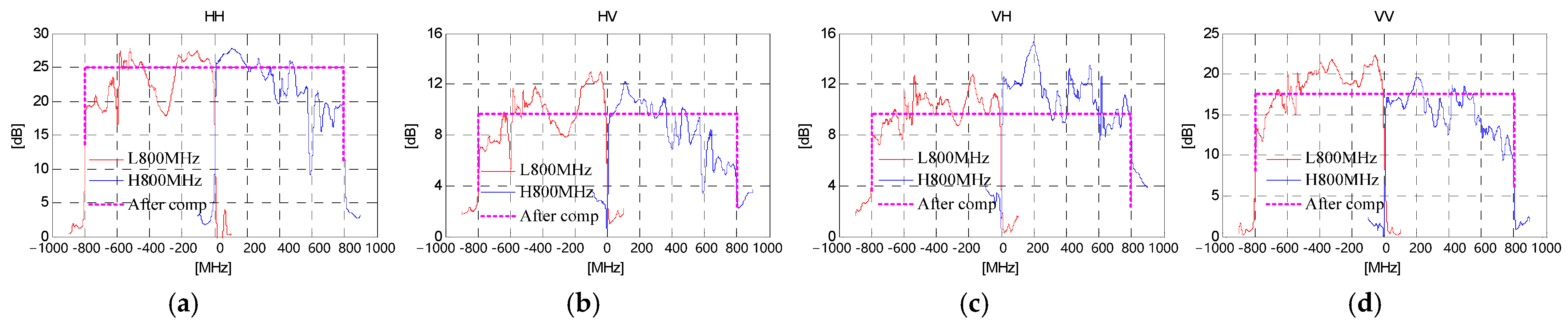
4.1.1. Subband Spectrum Amplitude Correction for Fully Polarimetric Airborne SAR

According to Formula (4), the amplitude spectra of the high and low subbands in the $HH$, $HV$, $VH$, and $VV$ polarizations are statistically accumulated, and the results of spectral amplitude compensation is shown in Figure 9a–d. In order to highlight the differences of the amplitude spectrum of high and low subbands, the amplitude spectra of subband signals are positioned at the central frequencies of −400 MHz and 400 MHz, respectively. In Figure 9, the red solid line is the amplitude spectrum of the low-frequency subband and the blue solid line is that of the high-frequency subband. According to Formula (4), the correction curve of the amplitude spectrum of each subband is calculated, and the dotted pink line indicating the corrected amplitude spectral curve.

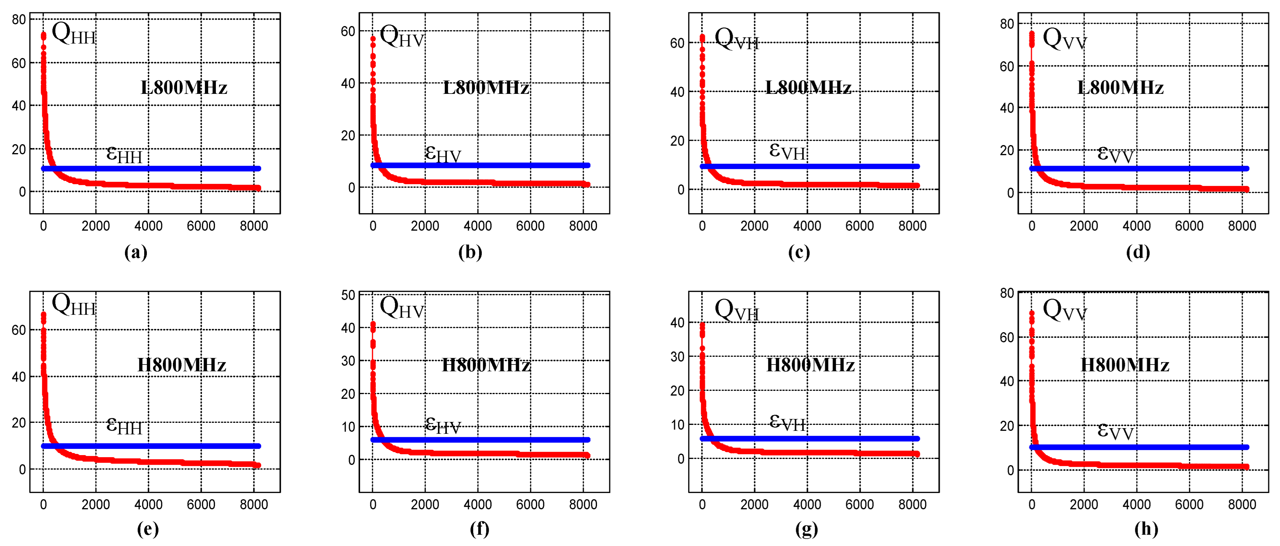
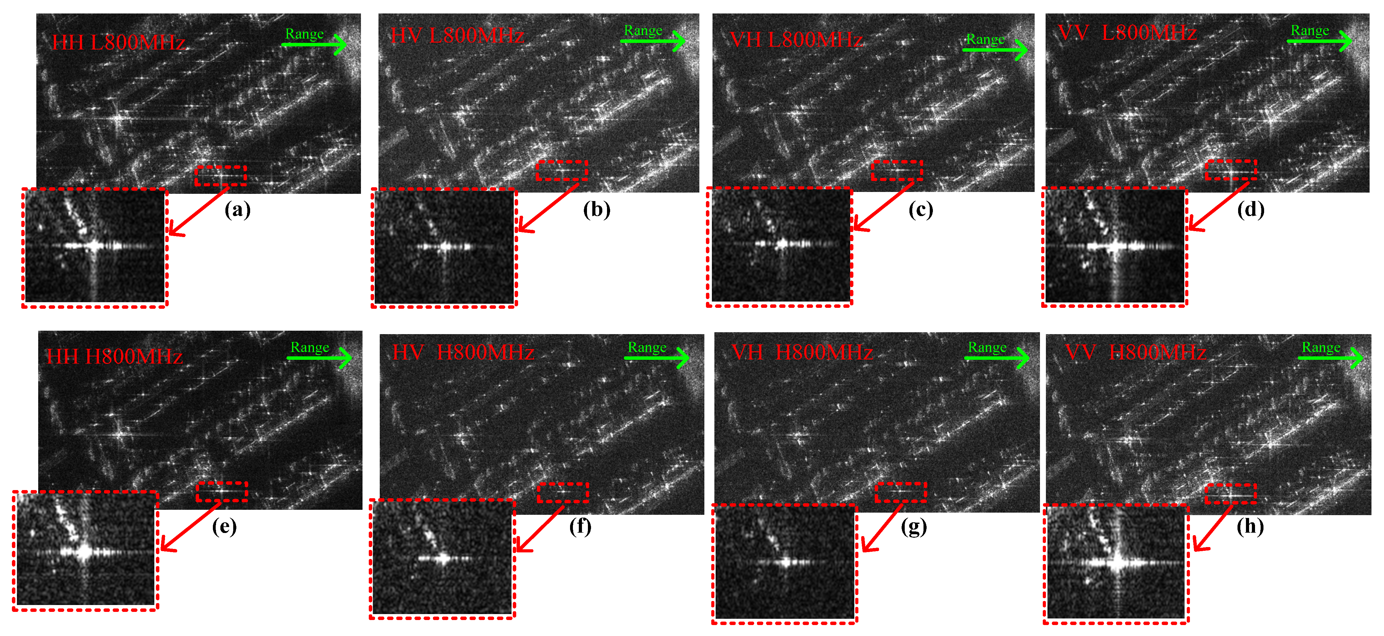
4.1.2. Selection of High-Quality Dominant Points and Determination of the Window Width of the Expansion Curve

After amplitude correction, the subband signal spectrum is processed to obtain single-polarized SAR. By setting threshold ${ϵ}_{p_m,n}=0.15\times max\left(C_{p_m,n}^i\right)$ shown in Figure 10a–h, high-quality range lines containing isolated paired echoes, which are circled by red markers in Figure 11a–h could be selected for the following process.

By setting the width of smoothing window $W_s=2$ and performing smoothing processing twice, the paired-echo spread function could be obtained according to Figure 4. Figure 12a–h show the selection of paired-echo window widths, where the red solid line represents the normalized accumulated sample amplitude curve, the blue solid line corresponds to the smoothed sample amplitude curve, and the pink dotted line indicates the spreading area of paired echoes.

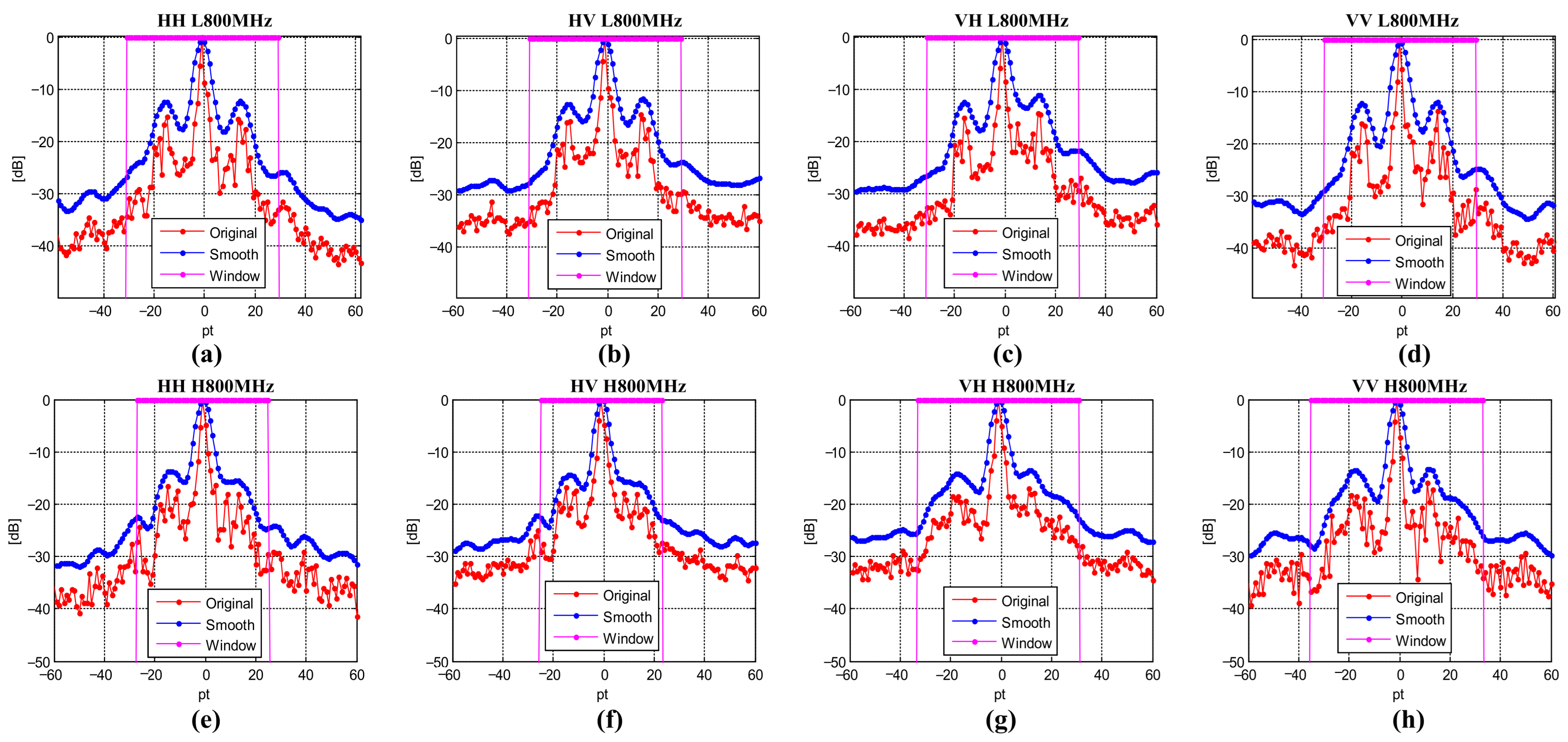
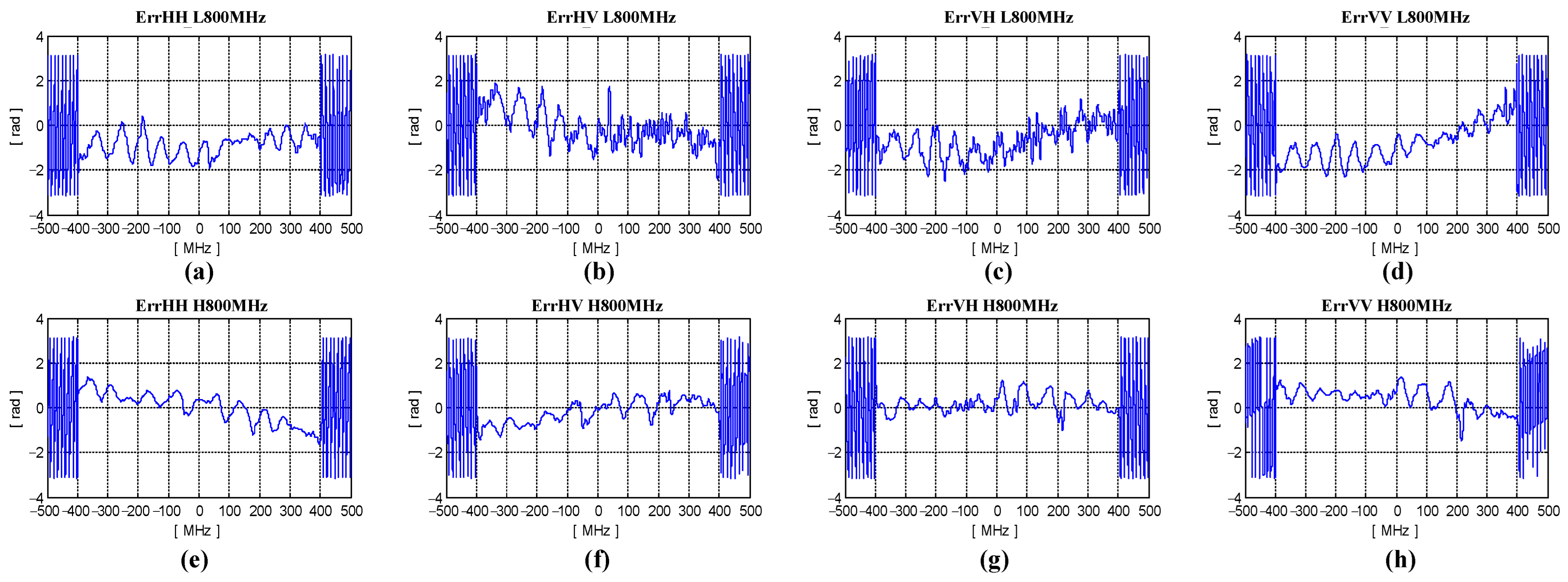
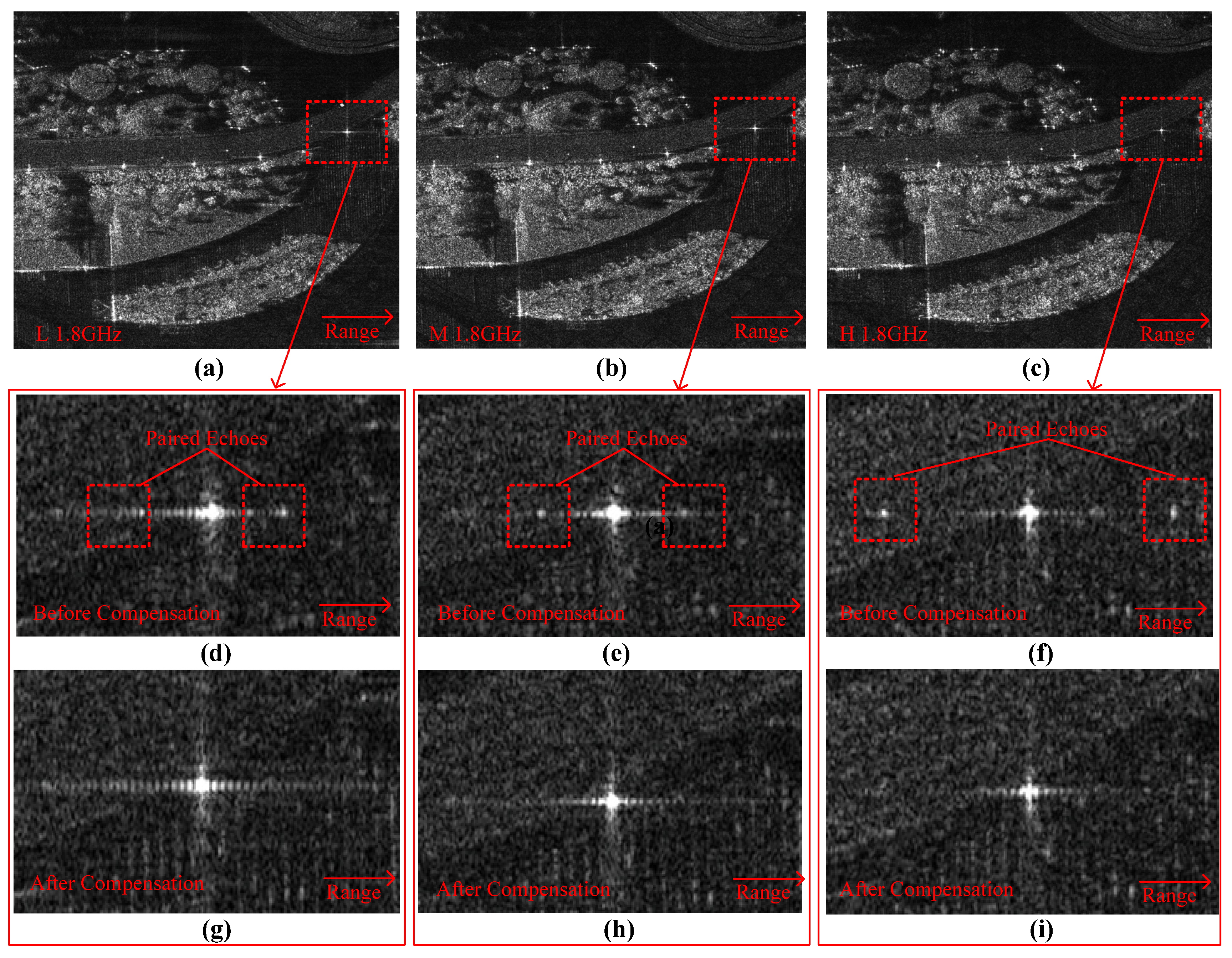
4.1.3. Nonlinear Phase Error Estimation for Fully Polarimetric Airborne SAR

In order to observe the detailed characteristics of the paired echoes of point targets, Figure 13a–h show the imaging results without nonlinear phase error compensation, where the horizontal and vertical axes represent the range and the azimuth directions, respectively. In addition, the red box in the image is an isolated strong reflection point target, which is used to observe the imaging quality and quantitatively assess the range resolution. From the imaging results presented in Figure 13a–h, we find that the paired-echo phenomenon of point targets is distinctly obvious, which leads to misjudgment of the real target position.

According to Section 3.3, the nonlinear phase error in the subband is analyzed with the estimated nonlinear phase error curve shown in Figure 14a–h. It can be observed that the nonlinear phase error manifests as an irregular sinusoidal series, with an amplitude deviation range primarily between ±2.0 rad. Moreover, the phase error curves are distributed within the frequency band from −400 MHz to 400 MHz and exhibit random variations outside the effective frequency band.

By compensating the nonlinear phase error shown in Figure 13a–h, the imaging performance of the subband is shown in Figure 15a–h. Comparing Figure 15a–h with Figure 13a–h, it can be seen that the image focusing performance is significantly improved after error compensation. Additionally, the phenomenon of range paired echoes has completely disappeared and the position of the point target can be clearly identified.

The amplitude envelope curves of the point targets in the box area with and without error compensation are extracted and shown in Figure 16a–h, where the blue solid line represents the range amplitude envelope without compensation and the red solid line stands for that with compensation. Without error compensation, the envelope of paired echoes is significantly apparent. After phase error compensation, the focusing effect of the point targets shows clear improvement and paired echoes disappear completely, which directly proves that the nonlinear error compensation is effective.

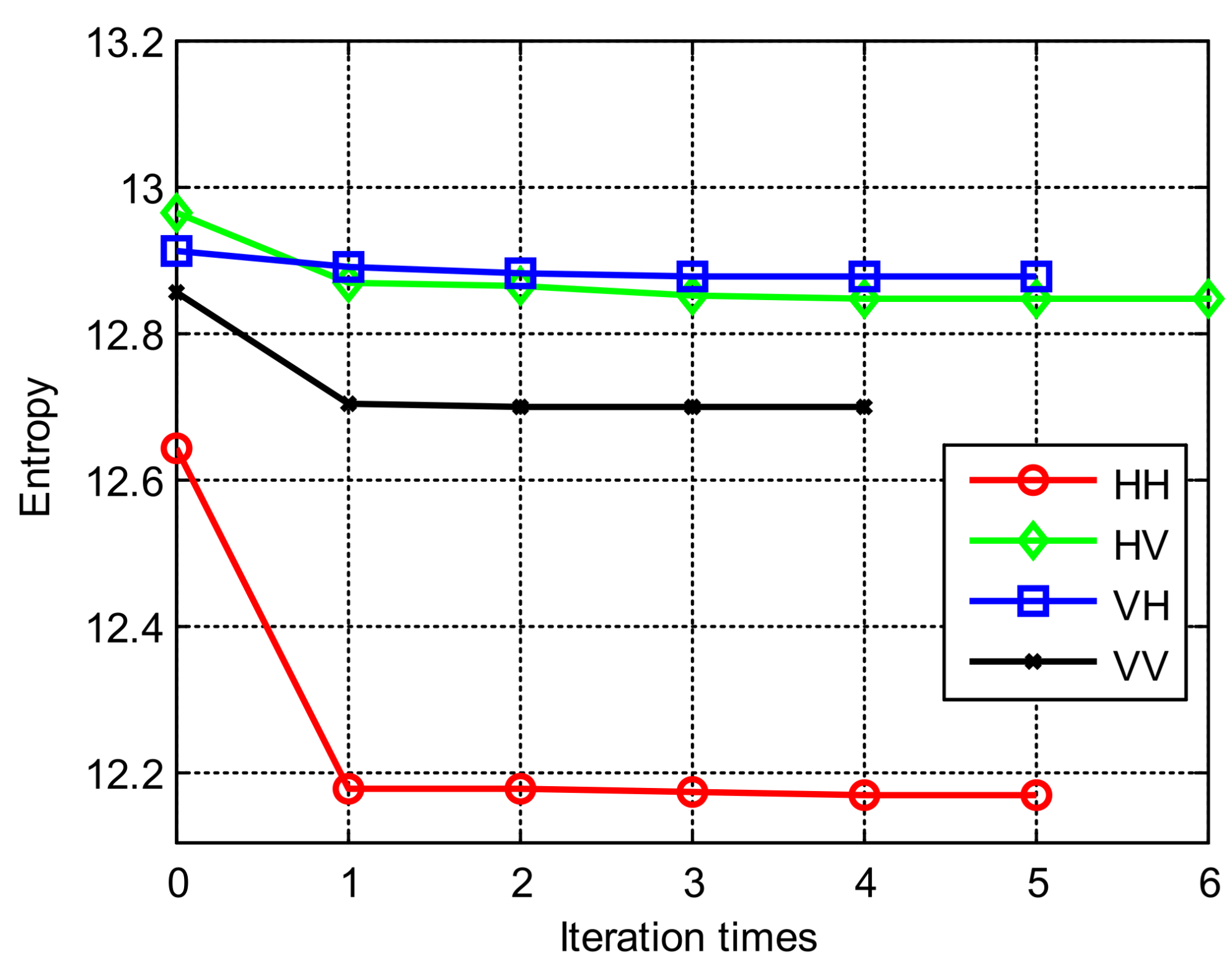
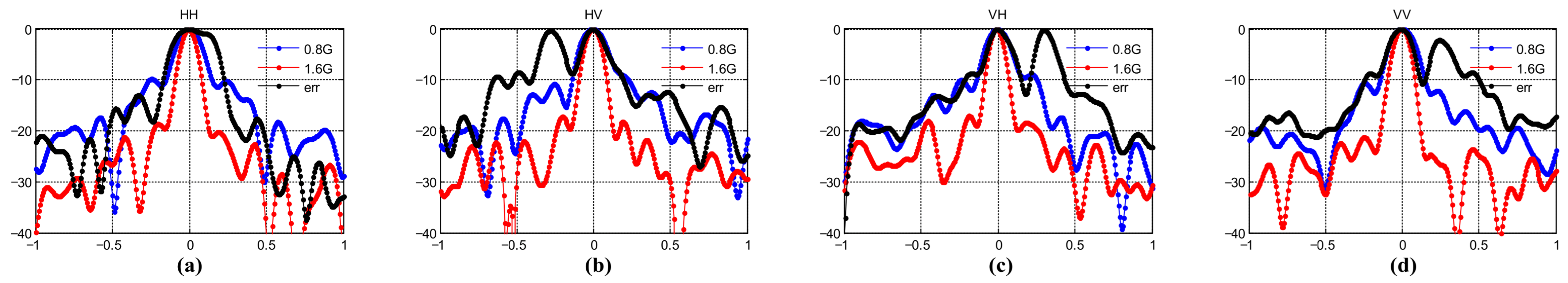
4.1.4. Linear Phase Error Estimation Between Subbands

Considering that the convergence speed and position of unconstrained optimization are closely related to the spatial distribution characteristics of the objective function, it is necessary to examine the three-dimensional spatial distribution characteristics of the objective function before error estimation. Assuming variable ${\varphi }_{p_m,0}({\varphi }_{p_m,0}\in \left[-\pi ,\pi \right])$ to be the X axis, variable ${\varphi }_{p_m,1}$(${\varphi }_{p_m,1}\in [-4/F_{s2},4/F_{s2}]$) to be the Y axis and the objective function $E_{p_m}\left({\varphi }_{p_m,0},{\varphi }_{p_m,1}\right)$ to be Z axis, it can be seen in Figure 17a–d that the objective function of the two-dimensional solution exhibits strong local convexity characteristics, and the distribution of contour lines near the optimal point is also very clear. Therefore, the unconstrained optimization algorithm can be used to solve the parameter estimation problem efficiently.

Under the computer configuration with 13th Gen Intel i7-13700H CPU and working frequency at 2.4 GHz, all the channel errors are estimated by using the fminunc function on MATLAB (v2021) software platform. With ${\varphi }_{p_m}={\left[0,0\right]}^T$ as the initial search point and $\epsilon =0.001$ as the iterative convergence threshold, the iterative search curve of the objective function for unconstrained optimal estimation of linear phase errors is shown in Figure 18. From the four curves in Figure 18, it can be seen that the algorithm approaches very close to the optimal solution after one iteration, and can quickly converge to the optimal solution within 6 iterations, indicating that the selected cost function exhibits excellent local convergence characteristics.

Table 3. Computational time for linear phase error estimation between subbands.

Polarization Mode	Computational Time for Linear Phase Error Estimation Between Subbands (s)
HH	0.1104
HV	0.1275
VH	0.1178
VV	0.1065
Total computational time	0.4622

shows the time spent in estimating the linear phase error between channels. From Table 3, it can be seen that the time consumed by a single channel is basically consistent with the iterative curve in Figure 18, and the total time spent in estimating the linear phase error of all four channels is 0.4622 s. Under the airborne condition, the whole system only needs to estimate the linear phase error once, which is basically negligible for the whole strip flight.

Taking a local isolated strong target as an example, Figure 19a–h show the contrast effect of range-compressed pulse images before and after the synthesis of four single-polarization mode frequency bands. By comparing Figure 19a,e, Figure 19b,f, Figure 19c,g and Figure 19d,h, it can be seen that the width of the range-amplitude envelope is reduced by 50% after error compensation, indicating a significant improvement in the range resolution.

After linear phase error compensation and subband synthesis, the imaging result of the local area is shown in Figure 20a–d. As can be seen from Figure 20a–d, the single-polarization imaging effect after subband synthesis achieves excellent performance, with the detailed information of the image being abundantly preserved, and an outstanding two-dimensional focusing effect observed for the point target in the box area.

Figure 21a–d show the comparison of range envelopes of point targets after frequency band synthesis. In the figure, the blue solid line is the single-band range amplitude envelope, the black solid line is the range amplitude envelope before error compensation, and the red solid line is the range amplitude envelope after error compensation. By comparing and analyzing the four curves, it can be seen that the resolution of range compression pulse of the point target synthesized by direct frequency band before error compensation has not been improved, but the envelope has widened and split. After error compensation, the range pulse width of the point target is reduced to half that of the single subband, and the improvement in range resolution is significant.

Table 4. Comparison of point target resolution indexes of frequency band synthesis before and after error compensation.

Polarization Mode	Subband Range Resolution (m)	Synthesized Range Resolution Without Compensation (m)	Synthesized Range Resolution with Compensation (m)
HH	0.1827	0.2833	0.0979
HV	0.1800	0.1332	0.0985
VH	0.1800	0.1530	0.0981
VV	0.1875	0.1450	0.0982

shows the comparison results of point target range resolution before and after error compensation in the rectangular area in Figure 20a–d. It can be seen from the table that the point target resolution of direct frequency band synthesis without error compensation has not improved and has even deteriorated. After the error compensation, the range resolution is doubled, and the range resolution of the single-polarization full-band achieves better than 0.1 m, which meets the system design specifications. It can be seen that the amplitude and phase error estimation algorithm proposed in this paper is effective.

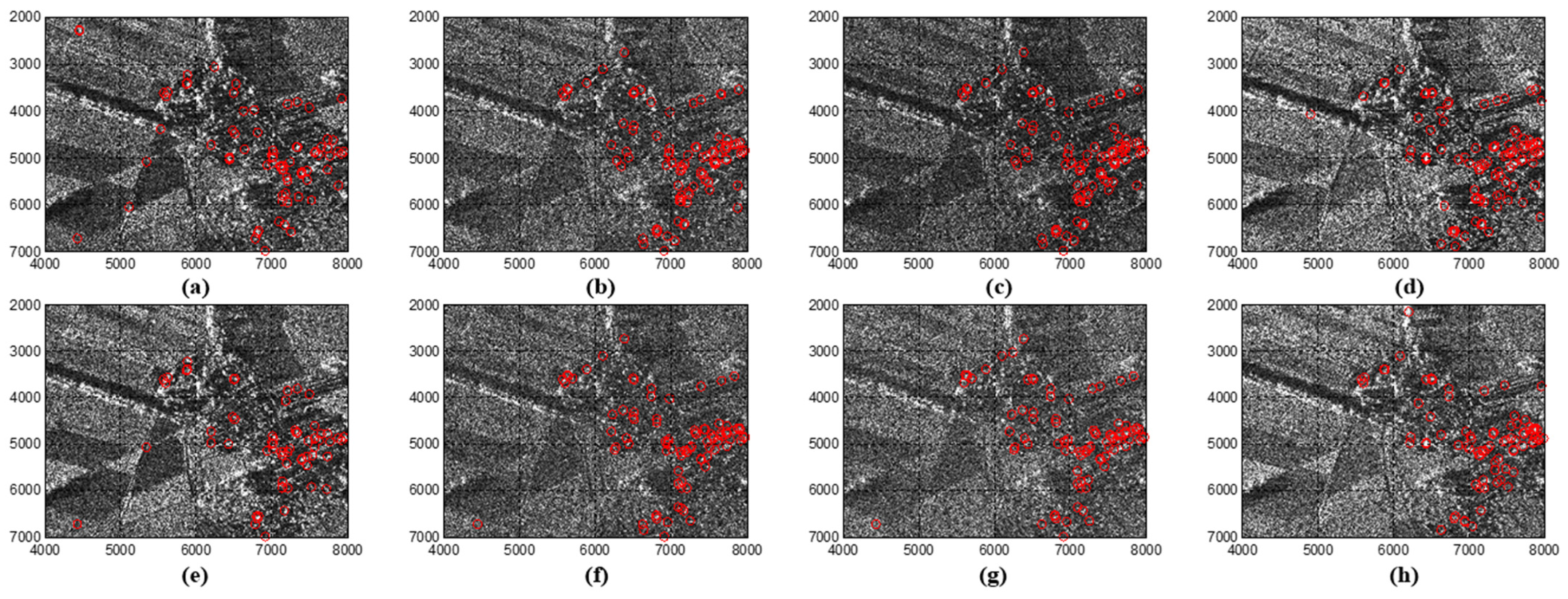
4.1.5. Estimation of Position Error Between Polarization Channels

After all the subband spectra are synthesized, the same motion sensor parameters are used for motion compensation and imaging processing [26,27]. Nonlinear and linear phase error compensation results in unknown position deviation in each polarization channel, which can be estimated following Section 3.5. By selecting a image slice located at the point with the highest amplitude and shifting the position of the non-reference channel according to the result of two-dimensional correlation, a fully polarimetric SAR image with aligned target positions can be obtained.

Figure 22a–b show the effects of fully polarimetric images before and after position error compensation. The $Red$ color stands for the $VV$ polarization channel, the $Green$ color stands for the $HH$ polarization channel, and the $Blue$ color stands for the mean value of the $HV$ and $HV$ polarization channels. After RGB color synthesis, the imaging result before and after position compensation are shown in Figure 22. Comparing Figure 22b with Figure 22a, it can be observed that the target pixels are obviously aligned and the position of typical objects can be identified easily.

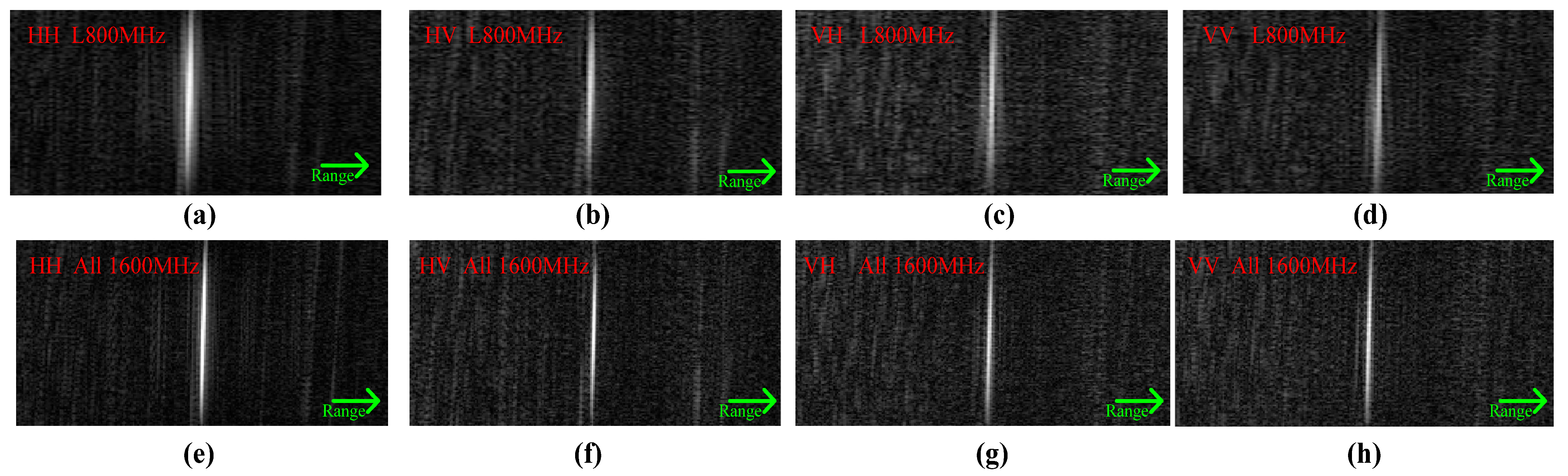
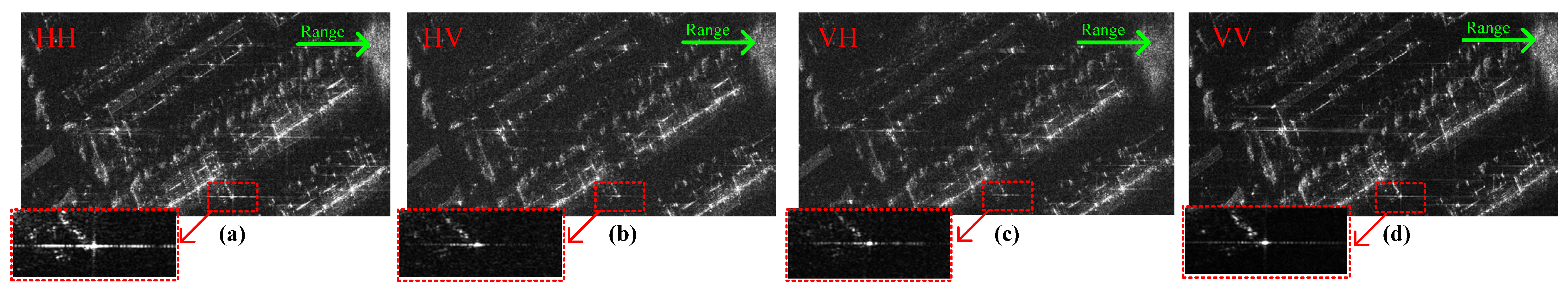
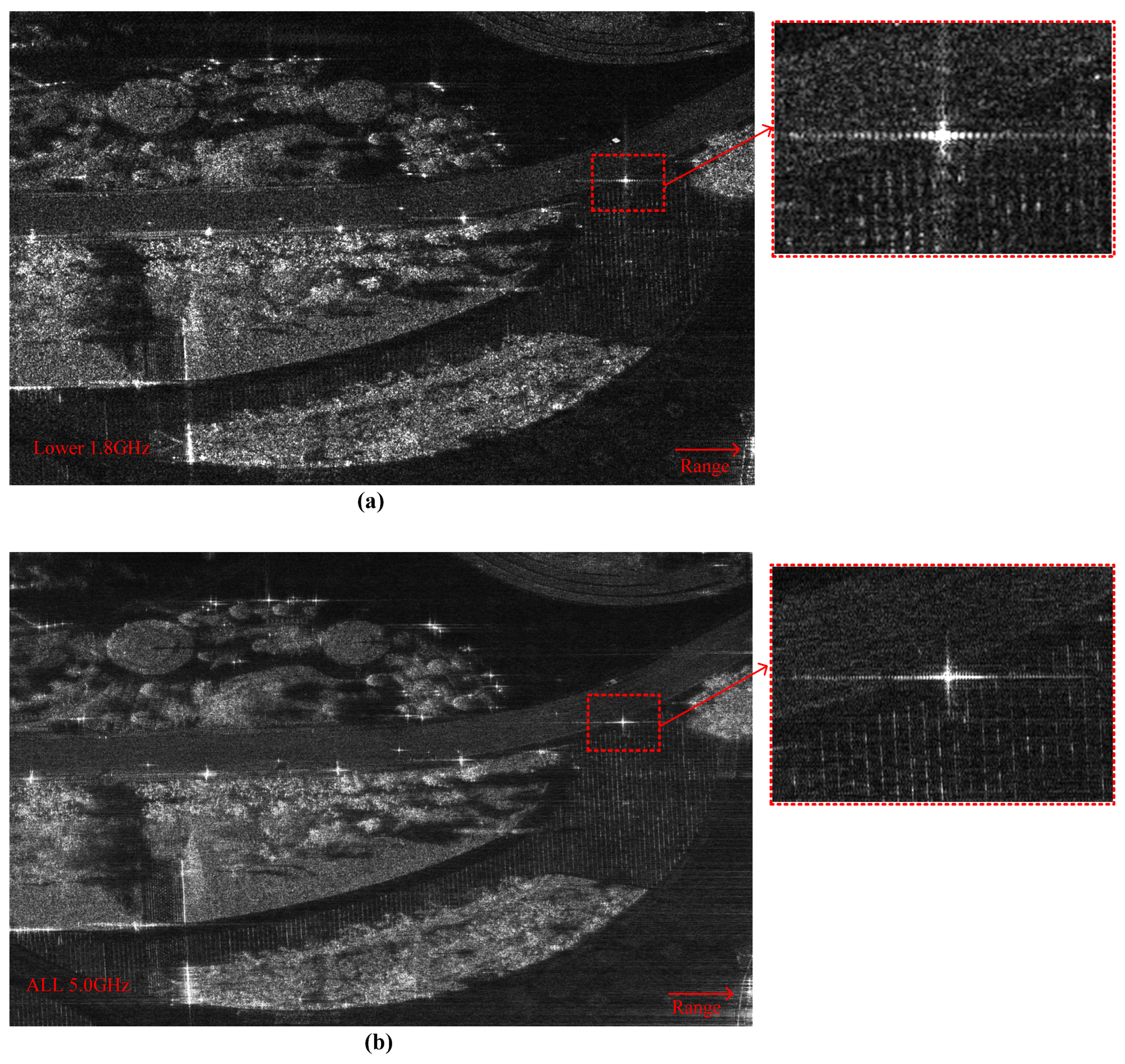
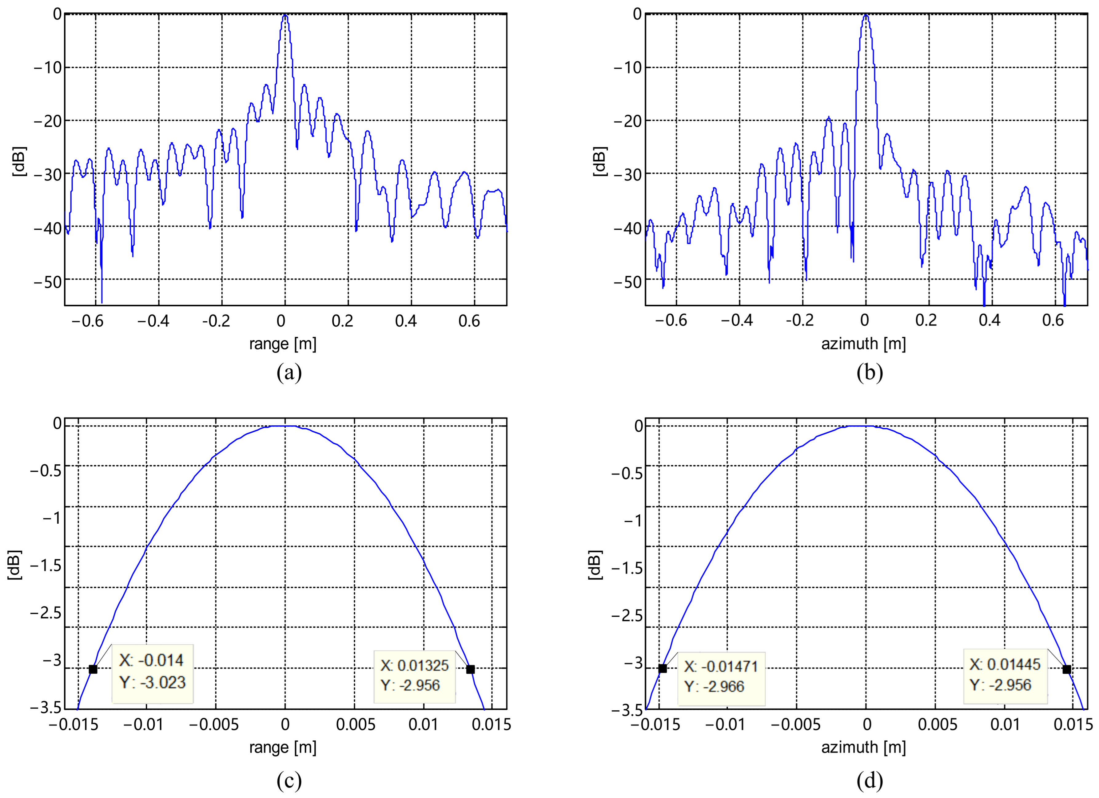
4.1.6. Fully Polarimetric Imaging After Amplitude and Phase Error Compensation

By compensating the amplitude, the nonlinear phase error, the linear phase error between subbands and the position error between polarization channels, a high-quality fully polarimetric airborne SAR image with 0.1 m resolution is obtained in Figure 23.

The image scene mainly includes farmland, roads, houses and highways. On the one hand, the resolution of the image is very high and the detailed information of ground objects is very delicate and clear. On the other hand, the polarization characteristics of farmland regional targets are very obvious, and the color information after pseudo-color coding is very rich, which can clearly distinguish different crop classification situations. By synthesizing the effects of wide-area, large-range, high-resolution and fully polarimetric imaging, it can be seen that the amplitude and phase error calibration algorithm based on echo data proposed in this paper is very effective and can solve the problem of accurate estimation of error information such as amplitude, phase and position of radar echo data.

4.2. Ultrahigh-Resolution Single Polarimetric Airborne SAR with a 0.03 m Resolution

The main parameters of another ultrahigh-resolution single polarimetric airborne SAR system are listed in

Table 5. Parameter list of the ultrahigh-resolution SAR system.

Technical Parameter	Technical Parameter Value
Center frequency	15 GHz
Polarization mode	VV
Work pattern	Strip-map/Spotlight
Subband pulse width	10 µs
Flight altitude	2500 m
Subband bandwidth	1.8 GHz
Total bandwidth	5.0 GHz
Number of subbands	3
Resolution	0.03 × 0.03 m
detection range	>10 km

. The center frequency of SAR system is 15 GHz and single polarimetric design is adopted. Three subband signals are transmitted and received successively in VV polarization mode. Moreover bandwidths of all the subbands are 1.8 GHz uniformly, and there is a certain overlap between subband spectra. After subband synthesis the total bandwidth is 5 GHz, and the final two-dimensional resolution of the system is 0.03 × 0.03 m in the spotlight mode.

Similarly, the results of data processing will be described in detail below.

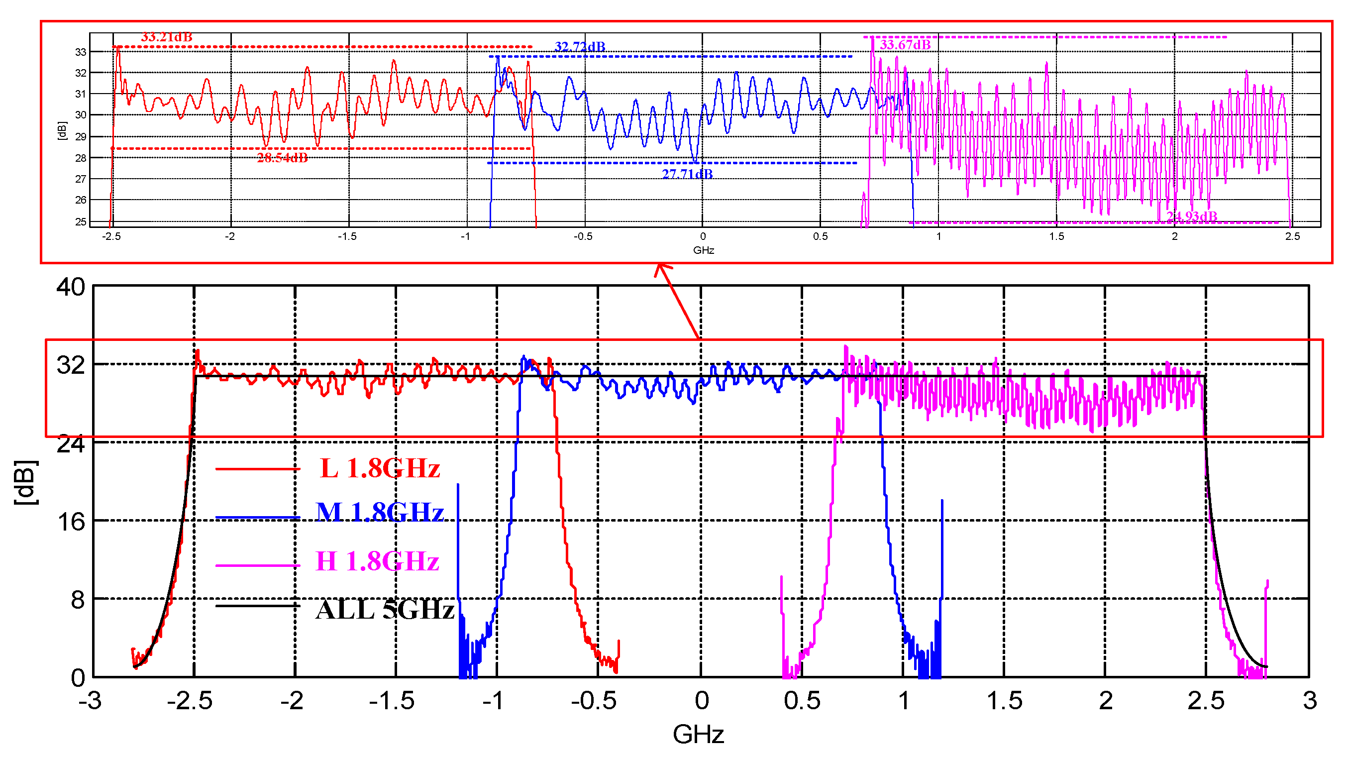
4.2.1. Subband Spectrum Amplitude Correction for Ultrahigh-Resolution Airborne SAR

The amplitude spectra of subband echoes are statistically averaged to obtain the subband spectral envelope curve as shown in Figure 24. It can be seen from the figure that there is an overlapping area with spectral interval 160 MHz between subbands, and the bandwidth range after spectrum synthesis is [−2.5 GHz, 2.5 GHz]. Within each subband bandwidth interval, the spectrum amplitude fluctuates in different degrees. By observing the enlarged local area shown in Figure 24, it can be seen that the spectrum amplitude of the three subbands varies in the range of 4.67 dB, 5.01 dB and 8.74 dB, respectively. Furthermore, there are obvious amplitude modulations in sinusoidal forms, where the modulation frequency is the highest and the modulation amplitude is the largest in the third subband. After amplitude correction, the spectral amplitude of subband is close to the ideal rectangular window shape, which is shown in the solid black line in the figure.

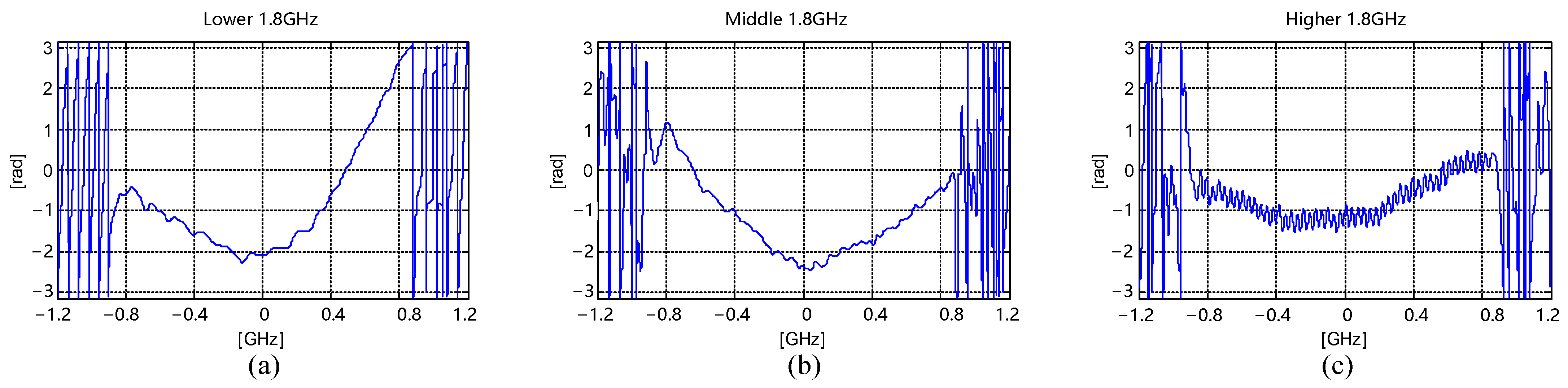
4.2.2. Nonlinear Phase Error Estimation in the Subband for Ultrahigh-Resolution Airborne SAR

The subband images obtained by processing subband signals, respectively, defocus slightly in range and contain obvious paired echo targets. According to the method in Section 3.2, it is necessary to find high-quality isolated strong points in subband images. Figure 25a–c show the results of independent imaging of three subbands, where high-quality sample points are circled in red. By comparing the position of sample points shown in Figure 25a–c, it can be seen that the position of the sample points in the three subband images are basically consistent, which shows that the results of high-quality sample point are relatively stable.

The results of nonlinear phase error estimation in subbands are shown in Figure 26a–c. It can be seen that the phase errors shown in Figure 26a,b contain mainly low-frequency phase components, and the curve is close to the quadratic function, which would bring about defocusing of range-compressed pulse and weak paired echoes. The phase error shown in Figure 26c contains mainly high-frequency phase components, which would lead to more powerful paired echoes.

After nonlinear phase error compensation, the results of subband imaging are shown in Figure 27a–c. This scene is a typical leisure square in urban environment, and the two-dimensional focusing effect of the image is very good, and the outline of the ground green belt, trees, road, street lamp and other targets could be clearly identified. The natural point target in the rectangular area in the subband image is extracted. Figure 27d–f shows the amplification effect of the point target before error compensation. The point target in the figure is defocused to a certain extent, and the effect of paired echoes is very obvious. The distance between the paired echoes in the third subband is twice that of the first two subbands, which is consistent with the distribution form of the error function. As shown in Figure 27g–i, after compensation the two-dimensional focusing effects of point targets have been significantly improved, where the paired echoes have been well suppressed.

4.2.3. Linear Phase Error Estimation Between Subbands for Ultrahigh-Resolution Airborne SAR

After compensation of the nonlinear phase error in the subband, the schematic diagram of subband synthesis effect is shown in Figure 28. Firstly, the three subband spectrums are upsampled by 2.5-fold interpolation. Secondly, the lower subband spectrum is shifted to the central frequency of −1.6 GHz to obtain ${\mathrm{S}}_1\left(k\right)$, and the higher subband spectrum is shifted to the central frequency of 1.6 GHz to obtain ${\mathrm{S}}_3\left(k\right)$, the middle subband spectrum ${\mathrm{S}}_2\left(k\right)$ keep unchanged. Thirdly, the linear phase error ${\mathsf{\Phi }}_{\mathrm{1,2}}\left(k\right)$ between the lower and the middle subband is estimated according to Section 3.4, and then the linear phase error ${\mathsf{\Phi }}_{\mathrm{2,3}}\left(k\right)$ between the middle and the higher subband is estimated. Finally, after error compensation, all the three subbands are combined to obtain the full-bandwidth spectrum as follows.

$${\mathrm{S}}_{ALL}\left(k\right)={\mathrm{S}}_1\left(k\right)e^{-j{\Phi }_{\mathrm{1,2}}\left(k\right)}+{\mathrm{S}}_2\left(k\right)+{\mathrm{S}}_3\left(k\right)e^{-j{\Phi }_{\mathrm{2,3}}\left(k\right)}$$

(33)

The imaging effects of single-band and full-band synthesis in the strip-map mode are shown in Figure 29a,b. By contrast, it can be seen that after band synthesis, the detailed information of the ground target in the imaging scene is richer and the peripheral outline of the target is clearer. The natural isolated point target shown in the rectangular area is extracted and enlarged to be visible, where the range mainlobe envelope is three times thinner after subband synthesis. Moreover, the width of the white bright line formed by the gap in the bottom plate of the leisure square is also obviously reduced, where the effect of range resolution improvement is very remarkable.

In order to improve the azimuth resolution, a flight test in the spotlight mode was carried out on the basis of subband synthesis, and correspondingly, a spotlight SAR image was obtained in Figure 30. The focusing effect of this image is very good, ground targets such as stadium, roads and trees are very clear, and the texture of the leisure square ground can also be recognized. In order to quantitatively analyze the two-dimensional resolution of the image, the natural strong point targets in the red rectangular area are extracted and the two-dimensional amplitude envelopes are upsampled by 100-fold interpolation, where the original and 3 dB enlarged local envelopes of point A could be shown in Figure 31a–d. Two-dimensional resolution of the point targets are calculated in

Table 6. Two-dimensional resolution of point targets.

Point Target	Range Resolution (m)	Azimuth Resolution (m)
A	0.0273	0.0292
B	0.0286	0.0282
C	0.0280	0.0285
D	0.0271	0.0291
E	0.0288	0.0289
Average value	0.0280	0.0288

, which meets the system resolution requirement of 0.03 × 0.03 m.

5. Discussion

Aiming at the problems of paired echoes and range defocusing in a fully polarized airborne SAR system with 0.1 m resolution, the algorithm proposed in this paper has achieved a very good imaging effect. It should be noted that the algorithm relies on the selection of high-quality isolated strong points in the estimation procedure of the nonlinear phase error. Without isolated strong points in the scene, the effect of the algorithm will be greatly affected.

Following the development of integrated circuit technology, the analog input bandwidth, sampling frequency and sampling bit number of ADC will be improved; correspondingly, the two-channel subband synthesis can be directly replaced by single-channel sampling. However, it is worth noting that a high resolution is the eternal pursuit of radar system design; therefore, channel amplitude and phase error estimation for subband synthesis is an effective technical proposal to achieve a higher imaging resolution under insufficient hardware performance. The algorithm proposed in this paper is universal and can be applied to multi-platform airborne radar systems with higher the resolution.

6. Conclusions

In this paper, we address two critical challenges in fully polarimetric SAR systems utilizing stepped-frequency modulation and the time-division transmit/receive (T/R) technique: (1) limited range resolution improvement and (2) polarization synthesis mismatch. These issues originate from amplitude/phase errors introduced by power amplification and RF transceivers. To resolve this, an amplitude and phase error estimation method based on echo data is proposed. Firstly, eight subband images are generated without applying two-dimensional windowing, from which high-quality isolated sample points are selected. The frequency domain amplitude envelopes and phase error curves of isolated sample points are then extracted. After subband compensation, the linear phase error estimation between subbands is obtained through optimization-based searching. Following compensation, the range resolution of each polarization channel in frequency band synthesis is doubled, and then the polarization position deviation is subsequently obtained by cross-correlation processing. After polarization synthesis, a fully polarimetric SAR image with good quality is obtained. Notably, the method in this paper does not need complicated system design, but only necessitates the selection of good-quality sample points and sample compression pulses from polarization data, which offers the advantages in terms of rapid convergence and computational efficiency. The experimental results verifies the effectiveness of the method in this paper.

References

1. Wang, Y.; Li, H.; Han, S. The Theory and Method of Pulse Coding for Radar and its Applications. J. Radars 2019, 8, 1–16. [Google Scholar]
2. Deng, Y.; Yu, W.; Wang, P.; Xiao, D.; Wang, W.; Liu, K.; Zhang, H. The High-Resolution Synthetic Aperture Radar System and Signal Processing Techniques: Current progress and future prospects. IEEE Geosci. Remote Sens. Mag. 2024, 12, 169–189. [Google Scholar] [CrossRef]
3. Yi, X.; Wang, C.; Lu, M.; Wang, J.; Grajal, J.; Han, R. 4.8 A Terahertz FMCW Comb Radar in 65 nm CMOS with 100GHz Bandwidth. IEEE Int. Solid-State Circuits Conf. 2020, 21, 90–92. [Google Scholar]
4. Yi, X.; Wang, C.; Lu, M.; Wang, J.; Grajal, J.; Han, R. A 220-to-320-GHz FMCW Radar in 65-nm CMOS Using a Frequency-Comb Architecture. IEEE J. Solid-State Circuits 2021, 56, 327–339. [Google Scholar] [CrossRef]
5. Hong, A.; Xiang, Y.; Wang, Y.; Hu, J.; He, Z.; He, G.; Yang, Y.; Lai, J.; He, H.; Deng, Z.; et al. A Terahertz FMCW Radar with 169-GHz Synthetic Bandwidth and Reconfigurable Polarization in 40-nm CMOS. IEEE Radio Freq. Integr. Circuits Symp. 2025, 3, 1–4. [Google Scholar]
6. Deng, Y.; Wang, Y.; Liu, K.; Ou, N.; Liu, D.; Zhang, H.; Wang, J. Key Technologies for Spaceborne SAR Payload of LuTan-1 Satellite System. Acta Geod. Cartogr. Sinca 2021, 53, 1881–1895. [Google Scholar]
7. Shi, L.; Li, P.; Zhang, L.; Ding, X.; Zhao, L. Polarimetric SAR Calibration and Residual Error Estimation When Corner Reflectors Are Unavailable. IEEE Trans. Geosci. Remote Sens. 2020, 58, 4454–4471. [Google Scholar] [CrossRef]
8. Sabry, R. Hybrid Products for Enhanced and Unified Full and Compact Polarimetric SAR Data Exploitations. IEEE J. Sel. Top. Appl. Earth Obs. Remote Sens. 2025, 18, 12059–12073. [Google Scholar] [CrossRef]
9. Dong, F.; Yin, Q.; Hong, W. An Improved Man-Made Structure Detection Method for Multi-aspect Polarimetric SAR Data. IEEE J. Sel. Top. Appl. Earth Obs. Remote Sens. 2025, 18, 5717–5732. [Google Scholar] [CrossRef]
10. McNairn, H.; Jiao, X. Monitoring Crop Condition Using Polarimetric SAR. IEEE Int. Geosci. Remote Sens. Symp. 2024, 1, 1700–1702. [Google Scholar]
11. Long, T.; Zhang, T.; Ding, Z.; Yin, W. Effect Analysis of Antenna Vibration on GEO SAR Image. IEEE Trans. Aerosp. Electron. Syst. 2020, 56, 1708–1721. [Google Scholar] [CrossRef]
12. Liang, Y.; Li, G.; Zhang, G.; Xiang, C.; Wu, J. A Nonparametric Paired Echo Suppression Method for Helicopter-Borne SAR Imaging. IEEE Geosci. Remote Sens. Lett. 2020, 17, 2080–2083. [Google Scholar] [CrossRef]
13. Liang, W.; Jia, Z.; Hong, J.; Zhang, Q.; Wang, A.; Dong, Z. Polarimetric Calibration Scheme Combining Internal and External Calibrations, and Experiment for Gaofen-3. IEEE Access 2024, 8, 7659–7671. [Google Scholar] [CrossRef]
14. Jung, C.; Bae, K.; Kim, D.; Park, S. Internal Calibration System Using Learning Algorithm With Gradient Descent. IEEE Geosci. Remote Sens. Lett. 2020, 17, 1503–1507. [Google Scholar] [CrossRef]
15. Wang, Q.; Pepin, M.; Beach, R.; Dunkel, R.; Atwood, T.; Santhanam, B.; Gerstle, W.; Doerry, A.; Hayat, M. SAR-based vibration estimation using the discrete fractional Fourier transform. IEEE Trans. Geosci. Remote Sens. 2012, 50, 4145–4156. [Google Scholar] [CrossRef]
16. Wang, Q.; Pepin, M.; Wright, A.; Dunkel, R.; Atwood, T.; Santhanam, B.; Gerstle, W.; Doerry, A.; Hayat, M. Reduction of vibration-induced artifacts in synthetic aperture radar imagery. IEEE Trans. Geosci. Remote Sens. 2014, 52, 3063–3073. [Google Scholar] [CrossRef]
17. Li, Y.; Ding, L.; Zheng, Q.; Zhu, Y.; Sheng, J. A novel high frequency vibration error estimation and compensation algorithm for THz-SAR imaging based on local FrFT. Sensors 2020, 20, 2669. [Google Scholar] [CrossRef]
18. Shi, S.; Li, C.; Hu, J.; Zhang, X.; Fang, G. A High Frequency Vibration Compensation Approach For Terahertz SAR Based on Sinusoidal Frequency Modulation Fourier Transform. IEEE Sens. J. 2021, 21, 10796–10803. [Google Scholar] [CrossRef]
19. Wang, Y.; Wang, Z.; Zhao, B.; Xu, L. Enhancement of azimuth focus performance in high-resolution SAR imaging based on the compensation for sensors platform vibration. IEEE Sens. J. 2016, 16, 6333–6345. [Google Scholar] [CrossRef]
20. Shi, S.; Li, C.; Hu, J.; Zhang, X.; Fang, G. Motion Compensation for Terahertz Synthetic Aperture Radar Based on Subaperture Decomposition and Minimum Entropy Theorem. IEEE Sens. J. 2020, 20, 14940–14949. [Google Scholar] [CrossRef]
21. Meng, Z.; Zhang, L.; Ma, Y.; Wang, G.; Jiang, H. Accelerating Minimum Entropy Autofocus With Stochastic Gradient for UAV SAR Imagery. IEEE Trans. IEEE Geosci. Remote Sens. Lett. 2022, 19, 4017805–4017809. [Google Scholar] [CrossRef]
22. Ji, Y.; Wang, K. Earth-Based Radar Imaging Technology of the Moon Based on Minimum Entropy Autofocus Algorithm. In Proceedings of the IEEE 7th International Conference on Information Communication and Signal Processing, Zhoushan, China, 21–23 September 2024; pp. 626–630. [Google Scholar]
23. Shao, W.; Hu, J.; Ji, Y.; Pan, J.; Fang, G. Phase Error Correction in Sparse Linear MIMO Radar Based on the Equivalent Phase Center Principle. Remote Sens. 2024, 16, 3685. [Google Scholar] [CrossRef]
24. Evers, A.; Jacsin, J. Generalized Phase Gradient Autofocus Using Semidefinite Relaxation Phase Estimation. IEEE Trans. Geosci. Remote Sens. 2020, 6, 291–303. [Google Scholar] [CrossRef]
25. Li, Y.; Young, S. Kalman Filter Disciplined Phase Gradient Autofocus for Stripmap SAR. IEEE Trans. Geosci. Remote Sens. 2020, 58, 6298–6308. [Google Scholar] [CrossRef]
26. Hu, L.; Wei, J.; Su, S.; Huang, S.; Zhao, Z.; Tong, X. A New SAR Autofocus Method Based on Error Coefficient Optimization. In Proceedings of the IEEE 10th International Conference on Computer and Communications, Chengdu, China, 13–16 December 2024; pp. 746–750. [Google Scholar]
27. Wang, C.; Zhang, Q.; Hu, J.; Fang, G. An Efficient Algorithm Based on Frequency Scaling for THz Stepped-Frequency SAR Imaging. IEEE Trans. Geosci. Remote Sens. 2022, 60, 1–15. [Google Scholar] [CrossRef]
Figure 1. Schematic diagram of transmitting and receiving channels in fully polarimetric SAR. (a) The signal path of HH- and HV-polarized echoes; (b) The path of VV- and VH- polarized echoes.
Remotesensing 17 02699 g001
Figure 2. Time–frequency relationship between the radar working sequence and the signal.
Remotesensing 17 02699 g002
Figure 3. Range amplitude spectrum correction.
Remotesensing 17 02699 g003
Figure 4. The estimation procedure of the paired-echo window width.
Remotesensing 17 02699 g004
Figure 5. Nonlinear phase error estimation in the subband.
Remotesensing 17 02699 g005
Figure 6. Subband upsampling and spectrum shifting.
Remotesensing 17 02699 g006
Figure 7. Linear phase error estimation between subbands. (a) Synthesized compressed pulse curve before error compensation; (b) synthesized compressed pulse curve after error compensation.
Remotesensing 17 02699 g007
Figure 8. Data processing flow chart.
Remotesensing 17 02699 g008
Figure 9. Subband spectrum amplitude correction. (a) HH polarization; (b) HV polarization; (c) VH polarization; (d) VV polarization.
Remotesensing 17 02699 g009
Figure 10. Result of threshold selection for the high-quality point of paired echoes. (a) Lower subband (HH polarization); (b) lower subband (HV polarization); (c) lower subband (VH polarization); (d) higher subband (VV polarization); (e) higher subband (HH polarization); (f) higher subband (HV polarization); (g) higher subband (VH polarization); (h) higher subband (VV polarization).
Remotesensing 17 02699 g010
Figure 11. Result of selecting high-quality points of paired echoes. (a) Lower subband (HH polarization); (b) lower subband (HV polarization); (c) lower subband (VH polarization); (d) higher subband (VV polarization); (e) higher subband (HH polarization); (f) higher subband (HV polarization); (g) higher subband (VH polarization); (h) higher subband (VV polarization).
Remotesensing 17 02699 g011
Figure 12. Paired-echo window width selection. (a) Lower subband (HH polarization); (b) lower subband (HV polarization); (c) lower subband (VH polarization); (d) higher subband (VV polarization); (e) higher subband (HH polarization); (f) higher subband (HV polarization); (g) higher subband (VH polarization); (h) higher subband (VV polarization).
Remotesensing 17 02699 g012
Figure 13. Result of subband imaging without nonlinear phase error compensation. (a) Lower subband (HH polarization); (b) lower subband (HV polarization); (c) lower subband (VH polarization); (d) higher subband (VV polarization); (e) higher subband (HH polarization); (f) higher subband (HV polarization); (g) higher subband (VH polarization); (h) higher subband (VV polarization).
Remotesensing 17 02699 g013
Figure 14. Estimation result of the nonlinear phase error in the subband. (a) Lower subband (HH polarization); (b) lower subband (HV polarization); (c) lower subband (VH polarization); (d) higher subband (VV polarization); (e) higher subband (HH polarization); (f) higher subband (HV polarization); (g) higher subband (VH polarization); (h) higher subband (VV polarization).
Remotesensing 17 02699 g014
Figure 15. Imaging results of subband with nonlinear phase error compensation. (a) Lower subband (HH polarization); (b) lower subband (HV polarization); (c) lower subband (VH polarization); (d) higher subband (VV polarization); (e) higher subband (HH polarization); (f) higher subband (HV polarization); (g) higher subband (VH polarization); (h) higher subband (VV polarization).
Remotesensing 17 02699 g015
Figure 16. Comparison of the amplitude envelope of the point target with and without nonlinear phase error compensation. (a) Lower subband (HH polarization); (b) lower subband (HV polarization); (c) lower subband (VH polarization); (d) higher subband (VV polarization); (e) higher subband (HH polarization); (f) higher subband (HV polarization); (g) higher subband (VH polarization); (h) higher subband (VV polarization).
Remotesensing 17 02699 g016
Figure 17. Solution space and contour distribution of the objective function after subband synthesis. (a) HH polarization; (b) HV polarization; (c) VH polarization; (d) VV polarization.
Remotesensing 17 02699 g017
Figure 18. Iterative curve of the error vector search cost function.
Remotesensing 17 02699 g018
Figure 19. Comparison of subband compressed pulse images before and after band synthesis. (a) Lower subband (HH polarization); (b) lower subband (HV polarization); (c) lower subband (VH polarization); (d) higher subband (VV polarization); (e) full band (HH polarization); (f) full band (HV polarization); (g) full band (VH polarization); (h) full band (VV polarization).
Remotesensing 17 02699 g019
Figure 20. Single-polarization image of full-resolution imaging after band synthesis. (a) Full band (HH polarization); (b) full band (HV polarization); (c) full band (VH polarization); (d) full band (VV polarization).
Remotesensing 17 02699 g020
Figure 21. Comparison of the range envelope of the point target after frequency band synthesis. (a) full band (HH polarization); (b) full band (HV polarization); (c) full band (VH polarization); (d) full band (VV polarization).
Remotesensing 17 02699 g021
Figure 22. Comparative effect of position error compensation between polarization channels. (a) The fully polarimetric image before error compensation; (b) the fully polarimetric image after error compensation.
Remotesensing 17 02699 g022
Figure 23. Fully polarimetric pseudo-color coding diagram.
Remotesensing 17 02699 g023
Figure 24. Subband spectrum amplitude correction.
Remotesensing 17 02699 g024
Figure 25. Result of selecting high-quality points of paired echoes. (a) Lower subband; (b) middle subband; (c) higher subband.
Remotesensing 17 02699 g025
Figure 26. Estimation result of the nonlinear phase error in the subband. (a) Lower subband; (b) middle subband; (c) higher subband.
Remotesensing 17 02699 g026
Figure 27. Result of subband imaging before and after nonlinear phase error compensation. (a) Image of the lower subband; (b) image of the middle subband; (c) image of the higher subband; (d) the point target in the lower subband before compensation; (e) the point target in the lower subband in the middle subband before compensation; (f) the point target in higher subband before compensation; (g) the point target in the lower subband after compensation; (h) the point target in the lower subband in the middle subband after compensation; (i) the point target in higher subband after compensation.
Remotesensing 17 02699 g027
Figure 28. Schematic diagram of subband phase error compensation and subband synthesis.
Remotesensing 17 02699 g028
Figure 29. Results of imaging before and after subband synthesis in the strip-map mode. (a) Lower subband (bandwidth is 1.8 GHz); (b) after subband synthesis (bandwidth is 5.0 GHz).
Remotesensing 17 02699 g029
Figure 30. Imaging result in the spotlight mode after subband synthesis (bandwidth is 5.0 GHz).
Remotesensing 17 02699 g030
Figure 31. Resolution assessment results of point target A in the spotlight mode after subband synthesis (bandwidth is 5.0 GHz). (a) Range profile. (b) Azimuth profile. (c) Enlarged range profile. (d) Enlarged azimuth profile.
Remotesensing 17 02699 g031