

Assessing Model Trade-Offs in Agricultural Remote Sensing: A Review of Machine Learning and Deep Learning Approaches Using Almond Crop Mapping


Abstract
1. Introduction
2. Methods
2.1. Study Area
2.2. Data Input
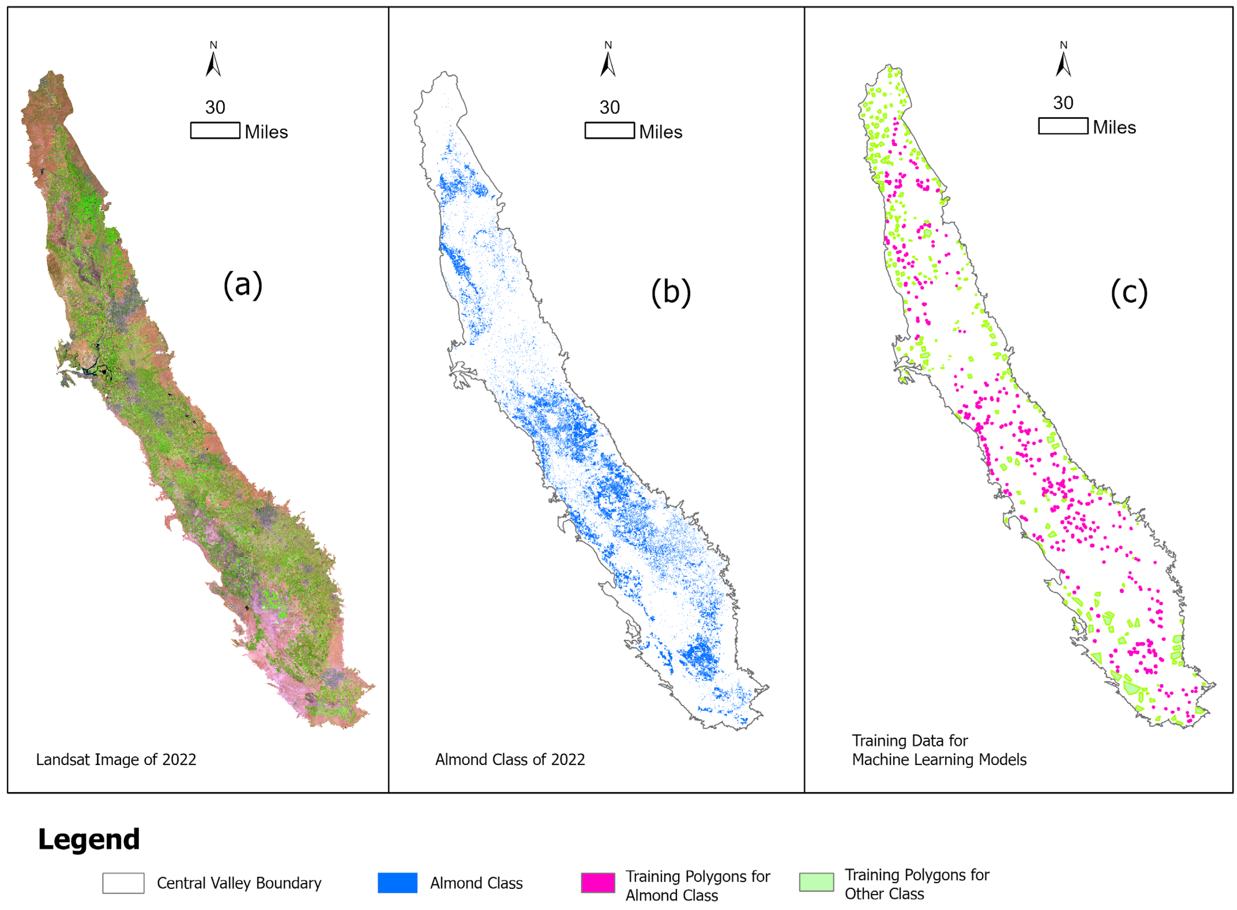
2.2.1. Satellite Image Data
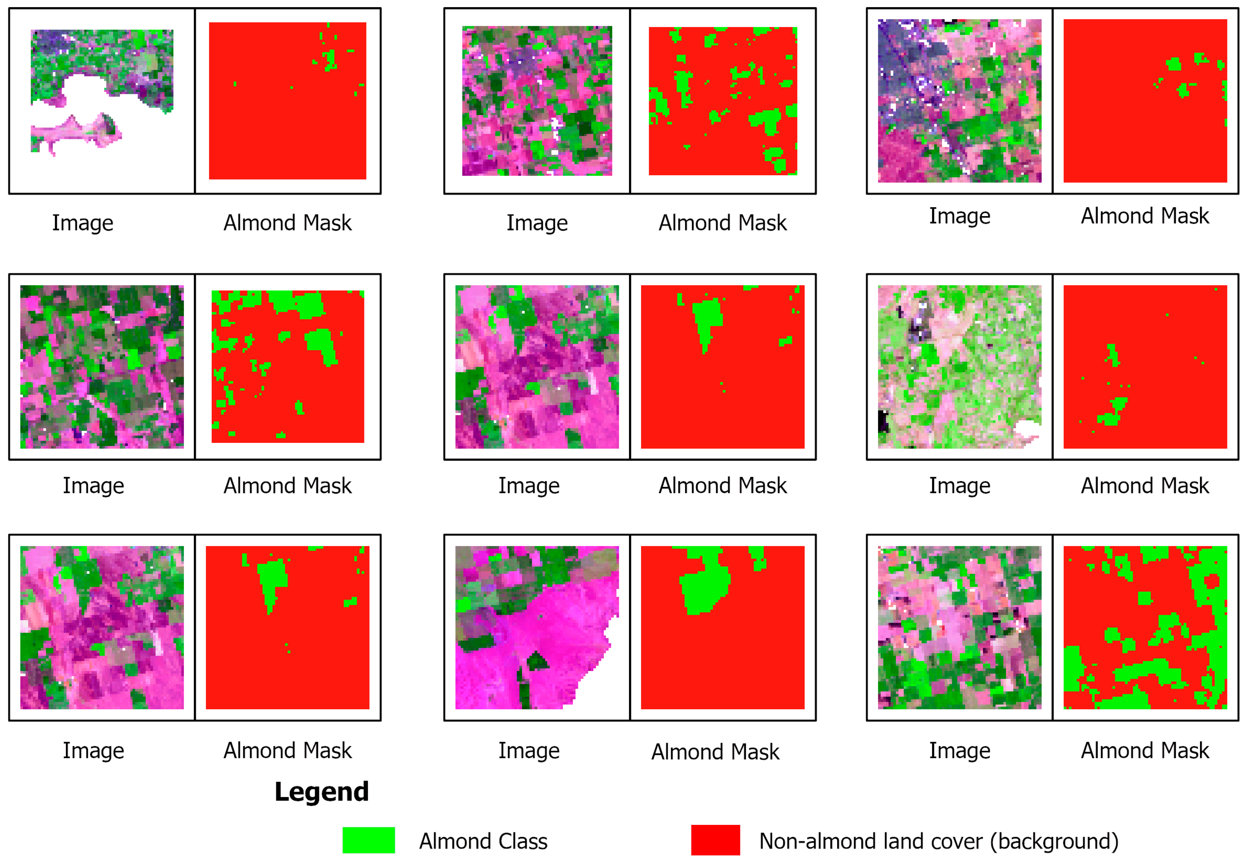
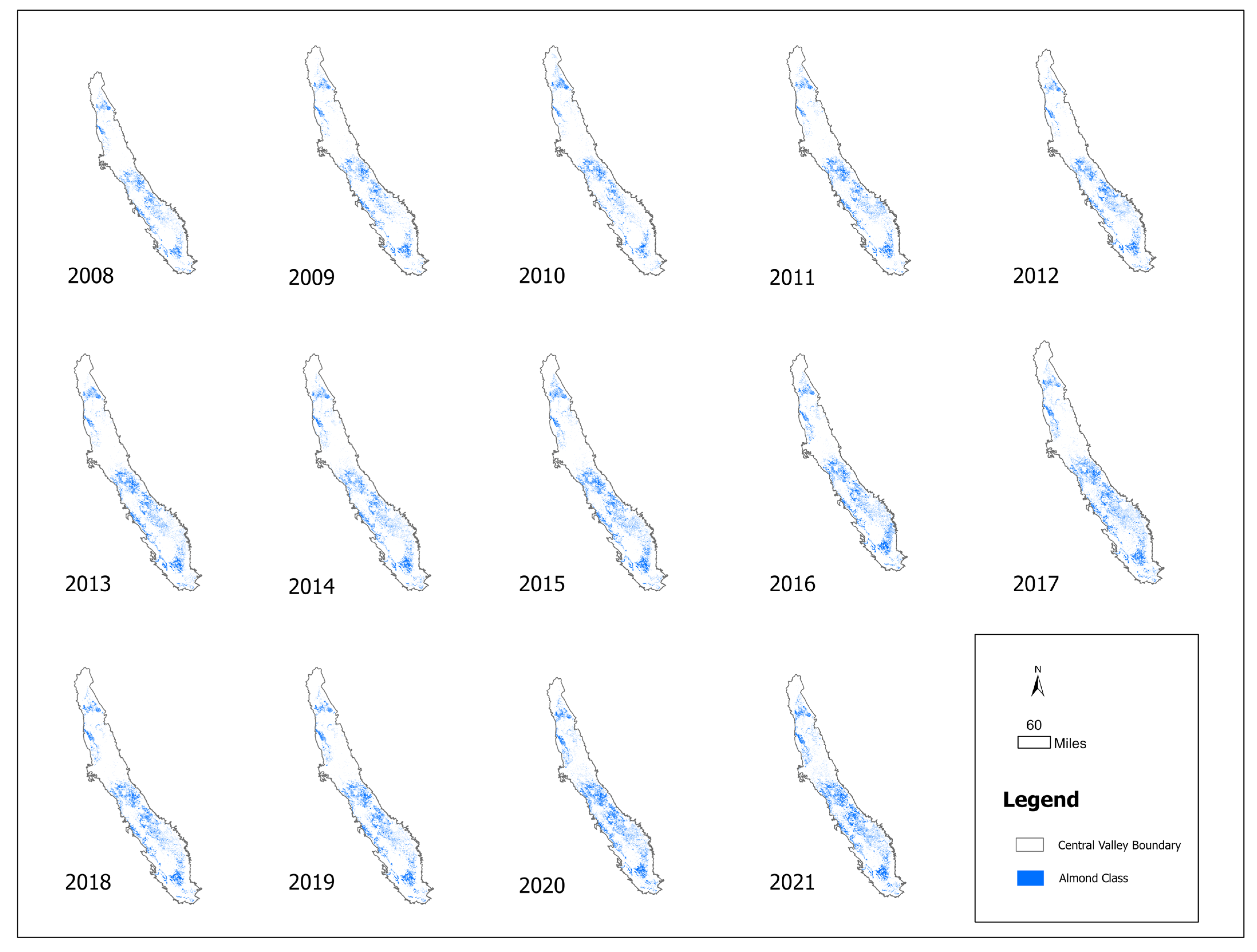
2.2.2. Crop Data for Almond Locations and Training
2.3. Model Selection and Setup
2.3.1. ML Models
2.3.2. DL Models
2.3.3. Computing Requirements for Analysis and Available Resources
2.3.4. Accuracy Assessment of ML and DL Models
3. Results
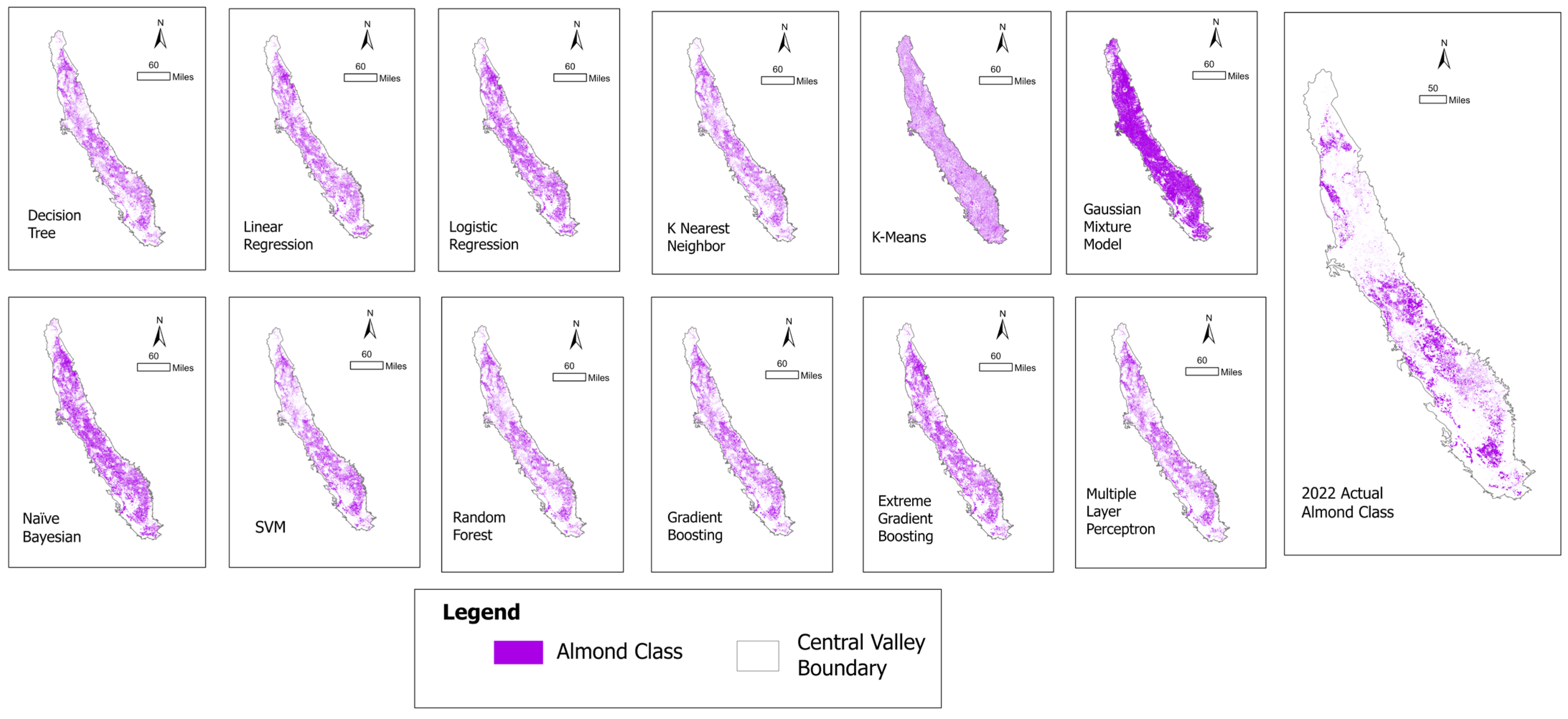
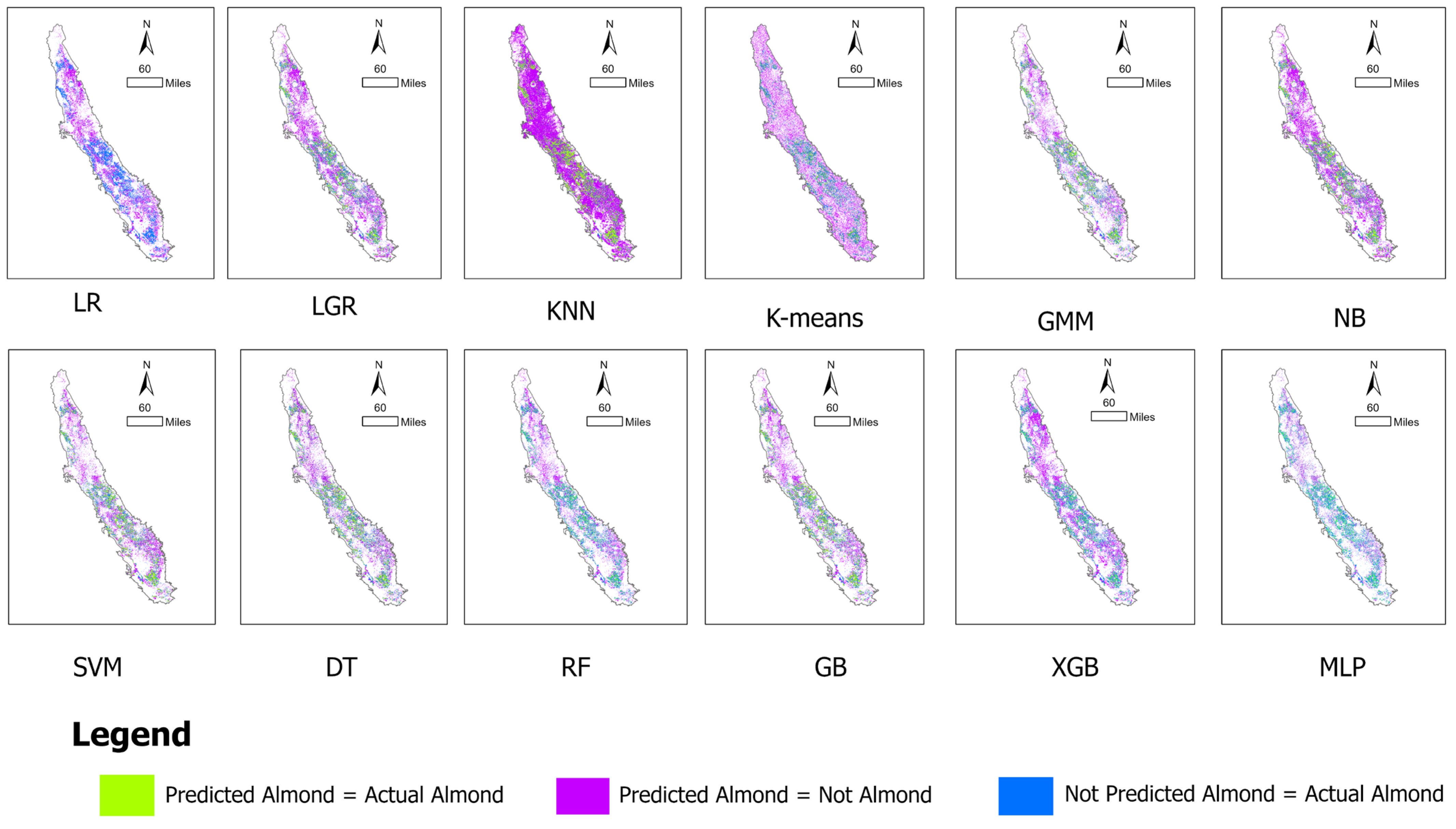
3.1. ML Model Performance
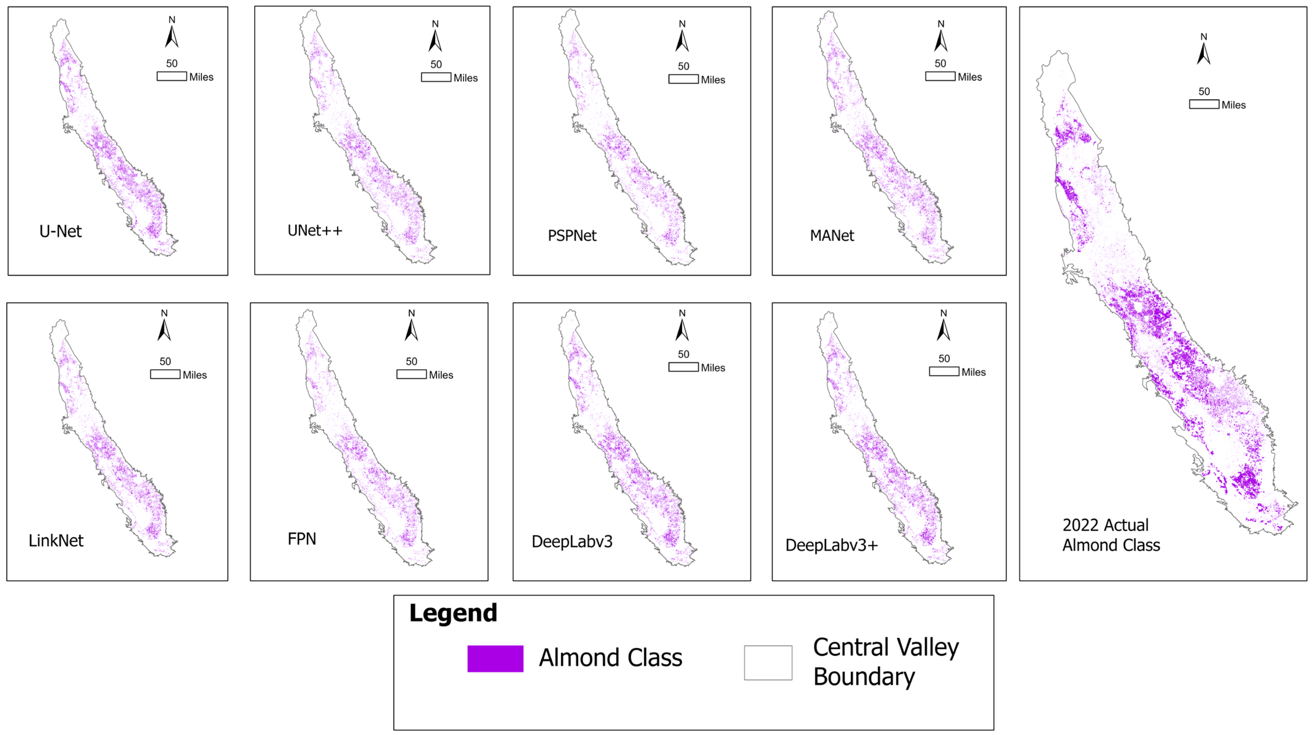
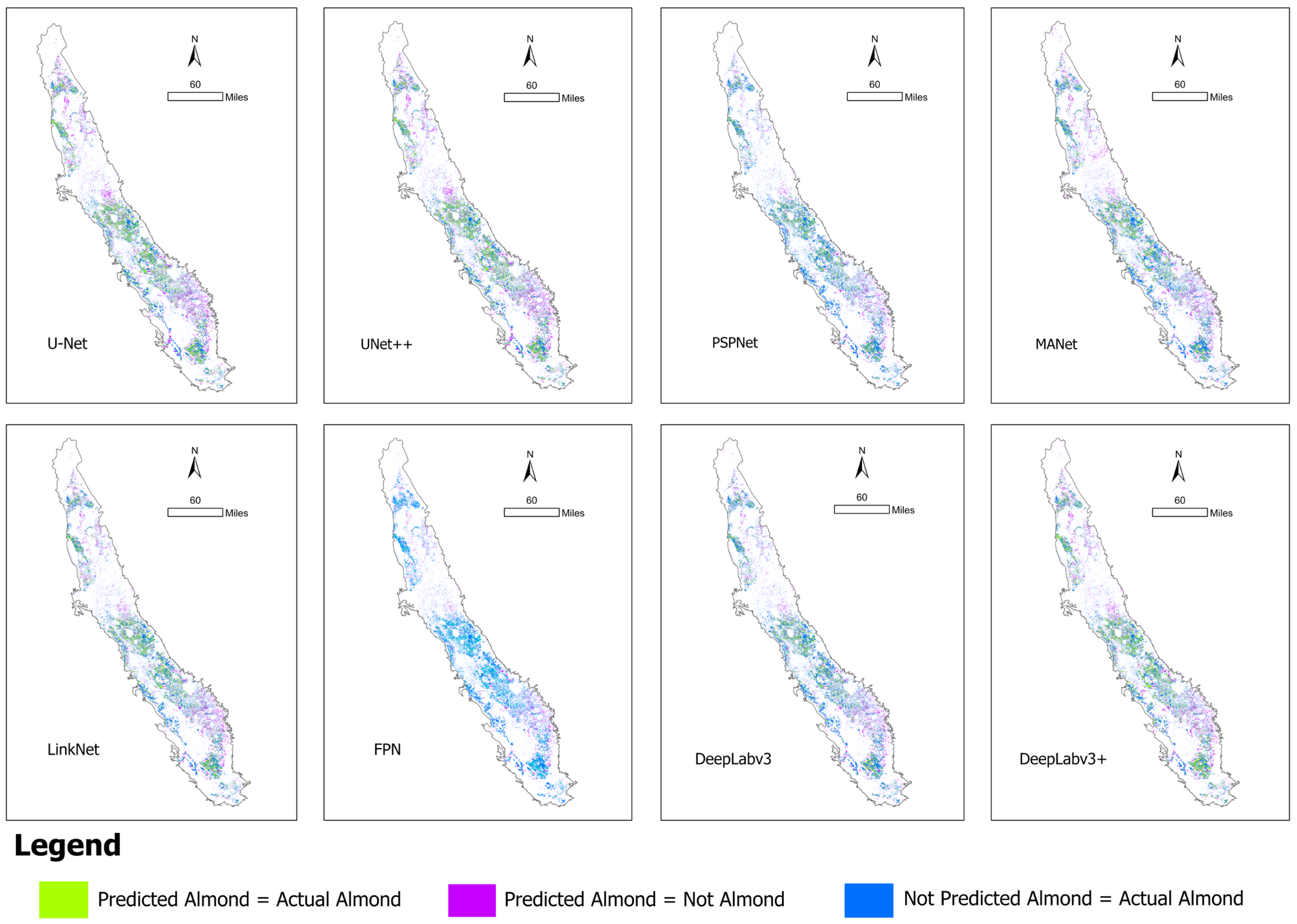
3.2. DL Model Performance
4. Discussion
5. Conclusions
Author Contributions
Funding
Data Availability Statement
Acknowledgments
Conflicts of Interest
References
- Singh, V. Agriculture and Food Resources. In Textbook of Environment and Ecology; Springer: Singapore, 2024; pp. 155–174. [Google Scholar] [CrossRef]
- Dethier, J.J.; Effenberger, A. Agriculture and development: A brief review of the literature. Econ. Syst. 2012, 36, 175–205. [Google Scholar] [CrossRef]
- Hultgren, A.; Carleton, T.; Delgado, M.; Gergel, D.R.; Greenstone, M.; Houser, T.; Hsiang, S.; Jina, A.; Kopp, R.E.; Malevich, S.B.; et al. Impacts of climate change on global agriculture accounting for adaptation. Nature 2025, 642, 644–652. [Google Scholar] [CrossRef] [PubMed]
- Lyu, H.; Xing, H.; Duan, T. Optimizing Water Resource Allocation for Food Security: An Evaluation of China’s Water Rights Trading Policy. Sustainability 2024, 16, 10443. [Google Scholar] [CrossRef]
- Farah, A.A.; Mohamed, M.A.; Musse, O.S.H.; Nor, B.A. The multifaceted impact of climate change on agricultural productivity: A systematic literature review of SCOPUS-indexed studies (2015–2024). Discov. Sustain. 2025, 6, 397. [Google Scholar] [CrossRef]
- Heesun, W. What Almond Growers Want This Year: Rain and Bees. 2016. Available online: https://www.cnbc.com/2016/01/26/prices-of-mighty-almonds-down-amid-el-nino-related-cold-rain.html (accessed on 21 July 2025).
- Faunt, C.C.; Belitz, K.; Hanson, R.T. Développement d’un modèle tridimensionnel de la texture sédimentaire des dépôts de remplissage de la Vallée Centrale, Californie, Etats-Unis. Hydrogeol. J. 2010, 18, 625–649. [Google Scholar] [CrossRef]
- Kocis, T.N.; Dahlke, H.E. Availability of high-magnitude streamflow for groundwater banking in the Central Valley, California. Environ. Res. Lett. 2017, 12, 084009. [Google Scholar] [CrossRef]
- Parker, L.E.; Abatzoglou, J.T. Shifts in the thermal niche of almond under climate change. Clim. Change 2018, 147, 211–224. [Google Scholar] [CrossRef]
- Liu, P.-W.; Famiglietti, J.S.; Purdy, A.J.; Adams, K.H.; McEvoy, A.L.; Reager, J.T.; Bindlish, R.; Wiese, D.N.; David, C.H.; Rodell, M. Groundwater depletion in California’s Central Valley accelerates during megadrought. Nat. Commun. 2022, 13, 7825. [Google Scholar] [CrossRef]
- Gebremichael, M.; Krishnamurthy, P.K.; Ghebremichael, L.T.; Alam, S. What drives crop land use change during multi-year droughts in California’s central valley? Prices or concern for water? Remote Sens. 2021, 13, 650. [Google Scholar] [CrossRef]
- Levy, Z.F.; Jurgens, B.C.; Burow, K.R.; Voss, S.A.; Faulkner, K.E.; Arroyo-Lopez, J.A.; Fram, M.S. Critical Aquifer Overdraft Accelerates Degradation of Groundwater Quality in California’s Central Valley during Drought. Geophys. Res. Lett. 2021, 48, e2021GL094398. [Google Scholar] [CrossRef]
- Faunt, C.C.; Traum, J.A.; Boyce, S.E.; Seymour, W.A.; Jachens, E.R.; Brandt, J.T.; Sneed, M.; Bond, S.; Marcelli, M.F. Groundwater Sustainability and Land Subsidence in California’s Central Valley. Water 2024, 16, 1189. [Google Scholar] [CrossRef]
- Lees, M.; Knight, R. Quantification of record-breaking subsidence in California’s San Joaquin Valley. Commun. Earth Environ. 2024, 5, 677. [Google Scholar] [CrossRef]
- Zhong, L.; Hu, L.; Zhou, H. Deep learning based multi-temporal crop classification. Remote Sens. Environ. 2019, 221, 430–443. [Google Scholar] [CrossRef]
- Atzberger, C. Advances in remote sensing of agriculture: Context description, existing operational monitoring systems and major information needs. Remote. Sens. 2013, 5, 949–981. [Google Scholar] [CrossRef]
- Veloso, A.; Mermoz, S.; Bouvet, A.; Le Toan, T.; Planells, M.; Dejoux, J.-F.; Ceschia, E. Understanding the temporal behavior of crops using Sentinel-1 and Sentinel-2-like data for agricultural applications. Remote Sens. Environ. 2017, 199, 415–426. [Google Scholar] [CrossRef]
- Wang, X.; Zhang, J.; Xun, L.; Wang, J.; Wu, Z.; Henchiri, M.; Zhang, S.; Zhang, S.; Bai, Y.; Yang, S.; et al. Evaluating the Effectiveness of Machine Learning and Deep Learning Models Combined Time-Series Satellite Data for Multiple Crop Types Classification over a Large-Scale Region. Remote Sens. 2022, 14, 2341. [Google Scholar] [CrossRef]
- Wulder, M.A.; Masek, J.G.; Cohen, W.B.; Loveland, T.R.; Woodcock, C.E. Opening the archive: How free data has enabled the science and monitoring promise of Landsat. Remote Sens. Environ. 2012, 122, 2–10. [Google Scholar] [CrossRef]
- Roy, D.P.; Wulder, M.A.; Loveland, T.R.; Woodcock, C.E.; Allen, R.G.; Anderson, M.C.; Helder, D.; Irons, J.R.; Johnson, D.M.; Kennedy, R.; et al. Landsat-8: Science and product vision for terrestrial global change research. Remote Sens. Environ. 2014, 145, 154–172. [Google Scholar] [CrossRef]
- Qu, C.; Li, P.; Zhang, C. A spectral index for winter wheat mapping using multi-temporal Landsat NDVI data of key growth stages. ISPRS J. Photogramm. Remote Sens. 2021, 175, 431–447. [Google Scholar] [CrossRef]
- Wei, L.; Yu, M.; Liang, Y.; Yuan, Z.; Huang, C.; Li, R.; Yu, Y. Precise crop classification using spectral-spatial-location fusion based on conditional random fields for UAV-borne hyperspectral remote sensing imagery. Remote Sens. 2019, 11, 2011. [Google Scholar] [CrossRef]
- Ahmed, M.; Mumtaz, R.; Anwar, Z.; Shaukat, A.; Arif, O.; Shafait, F. A Multi–Step Approach for Optically Active and Inactive Water Quality Parameter Estimation Using Deep Learning and Remote Sensing. Water 2022, 14, 2112. [Google Scholar] [CrossRef]
- Kavzoglu, T.; Colkesen, I. A kernel functions analysis for support vector machines for land cover classification. Int. J. Appl. Earth Obs. Geoinf. 2009, 11, 352–359. [Google Scholar] [CrossRef]
- Belgiu, M.; Drăgu, L. Random forest in remote sensing: A review of applications and future directions. ISPRS J. Photogramm. Remote Sens. 2016, 114, 24–31. [Google Scholar] [CrossRef]
- Noi, P.T.; Kappas, M. Comparison of Random Forest, k-Nearest Neighbor, and Support Vector Machine Classifiers for Land Cover Classification Using Sentinel-2 Imagery. Sensors 2017, 18, 18. [Google Scholar] [CrossRef]
- Wang, P.; Fan, E.; Wang, P. Comparative analysis of image classification algorithms based on traditional machine learning and deep learning. Pattern Recognit. Lett. 2021, 141, 61–67. [Google Scholar] [CrossRef]
- Bahrami, H.; Homayouni, S.; Safari, A.; Mirzaei, S.; Mahdianpari, M.; Reisi-Gahrouei, O. Deep learning-based estimation of crop biophysical parameters using multi-source and multi-temporal remote sensing observations. Agronomy 2021, 11, 1363. [Google Scholar] [CrossRef]
- Shirmard, H.; Farahbakhsh, E.; Müller, R.D.; Chandra, R. A review of machine learning in processing remote sensing data for mineral exploration. Remote. Sens. Environ. 2022, 268, 112750. [Google Scholar] [CrossRef]
- Zhu, L.; Huang, L.; Fan, L.; Huang, J.; Huang, F.; Chen, J.; Zhang, Z.; Wang, Y. Landslide susceptibility prediction modeling based on remote sensing and a novel deep learning algorithm of a cascade-parallel recurrent neural network. Sensors 2020, 20, 1576. [Google Scholar] [CrossRef]
- Ball, J.E.; Anderson, D.T.; Chan, C.S. Comprehensive survey of deep learning in remote sensing: Theories, tools, and challenges for the community. J. Appl. Remote Sens. 2017, 11, 042609. [Google Scholar] [CrossRef]
- Kussul, N.; Lavreniuk, M.; Skakun, S.; Shelestov, A. Deep Learning Classification of Land Cover and Crop Types Using Remote Sensing Data. IEEE Geosci. Remote Sens. Lett. 2017, 14, 778–782. [Google Scholar] [CrossRef]
- Maxwell, A.E.; Warner, T.A.; Fang, F. Implementation of machine-learning classification in remote sensing: An applied review. Int. J. Remote Sens. 2018, 39, 2784–2817. [Google Scholar] [CrossRef]
- Lary, D.J.; Alavi, A.H.; Gandomi, A.H.; Walker, A.L. Machine learning in geosciences and remote sensing. Geosci. Front. 2016, 7, 3–10. [Google Scholar] [CrossRef]
- Herckes, P.; Marcotte, A.R.; Wang, Y.; Collett, J.L. Fog composition in the Central Valley of California over three decades. Atmos. Res. 2015, 151, 20–30. [Google Scholar] [CrossRef]
- Faunt, C.C.; Sneed, M.; Traum, J.; Brandt, J.T. Water availability and land subsidence in the Central Valley, California, USA. Hydrogeol. J. 2016, 24, 675–684. [Google Scholar] [CrossRef]
- Schauer, M.; Senay, G.B. Characterizing crop water use dynamics in the Central Valley of California using Landsat-derived evapotranspiration. Remote Sens. 2019, 11, 1782. [Google Scholar] [CrossRef]
- Lo, M.H.; Famiglietti, J.S. Irrigation in California’s Central Valley strengthens the southwestern U.S. water cycle. Geophys. Res. Lett. 2013, 40, 301–306. [Google Scholar] [CrossRef]
- Aktas, T.; Thy, P.; Williams, R.B.; McCaffrey, Z.; Khatami, R.; Jenkins, B.M. Characterization of almond processing residues from the Central Valley of California for thermal conversion. Fuel Process. Technol. 2015, 140, 132–147. [Google Scholar] [CrossRef]
- Sun, J.; Di, L.; Sun, Z.; Shen, Y.; Lai, Z. County-level soybean yield prediction using deep CNN-LSTM model. Sensors 2019, 19, 4363. [Google Scholar] [CrossRef]
- Maulud, D.; Abdulazeez, A.M. A Review on Linear Regression Comprehensive in Machine Learning. J. Appl. Sci. Technol. Trends 2020, 1, 140–147. [Google Scholar] [CrossRef]
- Ray, S. A Quick Review of Machine Learning Algorithms. In Proceedings of the 2019 International Conference on Machine Learning, Big Data, Cloud and Parallel Computing (COMITCon), Faridabad, India, 14–16 February 2019; pp. 35–39. [Google Scholar]
- Akgun, A. A comparison of landslide susceptibility maps produced by logistic regression, multi-criteria decision, and likelihood ratio methods: A case study at İzmir, Turkey. Landslides 2012, 9, 93–106. [Google Scholar] [CrossRef]
- Boateng, E.Y.; Abaye, D.A. A Review of the Logistic Regression Model with Emphasis on Medical Research. J. Data Anal. Inf. Process. 2019, 07, 190–207. [Google Scholar] [CrossRef]
- Wickramasinghe, I.; Kalutarage, H. Naive Bayes: Applications, variations and vulnerabilities: A review of literature with code snippets for implementation. Soft Comput. 2021, 25, 2277–2293. [Google Scholar] [CrossRef]
- Jiang, L.; Zhang, L.; Li, C.; Wu, J. A Correlation-Based Feature Weighting Filter for Naive Bayes. IEEE Trans. Knowl. Data Eng. 2019, 31, 201–213. [Google Scholar] [CrossRef]
- Patle, A.; Chouhan, D.S. SVM kernel functions for classification. In Proceedings of the 2013 International Conference on Advances in Technology and Engineering (ICATE), Mumbai, India, 23–25 January 2013; pp. 1–9. [Google Scholar] [CrossRef]
- Sheykhmousa, M.; Mahdianpari, M.; Ghanbari, H.; Mohammadimanesh, F.; Ghamisi, P.; Homayouni, S. Support Vector Machine Versus Random Forest for Remote Sensing Image Classification: A Meta-Analysis and Systematic Review. IEEE J. Sel. Top. Appl. Earth Obs. Remote. Sens. 2020, 13, 6308–6325. [Google Scholar] [CrossRef]
- Abu Alfeilat, H.A.; Hassanat, A.B.; Lasassmeh, O.; Tarawneh, A.S.; Alhasanat, M.B.; Salman, H.S.E.; Prasath, V.S. Effects of Distance Measure Choice on K-Nearest Neighbor Classifier Performance: A Review. Big Data 2019, 7, 221–248. [Google Scholar] [CrossRef] [PubMed]
- Ali, I.; Rehman, A.U.; Khan, D.M.; Khan, Z.; Shafiq, M.; Choi, J.G. Model Selection Using K-Means Clustering Algorithm for the Symmetrical Segmentation of Remote Sensing Datasets. Symmetry 2022, 14, 1149. [Google Scholar] [CrossRef]
- Kawabata, T. Gaussian-input Gaussian mixture model for representing density maps and atomic models. J. Struct. Biol. 2018, 203, 1–16. [Google Scholar] [CrossRef]
- Myles, A.J.; Feudale, R.N.; Liu, Y.; Woody, N.A.; Brown, S.D. An introduction to decision tree modeling. J. Chemom. 2004, 18, 275–285. [Google Scholar] [CrossRef]
- Cutler, D.R.; Edwards, T.C., Jr.; Beard, K.H.; Cutler, A.; Hess, K.T.; Gibson, J.; Lawler, J.J. Random forests for classification in ecology. Ecology 2007, 88, 2783–2792. [Google Scholar] [CrossRef]
- Bentéjac, C.; Csörgő, A.; Martínez-Muñoz, G. A comparative analysis of gradient boosting algorithms. Artif. Intell. Rev. 2021, 54, 1937–1967. [Google Scholar] [CrossRef]
- Gupta, A.; Rajput, I.S.; Gunjan; Jain, V.; Chaurasia, S. NSGA-II-XGB: Meta-heuristic feature selection with XGBoost framework for diabetes prediction. Concurr. Comput. 2022, 34, e7123. [Google Scholar] [CrossRef]
- Cigizoglu, H.K. Estimation and forecasting of daily suspended sediment data by multi-layer perceptrons. Adv. Water Resour. 2004, 27, 185–195. [Google Scholar] [CrossRef]
- Su, Z.; Li, W.; Ma, Z.; Gao, R. An improved U-Net method for the semantic segmentation of remote sensing images. Appl. Intell. 2022, 52, 3276–3288. [Google Scholar] [CrossRef]
- Li, C.; Fu, L.; Zhu, Q.; Zhu, J.; Fang, Z.; Xie, Y.; Guo, Y.; Gong, Y. Attention enhanced u-net for building extraction from farmland based on google and worldview-2 remote sensing images. Remote Sens. 2021, 13, 4411. [Google Scholar] [CrossRef]
- Hoorali, F.; Khosravi, H.; Moradi, B. Automatic Bacillus anthracis bacteria detection and segmentation in microscopic images using UNet++. J. Microbiol. Methods 2020, 177, 106056. [Google Scholar] [CrossRef] [PubMed]
- Zhou, Z.; Siddiquee, M.M.R.; Tajbakhsh, N.; Liang, J. UNet++: Redesigning Skip Connections to Exploit Multiscale Features in Image Segmentation. IEEE Trans. Med. Imaging 2020, 39, 1856–1867. [Google Scholar] [CrossRef] [PubMed]
- Xu, Y.; Lam, H.K.; Jia, G. MANet: A two-stage deep learning method for classification of COVID-19 from Chest X-ray images. Neurocomputing 2021, 443, 96–105. [Google Scholar] [CrossRef]
- Chen, B.; Xia, M.; Qian, M.; Huang, J. MANet: A multi-level aggregation network for semantic segmentation of high-resolution remote sensing images. Int. J. Remote Sens. 2022, 43, 5874–5894. [Google Scholar] [CrossRef]
- Pravitasari, A.; Asnawi, M.; Nugraha, F.; Darmawan, G.; Hendrawati, T. Enhancing 3D Lung Infection Segmentation with 2D U-Shaped Deep Learning Variants. Appl. Sci. 2023, 13, 11640. [Google Scholar] [CrossRef]
- Zhang, Y.; Ding, F.; Kwong, S.; Zhu, G. Feature pyramid network for diffusion-based image inpainting detection. Inf. Sci. 2021, 572, 29–42. [Google Scholar] [CrossRef]
- Dhalla, S.; Maqbool, J.; Mann, T.S.; Gupta, A.; Mittal, A.; Aggarwal, P.; Saluja, K.; Kumar, M.; Saini, S.S. Semantic segmentation of palpebral conjunctiva using predefined deep neural architectures for anemia detection. Procedia Comput. Sci. 2023, 218, 328–337. [Google Scholar] [CrossRef]
- Shi, T.; Guo, Z.; Li, C.; Lan, X.; Gao, X.; Yan, X. Improvement of deep learning Method for water body segmentation of remote sensing images based on attention modules. Earth Sci. Inf. 2023, 16, 2865–2876. [Google Scholar] [CrossRef]
- Yin, Y.; Guo, Y.; Deng, L.; Chai, B. Improved PSPNet-based water shoreline detection in complex inland river scenarios. Complex. Intell. Syst. 2023, 9, 233–245. [Google Scholar] [CrossRef]
- Zhang, X.Y.; Rahman, A.H.A.; Qamar, F. Semantic visual simultaneous localization and mapping (SLAM) using deep learning for dynamic scenes. PeerJ Comput. Sci. 2023, 9, e1628. [Google Scholar] [CrossRef]
- Cai, C.; Tan, J.; Zhang, P.; Ye, Y.; Zhang, J. Determining Strawberries’ Varying Maturity Levels by Utilizing Image Segmentation Methods of Improved DeepLabV3+. Agronomy 2022, 12, 1875. [Google Scholar] [CrossRef]
- Abdulkareem, K.H.; Mohammed, M.A.; Gunasekaran, S.S.; Al-Mhiqani, M.N.; Mutlag, A.A.; Mostafa, S.A.; Ali, N.S.; Ibrahim, D.A. A review of fog computing and machine learning: Concepts, applications, challenges, and open issues. IEEE Access 2019, 7, 153123–153140. [Google Scholar] [CrossRef]
- Wang, X.; Huang, J.; Feng, Q.; Yin, D. Winter wheat yield prediction at county level and uncertainty analysis in main wheat-producing regions of China with deep learning approaches. Remote Sens. 2020, 12, 1744. [Google Scholar] [CrossRef]
- Nguyen, G.; Dlugolinsky, S.; Bobák, M.; Tran, V.; García, Á.L.; Heredia, I.; Malík, P.; Hluchý, L. Machine Learning and Deep Learning frameworks and libraries for large-scale data mining: A survey. Artif. Intell. Rev. 2019, 52, 77–124. [Google Scholar] [CrossRef]
- Mukhamediev, R.I.; Popova, Y.; Kuchin, Y.; Zaitseva, E.; Kalimoldayev, A.; Symagulov, A.; Levashenko, V.; Abdoldina, F.; Gopejenko, V.; Yakunin, K.; et al. Review of Artificial Intelligence and Machine Learning Technologies: Classification, Restrictions, Opportunities and Challenges. Mathematics 2022, 10, 2552. [Google Scholar] [CrossRef]
- Butt, U.A.; Mehmood, M.; Shah, S.B.H.; Amin, R.; Shaukat, M.W.; Raza, S.M.; Suh, D.Y.; Piran, J. A review of machine learning algorithms for cloud computing security. Electronics 2020, 9, 1379. [Google Scholar] [CrossRef]
- Gill, S.S.; Xu, M.; Ottaviani, C.; Patros, P.; Bahsoon, R.; Shaghaghi, A.; Golec, M.; Stankovski, V.; Wu, H.; Abraham, A.; et al. AI for next generation computing: Emerging trends and future directions. Internet Things 2022, 19, 100514. [Google Scholar] [CrossRef]
- Alsadie, D. A Comprehensive Review of AI Techniques for Resource Management in Fog Computing: Trends, Challenges, and Future Directions. IEEE Access 2024, 12, 118007–118059. [Google Scholar] [CrossRef]
- Hasan, A.S.M.M.; Diepeveen, D.; Laga, H.; Jones, M.G.; Sohel, F. Image patch-based deep learning approach for crop and weed recognition. Ecol. Inf. 2023, 78, 102361. [Google Scholar] [CrossRef]
- Streiner, D.L.; Norman, G.R. ‘Precision’ and ‘accuracy’: Two terms that are neither. J. Clin. Epidemiol. 2006, 59, 327–330. [Google Scholar] [CrossRef] [PubMed]
- Suji, R.J.; Godfrey, W.W.; Dhar, J. Exploring pretrained encoders for lung nodule segmentation task using LIDC-IDRI dataset. Multimed. Tools Appl. 2024, 83, 9685–9708. [Google Scholar] [CrossRef]
- Wardhani, N.W.S.; Rochayani, M.Y.; Iriany, A.; Sulistyono, A.D.; Lestantyo, P. Cross-validation Metrics for Evaluating Classification Performance on Imbalanced Data. In Proceedings of the 2019 International Conference on Computer, Control, Informatics and its Applications (IC3INA), Tangerang, Indonesia, 23–24 October 2019; pp. 14–18. [Google Scholar] [CrossRef]
- Ali, U.A.M.E.; Hossain, M.A. Feature Subspace Detection for Hyperspectral Images Classification using Segmented Principal Component Analysis and F-score. In Proceedings of the 2020 IEEE Region 10 Symposium (TENSYMP), Dhaka, Bangladesh, 5–7 June 2020; pp. 134–137. [Google Scholar] [CrossRef]
- Zhao, J.; Wang, X.; Dou, X.; Zhao, Y.; Fu, Z.; Guo, M.; Zhang, R. A high-precision image classification network model based on a voting mechanism. Int. J. Digit. Earth 2022, 15, 2168–2183. [Google Scholar] [CrossRef]
- Flint, L.E.; Flint, A.L.; Mendoza, J.; Kalansky, J.; Ralph, F.M. Characterizing drought in California: New drought indices and scenario-testing in support of resource management. Ecol. Process 2018, 7, 1. [Google Scholar] [CrossRef]
- Hanak, E.; Lund, J.R. Adapting California’s water management to climate change. Clim. Change 2012, 111, 17–44. [Google Scholar] [CrossRef]
- He, X.; Wada, Y.; Wanders, N.; Sheffield, J. Intensification of hydrological drought in California by human water management. Geophys. Res. Lett. 2017, 44, 1777–1785. [Google Scholar] [CrossRef]
- Melton, F.S.; Johnson, L.F.; Lund, C.P.; Pierce, L.L.; Michaelis, A.R.; Hiatt, S.H.; Guzman, A.; Adhikari, D.D.; Purdy, A.J.; Rosevelt, C.; et al. Satellite irrigation management support with the terrestrial observation and prediction system: A framework for integration of satellite and surface observations to support improvements in agricultural water resource management. IEEE J. Sel. Top. Appl. Earth Obs. Remote Sens. 2012, 5, 1709–1721. [Google Scholar] [CrossRef]
- Wilson, T.S.; Sleeter, B.M.; Cameron, D.R. Future land-use related water demand in California. Environ. Res. Lett. 2016, 11, 054018. [Google Scholar] [CrossRef]
- Cracknell, M.J.; Reading, A.M. Geological mapping using remote sensing data: A comparison of five machine learning algorithms, their response to variations in the spatial distribution of training data and the use of explicit spatial information. Comput. Geosci. 2014, 63, 22–33. [Google Scholar] [CrossRef]
- Hudait, M.; Patel, P.P. Crop-type mapping and acreage estimation in smallholding plots using Sentinel-2 images and machine learning algorithms: Some comparisons. Egypt. J. Remote Sens. Space Sci. 2022, 25, 147–156. [Google Scholar] [CrossRef]
- Wu, L.; Zhu, X.; Lawes, R.; Dunkerley, D.; Zhang, H. Comparison of machine learning algorithms for classification of LiDAR points for characterization of canola canopy structure. Int. J. Remote Sens. 2019, 40, 5973–5991. [Google Scholar] [CrossRef]
- Islam, N.; Rashid, M.; Wibowo, S.; Xu, C.-Y.; Morshed, A.; Wasimi, S.A.; Moore, S.; Rahman, S.M. Early weed detection using image processing and machine learning techniques in an australian chilli farm. Agriculture 2021, 11, 387. [Google Scholar] [CrossRef]
- Jwo, D.-J.; Chiu, S.-F. Deep learning based automated detection of diseases from apple leaf images. Comput. Mater. Contin. 2022, 71, 1849–1866. [Google Scholar] [CrossRef]
- Lamba, M.; Gigras, Y.; Dhull, A. Classification of plant diseases using machine and deep learning. Open Comput. Sci. 2021, 11, 491–508. [Google Scholar] [CrossRef]
- Feizizadeh, B.; Alajujeh, K.M.; Lakes, T.; Blaschke, T.; Omarzadeh, D. A comparison of the integrated fuzzy object-based deep learning approach and three machine learning techniques for land use/cover change monitoring and environmental impacts assessment. GIsci Remote Sens. 2021, 58, 1543–1570. [Google Scholar] [CrossRef]
- Kirola, M.; Singh, N.; Joshi, K.; Chaudhary, S.; Gupta, A. Plants Diseases Prediction Framework: A Image-Based System Using Deep Learning. In Proceedings of the 2022 IEEE World Conference on Applied Intelligence and Computing (AIC), Sonbhadra, India, 17–19 June 2022. [Google Scholar] [CrossRef]
- Sujatha, R.; Chatterjee, J.M.; Jhanjhi, N.Z.; Brohi, S.N. Performance of deep learning vs machine learning in plant leaf disease detection. Microprocess. Microsyst. 2021, 80, 103615. [Google Scholar] [CrossRef]
- Yao, J.; Wu, J.; Xiao, C.; Zhang, Z.; Li, J. The Classification Method Study of Crops Remote Sensing with Deep Learning, Machine Learning, and Google Earth Engine. Remote Sens. 2022, 14, 2758. [Google Scholar] [CrossRef]
- Gómez-Carmona, O.; Casado-Mansilla, D.; Kraemer, F.A.; López-de-Ipiña, D.; García-Zubia, J. Exploring the computational cost of machine learning at the edge for human-centric Internet of Things. Future Gener. Comput. Syst. 2020, 112, 670–683. [Google Scholar] [CrossRef]
- Southworth, J.; Smith, A.C.; Safaei, M.; Rahaman, M.; Alruzuq, A.; Tefera, B.B.; Muir, C.S.; Herrero, H.V. Machine learning versus deep learning in land system science: A decision-making framework for effective land classification. Front. Remote. Sens. 2024, 5, 1374862. [Google Scholar] [CrossRef]
- Dosovitskiy, A.; Beyer, L.; Kolesnikov, A.; Weissenborn, D.; Zhai, X.; Unterthiner, T.; Dehghani, M.; Minderer, M.; Heigold, G.; Gelly, S.; et al. An Image is Worth 16x16 Words: Transformers for Image Recognition at Scale. arXiv 2021, arXiv:2010.11929. [Google Scholar] [CrossRef]
- Liu, Z.; Lin, Y.; Cao, Y.; Hu, H.; Wei, Y.; Zhang, Z.; Lin, S.; Guo, B. Swin Transformer: Hierarchical Vision Transformer using Shifted Windows. In Proceedings of the 2021 IEEE/CVF International Conference on Computer Vision (ICCV), Montreal, QC, Canada, 10–17 October 2021; pp. 9992–10002. [Google Scholar] [CrossRef]
- Touvron, H.; Cord, M.; Douze, M.; Massa, F.; Sablayrolles, A.; Jégou, H. Training data-efficient image transformers & distillation through attention. arXiv 2021, arXiv:2012.12877. [Google Scholar] [CrossRef]
- Ganjirad, M.; Bagheri, H. Google Earth Engine-based mapping of land use and land cover for weather forecast models using Landsat 8 imagery. Ecol. Inf. 2024, 80, 102498. [Google Scholar] [CrossRef]
- Pande, C.B.; Srivastava, A.; Moharir, K.N.; Radwan, N.; Sidek, L.M.; Alshehri, F.; Pal, S.C.; Tolche, A.D.; Zhran, M. Characterizing land use/land cover change dynamics by an enhanced random forest machine learning model: A Google Earth Engine implementation. Environ. Sci. Eur. 2024, 36, 84. [Google Scholar] [CrossRef]
- Brown, C.F.; Brumby, S.P.; Guzder-Williams, B.; Birch, T.; Hyde, S.B.; Mazzariello, J.; Czerwinski, W.; Pasquarella, V.J.; Haertel, R.; Ilyushchenko, S.; et al. Dynamic World, Near real-time global 10 m land use land cover mapping. Sci. Data 2022, 9, 251. [Google Scholar] [CrossRef]
- Miller, L.; Pelletier, C.; Webb, G.I. Deep Learning for Satellite Image Time-Series Analysis: A review. IEEE Geosci. Remote Sens. Mag. 2024, 12, 81–124. [Google Scholar] [CrossRef]
- Qichi, Y.; Lihui, W.; Jinliang, H.; Linzhi, L.; Xiaodong, L.; Fei, X.; Yun, D.; Xue, Y.; Feng, L. A novel alpine land cover classification strategy based on a deep convolutional neural network and multi-source remote sensing data in Google Earth Engine. GIsci Remote Sens. 2023, 60, 2233756. [Google Scholar] [CrossRef]


| Satellite | Date | Bands Extracted—Bandnumber, Name, Wavelength & Resolution |
|---|---|---|
| Landsat 5 | 2008–2009 | Band 3 Visible Red (0.63–0.69 µm) 30 m Band 4 Near-Infrared (0.76–0.90 µm) 30 m Band 5 Near-Infrared (1.55–1.75 µm) 30 m |
| Landsat 7 | 2012 | Band 3 Red (0.63–0.69 µm) 30 m Band 4 Near-Infrared (0.77–0.90 µm) 30 m Band 5 Short-Wave Infrared (1.55–1.75 µm) 30 m |
| Landsat 8–9 | 2013–2022 | Band 2—Blue (0.45–0.51 µm) 30 m; Band 5—Near-Infrared (0.85–0.88 µm) 30 m; Band 6—SWIR1 (1.57–1.65 µm) 30 m |
| Models | Hyperparameters |
|---|---|
| Deep Learning (General Structure) | ENCODER = “resnet50” ENCODER_WEIGHTS = ‘imagenet’ CLASSES = [“Almond”] ACTIVATION = ‘sigmoid’ DEVICE = ‘cuda’ Epoch = 150 chip_size = 64, stride_x = 8, stride_y = 8, crop = 12, n_channels = 3 |
| Linear Regression (LR) | LinearRegression () |
| Logistic Regression (LGR) | LogisticRegression () |
| Decision Tree (DT) | DecisionTreeClassifier () |
| Gaussian Mixture Model (GMM) | GaussianMixture (n_components = 3) |
| Gradient Boosting (GB) | GradientBoostingClassifier (n_estimators = 100, learning_rate = 0.1, max_depth = 3) |
| K-Means Clustering (K-Means) | KMeans (n_clusters = 100) |
| K-Nearest Neighbors (KNN) | KNeighborsClassifier (n_neighbors = 3) |
| Multi-Layer Perceptron (MLP) | MLPClassifier (hidden_layer_sizes = (150, 100, 50), max_iter = 100, activation = ‘relu’, solver = ‘adam’) |
| Naive Bayes (NB) | MultinomialNB () |
| Support Vector Machine (SVM) | SVC (C = 1.0, kernel = ‘rbf’, gamma = ‘scale’) |
| Extreme Gradient Boosting (XGB) | params = { ‘max_depth’: 3, ‘learning_rate’: 0.1, ‘n_estimators’: 50 } XGBClassifier(** params, tree_method = ‘gpu_hist’, predictor = ‘gpu_predictor’, gpu_id = 1) |
| Random Forest (RF) | RandomForestClassifier (n_estimators = 500, oob_score = True, verbose = 1) |
| ML Model | Precision | Recall | F1-Score | Overall Accuracy |
|---|---|---|---|---|
| Linear Regression—LR | 0.63 | 0.66 | 0.65 | 95.647 |
| Logistic Regression—LGR | 0.65 | 0.72 | 0.68 | 95.546 |
| K-Nearest Neighbor—KNN | 0.70 | 0.72 | 0.71 | 96.662 |
| K-Means Clustering—K-Means | 0.59 | 0.67 | 0.62 | 94.145 |
| Gaussian Mixture Model—GMM | 0.62 | 0.90 | 0.67 | 92.209 |
| Naive Bayesian—NB | 0.65 | 0.77 | 0.69 | 95.264 |
| Support Vector Machine—SVM | 0.61 | 0.58 | 0.59 | 96.100 |
| Decision Tree—DT | 0.70 | 0.74 | 0.72 | 96.650 |
| Random Forest—RF | 0.71 | 0.73 | 0.72 | 96.798 |
| Gradient Boosting—GB | 0.70 | 0.74 | 0.72 | 96.615 |
| Extreme Gradient Boosting—XGB | 0.67 | 0.74 | 0.69 | 95.93 |
| Multiple Layer Perceptron—MLP | 0.70 | 0.73 | 0.71 | 96.632 |
| Year | Precision | Recall | F1-Score | Overall Accuracy |
|---|---|---|---|---|
| U-Net | 0.79 | 0.66 | 0.70 | 97.465 |
| UNet++ | 0.79 | 0.62 | 0.66 | 97.394 |
| MANet | 0.78 | 0.62 | 0.67 | 97.338 |
| LinkNet | 0.80 | 0.64 | 0.69 | 97.455 |
| FPN | 0.80 | 0.61 | 0.66 | 97.422 |
| PSPNet | 0.80 | 0.60 | 0.65 | 97.404 |
| DeepLabv3 | 0.79 | 0.62 | 0.66 | 97.380 |
| DeepLabv3+ | 0.80 | 0.66 | 0.70 | 97.502 |
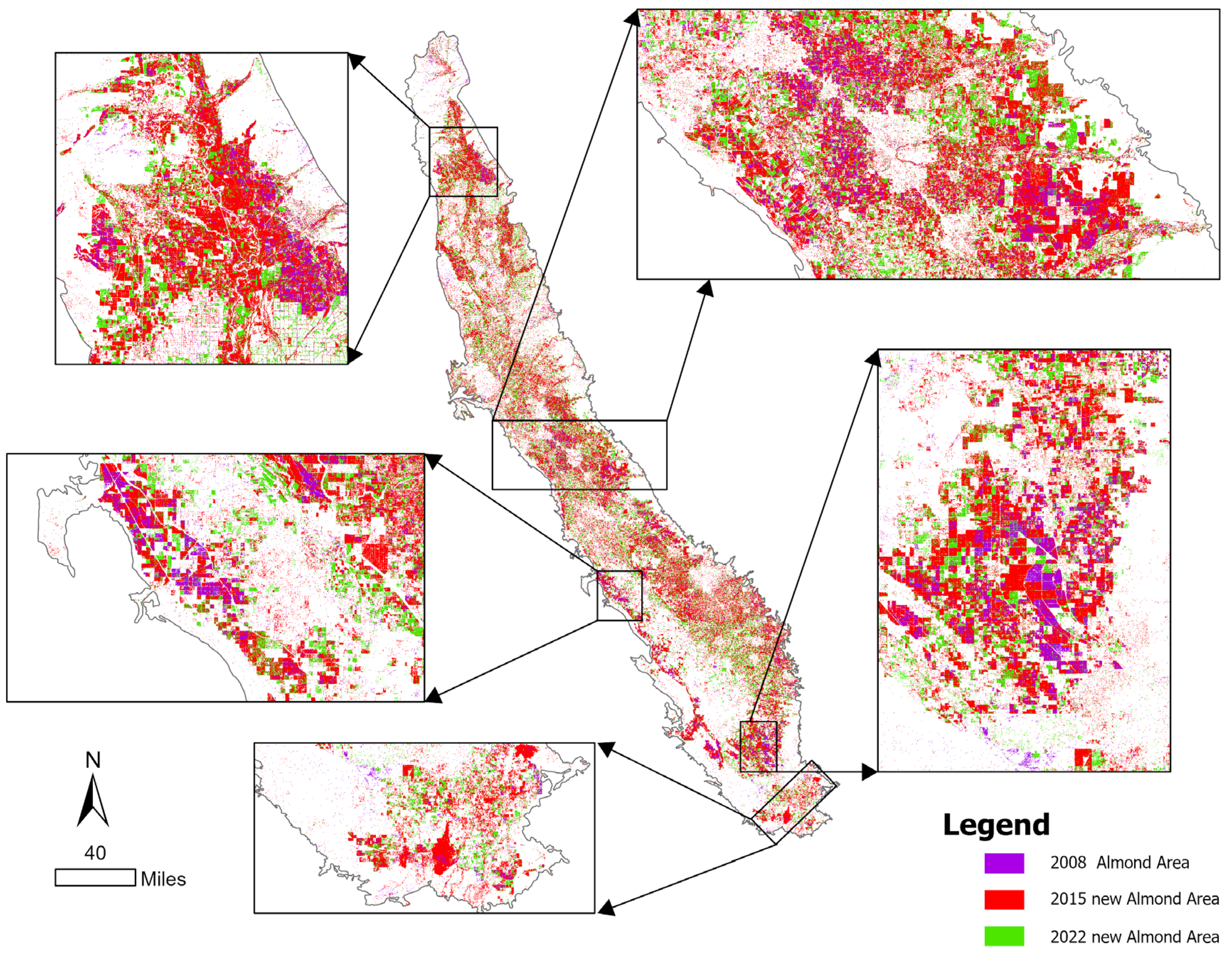
| Random Forest | Precision | Recall | F1-Score | Overall Accuracy |
|---|---|---|---|---|
| 2008 | 0.72 | 0.60 | 0.63 | 98.634 |
| 2015 | 0.69 | 0.80 | 0.73 | 97.158 |
| 2022 | 0.71 | 0.73 | 0.72 | 96.798 |
Disclaimer/Publisher’s Note: The statements, opinions and data contained in all publications are solely those of the individual author(s) and contributor(s) and not of MDPI and/or the editor(s). MDPI and/or the editor(s) disclaim responsibility for any injury to people or property resulting from any ideas, methods, instructions or products referred to in the content. |
© 2025 by the authors. Licensee MDPI, Basel, Switzerland. This article is an open access article distributed under the terms and conditions of the Creative Commons Attribution (CC BY) license (https://creativecommons.org/licenses/by/4.0/).
Share and Cite
Rahaman, M.; Southworth, J.; Wen, Y.; Keellings, D. Assessing Model Trade-Offs in Agricultural Remote Sensing: A Review of Machine Learning and Deep Learning Approaches Using Almond Crop Mapping. Remote Sens. 2025, 17, 2670. https://doi.org/10.3390/rs17152670
Rahaman M, Southworth J, Wen Y, Keellings D. Assessing Model Trade-Offs in Agricultural Remote Sensing: A Review of Machine Learning and Deep Learning Approaches Using Almond Crop Mapping. Remote Sensing. 2025; 17(15):2670. https://doi.org/10.3390/rs17152670
Chicago/Turabian StyleRahaman, Mashoukur, Jane Southworth, Yixin Wen, and David Keellings. 2025. "Assessing Model Trade-Offs in Agricultural Remote Sensing: A Review of Machine Learning and Deep Learning Approaches Using Almond Crop Mapping" Remote Sensing 17, no. 15: 2670. https://doi.org/10.3390/rs17152670
APA StyleRahaman, M., Southworth, J., Wen, Y., & Keellings, D. (2025). Assessing Model Trade-Offs in Agricultural Remote Sensing: A Review of Machine Learning and Deep Learning Approaches Using Almond Crop Mapping. Remote Sensing, 17(15), 2670. https://doi.org/10.3390/rs17152670