Study on Lithospheric Tectonic Features of Tianshan and Adjacent Regions and the Genesis Mechanism of the Wushi Ms7.1 Earthquake

Abstract

In this study, we analyzed the lithospheric seismic background of the Tianshan and adjacent areas by combining various geophysical methods (effective elastic thickness, time-varying gravity, apparent density, and InSAR), and explored the genesis mechanism of the Wushi Ms7.1 earthquake as an example, which led to the following conclusions: (1) The effective elastic thickness (Te) of the Tianshan lithosphere is low (13–28 km) and weak, while the Tarim and Junggar basins have Te > 30 km with high intensity, and the loads are all mainly from the surface (F < 0.5). Earthquakes occur mostly in areas with low values of Te. (2) Medium and strong earthquakes are prone to occur in regions with alternating positive and negative changes in the gravity field during the stage of large-scale reverse adjustment. It is expected that the risk of a moderate-to-strong earthquake occurring again in the vicinity of the survey area between 2025 and 2026 is relatively high. (3) Before the Wushi earthquake, the positive and negative boundaries of the apparent density of the crust at 12 km shifted to be approximately parallel to the seismic fault, and the earthquake was triggered after undergoing a “solidification” process. (4) The Wushi earthquake is a leptokurtic strike-slip backwash type of earthquake; coseismic deformation shows that subsidence occurs in the high-visual-density zone, and vice versa for uplift. The results of this study reveal the lithosphere-conceiving environment of the Tianshan and adjacent areas and provide a basis for regional earthquake monitoring, early warning, and post-disaster disposal.

1. Introduction

Earthquakes are among the natural disasters that threaten the safety of human lives and property, and more than 20 earthquakes of magnitude 8 or higher have occurred worldwide since the 21st century. These events have not only claimed the precious lives of many people but also caused incalculable damage to property. Our country is located between two major seismic belts—the Pacific Rim Seismic Belt and the Eurasian Seismic Belt—where strong earthquakes frequently occur. Previous researchers have conducted various studies on the background of earthquake generation, and some studies have found a relationship between lithosphere strength differences and the distribution of earthquakes [1,2,3]. So, many scholars, both at home and abroad, have researched the strength of the lithosphere [4,5,6], but research on the relationship between the earthquake-conceiving environment and the effective elastic thickness of the lithosphere remains insufficient, and the results of studies on Te values are still highly controversial. In addition, many scholars have found that the occurrence of earthquakes is associated with gravity [7,8,9], but most scholars still rely on gravity satellites for the acquisition of gravity data; gravity satellites are not able to detect small-scale features, and the revisit period is longer, so there is still a lack of research on the relationship between gravity and earthquakes.

The Ms7.1 earthquake occurred in January 2024 in Wushi, Xinjiang (78.66°E, 41.26°N), which is located in the Tianshan orogenic belt, an area of strong and frequent seismicity. In this region, the 1812 Nilgdong Ms8 earthquake, the 1902 Artux Ms8.2 earthquake, the 1906 Manas Ms7.7 earthquake, and the 1944 Wushi Ms7.2 earthquake all occurred. The Tianshan orogenic belt is one of the youngest and highest (>7000 m) orogenic belts in the world [10], and is the core component of the Central Asian giant orogenic system. It is a typical product of the Paleo-Asian ocean closure and landmass collage, which is characterized by both Paleoproterozoic collisional orogeny and Meso-Cenozoic intra-land reactivation. The Tianshan orogenic belt has a complex history, from the formation of the basement in the Paleozoic, through the Paleozoic ocean closure and collision, to the Cenozoic intraterrestrial reactivation [11]. Its evolution can be divided into several key stages, which involve multiple plate interactions, crustal shortening, and lithospheric deformation, and its tectonic features reflect the complete process from the Paleozoic ocean–land interaction to the Cenozoic intraterrestrial deformation [12], which has received extensive attention by domestic and foreign scholars [13,14,15,16,17]. Nowadays, the lithospheric tectonic activity in the region remains strong, but related research is not enough to summarize the patterns of earthquakes in the region. It is of great significance to continue in-depth research for the prevention and mitigation of earthquakes in the region.

Based on the above research status and background, this paper combines the effective elastic thickness of the lithosphere, gravity variations, and InSAR to study the background of earthquake generation in the Tianshan and neighboring areas. Firstly, using the lithospheric flexure isostasy model, the effective elastic thickness of the lithosphere in the Tianshan and adjacent areas was calculated using CRUST1.0 [18] topographic data and WGM2012 gravity anomaly data, based on the admittance and coherence joint inversion of Fan wavelet spectra. The integrated mechanical strength of the lithosphere was also analyzed, as well as its connection to earthquakes. Then, based on the 2017–2025 mobile gravity observations, the one-year scale gravity field changes were extracted via leveling, and field source apparent density was inverted using the equivalent source model [19] to analyze the changes in the gravity field and field source apparent density before and after the earthquake. The coseismic deformation field of the January 2024 Ms 7.1 Wushi earthquake was also inverted based on differential interferometric SAR (D-InSAR) using Sentinel-1 radar image data, and the deformation field was analyzed by inverting the fault slip model of the originating fault using the steepest descent method (SDM) program [20], which combines the deformation field with the effective elastic thickness and apparent density. The results of this study can complement research on the earthquake-conceiving environment in the Tianshan Mountains and neighboring areas and provide a reference for earthquake monitoring and early warning.

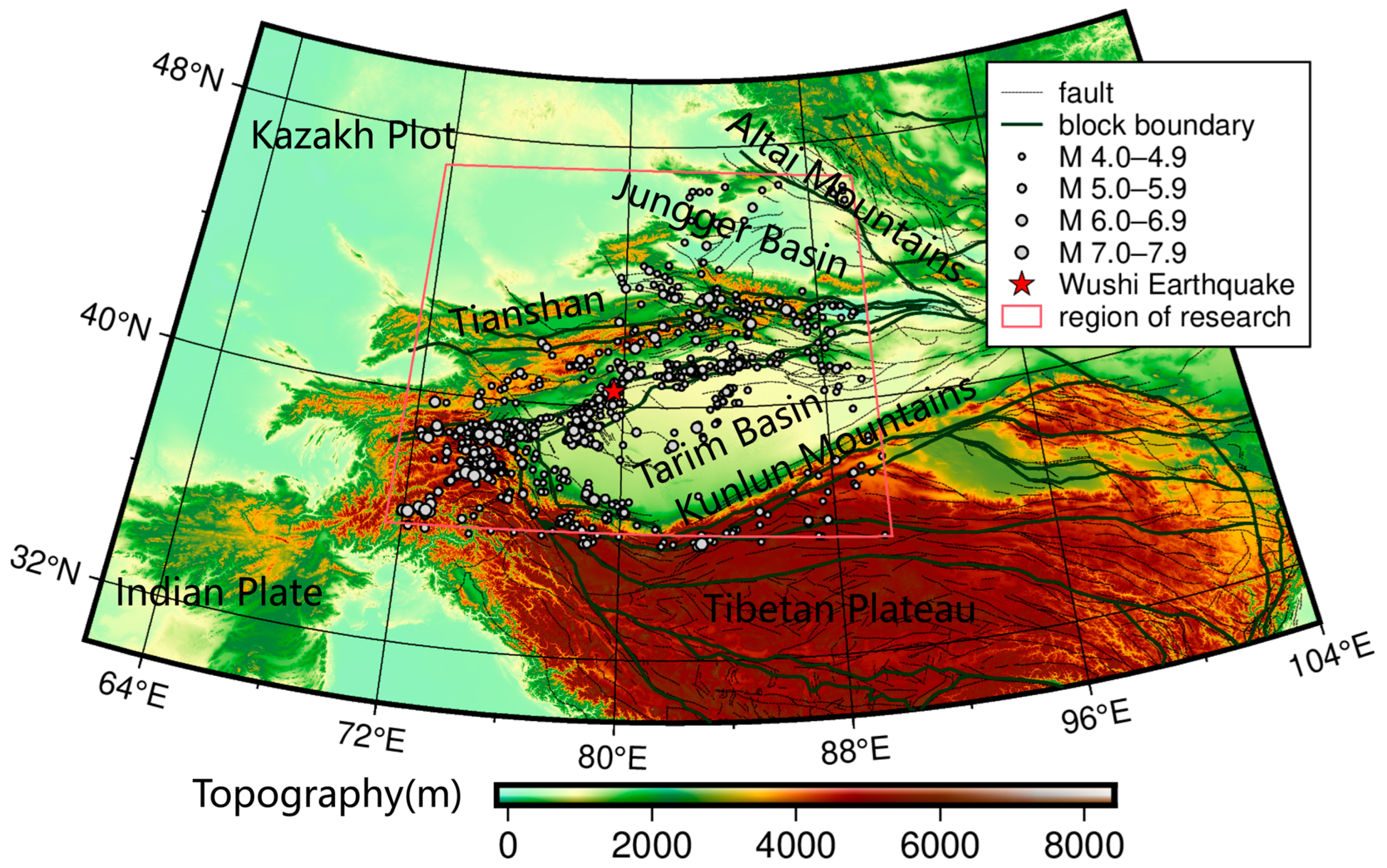
2. Geotectonic Background

Located in the hinterland of the Eurasian continent, the Tianshan is the world’s largest independent latitudinal mountain system and the farthest mountain system from the sea, spanning China, Kazakhstan, Kyrgyzstan, and Uzbekistan, with a total length of 2500 km. Together with the Altai Mountains and the Junggar Basin to the north, and the Tarim Basin and the Kunlun Mountains to the south, it forms a unique tectonic pattern of “three mountains and two basins” in the northwestern part of China (Figure 1).

Despite being thousands of kilometers away from the collision boundary between the Indian and Eurasian plates (the Himalayan orogenic belt), it is still subject to remote stress transfer in the lithosphere [21]. Since the Oligocene (~30 Ma), the continuous northward extrusion transfer of the Indian Plate has led to the subduction of the Tarim Massif and the Junggar Massif under the Tianshan Mountains, which has reactivated this ancient orogenic belt and manifested itself in rapid uplift, retrograde thrusting, and enhanced seismicity, resulting in the present-day active intraterrestrial orogenic belt. The Indian plate is currently extruding northward at about 50 mm·a⁻¹, while the Tianshan orogenic belt accommodates 44% of the present-day crustal shortening between India and Siberia [1]. The continuous extrusion has created an active state of faults, such as the Maidan Fault, which has experienced many earthquakes of magnitude 6 or higher in history, is characterized by retrograde, left-rotating strike-slip motion, and serves as the main boundary fault for the northward subduction of the Tarim Massif under the Tianshan Massif; the disordered thrusting system consisting of the Maidan and Keping Faults, with a deep slip surface controlling the northward subduction of the Tarim and modulating regional stresses, which once triggered the 1974 Aksu Ms7.3 earthquake; and the Nalati Fault, which triggered the 1902 Atushi Ms8.3 earthquake (the largest earthquake of its magnitude ever recorded in the Tianshan Mountains) and formed a surface rupture of more than 200 km.

The main body of the North Tianshan is a Late Paleozoic island arc and accretionary wedge, characterized by the presence of ophiolite suites and Carboniferous volcanic rocks [22]. Geochemical characteristics indicate that it formed in a post-arc extensional environment associated with southward subduction of the Paleo-North Tianshan Ocean [23,24]. It entered the tectonic quiet period in the Mesozoic, depositing Jurassic coal-bearing clastic rocks, and was resurrected by extrusion in the Cenozoic, with the development of the Western Conglomerate and a multi-phase flooding fan in front of the mountain [25]. As the tectonic hub of the Tianshan Mountains, the Middle Tianshan is centered on a Precambrian basement that includes the Paleoproterozoic Xingxingxia Group and the Paleoproterozoic Tianhu Group. The north and south boundaries are controlled by large shear zones, with the Azikuduk Fault on the northern margin and the Nalati Fault, characterized by left-rotating retrograde motion, on the southern margin, with a strike-slip rate of 2.5 mm·a⁻¹ [26]. The premontane zone on the south side of the Tianshan Mountains contains a number of dorsally folded mountain ranges with nearly east–west orientations. The row near the Tianshan Mountains consists of Triassic and Jurassic dorsally folded mountain ranges; the second row consists of Cretaceous as well as Lower Tertiary sandstones and mudstones; and the third row consists of sandstone conglomerates, mudstones, and Lower Pleistocene conglomerates.

3. Effective Elastic Thickness

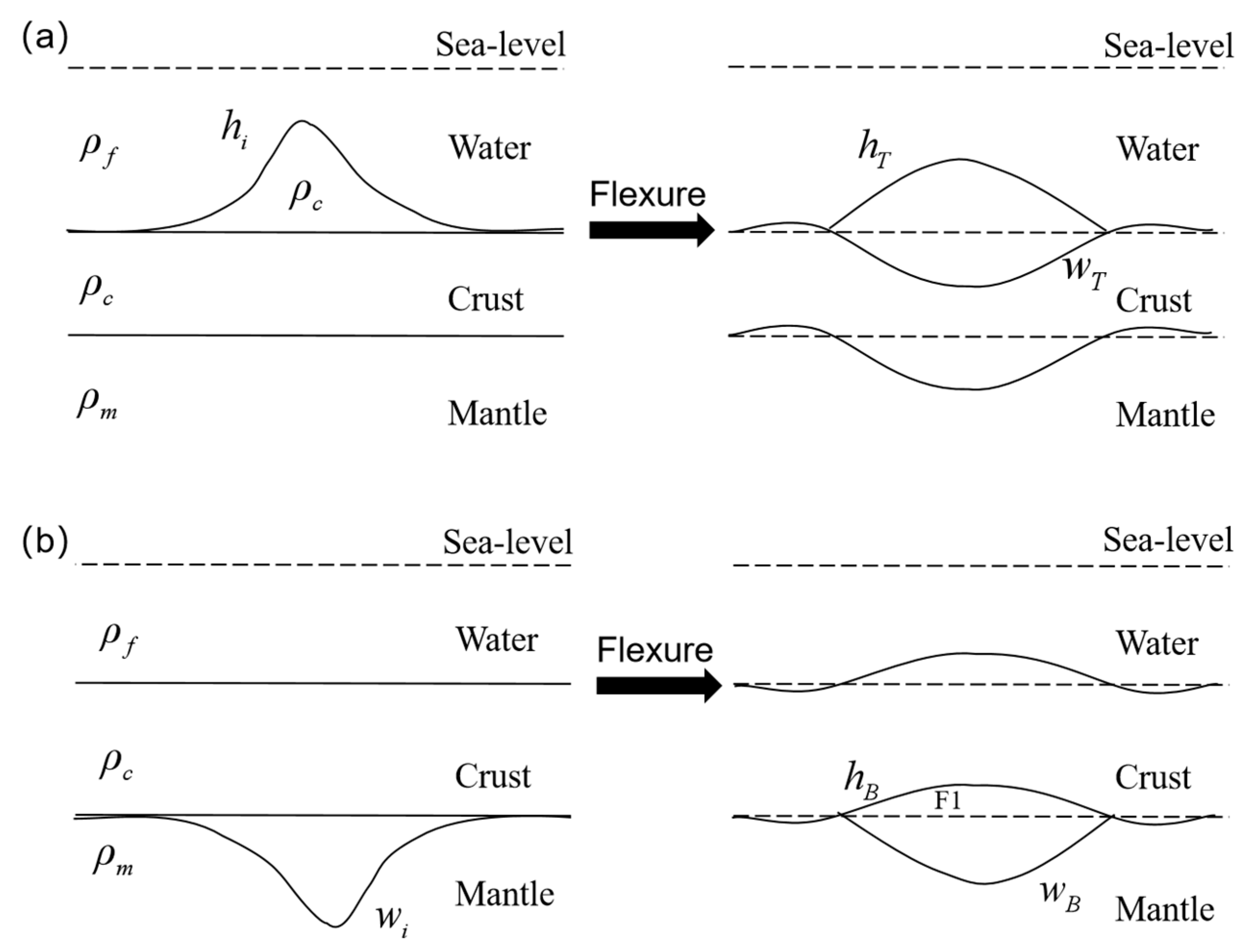
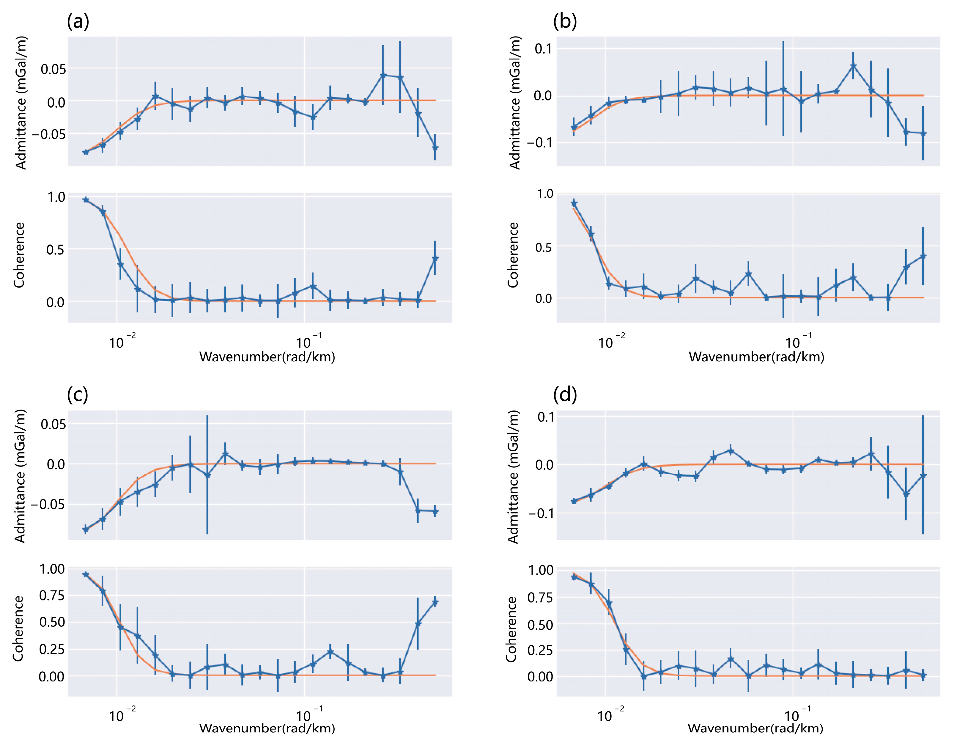
3.1. Methods and Principles

The lithospheric flexure isostasy model treats the lithosphere as an elastic sheet floating on top of the soft flow ring, and various topographic loads are applied to the elastic sheet, causing the sheet to undergo flexural deformation, a process that can be expressed by the elastic sheet flexural response equation:

$$D{\displaystyle \frac{{\partial }^{4}w}{\partial x^4}}+({\rho }_m-{\rho }_c)gw={\rho }_{\mathit{load}}{\mathit{gh}}_{\mathit{load}}$$

(1)

where $w$ denotes the deformation of the sheet during the flexural response; $x$ denotes the horizontal coordinate; ${\rho }_m$ and ${\rho }_c$ denote the fluid densities of the mantle and crust, respectively; $g$ denotes the acceleration of gravity; ${\rho }_{load}$ and $h_{load}$ denote the density and the height of the load, respectively; and $D$ denotes the flexural stiffness of the sheet. $D$ satisfies the proportionality relationship with T_e as follows:

$$D={\displaystyle \frac{E{T}_e^3}{12(1-v^2)}}$$

(2)

where $E$ denotes Young’s modulus, which takes the value of 1 × 10¹¹ N·M⁻²; and $v$ denotes Poisson’s ratio, which takes the value of 0.25. The loads are subdivided into surface loads and subsurface loads (Figure 2). When the equilibrium state is reached under surface loads, the following applies:

$$D{\displaystyle \frac{{\partial }^4{w}_T}{\partial x^4}}+({\rho }_m-{\rho }_c)g{w}_T=-({\rho }_c-{\rho }_f)g{h}_T$$

(3)

where $w_T$ denotes the deflection deformation formed under surface loads; $h_T$ denotes the surface deformation after the surface loads equalize the deflection; ${\rho }_f$ denotes the fluid density at the surface.

Real lithospheric loads are usually periodic in nature. After approximating the loads as periodic loads, Equation (3) will be expressed as follows:

$$W_T={\displaystyle \frac{-({\rho }_c-{\rho }_f)g{h}_T\cos (kx)}{({\rho }_m-{\rho }_c)}}{[{\displaystyle \frac{D{k}^4}{({\rho }_m-{\rho }_c)g}}+1]}^{-1}$$

(4)

where the negative sign indicates that the flexural deformation is negative for loads in the positive direction. The right end “[ ]”is defined as the flexural response function, as follows:

$${\Phi }_e(k)={[{\displaystyle \frac{D{k}^4}{({\rho }_{\mathrm{m}}-{\rho }_c)g}}+1]}^{-1}$$

(5)

Similarly, the deflection response function for the subsurface load is as follows:

$${{\Phi }^{\prime }}_e(k)={[{\displaystyle \frac{D{k}^4}{({\rho }_c-{\rho }_f)g}}+1]}^{-1}$$

(6)

However, for the actual Earth, it is very difficult to observe lithospheric deflection directly from the surface. Gravity anomalies, on the other hand, are sensitive to changes in load deflection and are easy to observe. At the same time, changes in topography will also cause changes in gravity, so deflection changes can be analyzed using gravity and topography. Considering the lithosphere as a kind of filter, topography serves as the input data, and the gravity anomaly caused by the deflection is the output data. Gravity conductivity is introduced to represent this filtering effect and to obtain the measured conductivity [28]:

$$Q_{obs}(k)={\displaystyle \frac{〈G(k)H^{*}(k)〉}{〈H(k)H^{*}(k)〉}}$$

(7)

where “$\langle \rangle$” denotes the average wave number, “ * ” denotes the complex conjugate, $k$ denotes the two-dimensional wave number, $k=\left|k\right|=\sqrt{k_x^2+k_y^2}$, $G(k)$ denotes the gravity anomaly spectrum in the wave number domain, and $H(k)$ denotes the topographic spectrum in the wave number domain. The observed correlation, derived from cross and auto-power spectra of topography and Bouguer gravity anomalies, reflects the consistency between topographic loading and lithospheric flexural response [29]:

$${\gamma }_{obs}^2(k)={\displaystyle \frac{{\left|〈G(k)H^{*}(k)〉\right|}^2}{〈G(k)G^{*}(k)〉〈H(k)H^{*}(k)〉}}$$

(8)

Based on Parker’s bit-field theory [30], we derive theoretical expressions for the admittance and coherence functions as follows [31]:

$$Q_{pre}(k)={\displaystyle \frac{{\mu }_T{k}_T+{\mu }_B{k}_B{f}^2{r}^2}{k_T^2+k_B^2{f}^2{r}^2}},r_{pre}^2(k)={\displaystyle \frac{{\left({\mu }_T{k}_T+{\mu }_B{k}_B{f}^2{r}^2\right)}^2}{\left({\mu }_T^2+{\mu }_B^2{f}^2{r}^2\right)\left(k_T^2+k_B^2{f}^2{r}^2\right)}}$$

(9)

where ${\mu }_B$ and ${\mu }_B$ are the gravitational inverse fold accumulation coefficients, $\phi =D{k}^4/g+{\rho }_m-{\rho }_f$, $\Delta {\rho }_1={\rho }_c-{\rho }_f$, $\mathrm{\Delta }{\rho }_2={\rho }_m-{\rho }_c$, $r=\mathrm{\Delta }{\rho }_1/\mathrm{\Delta }{\rho }_2$, $k_T=1-\mathrm{\Delta }{\rho }_1/\phi$, $k_B=-\mathrm{\Delta }{\rho }_2/\phi$, where $f$ denotes the ratio of the initial subsurface load to the amplitude of the surface load obtained to describe the initial load.

$$f^2={\displaystyle \frac{1}{r^2}}{\displaystyle \frac{〈{\left|w_i\right|}^2〉}{〈{\left|h_i\right|}^2〉}}$$

(10)

$h_i$, $w_i$ denote the amplitudes of the initial surface load and initial subsurface load, respectively. As later normalized by McKenzie, the load case is described by the variable $f$, called the load ratio:

$$F={\displaystyle \frac{f}{1+f}}$$

(11)

When only surface loads are present, $f=F=0$; when only subsurface loads are present, $f=F=0$; when surface and subsurface loads are the same, $f=1$, $F=0.5$.

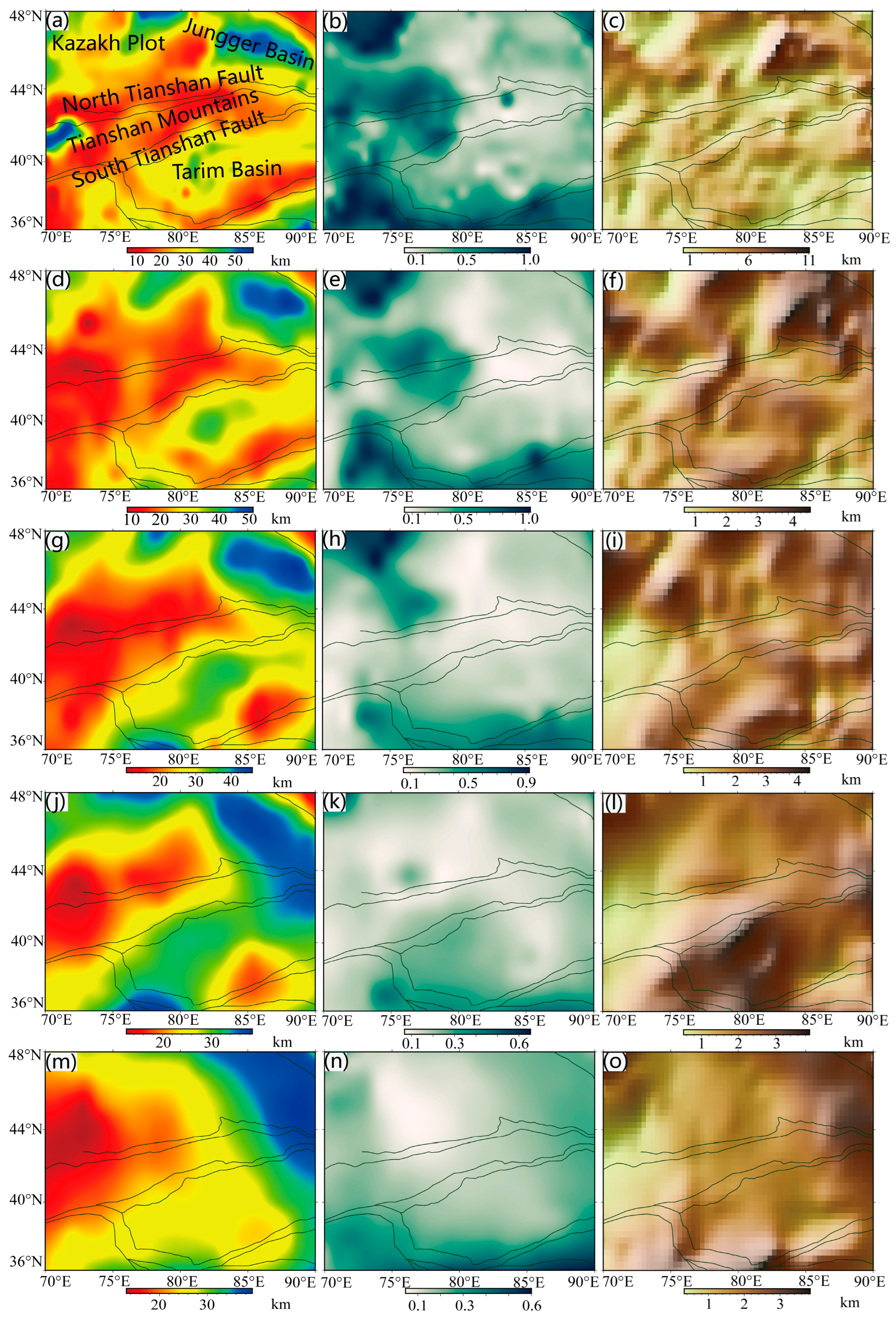
3.2. Data and Calculations

The topographic data, crustal data (crustal density and crustal thickness), and gravity anomaly data used to calculate Te in this paper are from ETOPO1, published by the National Geophysical Data Center (NGDC) and the National Oceanic and Atmospheric Administration (NOAA), respectively; CRUST1.0, released by the Institute of Geophysics and Planetary Physics (IGPP); and WGM2012, released by the Bureau Gravimetric International (BGI) [32]. These datasets have spatial resolutions of 1′ × 1′, 1° × 1°, and 2′ × 2′, respectively. The accuracy of the gravity field of WGM2012 in the terrestrial region is ±1–2 mGal, which is in accordance with the computational requirements in the field of solid-state geophysics [33,34].

In order to avoid the influence generated by boundary effects during the spectral calculation process, the actual range of data processed in this paper is larger than the study area, which also ensures that the calculation results have sufficient spatial resolution. In order to avoid the influence of the curvature of the Earth, all data are transformed from the geographic coordinate system to the Cartesian coordinate system using the Mercator projection. The joint inversion of the measured conductivity and the measured correlation is performed for each grid to calculate the effective elastic thickness Te and the load ratio F. The inversion process is based on the GEOIST (https://gitee.com/cea2020/geoist, accessed on 28 July 2025) open-source Python software package.

Through previous research on the wavelet spectral method, it is known that the selection of the center wave number has a large impact on the calculation results. A small center wave number $\left|k_0\right|$ provides finer inversion with higher spatial resolution, but increases the uncertainty of the inversion. A large center wave number makes the transition of the calculation results smoother and is more effective at calculating Te and F values in a larger region, but the resolution is reduced [35,36]. In this paper, we use $\left|k_0\right|$ = 2.668, 3.081, 3.773, 5.336, and 7.547 [35] to invert Te and F and calculate the Te fitting difference between the joint inversion of the measured conductivity–correlation function and the predicted conductivity–correlation, respectively. As can be seen in Figure 3, the results calculated using $\left|k_0\right|$ = 2.668, 3.081, and 3.773 have a high resolution, but the fitting difference is large. When using $\left|k_0\right|$ = 7.547, although the fitting difference is the smallest, the transition of the calculation result is too smooth, the calculation is rougher, and the resolution is lower. Therefore, to achieve higher spatial resolution and a smaller fitting difference, this paper selects the result of $\left|k_0\right|$ = 5.336 for subsequent discussion.

As can be seen from Figure 4, the Te values in the study area range from 13 to 39 km, with the highest Te value in the Junggar Basin, which is greater than 35 km. Overall, the lithospheric strength of the west side is slightly lower than that of the east side. Shi et al. [37] used the joint inversion method of the conductivity and correlation function along with the Bayesian optimal parameter estimation method to calculate the Te value of 20–40 km. Liu et al. [38] calculated a Te value of 5–50 km. These results are similar to the results of this paper, and all exhibit a west-low–east-high distribution pattern. As seen in Figure 4, the standard deviation of Te is less than 4 km, and most values are within 2 km. This demonstrates the accuracy of the calculation results in this paper. In addition, this paper also randomly selected several grid cells to analyze their measured conductivity and predicted conductivity, as well as the measured correlation and predicted correlation of the fit. As shown by the fitting curve in Figure 5, the degree of agreement between the measured and predicted values is generally better, which confirms the reliability of the conductivity–correlation function used in the joint inversion method in this paper.

For each landmass, the lowest Te value is located in the western foothills of the Tianshan Mountains, at less than 18 km. Plate extrusion has led to the continuous shortening of the Tianshan crust, and the rate of shortening decreases from west to east. Thus, the Te value of the western foothills of the Tianshan Mountains to the eastern foothills of the Tianshan Mountains shows an increasing trend. However, the overall Te value of Tianshan is low, and the lithosphere is fragile, which also leads to the frequent occurrence of earthquakes. The Te value of the Tarim Basin is relatively high, at more than 30 km, and the Tarim Basin, underlain by a Precambrian crystalline rock basement and composed of refractory argillaceous peridotite as the main component in the mantle, has maintained relative tectonic stability during plate collisions without strong deformation, and it is an ancient and stable craton landmass. Studies on the thermal history of the sedimentary basin show that the Tarim Craton lithosphere has thickened from the Mesozoic to the present [39], resulting in the higher strength of its lithosphere. This high strength also ensures that the Tarim Basin is able to efficiently transfer stresses to the Tianshan in the north under the remote effects of plate collision. Similar to the Tarim Basin, the Junggar Basin is also underlain by Precambrian crystalline rock layers, but it is different in that it underwent a strong Hercynian tectonic movement, which formed a double basement structure; the lower part consists of Precambrian crystalline rock, and the upper part is a Late Hercynian folded basement. This superposed structure (a rigid platform with a ductile accretionary zone) enhances the overall strength [40]. Therefore, its lithospheric strength is higher than that of the Tarim Craton, exhibiting higher Te values. The loading ratios in the study area range from 0 to 0.5, indicating that surface loading is dominant. The high values occur in the border zone between the southern Tarim Basin and the Tibetan Plateau, which may be related to the changes in the density of material in the deeper part of the lithosphere of the plateau–basin [41]. The F values in the Tarim Basin range from 0.2 to 0.3, and the Junggar Basin has a slightly lower F value of about 0.2.

Figure 6 shows the Te gradient and F gradient; the high value areas of the Te gradient mostly appear in the basin–mountain combinations—the Junggar Basin and Altai Mountains, the Tarim Basin and Tianshan Mountains, and the Kunlun Mountain Range border—where Te value changes are more intense. This is the result of the joint actions of thermorheological leaps, tectonic loads, and so on. The orogenic belt is affected by tectonic extrusion and magmatic activity, and the significant increase in Earth’s temperature gradient leads to partial melting of the mantle, reduced lithospheric viscosity, and plastic deformation of quartz, olivine, and other minerals, resulting in reduced rheological strength, while the Junggar Basin’s greater crustal thickness, greater burial depth of the low-velocity layer, and the stable base of the landmass determine its low thermal state [42]. The Tarim Basin, which is under the control of the Meso-Cenozoic tectonic evolution, has also become a low–heat-flow-density basin with rock layers of high mechanical strength [43].

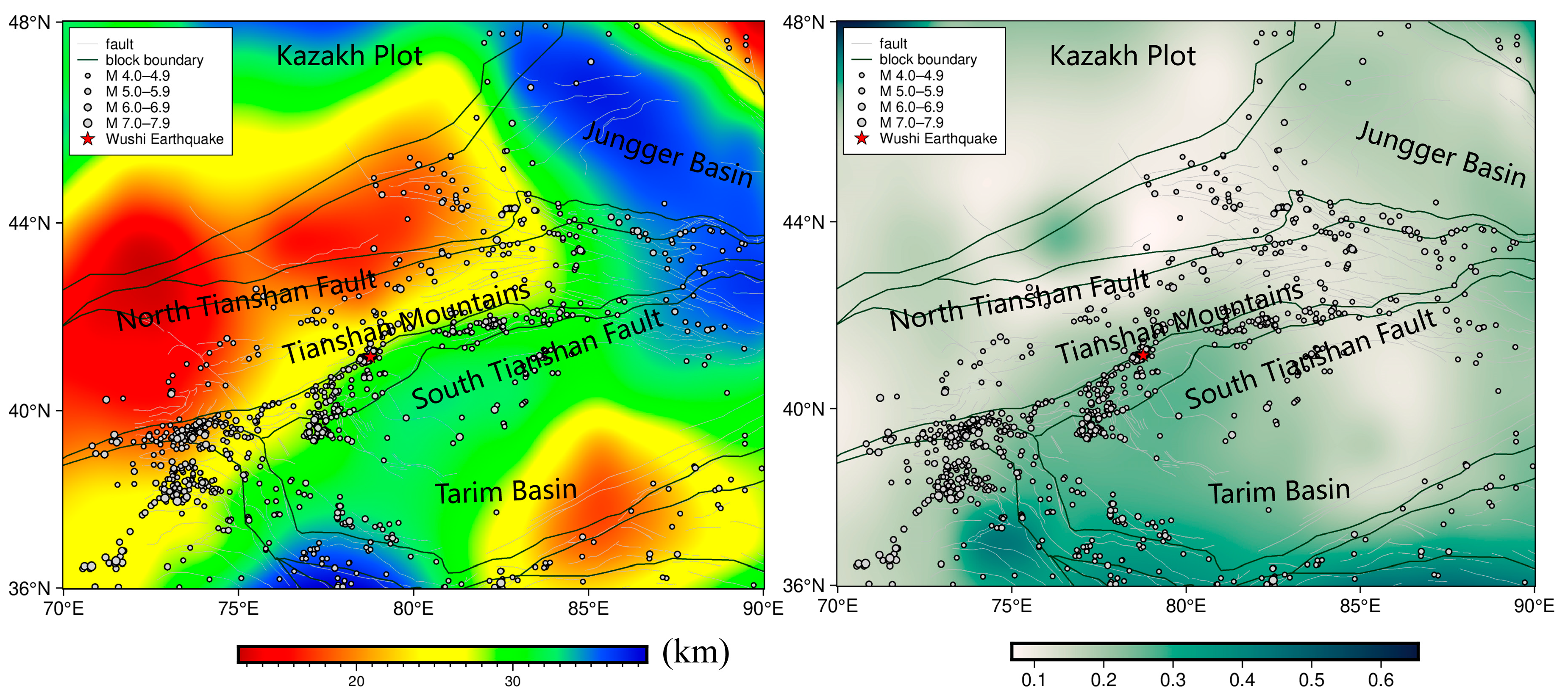
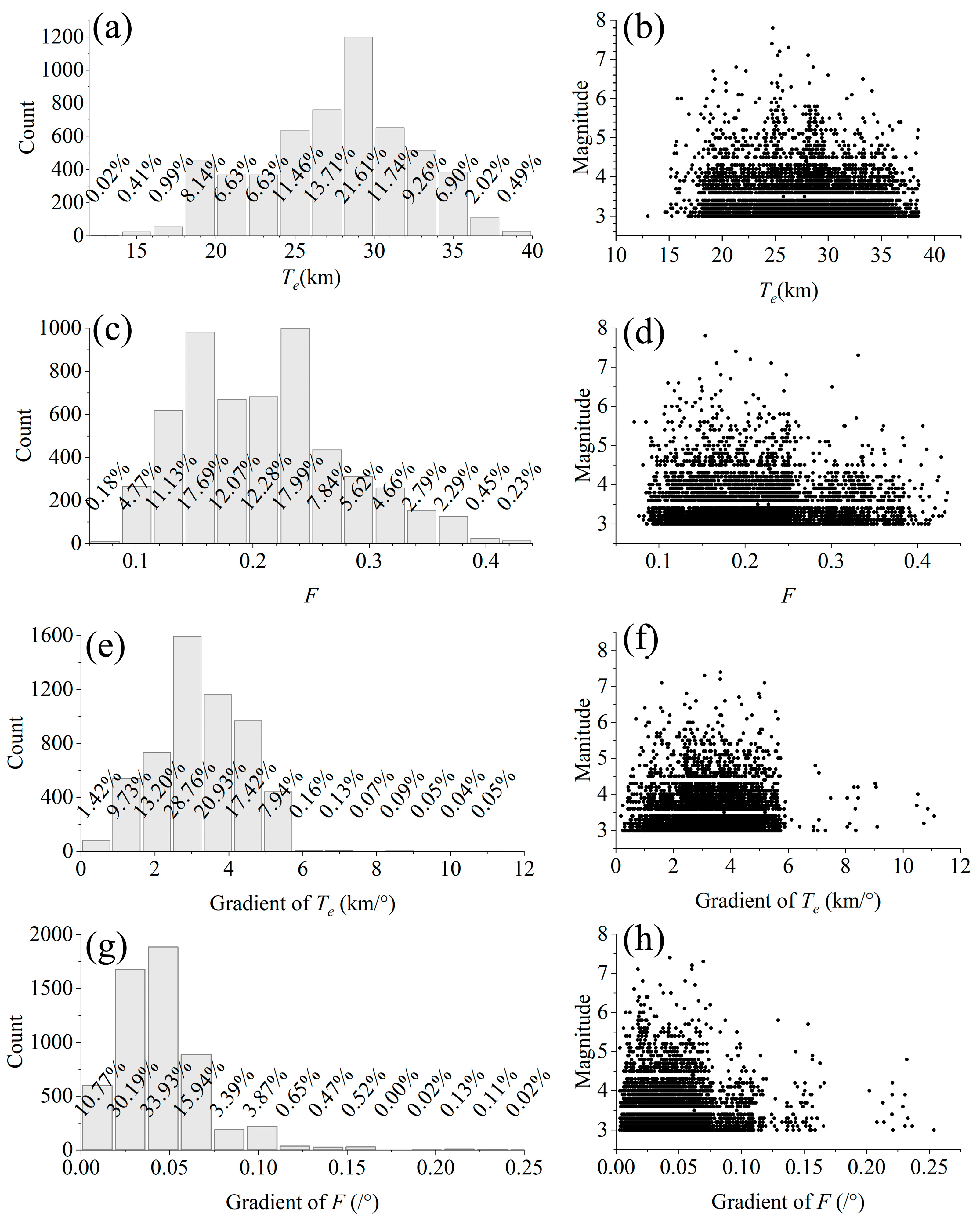
3.3. Analysis of the Relationship with Earthquakes

The effective elastic thickness of the lithosphere reflects the strength differences of the lithosphere, and the region with lower strength is more likely to undergo equilibrium adjustment of the crust; this adjustment process is inevitably accompanied by the accumulation of regional tectonic forces [1,2]. When tectonic forces (e.g., plate movement, magmatic activity, etc.) cause the internal stress of the rock to exceed its strength limit, the rock ruptures or slips along the existing faults, releasing the elastic strain energy, and triggering earthquakes. Thus, earthquakes are essentially a direct manifestation of the sudden release of stresses accumulated in the crust or lithosphere [44,45]. Compared with other landmasses in the world, the seismic activity in Tianshan and neighboring areas is characterized by large magnitudes and short intervals. Therefore, it is of great significance to analyze the relationship between earthquakes and the regional seismogenic environment. Figure 4, Figure 6 and Figure 7 show the relationship between the source locations and magnitudes of seismic activities (with M ≥ 4) occurring in the study area since 2000, as well as Te, F, the Te gradient, and the F gradient, respectively. It can be seen that earthquakes are concentrated in the landmass junction zones, and the number of earthquakes occurring in the interior of the landmass is less, indicating that tectonic forces in the landmass junction zones are much greater than those in the interior of the landmass, and that a large-scale equilibrium process of material flow and exchange must exist in the interior of the lithosphere [46]. Some scholars have analyzed the correlation between the effective elastic thickness of the lithosphere and earthquakes. Yang et al. [47] studied the Bouguer gravity anomaly and Te distribution in the eastern part of the Bayan Kara Massif using the SIO gravity elevation model and found that earthquakes mostly occur in the Longmenshan tectonic zone and at block boundaries with low Te (~20 km), which are associated with high stress release. Su et al. [48] calculated the effective elastic thickness of the northeastern margin of the Tibetan Plateau using the spectral method of the Fan wavelet and analyzed the correspondence between Te values and seismic activities; they concluded that earthquakes generally occur in regions with relatively low Te values.

From Figure 7a, it can be seen that earthquakes are active in regions with smaller Te values, and that more than 90% of earthquakes occur in regions with Te values of 18–36 km. The overall relationship shows an approximate normal distribution, consistent with the results of previous studies [37,49,50]. The low occurrence of earthquakes in regions with Te values of 0–15 km may be due to the fact that the lithosphere is too weak to accumulate the stresses required to trigger an earthquake. Figure 7b shows that earthquake magnitude does not correlate well with Te values. Figure 7c,d show that seismicity in the study area corresponds weakly with the load ratio F. Moreover, the effect of the load ratio F on seismicity is not clear because the overall load ratio F values in the study area are small. Figure 7e–h show that earthquakes in the study area seem to occur more frequently in low-gradient regions, probably due to the small overall Te values in the study area. The transition of lithospheric strength in all directions is gentle; the large Te-gradient region occupies a very small part of the study area, while the small Te-gradient region occupies a large part of the area; thus, most earthquakes occur in small Te-gradient regions, and the relationship between earthquakes and both Te and F gradients needs to be further explored. The F gradient needs to be further explored. In conclusion, earthquakes in the study area occur mostly in regions with relatively low lithospheric Te values and are more likely to occur in block junctions within low-Te zones, showing a weaker relationship with F, the Te gradient, and the F gradient.

4. Gravity Field and Apparent Density Variation Characteristics

The Earth’s gravity field is not constant, but it is affected by the mass distribution, density structure, and regional migration of material within and on the surface of the Earth. Measurable changes occur on scales ranging from hours to years or even longer, and may occur before and after moderately strong seismic activity [7,51]. The gravity data obtained from ground-flow observations of the gravity network can directly reveal the mass migration process from the shallow to deep layers of the Earth, offering the advantages of high sensitivity and high resolution, and serving as an irreplaceable tool for a deeper understanding of the Earth and timely early warning of seismic hazards. Since the 1980s, the Earthquake Agency of the Xinjiang Uyghur Autonomous Region has conducted mobile gravity observations in March and July each year. This paper is based on data from 2017 to 2025. To eliminate the influence of surface and groundwater changes, we selected observation data from March of each year. Meanwhile, to eliminate the differences in air pressure and temperature, we used the measured air pressure and temperature values for correction. After classical adjustment and Bayes adjustment, we obtained the annual gravity variation at the gravity observation points. Then, we used the equivalent source inversion method to invert the apparent density and obtain the apparent density characteristics [52].

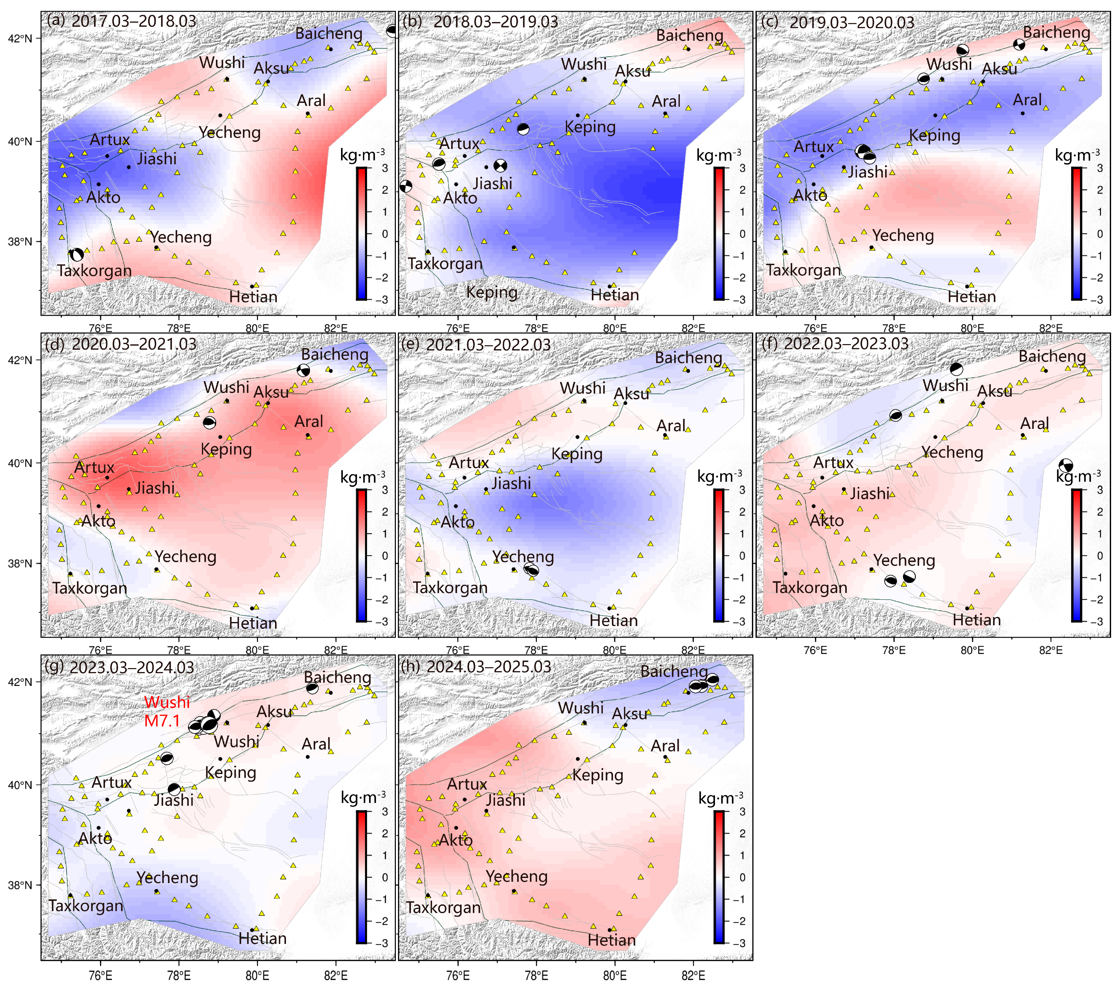
4.1. Analysis of One-Year Scale Gravity Field Variations

Figure 8a shows the image of the gravity field changes in 2017–2018; the positive gravity changes at the measuring points of Kuche–Hetian–Taxkorgan in the hinterland of the Tarim Basin indicate that the crust is subsiding and the density is increasing. Negative changes in gravity along the Kuche–Wushi and Artux–Taxkorgan sections of the northwestern edge of the basin indicate that the crust is in a state of uplift and its density is decreasing. The Wushi–Artux section shows an area of incongruous positive changes; this paper suggests that the Akto Ms6.7 earthquake of November 2016 may have caused the migration of deep crustal material from Akto to Wushi, so that there is a large negative change in gravity in the Akto region as well as a positive change in the Wushi region. Figure 8b shows an image of the gravity field change in 2018–2019; the gravity field of the whole survey area changed in the opposite direction compared with the previous year, indicating that deeper materials of the crust are undergoing a stage of reverse adjustment, and that four moderately strong earthquakes occurred along the western edge of the Tarim Basin, in regions with alternating positive and negative gravity values as well as in regions with large gradients of negative value changes. Figure 8c shows an image of gravity field changes in 2019–2020; the pattern of changes is basically the same as that of the previous year, with only the center of the Tarim Basin region showing positive changes in gravity values. The Artux–Jiashi–Yecheng–Taxkorgan region shows a clear region of alternating positive and negative values, where several moderate-to-strong earthquakes, including the January 2020 Jiashi Ms6.4, have occurred. Figure 8d shows an image of the gravity field changes in 2020–2021. The area of positive gravity value change in the tower further expanded compared with the previous year. Adjustment of the crustal medium occurred in the near-field area of the epicenter of the Jiashi Ms6.4 earthquake, and the gravity values changed positively, likely affected by these two parts of the adjustment. The Aksu area, which is in the northeastern part of the network, shows gravity changes completely opposite to those of the previous year, with an Ms5.4 earthquake occurring in March 2020 and an Ms5.2 earthquake occurring in May of the same year. An Ms5.4 earthquake occurred in March 2020, and an Ms5.2 earthquake occurred in May of the same year. Figure 8e shows that the gravity values began to be adjusted in reverse in 2021–2022, and the gravity changes at most of the sites were opposite to those of the previous year, with two strong and moderate earthquakes of magnitude 5 or higher occurring in the Yecheng region during the adjustment process. Figure 8f shows that the gravity changes in the western part of the network were larger in 2022–2023, while the changes in other regions were less obvious. Moreover, strong and moderate earthquakes occurred in a few areas of gravity reversal and in the transition areas between positive and negative changes.

Figure 8g shows the gravity changes in 2023–2024; the gravity changes in the Baicheng–Aral–Hetian region are basically the same as those of the previous year, but the gravity changes along the Baicheng–Akto–Hetian section of the northwestern edge of the Tarim are opposite to those of the previous year. There are positive and negative transition changes in the Wushi region, and a strong Ms 7.1 earthquake occurred in Hetian in the same year. Figure 8h shows that the changes in gravity at each measurement point during 2023–2024 were again opposite to those of the previous year, and began to be adjusted in the opposite direction, similar to the changes in Figure 8f. This indicates that the deep crustal structure began to recover after the earthquake and was in the stage of accumulating energy, suggesting a greater risk of strong or moderate earthquakes recurring in the vicinity of the measurement area in 2025–2026. In conclusion, medium-to-strong earthquakes are likely to occur in areas of alternating positive and negative gravity changes, during stages of large-scale reverse gravity adjustments, and in the time periods following gravity anomalies.

4.2. Field Source Apparent Density Variation Analysis

The time-varying gravity signals obtained from terrestrial gravity observations provide an important basis for studying the medium changes in seismogenic zones within the Earth’s crust. The apparent density characteristics can be obtained by inverting the time-varying gravity field through the “equivalent source” model. The field source apparent density inversion process involves using spherical-coordinate hexahedral cells to build the field source Green’s function, introducing spatiotemporal smooth a priori conditions to suppress noise interference, and using the Bayesian principle and the asymptotic Bayesian information criterion (ABIC) minimization criterion to optimize the “equivalent source” inversion model calculation.

Since the depth of the Wushi earthquake retrieved in this paper is 11.9 km (Section 5.2), we assume a burial depth of 12 km and a thickness of 1 km for the simulated field source body, which facilitates better analysis of the variation of medium density at the seismic depth. Since 2017, the Wushi region has been in a transition region of positive and negative field source apparent density. The positive and negative boundaries of field source apparent density in 2017–2018 were oriented NW-SE. In 2018–2019, the direction was basically the same as that of the previous year, but the positive and negative areas were reversed; in 2019–2020, the positive and negative boundary areas changed from the NW-SE direction to the E-W direction, with the northern part of the area being the positive area and the southern part of the area being the negative area. In 2020–2021, the boundary direction changed to the NE-SW direction, and the positive and negative areas were again reversed; at this time, the boundary direction was very close to the strike of the Wushi earthquake-generating fault. In 2019–2020, the positive–negative boundary area changed from the NW-SE to E-W strike, with the positive area in the north and the negative area in the south. In 2020–2021, the boundary strike changed to NE-SW, and the positive–negative areas reversed again; at this time, the boundary strike was very close to the strike of the seismogenic fault of Wushi, which is considered a window into the seismogenesis period of Wushi, according to previous studies [53,54,55]. The values of apparent density in 2021–2022 and 2022–2023 were smaller than those in previous years, and the crust may have been in a “solidified” state of high stress–strain [56], with weakened activity but continued increase in internal stresses. On 23 January 2024, an Ms7.1 earthquake occurred in Wushi County; Figure 9h shows that after the earthquake, the apparent density of the region changed dramatically. The positive–negative boundary in the NE-SW direction before the earthquake changed again to the NW-SE direction, with positive apparent density to the south of the boundary and negative density to the north of the boundary, showing a four-quadrant type of change, which proves that the deep structure of the crust had changed after the earthquake.

5. InSAR Coseismic Deformation Monitoring

While gravity field and apparent density changes can only reveal long-term regional evolution (on annual scales), InSAR technology can resolve crustal structural changes that occur instantaneously during earthquakes. After decades of development, InSAR has become a vital tool for obtaining coseismic deformation fields, effectively compensating for the limitations of gravity data, which require long observation cycles and cannot precisely cover the seismic event timeframe.

5.1. Data and Processing Methods

In this paper, we use Sentinel-1 satellite C-band image data (

Table 1. Sentinel-1A data parameters are used in this paper.

Spatial Resolution	Orbit	Master Image	Secondary Image	Time Baseline	Spatial Baseline	Polarization	Beam Mode	Incidence	Azimuth
5 × 20 m	As056	14 January 2024	26 January 2024	12 d	−19.65 m	VV	IW	39.66°	13.57°
	Des136	20 January 2024	25 February 2024	36 d	109.54 m			39.64°	166.40°

), combined with precision orbit data released by the European Space Agency (ESA) to remove the reference ellipsoid phase, the atmospheric delay correction model provided by the Generic Atmospheric Correction Online Service (GACOS) to remove the influence of atmospheric delay on the interferometric images, and the 30 m spatial resolution Shuttle Radar Topography Mission Digital Elevation Model (SRTM DEM) data released by the National Aeronautics and Space Administration (NASA) to remove the influence of terrain effects on the interferograms [57]. The interferometric processing of elevated-orbit SAR images is carried out using GMTSAR (v6.3) software; the Goldstein filtering method [58] is used to remove noise from the interferograms to improve the quality of the interferograms; and the minimum cost flow algorithm [59] is used to perform phase untangling in order to extract the surface deformation information from the interferograms.

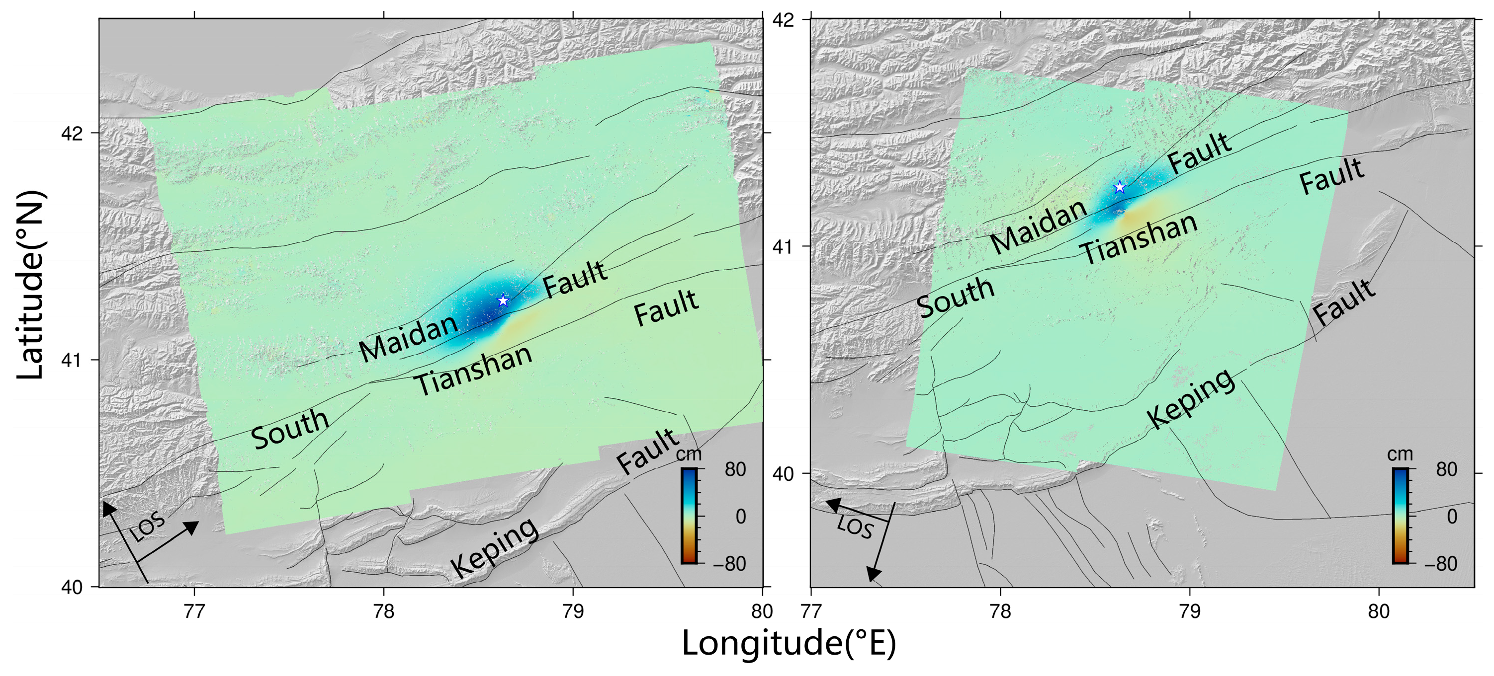
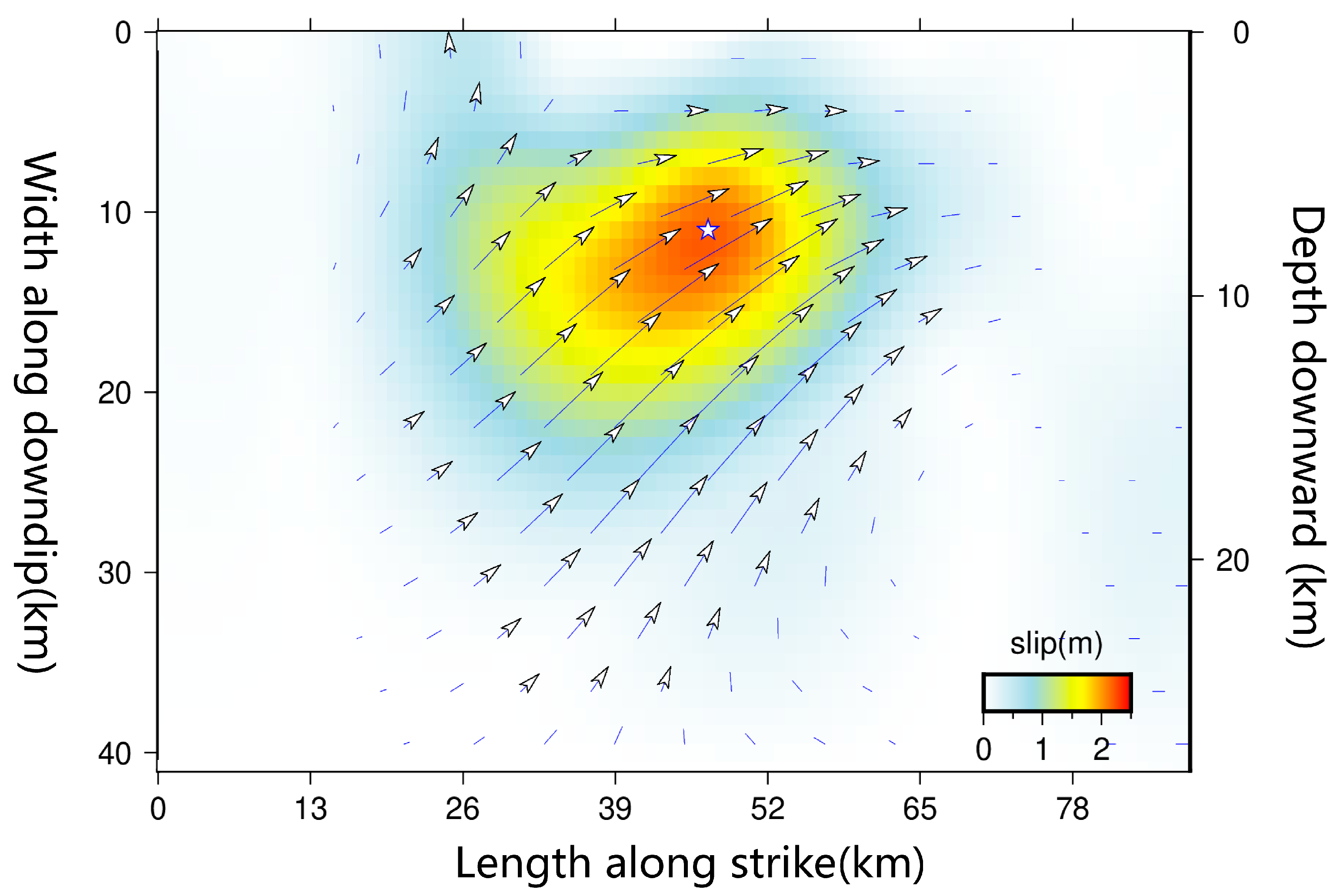
5.2. Coseismic Deformation Field and Fault Slip Modeling

The processed data reveal the coseismic deformation field as shown in Figure 10. The deformation field exhibits good continuity without significant noise points, displaying an overall elliptical pattern striking NE-SW, consistent with the Maidan fault strike. In the ascending track, the maximum line-of-sight (LOS) displacement is 78 cm of uplift and 19 cm of subsidence. In the descending track, the maximum LOS displacement is 62 cm of uplift and 15 cm of subsidence. The uplift significantly exceeds subsidence during this event. Initial inference suggests a thrust-dominated fault motion.

After this, the deformation field is masked using the coherence coefficient to ensure the reliability of the results, and then the deformation field is downsampled using the quadtree downsampling algorithm. The appropriate deformation gradient threshold is set to reduce the observation density while retaining the deformation information in the vicinity of the faults in order to reduce the pressure of the subsequent calculations. The fault plane is discretized into several 1 km × 1 km rectangles, while certain smoothing constraints are imposed on the discretized adjacent rectangles. Some scholars have identified the SW strike node as the seismogenic fault plane through aftershock sequence repositioning [60,61]. Therefore, we assume a fault with a strike range of 180° to 270°, and invert the seismogenic fault using the SDM, based on the characteristics exhibited in the coseismic deformation site. The width of the fault is set to 40 km, the length is set to 85 km, and the search range of the dip angle is between 20° and 70°. The specific values are adjusted according to the fitting degree of the SDM iteration results. The rake angle is not initially set. The location, depth, magnitude, dip angle, and rake angle are output in the SDM iteration. The final optimal solution is obtained as follows: location 78.61°E, 41.22°N, depth 11.9 km; moment magnitude Mw6.99; strike 232°; dip angle 48°; and rake angle 80°. These results are basically the same as the solutions for the seismic mechanism given by various institutions (

Table 2. Explanation of the seismic mechanisms issued by the agencies.

	Location/(°E, °N)	Strike/°	Dip/°	Rake/°	Depth/km	Magnitude/Mw
USGS	78.66, 41.26	235	45	42	13.0	7.0
GFZ	78.73, 41.28	251	38	73	15.0	7.0
GCMT	78.56, 41.19	235	46	44	16.1	7.1
This Paper	78.61, 41.22	232	48	80	11.9	7.0

).

As can be seen from Figure 11, fault slip is mainly concentrated between a 0 and 18 km depth along a fault strike of 25–60 km. The maximum sliding amount is 2.2 m, which is located at a depth of 7 km along the fault strike of 45 km. It is worth noting that slight slips also occur at a 0 km depth between 15 and 30 km and 50 and 55 km along the fault strike, indicating that the earthquake caused surface rupture. From this fault slip model, it can be determined that the earthquake is an anticlinal event with left-rotation slip, and the amount of slip decreases with depth away from the source of the earthquake.

6. Discussion

The results of calculating the effective elastic thickness in this paper show that the Tarim Basin and Junggar Basin regions have higher Te values, while the lower Tianshan Mountains have smaller Te values. These findings are consistent with the results of previous calculations. However, some scholars have reported a better correlation between earthquakes and Te gradients, i.e., the large Te gradient zone corresponds to the seismic intensity zone [6,37]. The results of this paper do not show this regularity (Figure 7e) because they calculated the effective elastic thickness across the Chinese mainland region, where the range of Te values is between 10 and 110 km, encompassing all the lithospheric strengths from soft to extremely hard. The Chinese continent also experiences a large frequency of earthquakes, making it easier to analyze the regularity. In contrast, this study has a smaller scope, a smaller span of Te values (13~39 km), and a limited number of earthquakes that can be analyzed. In addition, different spectral analysis methods may also produce different values. For instance, the multi-window spectral method, although it has high noise resistance, lacks the ability to localize when dealing with complex structural regions. Therefore, there may be some differences when using the multi-window spectral method for calculation.

In this paper, only the one-year scale variation of the gravity field is analyzed, and field source apparent density is inverted using gravity observation data, while some scholars have processed the gravity data with bit-field separation, such as optimized filtering [62] and wavelet multiscale decomposition [63], to obtain the structure at different depths under the lithosphere. Wavelet multiscale decomposition is able to achieve the separation of shallow disturbances from deep tectonic signals by frequency-space dual-domain analysis and decompose the gravity anomalies of the surface sedimentary layer, mid-crust, and mantle to better understand the subsurface structure. Next, we can use wavelet decomposition to obtain the gravity anomalies of each stratum and then use the equivalent source model to invert the apparent density at the corresponding depth to analyze the deep material structure and tectonic information. In addition, field source apparent density is not the real density of the rock layer, but the size of the apparent density reflects the average density difference between the target field source and its surrounding background rocks. The positive and negative values reflect gravity anomalies caused by high-density and low-density bodies. We found that the positive and negative boundaries of field source apparent density before the Wushi earthquake shifted to a direction similar to that of the originating fault, which indicates that earthquakes are also related to differences in the density of materials in the region; this can be investigated in more depth in the future. At present, tectonic activities in the Tianshan Mountains and their adjacent areas remain intense, and many faults are in an active state. For the monitoring of active faults, we can also analyze their gravitational changes on two-year and three-year scales, which can provide a more detailed understanding of their status. In addition, deep and large faults at plate boundaries (such as subduction zones) can cause sudden changes in crustal thickness. When high-density oceanic crusts subduct beneath a continent, significant positive gravity anomalies are formed. In the rift zone, the crust is stretched and thinned, and low-density substances surge up, corresponding to negative anomalies. All these changes can be clearly observed by gravity instruments. Observing gravity values and capturing abnormal signals can provide strong support for the analysis of seismic and geological tectonic activities.

The same color scale as above is used to superimpose the Wushi seismic lift-track coseismic deformation field onto the apparent density (Figure 12). It can be seen that there is a correspondence between the deformation field and the apparent density. The location of the seismicity is exactly on the transition boundary between positive and negative values. Crustal uplift occurs in the negative apparent density area, and subsidence occurs in the positive apparent density area. We believe that earthquakes result from transient adjustments in the deep material structure of the Earth’s crust when accumulated stress exceeds the capacity of rigid blocks. Subsidence occurs as a result of the outflow of material from high-visibility densities, and uplift occurs as a result of the inflow of material from low-visibility densities. However, it is not clear whether this is a general pattern; in-depth studies are needed to analyze the source mechanism solutions of a large number of earthquakes and fault slip models.

7. Conclusions

The 2024 Wushi Ms7.1 earthquake occurred in the southern Tianshan tectonic belt and had a significant impact on the neighboring areas. In this paper, we analyzed the background of earthquake generation in Tianshan and neighboring areas based on the effective elastic thickness of the lithosphere, time-varying gravity, apparent density, and InSAR. We came to the following conclusions:

(1) The effective elastic thickness of the lithosphere in the Tianshan Mountains ranges from 13 to 28 km, indicating relatively weak integrated mechanical strength. The Tarim Basin and Junggar Basin have relatively high mechanical strength due to their Precambrian crystalline rock system as the basement, with Te values greater than 30 km. The corresponding load ratios are all less than 0.5, suggesting that surface loads are dominant. By analyzing the relationship between the number of earthquakes and the Te value, it is found that earthquakes are prone to occur in regions with relatively weak lithospheric strength.

(2) Medium-to-strong earthquakes tend to occur in areas of alternating positive and negative gravity changes and during the phase of large-scale gravity reversal. It is expected that the risk of a moderate-to-strong earthquake occurring again in the vicinity of the survey area between 2025 and 2026 is relatively high. Before the Wushi earthquake, the positive and negative boundaries of field source apparent density shifted to a nearly parallel strike with the seismogenic fault, and then the earthquake was triggered after a “solidification” process. This finding provides a basis for in-depth studies on the relationship between the seismogenic mechanism and field source apparent density, as well as a reference for monitoring key seismogenic regions.

(3) The Wushi earthquake was a thrust event with left-handed strike-slip. Analysis of the coseismic deformation field of the Wushi earthquake reveals that subsidence occurs entirely within the positive apparent density zone, and vice versa for uplift. Whether this is a universal law is not clear. It is necessary to analyze the source mechanism solutions and fault slip models of a large number of earthquakes. This also provides a direction for future research.

References

1. Lowry, A.R.; Smith, R.B. Strength and rheology of the western US Cordillera. J. Geophys. Res. Solid Earth 1995, 100, 17947–17963. [Google Scholar] [CrossRef]
2. Cloetingh, S.; Ziegler, P.A.; Beekman, F.; Andriessen, P.A.M.; Matenco, L.; Dèzes, P.; Sokoutis, D. Lithospheric memory, state of stress and rheology: Neotectonic controls on Europe’s intraplate continental topography. Quat. Sci. Rev. 2005, 24, 241–304. [Google Scholar] [CrossRef]
3. Handy, M.R.; Brun, J.P. Seismicity, structure and strength of the continental lithosphere. Earth Planet. Sci. Lett. 2004, 223, 427–441. [Google Scholar] [CrossRef]
4. Maggi, A.; Jackson, J.A.; Mckenzie, D.; Priestley, K. Earthquake focal depths, effective elastic thickness, and the strength of the continental lithosphere. Geology 2000, 28, 495–498. [Google Scholar] [CrossRef]
5. McKenzie, D.; Fairhead, D. Estimates of the effective elastic thickness of the continental lithosphere from Bouguer and free air gravity anomalies. J. Geophys. Res. Solid Earth 1997, 102, 27523–27552. [Google Scholar] [CrossRef]
6. Chen, B.; Che, C.; Kaban, M.K.; Du, J.; Liang, Q.; Thomas, M. Variations of the effective elastic thickness over China and surroundings and their relation to the lithosphere dynamics. Earth Planet. Sci. Lett. 2013, 363, 61–72. [Google Scholar] [CrossRef]
7. Barnes, D.F. Gravity changes during the Alaska earthquake. J. Geophys. Res. 1966, 71, 451–456. [Google Scholar] [CrossRef]
8. Chen, Y.T.; Gu, H.D.; Lu, Z.X. Variations of gravity before and after the Haicheng earthquake, 1975, and the Tangshan earthquake, 1976. Phys. Earth Planet. Inter. 1979, 18, 330–338. [Google Scholar] [CrossRef]
9. Heki, K.; Matsuo, K. Coseismic gravity changes of the 2010 earthquake in central Chile from satellite gravimetry. Geophys. Res. Lett. 2010, 37, 24. [Google Scholar] [CrossRef]
10. Zhao, J.; Liu, G.; Lu, Z.; Zhang, X.; Zhao, G. Lithospheric structure and dynamic processes of the Tianshan orogenic belt and the Junggar basin. Tectonophysics 2003, 376, 199–239. [Google Scholar] [CrossRef]
11. Wang, B.; Song, F.; Ni, X. Paleozoic accretionary orogenesis and major transitional tectonicevents of the Tianshan orogcn. Acta Geol. Sin. 2022, 96, 3514–3540. [Google Scholar]
12. Wang, Z.; Li, C.; Pak, N.; Ivleva, E.; Yu, X.; Zhou, G.; Xiao, W.; Han, S.; Halilov, Z.; Takenov, N.; et al. Tectonic division and Paleozoic ocean- continent transition in Western Tianshan Orogen. Geol. China 2017, 4, 623–641, (In Chinese with English Abstract). [Google Scholar]
13. Zhang, C.; Zou, H.; Li, H. Tectonic framework and evolution of the Tarim Block in NW China. Gondwana Res. 2013, 23, 1306–1315. [Google Scholar] [CrossRef]
14. Graham, S.A.; Hendrix, M.S.; Wang, L. Collisional successor basins of western China: Impact of tectonic inheritance on sand composition. Geol. Soc. Am. Bull. 1993, 105, 323–344. [Google Scholar] [CrossRef]
15. Yin, A.; Nie, S.; Craig, P. Late Cenozoic tectonic evolution of the southern Chinese Tian Shan. Tectonics 1998, 17, 1–27. [Google Scholar] [CrossRef]
16. Lei, J.; Zhao, D. Teleseismic P-wave tomography and the upper mantle structure of the central Tien Shan orogenic belt. Phys. Earth Planet. Inter. 2007, 162, 165–185. [Google Scholar] [CrossRef]
17. Hapaer, T.; Tang, Q.; Sun, W. Opposite facing dipping structure in the uppermost mantle beneath the central Tien Shan from Pn traveltime tomography. Int. J. Earth Sci. 2022, 111, 2571–2584. [Google Scholar] [CrossRef]
18. Laske, G.; Masters, G.; Ma, Z. Update on CRUST1. 0—A 1-degree global model of Earth’s crust. Geophys. Res. Abstr. 2013, 15, 2658. [Google Scholar]
19. Wang, L.; Chen, S.; Zhang, B. Analysis of the Variation of Gravity Field Source Before the 2013 Lushan Ms 7.0 Earthquake. Earthquake 2021, 41, 78–92. [Google Scholar]
20. Wang, R.; Diao, F.; Hoechner, A. SDM-A geodetic inversion code incorporating with layered crust structure and curved fault geometry. In Proceedings of the EGU General Assembly, Vienna, Austria, 7 April 2013. Conference Abstracts EGU2013-2411. [Google Scholar]
21. Liu, D.; Zhao, L.; Yuan, H. Receiver function mapping of the mantle transition zone beneath the Tian Shan orogenic belt. J. Geophys. Res. Solid Earth 2022, 127, e2022JB024635. [Google Scholar] [CrossRef]
22. Xie, W.; Zhu, J.; Luo, Z.; Xu, Y. Petrogenesis and geological implications of the Late Carboniferous Baiyanggouvolcanic rocks. Acta Petrol. Sin. 2018, 34, 126–142. [Google Scholar]
23. Xu, Y.; Rocker, S.W.; Wei, R.-P.; Zhang, W.-L.; Wei, B. Analysis of seismic activity in the crust from earthquake relocation in the Central Tian Shan. Chin. J. Geophys 2005, 48, 1308–1315. [Google Scholar] [CrossRef]
24. Lin, W.; Li, L.; Zhang, Z.; Shi, Y.; Li, Q.; Xue, Z.; Wang, F.; Wu, L. Paleozoic tectonic of evolution of Tianshanorogen: In the view from a structure analysis of the HP-UHP metamorphic belt of SW Chinese Tianshan. Acta Petrol. 2015, 31, 2115–2128. [Google Scholar]
25. Lv, H.; Li, Y. Deformation characteristics of the active backslope belt in the northern foothills of the Tianshan Mountains. Quat. Sci. 2010, 30, 1003–1011. [Google Scholar]
26. Wu, C. Characteristics of Late Quaternary activity and role in the tectonic deformation of the NED-trending faults in the southwestern Tien Shan. Prog. Earthq. Sci. 2017, 09, 46–48. [Google Scholar]
27. Pan, Y. Bayesian Estimation of the Effective Elastic Thickness of the Lithosphere and Application to Typical Continental Regions. Ph.D. Thesis, Institute of Geophysics, China Earthquake Administration (CEA), Beijing, China, June 2024. [Google Scholar]
28. Dorman, L.M.; Lewis, B.T. Experimental isostasy: 1. Theory of the determination of the Earth’s isostatic response to a concentrated load. J. Geophys. Res. 1970, 75, 3357–3365. [Google Scholar] [CrossRef]
29. McKenzie, D.; Bowin, C. The relationship between bathymetry and gravity in the Atlantic Ocean. J. Geophys. Res. 1976, 81, 1903–1915. [Google Scholar] [CrossRef]
30. Parker, R.L. The rapid calculation of potential anomalies. Geophys. J. Int. 1973, 31, 447–455. [Google Scholar] [CrossRef]
31. Kirby, J.F.; Swain, C.J. A reassessment of spectral Te estimation in continental interiors: The case of North America. J. Geophys. Res. Solid Earth 2009, 114, B08401. [Google Scholar] [CrossRef]
32. Bonvalot, S.; Balmino, G.; Briais, A. World Gravity Map: Commission for the Geological Map of the World; 25 April 2012; BGI–CGMW-CNES-IRD: Paris, France, 2012. [Google Scholar]
33. Wang, Z. Theory and Methods for Determining the Earth’s Gravity Field from Satellite Tracking Satellite Measurements. Ph.D. Thesis, Wuhan University, Wuhan, China, December 2005. [Google Scholar]
34. Luo, F.; Yn, J.; Zhang, C. The Effective Elastic Thickness of Lithosphere and Its Tectonic Implications in the South China Block. Acta Geosci. Sin. 2022, 43, 771–784. [Google Scholar]
35. Kirby, J.F.; Swain, C.J. Improving the spatial resolution of effective elastic thickness estimation with the fan wavelet transform. Comput. Geosci. 2011, 37, 1345–1354. [Google Scholar] [CrossRef]
36. Chen, B.; Liu, J.; Chen, C. Elastic thickness of the Himalayan–Tibetan orogen estimated from the fan wavelet coherence method, and its implications for lithospheric structure. Earth Planet. Sci. Lett. 2015, 409, 1–14. [Google Scholar] [CrossRef]
37. Shi, W.; Chen, S.; Han, J. Effective elastic thickness of lithosphere and mechanical characteristics of strong seismic tectonic zones in mainland China. Earthquake 2021, 41, 1–12. [Google Scholar]
38. Liu, D. Studies on the Lithospheric Structure and Seismodynamic Environment of Tianshan and Neighboring Areas. Ph.D. Thesis, University of Science and Technology of China (USTC), Hefei, China, September 2024. [Google Scholar]
39. Zuo, Y.; Li, J.; Li, W. Mesozoic and Cenozoic ”thermal” Lithospheric thickness evolution in the Tarim basin. Prog. Geophys. 2015, 30, 1608–1615. [Google Scholar]
40. Zhao, J.; Huang, Y.; Ma, Z. Discussion on the basement structure and property of northern Junggar basin. Chin. J. Geop. Hys. 2008, 51, 767–1775. [Google Scholar]
41. Yang, H.; Teng, J.; Wang, Q. Numerical simulation study of sufficient and necessary conditions for material flow in the lower crust of the Tibetan Plateau. In Proceedings of the 27th Annual Meeting of the Chinese Geophysical Society, Chengdu, China, 17 October 2012. [Google Scholar]
42. Jin, J.; Liu, M.; Liu, Y. Present-day temperature-pressure field and its controlling factors of the lower composite reservoir in the southern margin of Junggar Basin. Chin. J. Geol. 2021, 56, 28–43. [Google Scholar]
43. Wang, L.; Li, C.; Shi, Y. Characterization of geodetic heat flow density distribution in the Tarim Basin. ACTA Geophys. A Sin. 1995, 06, 855–856. [Google Scholar]
44. Han, K.; Liu, D.; Ailixiati, Y. InSAR Coseismic Deformation and Slip Distribution Characteristics of the Jishishan MS6.2 Earthquake in 2023. J. Geod. Geodyn. 2025. [Google Scholar] [CrossRef]
45. Zhang, P.; Deng, Q.; Zhang, Z. Active faults, earthquake hazards and associated geodynamic processes in continental China. Sci. Sin. Terrae 2013, 43, 1607–1620. (In Chinese) [Google Scholar]
46. Zhang, Y.; Wang, Q.; Teng, J. Crustal equilibrium anomalies and their relation to earthquake distribution in the eastern part of Sichuan and Tibet. Chin. J. Geophys. 2010, 53, 2631–2638. [Google Scholar]
47. Yang, G.; Sheng, C.; Li, Z. Gravity equilibrium and effective elastic thickness of the lithosphere in the eastern part of the Ba Yan Ka La Massif and neighboring areas. Chin. J. Geophys. 2020, 63, 956–968. [Google Scholar]
48. Su, Z.; Lu, B.; Li, B. Effective elastic thickness of the lithosphere along the northeastern margin of the Tibetan Plateau in relation to seismic distribution. Chin. J. Geophys. 2024, 67, 520–533. [Google Scholar]
49. Xu, S. Spectral Correlation Method to Calculate the Effective Elastic Thickness of South China Sea. Ph.D. Thesis, China University of Geosciences, Beijing, China, May 2019. [Google Scholar]
50. Hu, M.; Jin, T.; Hao, H. Effective elastic thickness of the lithosphere at the southeastern margin of the Tibetan Plateau and its tectonic significance. Chin. J. Geophys. 2020, 63, 969–987. [Google Scholar]
51. Zhu, Y.; Zhang, Y.; Yang, X.; Liu, F.; Zhang, G.; Zhao, Y.; Wei, S.; Mao, J.; Zhang, S. Progress of time-varying gravity in seismic research. Rev. Geophys. Planet. Phys. 2022, 53, 278–291. [Google Scholar]
52. Liu, D.; Chen, S.; Wang, X. The apparent density variation of the focal area before and after Jiashi MS 6.4 earthquake and its tectonic significance. Seismol. Geol. 2021, 43, 311–328. [Google Scholar]
53. Xu, S.; Huang, J.; Zheng, Q. Reconstruction of strong pre-seismic gravity change data and inversion of apparent density–An example of the 2021 Yangbi 6.4 magnitude earthquake. J. Seismol. Res. 2025, 48, 631–640. [Google Scholar]
54. Zhu, Y.; Shen, C.; Zhang, G. Rethinking the development of mobile gravity monitoring and forecasting in China. J. Geod. Geodyn. 2018, 38, 441–446. [Google Scholar]
55. Hu, M.; Hao, H.; Li, H. Analysis of Gravity Change Anomaly Indicators for Seismic Analysis and Forecasting. Earthq. Res. China 2019, 35, 417–430. [Google Scholar]
56. Hu, M.; Hao, H.; Han, Y. Gravity flexura lisostasy background of the 2021 Madoi (Qinghai) Ms 7.4 earthquake and gravity change before the earthquake. Chin. J. Geophys. 2021, 64, 3135–3149. [Google Scholar]
57. Farr, T.G.; Rosen, P.A.; Caro, E. The shuttle radar topography mission. Rev. Geophys. 2007, 45, RG2004. [Google Scholar] [CrossRef]
58. Goldstein, R.M.; Werner, C.L. Radar interferogram filtering for geophysical applications. Geophys. Res. Lett. 1998, 25, 4035–4038. [Google Scholar] [CrossRef]
59. Costantini, M.A. novel phase unwrap method based on network programming. IEEE Trans. Geosci. Remote Sens. 1998, 36, 813–821. [Google Scholar] [CrossRef]
60. Xue, Z.; Chuan, W.; Jian, M. Earthquake sequence relocation and seismogenic structure of the 2024 Ms7.1 Wushi earthquake on January 23, 2024, Xinjiang. Seismol. Geol. 2025, 47, 488–506. [Google Scholar]
61. Jiu, Y.; Yang, W.; Cai, X. Coseismic deformation and slip distribution of the January 2024 Xinjiang WushiMS7.1 earthquake revealed by InSAR observations. Chin. J. Geophys. 2025, 68, 2532–2543. [Google Scholar]
62. Meng, X.; Guo, L.; Chen, Z. A method for gravity anomaly separation based on preferential continuation and its application. Appl. Geophys. 2009, 6, 217–225. [Google Scholar] [CrossRef]
63. Kong, X.; Liu, D.; Ailixiati, Y. Study on the characteristics of gravity field and apparent density in Urumqi and its surrounding areas. Seismol. Geol. 2024, 46, 1123–1150. [Google Scholar]
Figure 1. Regional topography.
Remotesensing 17 02655 g001
Figure 2. (a) Flexural response of surface loads; (b) flexural response of subsurface loads. Quote from [27].
Remotesensing 17 02655 g002
Figure 3. (ac): Te, F, χ 2 for k 0 = 2.668; (df): Te, F, χ 2 for k 0 = 3.081; (gi): Te, F, χ 2 for k 0 = 3.773; (jl): Te, F, χ 2 for k 0 = 5.336; (mo): Te, F, χ 2 for k 0 = 7.547.
Remotesensing 17 02655 g003
Figure 4. Te (left) and F (right) in Tianshan and neighboring areas.
Remotesensing 17 02655 g004
Figure 5. Curve fitting of admittance and coherence in different plots (a) Kazakh Plot; (b) Junggar Basin; (c) Tianshan Mountains; (d) Tarim Basin (measured values in blue; predicted values in orange).
Remotesensing 17 02655 g005
Figure 6. Te gradient (left) and F gradient (right) in Tianshan and neighboring areas.
Remotesensing 17 02655 g006
Figure 7. (a) Proportion of earthquake occurrences in different Te sections; (b) distribution of magnitudes in different Te sections; (c) proportion of earthquake occurrences in different F sections; (d) distribution of magnitudes in different F sections; (e) proportion of earthquake occurrences in different Te gradient sections; (f) distribution of magnitudes in different Te gradient sections; (g) proportion of earthquake occurrences in different F-gradient sections; (h) distribution of magnitudes in different F-gradient sections.
Remotesensing 17 02655 g007
Figure 8. Gravity field changes in 2017–2025 (the black and white beach balls represent the focal mechanism solutions, and the light yellow circles indicate other earthquakes of magnitude 5 or greater that occurred during that time period).
Remotesensing 17 02655 g008
Figure 9. Field source apparent density in 2017–2025 (the black and white beach balls represent the earthquake source mechanism solutions for earthquakes of magnitude 5 and above, and the yellow triangles represent the gravity measurement points).
Remotesensing 17 02655 g009
Figure 10. Coseismic deformation field of the ascending (left) and descending (right) rails of the Wushi earthquake (the white star represents the location of the epicenter).
Remotesensing 17 02655 g010
Figure 11. Slip modeling of coseismic faults for the Wushi earthquake (the white star represents the location of the epicenter).
Remotesensing 17 02655 g011
Figure 12. Ascending (a), descending (b) track deformation field and apparent density superposition results.
Remotesensing 17 02655 g012