A Hybrid Spatio-Temporal Graph Attention (ST D-GAT Framework) for Imputing Missing SBAS-InSAR Deformation Values to Strengthen Landslide Monitoring

Abstract

Reservoir-induced landslides threaten infrastructures and downstream communities, making continuous deformation monitoring vital. Time-series InSAR, notably the SBAS algorithm, provides high-precision surface-displacement mapping but suffers from voids due to layover/shadow effects and temporal decorrelation. Existing deep-learning approaches often operate on fixed-size patches or ignore irregular spatio-temporal dependencies, limiting their ability to recover missing pixels. With this objective, a hybrid spatio-temporal Graph Attention (ST-GAT) framework was developed and trained on SBAS-InSAR values using 24 influential features. A unified spatio-temporal graph is constructed, where each node represents a pixel at a specific acquisition time. The nodes are connected via inverse distance spatial edges to their K-nearest neighbors, and they have bidirectional temporal edges to themselves in adjacent acquisitions. The two spatial GAT layers capture terrain-driven influences, while the two temporal GAT layers model annual deformation trends. A compact MLP with per-map bias converts the fused node embeddings into normalized LOS estimates. The SBAS-InSAR results reveal LOS deformation, with 48% of missing pixels and 20% located near the Dasu dam. ST D-GAT reconstructed fully continuous spatio-temporal displacement fields, filling voids at critical sites. The model was validated and achieved an overall R² (0.907), ρ (0.947), per-map R² ≥ 0.807 with RMSE ≤ 9.99, and a ROC-AUC of 0.91. It also outperformed the six compared baseline models (IDW, KNN, RF, XGBoost, MLP, simple-NN) in both RMSE and R². By combining observed LOS values with 24 covariates in the proposed model, it delivers physically consistent gap-filling and enables continuous, high-resolution landslide monitoring in radar-challenged mountainous terrain.

1. Introduction

Landslides are gravity-driven movements of rock, soil, debris or a mixture of these materials along the slopes. According to the widely used Varnes [1] classification [2,3], they can be grouped into falls (free-fall of material), topples (rotation about a pivot), slides (rotational and translational), spreads (lateral extension), and flows (deformation of saturated material). Mechanically, failure occurs when driving shear stresses exceed the shear strength of the slope material. Reservoir-induced landslides pose a significant threat to dam infrastructure and downstream communities. Gradual slope movements during construction or pre-impoundment stages can serve as early warning of future instability [4,5]. For example, multi-temporal Interferometric Synthetic Aperture Radar (InSAR) studies detected slow creep before impoundment at Xiluodu and Baihetan (China) reservoirs [6,7], and an average of five major geohazards per year occurred along the Three Gorges before 2003 filling [8]. Sentinel-1 InSAR further refined landslide inventories at Lianghekou before and after reservoir filling [9], underscoring the significance of InSAR in hazard assessment [10]. Therefore, as the Dasu reservoir on the Indus River nears completion, implementation of high-resolution deformation monitoring is essential to identify vulnerable slopes, guide final design refinements, and implement mitigation measures before water-level changes impose additional loads on slopes.

Time-series InSAR, especially the Small-Baseline Subset (SBAS) algorithm, has become the standard approach for mapping high-precision surface-deformation over long periods when a sufficient number of high-coherence interferograms is available [11,12]. However, when only short stacks or low-coherence pairs are available, the achievable precision is notably lower, and the noise level can increase accordingly. SBAS constructs interferogram networks with small baselines and short revisit times to suppress atmospheric noise and generate line-of-sight (LOS) displacement time series, which are utilized to detect pre-failure ground motion [13,14,15,16]. Nevertheless, steep reservoir banks, dense vegetation, and rapid water-level drawdown induce layover, shadowing, and temporal decorrelation, resulting in spatial–temporal voids in SBAS products and disrupting continuous monitoring [17,18,19]. To bridge these gaps, a variety of gap-filling techniques have been employed. Classical geostatistical methods, such as inverse-distance weighting, ordinary Kriging with spherical variograms, and Gaussian-process regression, provide unbiased, minimum-variance estimates under stationarity assumptions [20,21]. However, these methods handle each acquisition separately, overlook the temporal continuity of deformation, and have computational costs with regional-level datasets.

Recent deep learning methods directly impute missing SBAS-InSAR values. Early CNNs, such as DeepInSAR [22] and GenInSAR [23], improved phase filtering and coherence without clean references, and autoencoders further enhanced raw interferograms. Self-supervised NBDNet [24] delivers real-time inference, while GANs generate realistic InSAR patches [25]. Recurrent models, including those using LSTM/ARIMA and RNN, capture temporal deformation trends [20,26]. Similarly, SVM was integrated with MT-InSAR for susceptibility mapping [27], interpreted reservoir-slope mechanics [28,29], and modeled 3D displacements under topographic constraints [30]. Reviews by Aswathi and Kumar [31], and Miller and Pelletier [32] summarize the advances and highlight the current challenges in InSAR, as well as the application of deep learning models for monitoring hydropower projects. These studies have significantly advanced deep learning for InSAR by improving phase denoising, coherence estimation, temporal modeling, and hazard mapping. Despite these advances, current deep-learning imputation methods for InSAR have some limitations. First, they treat gap detection and imputation as separate steps, relying on fixed-size patches or sequences that misalign with irregular SBAS grids. Second, they integrate spatial and temporal information in a single pass without correcting for acquisition-specific biases. Third, they demand excessive memory and computation for reservoir-scale datasets. To address these challenges, this study introduces ST D-GAT, a hybrid spatio-temporal graph-attention model trained on observed InSAR values with 24 spatio-temporal features, using dual attention streams, per-acquisition bias embeddings, and mini-batch neighbor sampling to handle reservoir-scale datasets efficiently.

The proposed Spatio-Temporal GAT-based InSAR Imputation Model is a unified graph neural framework designed to reconstruct missing InSAR deformation values by modeling complex spatio-temporal dependencies. The model constructs a dynamic graph where each node represents a pixel at a specific time, with edges encoding spatial proximity (via KNN in feature space) and temporal continuity (across years). The input node features are derived from topographic, geological, hydrological, climatic, anthropogenic, hazards, vegetation, and soil covariates, along with spatial embeddings and cyclic temporal encodings. A dual-stream Hybrid Encoder separately processes spatial and temporal neighborhoods using multi-layer GATConv blocks with residual connections and layer normalization. The outputs of both streams are fused and passed through a fully connected Spatial Head (MLP). At the same time, a Learnable Bias Head adjusts for acquisition-specific effects (e.g., seasonal or atmospheric distortions). The model is trained using a Smooth L1 loss on known InSAR pixels only, with imputation performed for missing values. This architecture effectively captures nonlinear geospatial–temporal patterns, yielding robust and physically consistent deformation maps. The study aims to (1) analyze SBAS-InSAR LOS displacement along with static spatial and dynamic temporal features to train a model that directly imputes missing pixels caused by layover, shadow, or decorrelation; (2) design a dual Graph Attention network (GAT) that jointly captures spatial neighbor dependencies within each acquisition and temporal dynamics across successive acquisitions; and (3) demonstrate that the resulting gap-filled InSAR maps preserve physical deformation patterns in previously voided zones.

2. Study Area and Datasets

2.1. Study Area

The study area covers about 1400 km² along the Indus River (Kohistan), northern Pakistan (Figure 1). Geologically, it lies between two major faults: the Main Karakoram Thrust (MKT) to the northwest and the Main Mantle Thrust (MMT) to the southeast [33,34]. Between these faults, the bedrock consists of layers of sedimentary rock, large intrusions of granite and gabbro-norite, and zones of metamorphic and volcanic rocks. Most road-cut slopes are made up of medium to coarse-grained granulites and amphibolite-altered gabbro-norite. Near the surface, these rocks are weathered but, deeper down, they remain fresh yet heavily fractured [35]. Elevations in the study area range from 736 m along the river to 4781 m on nearby peaks, making many slopes steeper than 35°. A historical landslide inventory documents 31 past events, mostly along the left bank of the Indus River upstream of the dam site. Major failures include the toe collapse of the Kaigha landslide, slope failure at the Uchar debris flow, and landsliding near Gayal Sery Village (Figure 1). Morphologically, the river forms a narrow V-shaped gorge upstream of the dam site [36]. Downstream, the valley widens into a broader U-shaped basin before narrowing again near the planned Dasu dam. Vegetation is sparse, and the steep terrain promotes rapid snowmelt in summer. This sudden runoff often triggers landslides and debris flows. Steep slopes cause layover and shadow. Similarly, rapid failures (e.g., debris flows) and slower slope movements alter the surface scattering properties, reducing phase coherence between SAR acquisitions and producing voids in the SBAS time series [37,38]. The proposed ST D-GAT imputation framework leverages 24 influential spatio-temporal features, together with information from neighboring locations and adjacent acquisition dates, to reconstruct the missing pixels.

2.2. SAR Acquisitions

A total of 92 ascending Sentinel-1 C-band SLC images (VV polarization) were collected on track 100, frame 112, from 3 January 2022 to 30 December 2024. All scenes were acquired in Interferometric Wide-Swath (IW) mode with a fixed incidence angle of 37.8° at the scene center and a 12-day revisit cycle. Additionally, each SLC was co-registered with the 30 m Shuttle Radar Topography Mission (SRTM) Digital Elevation Model (DEM) to assist in InSAR processing. The 30 m SRTM DEM was chosen for its global coverage, free availability, and proven accuracy in SBAS-InSAR workflows [39,40].

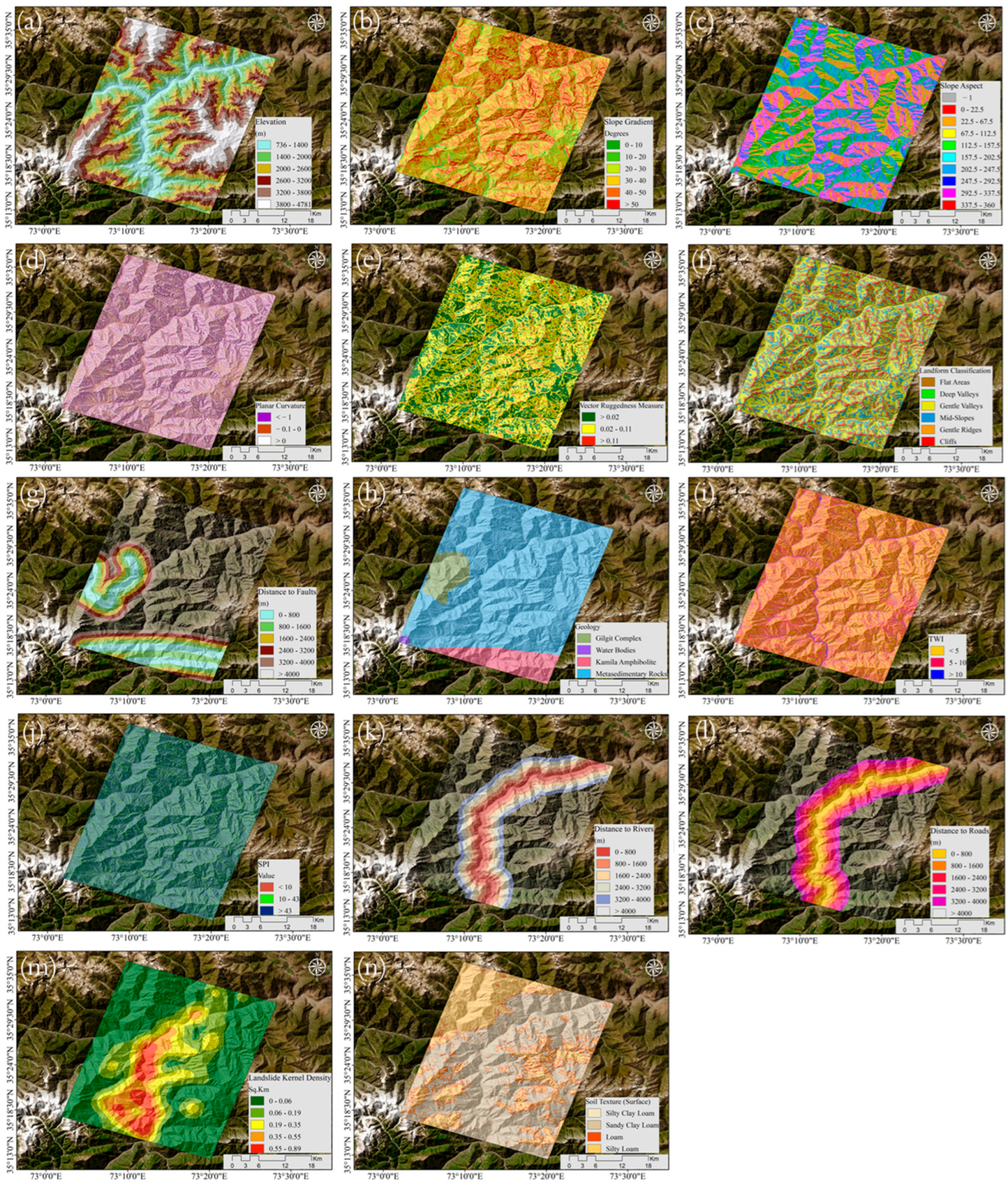
2.3. Static and Dynamic Covariates for InSAR Deformation

Based on the key physical controls that govern interferometric coherence and landslide deformation, a total of 24 InSAR-influential features were selected and grouped into (i) static spatial (14) and (ii) dynamic temporal (10) layers (Figure 2 and Figure 3). All static maps (elevation profile, slope gradient, slope aspect, planar curvature, vector ruggedness measure, landform classification, distance to faults, geology, topographic wetness index, stream power index, distance to rivers, distance to roads, landslide kernel density, and soil texture (surface)) were prepared. These features were resampled to a 30 m grid and clipped to the InSAR boundary, capturing long-term terrain, geological, geomorphological, hydrological, and land cover controls.

Dynamic layers (Modified Normalized Difference Water Index (MNDWI), Annual Rainfall, Evapotranspiration (ET), Temperature (T), Land Use/Land Cover (LULC), Normalized Difference Barren Index (NDBI), Normalized Difference Vegetation Index (NDVI), Profile Soil Moisture (SM_p), Root Zone Soil Moisture (RZSM), and Surface Soil Wetness (SSW) (surface-5 cm below) from 2022–2024) were derived in Google Earth Engine from Landsat 8/9, MODIS, GLDAS, and NASA POWER datasets. For all images, we applied the QA_PIXEL band mask to remove cloudy, shadowed, and snow-covered pixels. We then used a small-window median filter to reduce residual weather noise. Remaining gaps were filled via a five-day locally weighted regression, after which each raster was bias-corrected, bilinearly resampled to 30 m, and stacked cell by cell to form the ten annual dynamic temporal layers. Table S1 in the Supplementary Materials provides detailed information for all 24 covariates. The 14 static spatial with 10 dynamic temporal layers for the spatial map are visualized in Figure 2 and Figure 3, while the 10 dynamic temporal layers for each year (2022, 2023, and 2024) are shown in Supplementary Figures S1–S3.

3. Methodological Framework

Sentinel-1 SAR data (January 2022–December 2024) were processed, and each pixel acquisition was represented by 14 static spatial and 10 dynamic temporal features. SBAS-InSAR deformation imputation is formalized by converting each pixel-acquisition pair into a detailed feature vector and processing the combined data through a unified spatio-temporal graph attention network (GAT) framework. Initially, one spatial baseline and three temporal acquisitions are combined into a single dataset where each row corresponds to a specific pixel at a given acquisition time. Continuous variables are standardized and enriched with coordinate interactions, while skewed measurements receive logarithmic transforms. One-hot region embeddings are generated via K-means clustering on normalized coordinates, and the acquisition index is encoded cyclically, allowing the model to recognize temporal order. All raw and engineered features are concatenated and re-standardized to form each node’s input vector. A graph is then constructed, where every node represents a pixel at a particular time. Spatial edges connect each node to its eight nearest neighbors using inverse-distance weights, and bidirectional temporal edges link the same pixel across consecutive acquisitions. All node features, a mask indicating which InSAR values are observed, and the edge definitions are stored in a single graph data structure. The spatio-temporal GAT Imputer model appends a learnable 16-dimensional time embedding to each node feature, applies two Spatial GAT Convolution layers to exchange information among neighboring pixels, and then two Temporal GAT Convolution layers to share information across time for each pixel. The outputs of these spatial and temporal layers are summed into a final hidden representation, which a compact MLP converts into a scalar deformation estimate. A learnable, map-specific bias term corrects for acquisition-related effects, such as atmospheric noise.

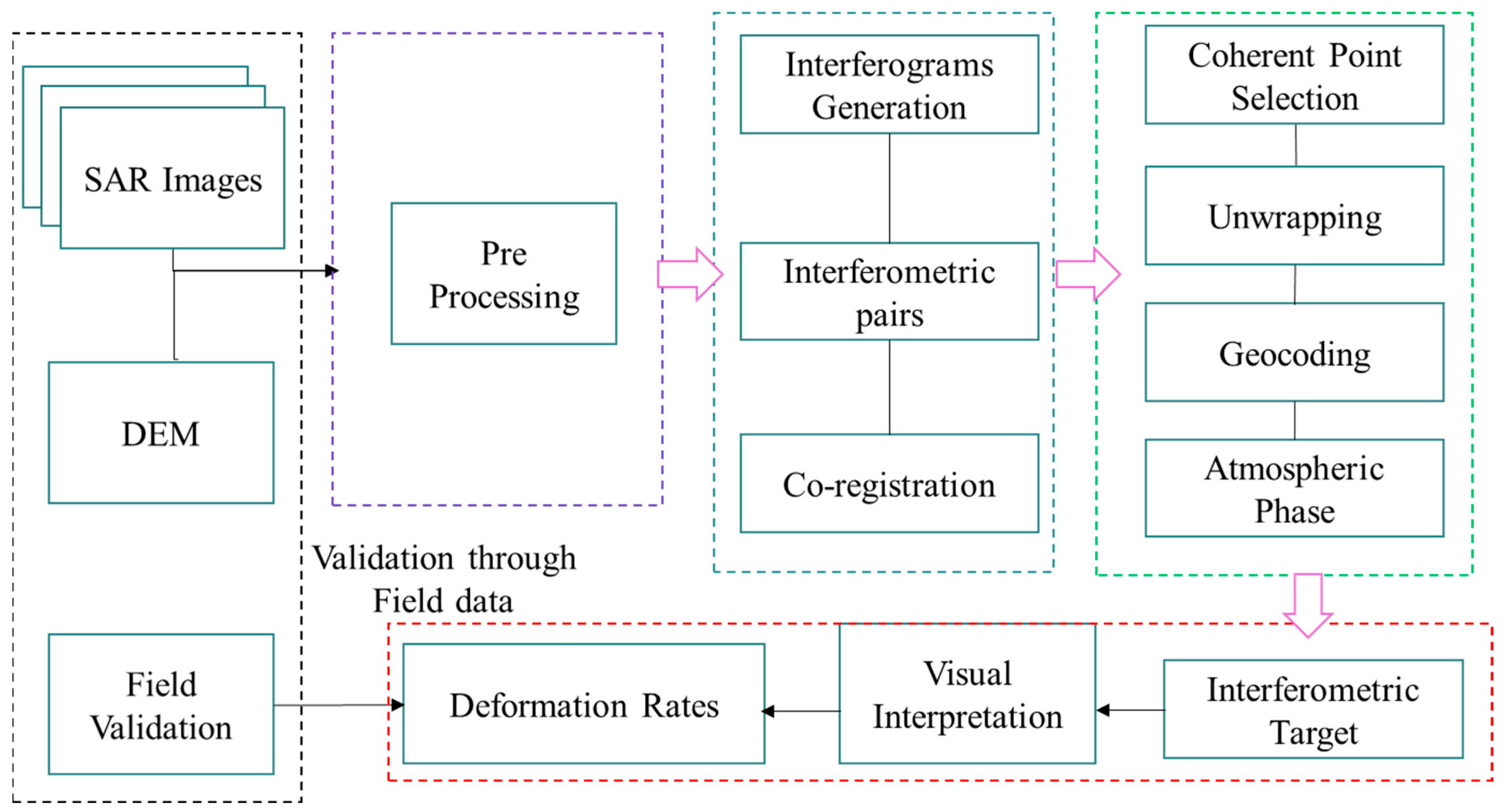
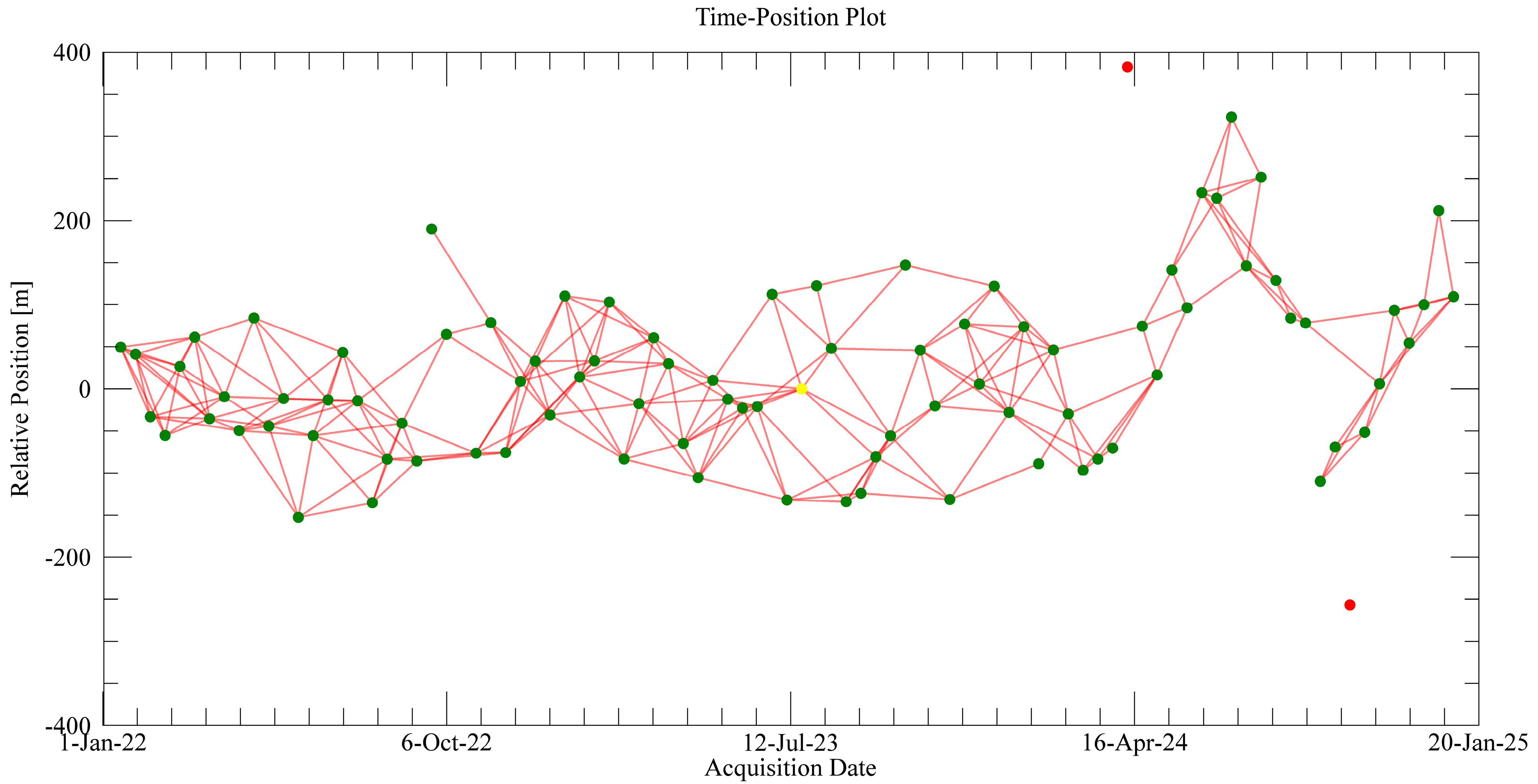
3.1. SBAS-InSAR Processing

The small-baseline subset (SBAS) InSAR technique reliably retrieves surface deformation by stacking high-coherence interferograms. When coherence or stack size is limited, however, precision is reduced and noise levels rise [11,41,42]. Accordingly, SBAS was applied to generate the LOS displacement time series for the Dasu reservoir study area (Figure 4). SBAS processing utilized 92 Sentinel-1 IW SLCs (C-band, VV polarization, ascending orbit, path 100/frame 112), acquired every 12 days from 3 January 2022 to 30 December 2024. All SLCs were co-registered to a 30 m SRTM DEM (ENVI 5.6 + SARScape 5.6.2) and multi-looked (2 × 8 looks) to boost phase SNR. The spatio-temporal baseline is shown in Figure 5. All other acquisitions maintain temporal edges to both preceding and subsequent dates; the 6 October 2022 node is limited to a single link because its mean interferometric coherence matches sufficient coherence with only the 18 October 2022 image, and all other adjacent dates fall below its range. Interferogram pairs satisfying |ΔB⊥| ≤ 2% critical baseline and temporal |Δt| ≤ 72 days yielded 262 interferograms. Each was filtered with a 32-pixel Goldstein scheme and unwrapped using SNAPHU, then inverted via weighted least squares to recover one LOS displacement per acquisition. Quality control (mean coherence < 0.25; residue density > 0.1 cycles km²) discarded noisy dates, leaving 90 valid epochs. A second-order spatial filter removed residual atmospheric artifacts.

3.2. Development of the Proposed Model

3.2.1. Data Collection and Processing

Initially, the spatial baseline and three temporal SAR acquisitions were combined into a unified dataset where each record corresponds to a pixel at acquisition time $t_n\in$ [43]. Further, these geographic features and coordinates are normalized as follows:

$$X_{n^{\prime }}={\displaystyle \frac{X_n-{\mu }_X}{{\sigma }_X}},\hspace{1em}\hspace{1em}{Y}_{n^{\prime }}={\displaystyle \frac{Y_n-{\mu }_Y}{{\sigma }_Y}},$$

(1)

where ${\mu }_X,{\sigma }_X$ and ${\mu }_Y,{\sigma }_Y$ are the empirical means and standard deviations of $X_n$ and $\left\{Y_n\right\}$, respectively. Continuous covariates are clipped at their 1st and 99th percentiles and then standardized. Skewed variables such as rainfall receive a $\mathrm{l}\mathrm{o}\mathrm{g}(1+·)$ transform. We engineer interaction features such as

$$X_{n^{\prime }}{Y}_{n^{\prime }},\hspace{1em}\mathrm{e}\mathrm{l}\mathrm{e}\mathrm{v}\mathrm{a}\mathrm{t}\mathrm{i}\mathrm{o}\mathrm{n}\times \mathrm{s}\mathrm{l}\mathrm{o}\mathrm{p}\mathrm{e},\hspace{1em}\mathrm{s}\mathrm{l}\mathrm{o}\mathrm{p}\mathrm{e}\times \mathrm{r}\mathrm{a}\mathrm{i}\mathrm{n}\mathrm{f}\mathrm{a}\mathrm{l}\mathrm{l},$$

and generate one-hot region embeddings by applying K-means clustering to $(X_{n^{\prime }},Y_{n^{\prime }})$. The acquisition index $t_n$ is encoded cyclically through

$$t_n^{\left(\mathrm{s}\mathrm{i}\mathrm{n}\right)}=\mathrm{s}\mathrm{i}\mathrm{n}\left(2\pi \hspace{0.17em}{t}_n/4\right),\hspace{1em}{t}_n^{\left(\mathrm{c}\mathrm{o}\mathrm{s}\right)}=\mathrm{c}\mathrm{o}\mathrm{s}\left(2\pi \hspace{0.17em}{t}_n/4\right)$$

(2)

All raw and engineered features are concatenated into a single vector ${\mathbf{x}}_n$ and then re-standardized. Observed InSAR displacements $y_n$ are standardized to zero mean and unit variance, where missing values are set to zero, and a binary mask $m_n$ indicates whether $y_n$ is observed. Each node $n$ is thus represented by ${\mathbf{x}}_n$, the standardized target ${\tilde{y}}_n$, and mask $m_n$, providing a complete feature set for subsequent graph construction and modeling.

3.2.2. Spatial–Temporal Graph Construction

Preprocessed pixel-per-map records are represented as graph nodes, and two types of edges are constructed to capture spatio-temporal relationships (Figure 6). For spatial connectivity, it identifies the eight nearest neighbors of node n in three-dimensional space ${X^{՜}}_n$, ${Y^{՜}}_n$, $t_n$ using Euclidean distance. For each neighbor j, this creates a directed edge $n\to j$ with weight

$$w_{nj}^{\left(sp\right)}={\displaystyle \frac{1}{\parallel \left({X^{՜}}_n,{Y^{՜}}_n,t_n\right)-\left({X^{՜}}_j,{Y^{՜}}_j,t_j\right)\parallel 2+\epsilon }}$$

(3)

where $\epsilon ={10}^{-6}$ avoids division by zero.

Temporal continuity is modeled by connecting each node bidirectionally to its counterparts in the previous and next acquisitions, assigning a uniform weight of 1.0 to these edges. Each edge is labeled with a binary “edge-type” indicator “0” for spatial and “1” for temporal, so that the model can apply separate attention mechanisms. Finally, all node feature vectors are aggregated, along with the binary mask indicating which InSAR displacements are observed, edge index pairs, edge weights, and edge-type flags, into a single graph data structure, providing a complete representation for the proposed spatio-temporal D-GAT Imputer.

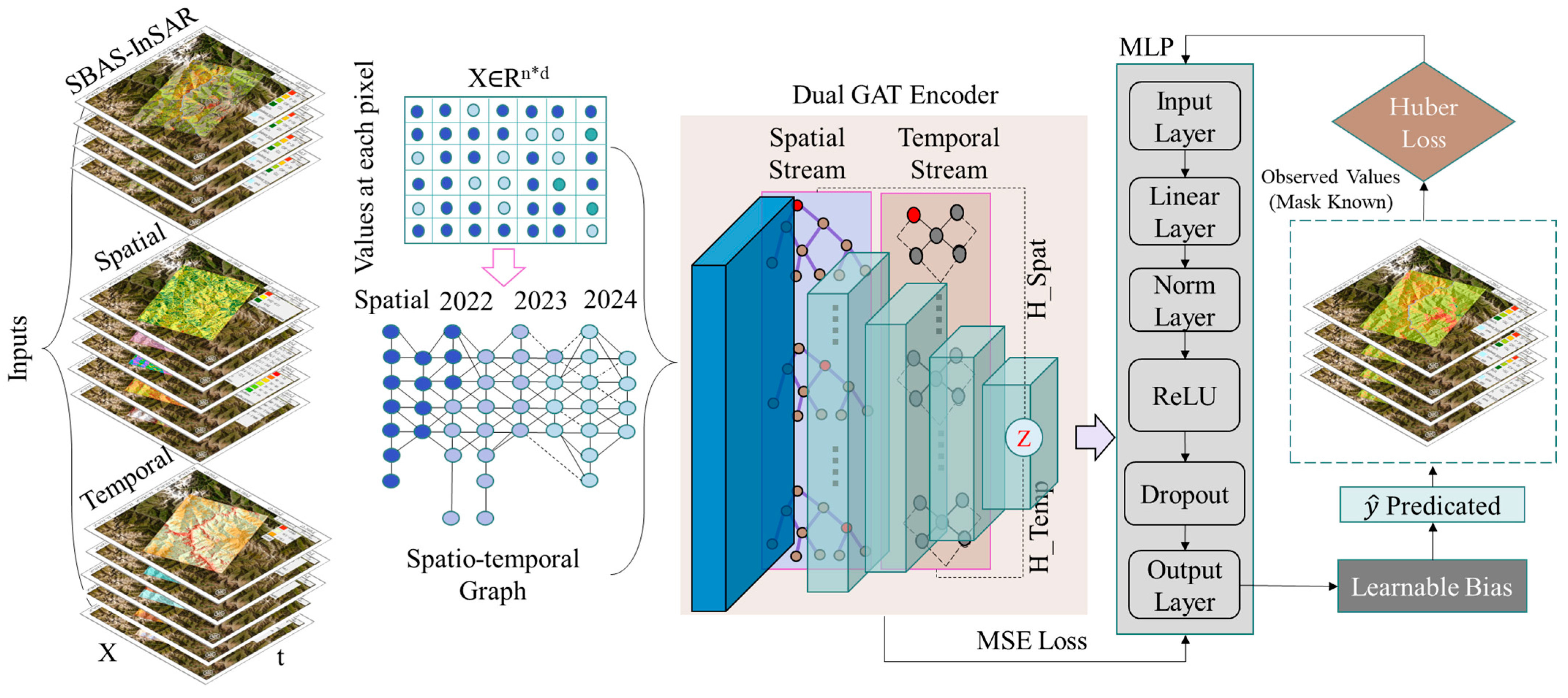
3.2.3. Spatial–Temporal Dual GAT InSAR Deformation Framework (ST D-GAT Framework)

The preprocessed graph is presented by $G=(\mathcal{V},\hspace{0.17em}{\mathcal{E}}_{\mathrm{s}\mathrm{p}}\cup {\mathcal{E}}_{\mathrm{t}\mathrm{m}})$, where each node $i\in \mathcal{V}$ carries a standardized feature vector ${\mathbf{x}}_i\in {\mathbb{R}}^d$, a time index $t_i\in$, and a binary mask $m_i\in \{0,1\}$ indicating whether its InSAR displacement $y_i$ is observed. The model encodes acquisition information using a trainable time-embedding matrix ${\mathbf{E}}^{\left(t\right)}\in {\mathbb{R}}^{4\times 16}$. For node $i$, ${\mathbf{e}}_i^{\left(t\right)}={\mathbf{E}}_{t_i,:}^{\left(t\right)}\in {\mathbb{R}}^{16}$ is extracted and concatenated with ${\mathbf{x}}_i$ to form the initial hidden state

$${\mathbf{h}}_i^{\left(0\right)}=\left[\begin{array}{c}{\mathbf{x}}_i\\ {\mathbf{e}}_i^{\left(t\right)}\end{array}\right]$$

(4)

Next, two spatial attention layers were applied to share information among each node (8 nearest neighbors), where proximity is measured in the normalized $(X^{\prime },Y^{\prime },t)$ coordinate space. At each spatial layer, a learnable linear map ${\mathbf{W}}_{\mathrm{s}\mathrm{p}}^{\left(\mathcal{l}\right)}$ was applied to the previous hidden state ${\mathbf{h}}_i^{(\mathcal{l}-1)}$ which denotes the projected vector by ${\tilde{\mathbf{h}}}_i^{(\mathcal{l}-1)}$, where each neighbor $j\in {\mathcal{N}}_{\mathrm{s}\mathrm{p}}\left(i\right)$ has its own ${\tilde{\mathbf{h}}}_j^{(\mathcal{l}-1)}$, and the spatial edge weight between $i$ and $j$ is

$$w_{ji}^{\left(\mathrm{s}\mathrm{p}\right)}={\displaystyle \frac{1}{‖(X_{j^{\prime }},Y_{j^{\prime }},t_j)-(X_{i^{\prime }},Y_{i^{\prime }},t_i)‖+\epsilon }} \mathrm{w}\mathrm{i}\mathrm{t}\mathrm{h}\hspace{0.17em}\epsilon ={10}^{-6}$$

(5)

Combine these into an “attention logit” for each neighbor pair by passing the concatenation $\left[{\tilde{\mathbf{h}}}_i^{(\mathcal{l}-1)};\hspace{0.17em}{\tilde{\mathbf{h}}}_j^{(\mathcal{l}-1)};\hspace{0.17em}{w}_{ji}^{\left(\mathrm{s}\mathrm{p}\right)}\right]$ through a small vector ${\mathbf{a}}_{\mathrm{s}\mathrm{p}}^{\left(\mathcal{l}\right)}$ and a LeakyReLU. Normalizing these logits’ overall spatial neighbors of $i$ yields attention weights ${\alpha }_{ji}^{\left(\mathcal{l}\right)},$ and node $i$ then aggregates

$${\mathbf{m}}_i^{\left(\mathcal{l}\right)}={\sum }_{j\in {\mathcal{N}}_{\mathrm{s}\mathrm{p}}\left(i\right)}{\alpha }_{ji}^{\left(\mathcal{l}\right)}\hspace{0.17em}{\tilde{\mathbf{h}}}_j^{(\mathcal{l}-1)}$$

(6)

Then, an ELU activation adds the residual ${\tilde{\mathbf{h}}}_i^{(\mathcal{l}-1)}$, and layer-normalizes to get ${\mathbf{h}}_i^{\left(\mathcal{l}\right)}$. After two spatial layers, the resulting “spatial embedding” is

$${\mathbf{z}}_i={\mathbf{h}}_i^{\left(2\right)}$$

The two temporal attention layers were then applied to share information across time for each pixel. Initialize ${\mathbf{g}}_i^{\left(0\right)}={\mathbf{z}}_i$ at each temporal layer, the first project ${\mathbf{g}}_i^{(\mathcal{l}-1)}$ via ${\mathbf{W}}_{\mathrm{t}\mathrm{m}}^{\left(\mathcal{l}\right)}$, yielding ${\tilde{\mathbf{g}}}_i^{(\mathcal{l}-1)}$. Since each temporal edge has weight 1, for each time-neighbor $j\in {\mathcal{N}}_{\mathrm{t}\mathrm{m}}\left(i\right),$ which computes a logit bypassing $\left[{\tilde{\mathbf{g}}}_i^{(\mathcal{l}-1)};\hspace{0.17em}{\tilde{\mathbf{g}}}_j^{(\mathcal{l}-1)};\hspace{0.17em}1\right]$ through ${\mathbf{a}}_{\mathrm{t}\mathrm{m}}^{\left(\mathcal{l}\right)}$ and LeakyReLU. After softmax normalization, we obtain ${\beta }_{ji}^{\left(\mathcal{l}\right)}$, node $i$ aggregates

$${\mathbf{n}}_i^{\left(\mathcal{l}\right)}={\sum }_{j\in {\mathcal{N}}_{\mathrm{t}\mathrm{m}}\left(i\right)}{\beta }_{ji}^{\left(\mathcal{l}\right)}{\tilde{\mathbf{g}}}_j^{(\mathcal{l}-1)}$$

(7)

where applied ELU adds the residual ${\tilde{\mathbf{g}}}_i^{(\mathcal{l}-1)}$, and layer-normalizes to get ${\mathbf{g}}_i^{\left(\mathcal{l}\right)}$. After two temporal layers, the final “temporal embedding” is

$${\mathbf{g}}_i={\mathbf{g}}_i^{\left(2\right)}$$

then fuse the spatial and temporal embeddings simply by addition:

$${\mathbf{h}}_i^{\left(\mathrm{f}\mathrm{i}\mathrm{n}\mathrm{a}\mathrm{l}\right)}={\mathbf{z}}_i+{\mathbf{g}}_i$$

A two-layer MLP then maps ${\mathbf{h}}_i^{\left(\mathrm{f}\mathrm{i}\mathrm{n}\mathrm{a}\mathrm{l}\right)}$ to a single standardized output ${\widehat{y}}_i^{\left(\mathrm{s}\mathrm{p}\right)}$. Specifically,

$${\mathbf{u}}_i=\mathrm{R}\mathrm{e}\mathrm{L}\mathrm{U}\left({\mathbf{W}}_1{\mathbf{h}}_i^{\left(\mathrm{f}\mathrm{i}\mathrm{n}\mathrm{a}\mathrm{l}\right)}+{\mathbf{b}}_1\right),\hspace{1em}{\widehat{y}}_i^{\left(\mathrm{s}\mathrm{p}\right)}={\mathbf{w}}_2^T{\mathbf{u}}_i+b_2$$

(8)

where ${\mathbf{W}}_1\in {\mathbb{R}}^{64\times 128}$, ${\mathbf{b}}_1\in {\mathbb{R}}^{64}$, ${\mathbf{w}}_2\in {\mathbb{R}}^{64}$, and $b_2\in \mathbb{R}$. To correct for per-map artifacts such as atmospheric noise, a learnable bias ${\beta }_{t_i}$ was introduced for each map $t_i$ and added.

$${\widehat{y}}_i={\widehat{y}}_i^{\left(\mathrm{s}\mathrm{p}\right)}+{\beta }_{t_i}.$$

Finally, conversion to original units is performed by

$${\widehat{y}}_i^{\left(\mathrm{o}\mathrm{r}\mathrm{i}\mathrm{g}\right)}={\widehat{y}}_i\hspace{0.17em}{\sigma }_y+{\mu }_y,$$

(9)

where ${\mu }_y$ and ${\sigma }_y$ are the mean and standard deviation of all observed displacements $\{y_i:m_i=1\}$.

In training, all the parameters, such as the time embeddings ${\mathbf{E}}^{\left(t\right)}$, attention weights $\{{\mathbf{W}}_{\mathrm{s}\mathrm{p}}^{\left(\mathcal{l}\right)},{\mathbf{a}}_{\mathrm{s}\mathrm{p}}^{\left(\mathcal{l}\right)},{\mathbf{W}}_{\mathrm{t}\mathrm{m}}^{\left(\mathcal{l}\right)},{\mathbf{a}}_{\mathrm{t}\mathrm{m}}^{\left(\mathcal{l}\right)}$ MLP weights ${\mathbf{W}}_1,{\mathbf{b}}_1,{\mathbf{w}}_2,b_2$, and map biases $\mathbf{\beta }$ are trained by minimizing the Huber loss over observed nodes:

$${\mathcal{l}}_{\delta }({\widehat{y}}_i,{\tilde{y}}_i)=\left\{\begin{array}{ll}1/2({\widehat{y}}_i-{\tilde{y}}_i{)}^2,& |{\widehat{y}}_i-{\tilde{y}}_i|\le 1,\\ |{\widehat{y}}_i-{\tilde{y}}_i|-1/2,& |{\widehat{y}}_i-{\tilde{y}}_i|>1,\end{array}\right.\hspace{1em}\mathcal{L}={\displaystyle \frac{1}{{\sum }_i{m}_i}}\sum _i{m}_i{\mathcal{l}}_1\left({\widehat{y}}_i,{\tilde{y}}_i\right)$$

(10)

where ${\tilde{y}}_i=(y_i-{\mu }_y)/{\sigma }_y$ if $m_i=1$, and 0 otherwise. The model is optimized with Adam (weight decay ${10}^{-5}$) with a OneCycleLR schedule over 600 epochs in mixed precision, applying early stopping based on map-stratified validation ${\mathrm{R}}^2$. This approach yields smooth, gap-free InSAR deformation maps that facilitate continuous landslide monitoring and robust modeling.

3.3. Evaluation and Validation of the Model

Model validation is carried out on the 20% subset of SBAS-InSAR observations that was held out during training. These LOS displacement values provide the ground truth for all quantitative metrics (RMSE, MAE, Bias, R², and Pearson’s ρ). The documented landslide inventory is reserved for the qualitative comparison presented in Section 4.

Following training, the model loads its best checkpoint and produces standardized predictions, ${\widehat{y}}_i$ for every node $i$. They are transformed back into actual deformation measurements using the original mean and standard deviation:

$${\widehat{y}}_i^{\left(\mathrm{o}\mathrm{r}\mathrm{i}\mathrm{g}\right)}={\widehat{y}}_i{\sigma }_y+{\mu }_y$$

(11)

where ${\mu }_y$ and ${\sigma }_y$ denote the mean and standard deviation of all observed InSAR displacements. For each node $i$ with $m_i=1$, we then compare ${\widehat{y}}_i^{\left(\mathrm{o}\mathrm{r}\mathrm{i}\mathrm{g}\right)}$ against the true value $y_i$ and compute the following error metrics:

Root Mean Squared Error (RMSE):

$$\mathrm{R}\mathrm{M}\mathrm{S}\mathrm{E}=\sqrt{{\displaystyle \frac{1}{N_{\mathrm{o}\mathrm{b}\mathrm{s}}}}{\sum }_{i:m_i=1}({\widehat{y}}_i^{\left(\mathrm{o}\mathrm{r}\mathrm{i}\mathrm{g}\right)}-y_i{)}^2}$$

(12)

where $N_{\mathrm{o}\mathrm{b}\mathrm{s}}={\sum }_i{m}_i$.

Mean Absolute Error (MAE):

$$\mathrm{M}\mathrm{A}\mathrm{E}={\displaystyle \frac{1}{N_{\mathrm{o}\mathrm{b}\mathrm{s}}}}{\sum }_{i:m_i=1}|{\widehat{y}}_i^{\left(\mathrm{o}\mathrm{r}\mathrm{i}\mathrm{g}\right)}-y_i|$$

(13)

Bias:

$$\mathrm{B}\mathrm{i}\mathrm{a}\mathrm{s}={\displaystyle \frac{1}{N_{\mathrm{o}\mathrm{b}\mathrm{s}}}}{\sum }_{i:m_i=1}\left({\widehat{y}}_i^{\left(\mathrm{o}\mathrm{r}\mathrm{i}\mathrm{g}\right)}-y_i\right)$$

(14)

Coefficient of Determination (${\mathrm{R}}^2$):

$${\mathrm{R}}^2=1-{\displaystyle \frac{{\sum }_{i:m_i=1}({\widehat{y}}_i^{\left(\mathrm{o}\mathrm{r}\mathrm{i}\mathrm{g}\right)}-y_i{)}^2}{{\sum }_{i:m_i=1}(y_i-\overline{y}{)}^2}},\hspace{1em}\overline{y}={\displaystyle \frac{1}{N_{\mathrm{o}\mathrm{b}\mathrm{s}}}}{\sum }_{i:m_i=1}{y}_i$$

(15)

Pearson’s Correlation ($\rho$):

$$\rho ={\displaystyle \frac{{\sum }_{i:m_i=1}\left(y_i-\overline{y}\right)\left({\widehat{y}}_i^{\left(\mathrm{o}\mathrm{r}\mathrm{i}\mathrm{g}\right)}-\overline{\widehat{y}}\right)}{\sqrt{{\sum }_{i:m_i=1}(y_i-\overline{y}{)}^2}\hspace{0.33em}\sqrt{{\sum }_{i:m_i=1}({\widehat{y}}_i^{\left(\mathrm{o}\mathrm{r}\mathrm{i}\mathrm{g}\right)}-\overline{\widehat{y}}{)}^2}}}$$

(16)

where $\overline{\widehat{y}}={\displaystyle \frac{1}{N_{\mathrm{o}\mathrm{b}\mathrm{s}}}}{\sum }_{i:m_i=1}{\widehat{y}}_i^{\left(\mathrm{o}\mathrm{r}\mathrm{i}\mathrm{g}\right)}$.

Each metric is computed both globally (overall $i$ with $m_i=1$) and map-wise, by restricting the summations to nodes satisfying $m_i=1$ and $t_i=s$ for each $s\in \{0,1,2,3\}$. This map-specific evaluation reveals the presence of any temporal variation in imputation accuracy. Convergence and generalization are evaluated through plotting of both training and validation Huber loss across all epochs, supplemented by corresponding ${\mathrm{R}}^2$ curves to illustrate performance improvements over time. The analysis also performed map-specific validation, including R² trajectories and ROC curves for all four maps, which revealed spatio-temporal patterns that highlighted model precision and robustness. Finally, for each map, scatter plots of $y_i$ versus ${\widehat{y}}_i^{\left(\mathrm{o}\mathrm{r}\mathrm{i}\mathrm{g}\right)}$ and the imputed deformation maps were plotted. Together, these numerical and graphical diagnostics confirm that the model reliably fills missing InSAR values and produces continuous deformation fields suitable for geohazard assessment and landslide monitoring.

4. Results

4.1. SBAS-InSAR Analysis

SBAS-InSAR processing analyzed detailed deformation spatio-temporal and corresponding coherence-based void masks, providing the foundational data for the gap-filling analysis. Deformation statistics and void-mask fractions were computed directly from the SBAS time series, and spatial patterns were visualized on a 30 m grid. The SBAS-InSAR LOS displacement maps consist of one static baseline map and three annual maps for 2022, 2023, and 2024. The baseline map shows values from −176 to 133 mm/y; the 2022 map ranges from −58 to 41 mm/y; the 2023 map from −119 to 71 mm/y; and the 2024 map from −237 to 132 mm/y (Figure 7). The positive LOS values have been inverted to represent downslope displacement (i.e., movement away from the satellite), making subsidence appear as positive deformation for easier interpretation. Slopes on the river’s right bank, especially those 3 to 7 km downstream of the reservoir, showed high LOS displacement magnitudes, indicating active downslope movement. Many areas on the left bank, most notably the Uchar debris flow site (which experienced two significant monsoon failures in 2022) and the Kaigha slope toe failure along the Karakoram Highway, lacked valid InSAR measurements due to severe layover, shadowing, and temporal decorrelation. Other potentially unstable slopes in this zone were similarly unobserved for the same reasons. Across all LOS maps, approximately 48% of pixels are voids, with nearly 20% concentrated along the right bank near the Dasu dam. These spatial and temporal gap patterns underscore the necessity of the imputation framework to recover the full deformation history.

4.2. ST D-GAT InSAR Imputation Performance

The ST D-GAT Framework was applied to reconstruct missing LOS displacement values from SBAS-InSAR data affected by coherence loss, radar geometry, and seasonal decorrelation. The dataset comprises four SAR acquisitions, including a static spatial baseline and annual InSAR maps from 2022 to 2024. In total, approximately 48% of the pixel-time records were unavailable in each raw SBAS stack (Figure 7 and Figure 8, respectively). The ST D-GAT framework encodes the whole dataset as a single spatio-temporal graph, where each node represents a pixel at a specific time of SAR acquisition. Spatial edges connect a pixel to its nearest neighbors within the same date, while temporal edges link the exact location across consecutive years. This graph structure enables the model to propagate information from known deformation values and treat them as control points, filling in surrounding missing regions, guided by learned terrain and temporal features.

The model is trained using the observed SBAS-InSAR LOS values. During learning, it differentiates between known and missing pixels by masking the loss function, ensuring that only reliable data contributes to parameter updates. Each node is enriched with a feature vector that combines spatial coordinates, environmental covariates (e.g., slope, rainfall), temporal encodings, and spatial cluster embeddings, which guide the model in identifying deformation patterns even where values are missing. The output is a set of imputed values that align perfectly with observed data while extending smoothly into previously void areas. Following imputation, the spatial baseline map, which ranged from −269 mm to 153 mm, was completed with continuous values across the entire reservoir. Similar improvements are observed in the 2022 (−81 to 49 mm), 2023 (−170 to 95 mm), and 2024 (−237 to 132 mm) maps. Key missing regions, such as the Kaigha slope along the Karakoram Highway and the Uchar debris flow site, were filled with plausible deformation values, preserving both spatial trends and interannual displacement continuity. This ensures that even zones with no original LOS values can now be interpreted for hazard analysis. Figure 8 (only imputed pixels) and Figure 9 (complete) illustrate the reconstructed LOS maps, clearly showing improved continuity and deformation consistency. The imputation preserved known values at control points and propagated physically consistent estimates into previously missed zones, validating the model’s ability to infer spatio-temporal ground motion patterns.

4.3. Model Validation and Performance Assessment

A spatio-temporal validation protocol was applied, utilizing 80% of pixels for training and reserving 20% per map for testing, to assess ST D-GAT via regression metrics (RMSE, bias, ρ, R²) and classification performance (ROC-AUC). Results demonstrate robust performance with an overall 0.907 (R²) and 0.947 (ρ), confirming strong signal capture. At the same time, map-specific analysis reveals that the spatial data achieve an R² of 0.914 with an RMSE of 12.066, and temporal maps maintain R² values ranging from 0.807 to 0.897 (Figure 10 and

Table 1. Validation of the ST D-GAT framework.

Method	Maps/Outputs	RMSE	Bias	ρ	R2
ST-GAT	Overall	9.263	—	0.9474	0.907
	Spatial	12.066	0.059	0.951	0.914
	2022	5.782	–0.151	0.887	0.807
	2023	8.027	–0.088	0.935	0.894
	2024	9.990	–0.047	0.942	0.897

and

Table 2. Overall validation of baseline models.

Method	Maps/Outputs	RMSE	ρ	R2
MLP Regressor	Overall	14.626	0.865	0.743
Simple NN	Overall	15.595	0.502	0.735
IDW (K = 8)	Overall	20.020	0.733	0.519
KNN Regressor	Overall	16.543	0.819	0.672
Random Forest	Overall	12.753	0.897	0.805
XGBoost	Overall	14.544	0.866	0.746

). The ROC-AUC remains exceptionally high across all validation sets of the maps (0.91 to 0.96). ST D-GAT delivers strong imputation accuracy across all outputs, consistent with recent deep learning InSAR gap-filling and forecasting studies [43,44]. The Huber Loss and true vs. predicted values were plotted as shown in Figure 11 and Figure 12. These results underscore the effectiveness of ST D-GAT for continuous, high-resolution landslide monitoring in regions challenged by decorrelation and missing data.

4.4. Baseline Models

A set of six widely used baseline models was evaluated on the same validation data to benchmark ST D-GAT’s performance. These include geostatistical and machine learning approaches, such as Inverse Distance Weighting (IDW), K-Nearest Neighbors Regressor (KNN), Random Forest (RF), XGBoost, Multi-Layer Perceptron (MLP), and neural network (NN). All baselines used the same feature vectors constructed from spatial–temporal covariates and terrain factors. Table 2 and

Table 3. Spatio-temporal validation of baseline models.

Method	Maps/Outputs	RMSE	Bias	ρ	R2
MLP Regressor	Spatial	19.989	0.324	0.863	0.738
	2022	8.301	0.098	0.771	0.561
	2023	12.448	0.064	0.838	0.697
	2024	15.240	–0.056	0.862	0.736
Simple NN	Spatial	21.885	0.406	0.830	0.725
	2022	10.079	0.011	0.728	0.490
	2023	13.267	0.050	0.818	0.609
	2024	16.801	0.081	0.797	0.704
IDW (K = 8)	Spatial	26.685	16.714	0.911	0.533
	2022	20.658	–3.308	0.793	–1.719
	2023	16.814	–11.818	0.884	0.446
	2024	13.479	0.171	0.903	0.794
KNN Regressor	Spatial	22.939	3.238	0.813	0.655
	2022	8.838	–0.505	0.733	0.502
	2023	13.596	–1.770	0.803	0.638
	2024	17.476	–1.199	0.810	0.653
Random Forest	Spatial	18.234	0.051	0.884	0.782
	2022	5.937	–0.171	0.881	0.775
	2023	9.736	–0.257	0.903	0.814
	2024	13.712	0.104	0.888	0.786
XGBoost	Spatial	20.040	0.284	0.864	0.736
	2022	7.679	–0.101	0.796	0.624
	2023	11.758	–0.364	0.855	0.729
	2024	15.727	–0.012	0.849	0.719

present the validation performance of baseline models. Random Forest achieved the highest R² (0.805), followed by XGBoost (0.746) and MLP (0.743). IDW performed poorly with R² = 0.519 despite a high Pearson correlation (0.733) due to a significant spatial bias and an inability to account for contextual features.

Per-map analysis revealed that most models performed best, with the Random Forest model achieving an RMSE of 5.937 mm and an R² of 0.775. However, baseline models struggled with consistency across all years. For example, KNN showed a strong spatial correlation (0.813) but introduced higher bias across 2023–2024 maps. IDW exhibited extreme outliers, particularly in 2022 (Bias = −3.3, and R² = −1.719), highlighting its limitations in temporally variable terrain. In contrast, ST D-GAT achieved an overall RMSE of 9.263 mm and R² of 0.907. In each spatio-temporal output, the performance remained strong, with R² of 0.914, 0.807, 0.894, 0.897, and RMSEs of 12.066, 5.782, 8.027, and 9.990 (spatial, 2022, 2023, and 2024), respectively. These results surpass all baselines, demonstrating that ST D-GAT consistently achieves low errors and high R² values across every map. This confirms the advantage of combining explicit spatio-temporal modeling with map-specific bias correction for InSAR imputation.

4.5. Ablation Analysis

A series of controlled analyses were conducted to quantify how each component of the ST D-GAT framework contributes to overall performance (

Table 4. Ablation analysis of the proposed model.

Variant	Val R2	RMSE	Spatial R2	2022 R2	2023 R2	2024 R2
Full Model	0.929	8.85	0.937	0.826	0.918	0.922
Spatial-Only GAT (No Temp)	0.776	12.24	0.821	0.642	0.715	0.704
Temporal-Only GAT (No Spatial)	0.702	14.12	0.153	0.673	0.708	0.695
No Engineered Features	0.839	10.38	0.874	0.752	0.817	0.805
No Slice-Bias Head	0.912	9.72	0.928	0.794	0.881	0.872

). All ablation variants used the same data splits, hyperparameters, and preprocessing steps as the whole model. Turning off the two temporal GAT Conv layers, such as setting the temporal embedding to zero after the spatial stream, yielded a Spatial-Only GAT variant. In this case, overall validation ${\mathrm{R}}^2$ dropped from 0.929 to 0.776, and RMSE rose from 8.85 to 12.24. Map-wise ${\mathrm{R}}^2$ values on (spatial, 2022, 2023, 2024) fell to (0.821, 0.642, 0.715, 0.704). Removing the two spatial GAT Conv layers instead, where the initial concatenated features are directly fed into the temporal stream, produced a temporal-only GAT variant. Without spatial message passing, overall ${\mathrm{R}}^2$ fell further to 0.702, and RMSE increased to 14.12, with map-wise ${\mathrm{R}}^2$ of (0.153, 0.673, 0.708, 0.695), respectively. This confirms that local spatial context is essential for reconstructing the baseline map and for accurate imputation. Similarly, after retaining both GAT streams with disabled engineered features (interaction terms, log-transforms, and spatial clustering), overall ${\mathrm{R}}^2$ fell to 0.839, and RMSE increased to 10.38. Corresponding ${\mathrm{R}}^2$ values are dropped to approximately (0.874, 0.752, 0.817, 0.805), indicating that nonlinear covariates and cluster embeddings significantly enhance accuracy. Finally, the impact of the slice-bias head was evaluated by setting all bias parameters ${\beta }_s=0$. Although the overall validation ${\mathrm{R}}^2$ decreased only modestly from 0.929 to 0.912, map-wise ${\mathrm{R}}^2$ values fall to (0.928, 0.794, 0.881, 0.872), demonstrating that learning per-map offsets further refines predictions. Together, these results confirm that spatial GAT, temporal GAT, feature engineering, and map-bias correction contribute meaningful contributions to the final imputation accuracy.

5. Discussion

This study presents a hybrid spatio-temporal Graph Attention framework (ST D-GAT) to impute missing InSAR line-of-sight (LOS) deformation values in challenging mountainous terrain, such as the Dasu reservoir region (Kohistan, Pakistan). The proposed model leverages both observed InSAR displacements and influential geospatial information to reconstruct deformation patterns with high accuracy and spatial continuity. It also models the spatial and temporal dependencies that drive slope behavior [33,45,46], offering a more physically consistent reconstruction of ground motion. Post-imputation analysis identified previously undetected critical sites validated against field observations (Figure 13) and quantified their spatio-temporal displacement trends along Dasu Reservoir (Figure 14).

One notable aspect of the ST D-GAT framework is its integration of comprehensive geospatial covariates. In total, 14 spatial factors were incorporated to represent long-term ground deformation, including terrain morphology, geological structures, hydrology, and surface cover. These variables were validated in global landslide studies [47,48]. Temporal factors (10 dynamic layers) capture environmental fluctuations from 2022 to 2024, including precipitation, temperature, soil moisture, evapotranspiration, and vegetation indices. These time-varying inputs offer insight into short-term triggers, such as monsoon storms, aligning with slope hydromechanics research [49,50]. The model integrates these spatio-temporal covariates in a unified dual-GAT architecture. Spatial attention modules enable each node to incorporate contextual signals from nearby terrain, while temporal attention layers capture the evolution of displacement across SAR acquisitions, overcoming the limitations of irregular grid structures in CNN-based approaches [51]. This design directly addresses deficiencies in classical geostatistical methods, such as Kriging, which neglects deformation history and outperforms patch-based CNNs that struggle with SBAS data geometry.

The validation results demonstrate that the ST D-GAT framework effectively captures both the magnitude and spatio-temporal trend of InSAR LOS deformation patterns, even in areas affected by radar decorrelation and shadowing. Using a map-wise holdout strategy (20% per map), the model achieved an overall R² of 0.907 and a Pearson’s correlation coefficient (ρ) of 0.947, indicating a strong match between predicted and observed values across spatial and temporal maps. Similarly, RMSE values demonstrated the reliability and high performance of the model in both spatial and temporal maps [52]. Notably, the model also maintained low bias (–0.15 to 0.05), reinforcing its capacity to avoid systematic over- or underestimation during imputation. Furthermore, ROC-AUC scores greater than 0.91 across all validation sets support the model’s reliability and high accuracy [30,53]. These results outperform widely used machine learning and deep learning baselines, such as MLP (R² of 0.743), Random Forest (R² of 0.805), and XGBoost (R² of 0.746). Compared to previous research, the ST D-GAT framework builds upon and complements a growing body of work that integrates InSAR data with deep learning for landslide monitoring. For example, Tian and Zhang [27] enabled refined susceptibility mapping through MT-InSAR and SVM fusion; Dun and Feng [28] and Zhengrong and Wenfei [29] decoded deformation mechanisms in reservoir slopes; Chang and Dong [30] modeled 3D displacements via topography-constrained strain; while Aswathi and Kumar [31] and Miller and Pelletier [32] comprehensively reviewed InSAR-based deep learning progress for landslide monitoring.

Building on the foundation of the InSAR-based deep learning approach, the ST D-GAT framework delivers key advantages for landslide monitoring. First, it represents the entire SBAS time series as a single graph: each node (a pixel on a given acquisition date) is linked spatially to its nearest neighbors and temporally to itself in adjacent dates, ensuring that coherent deformation signals flow through complex terrain. Second, separate Graph Attention streams learn spatial terrain-driven controls within each acquisition and temporal annual displacement trends before fusing their outputs. Third, a compact MLP with per-map bias terms corrects systematic artifacts (e.g., atmospheric delays) and produces final, LOS estimates. Despite its strong performance, ST D-GAT remains a predictive model rather than a direct measurement: its imputed values are best interpreted as informed estimates, not exact ground truth. The need to build and train graphs with over a million nodes also imposes substantial computational and memory demands. Finally, this study did not have access to continuous ground-based displacement records in the steep, inaccessible terrain of the Dasu region. Incorporating high-precision GPS, extensometer, or tilt-meter data, as well as leveraging higher-revisit SAR and in situ hydrological or meteorological sensors, would further tighten the link between model predictions and actual slope behavior. Extending ST D-GAT to other reservoir-induced landslide settings will also help assess its generality and operational readiness for near-real-time hazard monitoring.

6. Conclusions

This study presents a novel approach in which missing InSAR values are imputed from known InSAR pixels augmented with 24 deformation-influential variables within a hybrid spatio-temporal Dual Graph Attention Network (ST D-GAT) framework. The model is then applied to the Dasu reservoir region (Kohistan, Pakistan). Initial SBAS-InSAR analysis revealed that approximately 48% of LOS pixel-time observations were missing, primarily due to terrain-induced radar distortion and temporal decorrelation. Notably, nearly 20% of these voids were located along the riverbanks close to the reservoir. Encoding the SBAS-InSAR time series as a unified spatio-temporal graph and integrating multiple geospatial and environmental inputs enables the accurate reconstruction of deformation patterns, even in areas affected by radar decorrelation, layover, or seasonal coherence loss. The main findings are as follows:

• By incorporating 14 spatial and 10 temporal predictors (encompassing topographic, geological, hydrological, climatic, anthropogenic, hazard, vegetation, and soil factors) with SBAS-InSAR results, the model identifies both long-term susceptibility and short-term triggers, enabling it to impute realistic deformation even where InSAR measurements are unavailable.
• The framework successfully filled voids in geologically critical areas, such as the Uchar debris-flow site and Kaigha slope, ensuring temporal continuity and preserving observed deformation trends. This is essential for early warning systems and hazard assessment in areas where a high number of InSAR pixels are missing.
• The model achieved an overall R² of 0.907 and a Pearson’s ρ of 0.947, outperforming classical and machine learning baselines across both spatial and temporal maps. Its ability to reconstruct nearly half of the missing data demonstrates strong generalization under extreme decorrelation.

In conclusion, these imputed LOS displacements are model-based estimates rather than direct measurements; nevertheless, their close agreement with known SBAS values and field-verified landslides shows that they provide reliable, actionable insights. By bridging the gaps in SAR coverage, ST D-GAT enables near-continuous deformation monitoring and offering hazard managers and engineers a powerful tool for planning, risk assessment, and early warning in steep, vegetation-covered, or infrastructure-sensitive terrain.

References

1. Varnes, D.J. Slope movement types and processes. Spec. Rep. 1978, 176, e33. [Google Scholar]
2. Hungr, O.; Leroueil, S.; Picarelli, L. The Varnes classification of landslide types, an update. Landslides 2014, 11, 167–194. [Google Scholar] [CrossRef]
3. Cruden, D.M.; Varnes, D.J. Landslide types and processes. Landslides Investig. Mitig. Spec. Rep. 1996, 247, 36–75. [Google Scholar]
4. Paronuzzi, P.; Rigo, E.; Bolla, A. Influence of filling–drawdown cycles of the Vajont reservoir on Mt. Toc slope stability. Geomorphology 2013, 191, 75–93. [Google Scholar] [CrossRef]
5. Xu, Z.; Song, S.; Wu, F.; Cao, C.; Ma, M.; Wang, S. Research on the spatiotemporal evolution of deformation and seismic dynamic response characteristics of high-steep loess slope on the northeast edge of the Qinghai-Tibet Plateau. Bull. Eng. Geol. Environ. 2025, 84, 21. [Google Scholar] [CrossRef]
6. Li, L.; Yao, X.; Wen, B.; Zhou, Z.; Li, R. The long-term failure processes of a large reactivated landslide in the Xiluodu reservoir area based on InSAR technology. Front. Earth Sci. 2023, 10, 1055890. [Google Scholar] [CrossRef]
7. Liu, M.; Yang, Z.; Xi, W.; Guo, J.; Yang, H. InSAR-based method for deformation monitoring of landslide source area in Baihetan reservoir, China. Front. Earth Sci. 2023, 11, 1253272. [Google Scholar] [CrossRef]
8. Tang, H.; Wasowski, J.; Juang, C.H. Geohazards in the three Gorges Reservoir Area, China–Lessons learned from decades of research. Eng. Geol. 2019, 261, 105267. [Google Scholar] [CrossRef]
9. Wang, Y.; Dong, J.; Zhang, L.; Deng, S.; Zhang, G.; Liao, M.; Gong, J. Automatic detection and update of landslide inventory before and after impoundments at the Lianghekou reservoir using Sentinel-1 InSAR. Int. J. Appl. Earth Obs. Geoinf. 2023, 118, 103224. [Google Scholar] [CrossRef]
10. Siddique, A.; Tan, Z.; Tan, N.; Ahmad, H.; Li, J.; Liu, J.; Khurram, S.H.; Jiang, Y.; Zeng, N. Remote Sensing and Numerical Simulation for Slope Stability in Open-Pit Mining: Case Study of Sijiaying Iron Ore Mine, China. Geotech. Geol. Eng. 2025, 43, 290. [Google Scholar] [CrossRef]
11. Berardino, P.; Fornaro, G.; Lanari, R.; Sansosti, E. A new algorithm for surface deformation monitoring based on small baseline differential SAR interferograms. IEEE Trans. Geosci. Remote Sens. 2002, 40, 2375–2383. [Google Scholar] [CrossRef]
12. Lanari, R.; Mora, O.; Manunta, M.; Mallorquí, J.J.; Berardino, P.; Sansosti, E. A small-baseline approach for investigating deformations on full-resolution differential SAR interferograms. IEEE Trans. Geosci. Remote Sens. 2004, 42, 1377–1386. [Google Scholar] [CrossRef]
13. Zhang, R.; Zhang, L.; Fang, Z.; Oguchi, T.; Merghadi, A.; Fu, Z.; Dong, A.; Dou, J. Interferometric synthetic aperture Radar (InSAR)-based absence sampling for machine-learning-based landslide susceptibility mapping: The Three Gorges Reservoir area, China. Remote Sens. 2024, 16, 2394. [Google Scholar] [CrossRef]
14. Mondini, A.C.; Guzzetti, F.; Chang, K.-T.; Monserrat, O.; Martha, T.R.; Manconi, A. Landslide failures detection and mapping using Synthetic Aperture Radar: Past, present and future. Earth-Sci. Rev. 2021, 216, 103574. [Google Scholar] [CrossRef]
15. Dai, M.; Li, H.; Long, B.; Wang, X. Quantitative identification of landslide hazard in mountainous open-pit mining areas combined with ascending and descending orbit InSAR technology. Landslides 2024, 21, 2975–2991. [Google Scholar] [CrossRef]
16. Xiong, Z.; Zhang, M.; Ma, J.; Xing, G.; Feng, G.; An, Q. InSAR-based landslide detection method with the assistance of C-index. Landslides 2023, 20, 2709–2723. [Google Scholar] [CrossRef]
17. Dong, J.; Niu, R.; Li, B.; Xu, H.; Wang, S. Potential landslides identification based on temporal and spatial filtering of SBAS-InSAR results. Geomat. Nat. Hazards Risk 2023, 14, 52–75. [Google Scholar] [CrossRef]
18. Torre, D.; Galve, J.P.; Reyes-Carmona, C.; Alfonso-Jorde, D.; Ballesteros, D.; Menichetti, M.; Piacentini, D.; Troiani, F.; Azañón, J.M. Geomorphological assessment as basic complement of InSAR analysis for landslide processes understanding. Landslides 2024, 21, 1273–1292. [Google Scholar] [CrossRef]
19. Wang, M.; Fang, Z.; Li, X.; Kang, J.; Wei, Y.; Wang, S.; Zheng, Y.; Zhang, X.; Liu, T. Research on the Prediction Method of 3D Surface Deformation in Filling Mining Based on InSAR-IPIM. Energy Sci. Eng. 2025, 13, 2401–2414. [Google Scholar] [CrossRef]
20. Zhao, Z.; Wu, Z.; Zheng, Y.; Ma, P. Recurrent neural networks for atmospheric noise removal from InSAR time series with missing values. ISPRS J. Photogramm. Remote Sens. 2021, 180, 227–237. [Google Scholar] [CrossRef]
21. Lu, G.Y.; Wong, D.W. An adaptive inverse-distance weighting spatial interpolation technique. Comput. Geosci. 2008, 34, 1044–1055. [Google Scholar] [CrossRef]
22. Sun, X.; Zimmer, A.; Mukherjee, S.; Kottayil, N.K.; Ghuman, P.; Cheng, I. DeepInSAR—A deep learning framework for SAR interferometric phase restoration and coherence estimation. Remote Sens. 2020, 12, 2340. [Google Scholar] [CrossRef]
23. Mukherjee, S.; Zimmer, A.; Sun, X.; Ghuman, P.; Cheng, I. An unsupervised generative neural approach for InSAR phase filtering and coherence estimation. IEEE Geosci. Remote Sens. Lett. 2020, 18, 1971–1975. [Google Scholar] [CrossRef]
24. Li, H.; Wang, J.; Ai, C.; Wu, Y.; Ren, X. NBDNet: A Self-Supervised CNN-Based Method for InSAR Phase and Coherence Estimation. Remote Sens. 2025, 17, 1181. [Google Scholar] [CrossRef]
25. Sibler, P.; Wang, Y.; Auer, S.; Ali, S.M.; Zhu, X.X. Generative Adversarial Networks for Synthesizing InSAR Patches. In Proceedings of the EUSAR 2021, 13th European Conference on Synthetic Aperture Radar, Online, 29 March–1 April 2021; pp. 1–6. [Google Scholar]
26. Wang, Y.; Li, S.; Li, B. Deformation prediction of cihaxia landslide using InSAR and deep learning. Water 2022, 14, 3990. [Google Scholar] [CrossRef]
27. Tian, F.; Zhang, W.; Zhu, H.-H.; Wang, C.; Chang, F.-N.; Li, H.-Z.; Tan, D.-Y. Multi-temporal InSAR-based landslide dynamic susceptibility mapping of Fengjie County, Three Gorges Reservoir Area, China. J. Rock Mech. Geotech. Eng. 2025, in press. [Google Scholar] [CrossRef]
28. Dun, J.; Feng, W.; Yi, X.; Zhang, G.; Wu, M. Detection and mapping of active landslides before impoundment in the Baihetan Reservoir Area (China) based on the time-series InSAR method. Remote Sens. 2021, 13, 3213. [Google Scholar] [CrossRef]
29. Zhengrong, Y.; Wenfei, X.; Zhengtao, S.; Bo, X.; Dingyi, Z. Deformation analysis in the bank slopes in the reservoir area of Baihetan Hydropower Station based on SBAS-InSAR technology. Chin. J. Geol. Hazard Control 2022, 33, 83–92. [Google Scholar]
30. Chang, F.; Dong, S.; Yin, H.; Ye, X.; Wu, Z.; Zhang, W.; Zhu, H. 3D displacement time series prediction of a north-facing reservoir landslide powered by InSAR and machine learning. J. Rock Mech. Geotech. Eng. 2025, 17, 4445–4461. [Google Scholar] [CrossRef]
31. Aswathi, J.; Kumar, R.B.; Oommen, T.; Bouali, E.; Sajinkumar, K. InSAR as a tool for monitoring hydropower projects: A review. Energy Geosci. 2022, 3, 160–171. [Google Scholar] [CrossRef]
32. Miller, L.; Pelletier, C.; Webb, G.I. Deep learning for satellite image time-series analysis: A review. IEEE Geosci. Remote Sens. Mag. 2024, 12, 81–124. [Google Scholar] [CrossRef]
33. Ahmad, H.; Ningsheng, C.; Rahman, M.; Islam, M.M.; Pourghasemi, H.R.; Hussain, S.F.; Habumugisha, J.M.; Liu, E.; Zheng, H.; Ni, H. Geohazards susceptibility assessment along the upper indus basin using four machine learning and statistical models. ISPRS Int. J. Geo-Inf. 2021, 10, 315. [Google Scholar] [CrossRef]
34. Ahmed, M.F.; Sher, F.; Mehmood, E. Evaluation of landslide hazards potential at Dasu dam site and its reservoir area. Environ. Earth Sci. 2023, 82, 183. [Google Scholar] [CrossRef]
35. Ahmad, H.; Alam, M.; Yinghua, Z.; Najeh, T.; Gamil, Y.; Hameed, S. Landslide risk assessment integrating susceptibility, hazard, and vulnerability analysis in Northern Pakistan. Discov. Appl. Sci. 2024, 6, 7. [Google Scholar] [CrossRef]
36. Siddique, A.; Qulin, T.; Ahmad, H.; Rasool, U.; Tan, Z.; Sajjad, M.M.; Iftikharf, F.; Shrahili, M.; ur Rahman, S. Landslide risk assessment on the China–Pakistan Economic Corridor (CPEC): A comparative study of quantitative and machine learning approaches. Sādhanā 2025, 50, 95. [Google Scholar] [CrossRef]
37. Massonnet, D.; Feigl, K.L. Radar interferometry and its application to changes in the Earth’s surface. Rev. Geophys. 1998, 36, 441–500. [Google Scholar] [CrossRef]
38. Hanssen, R.F. Radar Interferometry: Data Interpretation and Error Analysis; Springer Science & Business Media: Berlin/Heidelberg, Germany, 2001; Volume 2. [Google Scholar]
39. Sajjad, M.M.; Wang, J.; Ge, D.; Khan, R.; Ahmed, I.; Zada, K. Assessing the potential landslide risk identification in the northern section of CPEC route Pakistan based on Multi-Temporal InSAR approaches. J. Mt. Sci. 2024, 21, 4131–4148. [Google Scholar] [CrossRef]
40. Hussain, S.; Pan, B.; Hussain, W.; Sajjad, M.M.; Ali, M.; Afzal, Z.; Abdullah-Al-Wadud, M.; Tariq, A. Integrated PSInSAR and SBAS-InSAR analysis for landslide detection and monitoring. Phys. Chem. Earth Parts A/B/C 2025, 139, 103956. [Google Scholar] [CrossRef]
41. Chang, F.; Dong, S.; Yin, H.; Wu, Z. Using the SBAS InSAR technique to monitor surface deformation in the Kuqa fold-thrust belt, Tarim Basin, NW China. J. Asian Earth Sci. 2022, 231, 105212. [Google Scholar] [CrossRef]
42. Zhong, F.; Gao, F.; Liu, T.; Wang, J.; Sun, J.; Zhou, H. Scattering characteristics guided network for isar space target component segmentation. IEEE Geosci. Remote Sens. Lett. 2025, 22, 4009505. [Google Scholar] [CrossRef]
43. Yang, H.; Liu, Y.; Han, Q.; Xu, L.; Zhang, T.; Wang, Z.; Yan, A.; Zhao, S.; Han, J.; Wang, Y. Improved Landslide Deformation Prediction Using Convolutional Neural Network–Gated Recurrent Unit and Spatial–Temporal Data. Remote Sens. 2025, 17, 727. [Google Scholar] [CrossRef]
44. Shu, C.; Meng, Z.; Yang, Y.; Wang, Y.; Liu, S.; Zhang, X.; Zhang, Y. Deep learning-based InSAR time-series deformation prediction in coal mine areas. Geo-Spat. Inf. Sci. 2025, 1–23. [Google Scholar] [CrossRef]
45. Ahmad, H.; Yinghua, Z.; Khan, M.; Alam, M.; Hameed, S.; Basnet, P.M.S.; Siddique, A.; Ullah, Z. Morphometric assessment and soil erosion susceptibility maping using ensemble extreme gradient boosting (XGBoost) algorithm: A study for Hunza-Nagar catchment, Northern Pakistan. Environ. Earth Sci. 2024, 83, 605. [Google Scholar] [CrossRef]
46. Nie, W.; Tian, C.; Song, D.; Liu, X.; Wang, E. Disaster process and multisource information monitoring and warning method for rainfall-triggered landslide: A case study in the southeastern coastal area of China. Nat. Hazards 2025, 121, 2535–2564. [Google Scholar] [CrossRef]
47. Gariano, S.L.; Guzzetti, F. Landslides in a changing climate. Earth-Sci. Rev. 2016, 162, 227–252. [Google Scholar] [CrossRef]
48. Sujatha, E.R.; Sudharsan, J. Landslide Susceptibility Mapping Methods—A Review. In Landslide: Susceptibility, Risk Assessment and Sustainability: Application of Geostatistical and Geospatial Modeling; Springer: Cham, Switzerland, 2024; pp. 87–102. [Google Scholar]
49. Iverson, R.M. Landslide triggering by rain infiltration. Water Resour. Res. 2000, 36, 1897–1910. [Google Scholar] [CrossRef]
50. Bogaard, T.A.; Greco, R. Landslide hydrology: From hydrology to pore pressure. Wiley Interdiscip. Rev. Water 2016, 3, 439–459. [Google Scholar] [CrossRef]
51. Wu, Z.; Pan, S.; Chen, F.; Long, G.; Zhang, C.; Yu, P.S. A comprehensive survey on graph neural networks. IEEE Trans. Neural Netw. Learn. Syst. 2020, 32, 4–24. [Google Scholar] [CrossRef] [PubMed]
52. Cigna, F.; Tapete, D. Present-day land subsidence rates, surface faulting hazard and risk in Mexico City with 2014–2020 Sentinel-1 IW InSAR. Remote Sens. Environ. 2021, 253, 112161. [Google Scholar] [CrossRef]
53. Guo, J.; Xi, W.; Yang, Z.; Shi, Z.; Huang, G.; Yang, Z.; Yang, D. Landslide hazard susceptibility evaluation based on SBAS-InSAR technology and SSA-BP neural network algorithm: A case study of Baihetan Reservoir Area. J. Mt. Sci. 2024, 21, 952–972. [Google Scholar] [CrossRef]
Figure 1. Study area map: (a) geographical location of the study area, (b) elevation profile of the Kohistan region, and (c) location of the investigated area for this study along Dasu reservoir, Kohistan, Pakistan.
Remotesensing 17 02613 g001
Figure 2. Static spatial feature maps. (a) Elevation profile, (b) slope gradient, (c) slope aspect, (d) plan curvature, (e) vector ruggedness measure, (f) landform classification, (g) distance to faults, (h) geology, (i) TWI, (j) SPI, (k) distance to rivers, (l) distance to roads, (m) landslide kernel density, and (n) soil texture.
Remotesensing 17 02613 g002
Figure 3. Dynamic temporal feature maps. (a) MNDVI, (b) annual mean rainfall, (c) evapotranspiration, (d) temperature, (e) LULC, (f) NDBI, (g) NDVI, (h) profile soil moisture, (i) root zone soil moisture, and (j) surface soil wetness.
Remotesensing 17 02613 g003
Figure 4. Flowchart of SBAS-InSAR processing and analysis.
Remotesensing 17 02613 g004
Figure 5. Spatio-temporal baselines of Sentinel images.
Remotesensing 17 02613 g005
Figure 6. Structure and layout of the ST D-GAT framework.
Remotesensing 17 02613 g006
Figure 7. SBAS-InSAR spatial and temporal 2022, 2023, 2024 deformation rate.
Remotesensing 17 02613 g007
Figure 8. ST D-GAT imputed missing spatial and temporal 2022, 2023, and 2024 pixels.
Remotesensing 17 02613 g008
Figure 9. ST D-GAT completed (missing and imputed) spatial and temporal 2022, 2023, 2024 pixels, showing deformation rate.
Remotesensing 17 02613 g009
Figure 10. Validation of ST D-GAT framework (R2 and ROC-AUC).
Remotesensing 17 02613 g010
Figure 11. Spatio-temporal true vs. predicted values.
Remotesensing 17 02613 g011
Figure 12. Model train and validation loss.
Remotesensing 17 02613 g012
Figure 13. Location of documented landslides with different identified critical sites after the ST D-GAT framework. (a) Shows the landslide boundary, with sub-features (a1a4) highlighting specific failure areas such as the toe, left, and right sides. (b) Depicts a landslide boundary along the river, while (c,d) illustrate landslide boundaries with marked failure zones ((c1,d1), respectively). (e) Presents landslide boundary adjacent to the river.
Remotesensing 17 02613 g013
Figure 14. Cumulative spatio-temporal displacement trend of identified landslides along the Dasu reservoir: (a.ia.iv) Temporal patterns (2022, 2023, 2024) and spatial deformation of Landslide 1; (b.ib.iv) Temporal patterns (2022, 2023, 2024) and spatial deformation of Landslide 2; (c.ic.iv) Temporal patterns (2022, 2023, 2024) and spatial deformation of Landslide 3; (d.id.iv) Temporal patterns (2022, 2023, 2024) and spatial deformation of Landslide 4.
Remotesensing 17 02613 g014