Monitoring Critical Mountain Vertical Zonation in the Surkhan River Basin Based on a Comparative Analysis of Multi-Source Remote Sensing Features

Abstract

Amidst the intensification of global climate change and the increasing impacts of human activities, ecosystem patterns and processes have undergone substantial transformations. The distribution and evolutionary dynamics of mountain ecosystems have become a focal point in ecological research. The Surkhan River Basin is located in the transitional zone between the arid inland regions of Central Asia and the mountain systems, where its unique physical and geographical conditions have shaped distinct patterns of vertical zonation. Utilizing Landsat imagery, this study applies a hierarchical classification approach to derive land cover classifications within the Surkhan River Basin. By integrating the NDVI (normalized difference vegetation index) and DEM (digital elevation model (30 m SRTM)), an “NDVI-DEM-Land Cover” scatterplot is constructed to analyze zonation characteristics from 1980 to 2020. The 2020 results indicate that the elevation boundary between the temperate desert and mountain grassland zones is 1100 m, while the boundary between the alpine cushion vegetation zone and the ice/snow zone is 3770 m. Furthermore, leveraging DEM and LST (land surface temperature) data, a potential energy analysis model is employed to quantify potential energy differentials between adjacent zones, enabling the identification of ecological transition areas. The potential energy analysis further refines the transition zone characteristics, indicating that the transition zone between the temperate desert and mountain grassland zones spans 1078–1139 m with a boundary at 1110 m, while the transition between the alpine cushion vegetation and ice/snow zones spans 3729–3824 m with a boundary at 3768 m. Cross-validation with scatterplot results confirms that the scatterplot analysis effectively delineates stable zonation boundaries with strong spatiotemporal consistency. Moreover, the potential energy analysis offers deeper insights into ecological transition zones, providing refined boundary identification. The integration of these two approaches addresses the dimensional limitations of traditional vertical zonation studies, offering a transferable methodological framework for mountain ecosystem research.

1. Introduction

Vertical zonation is a fundamental process in mountainous regions, forming distinct altitudinal belts of landforms, vegetation, soils, and natural landscapes. Mountain vertical zonation represents a core characteristic of vertical zonation [1]. The transformation of mountain vertical patterns is a complex, long-term process influenced by biotic, abiotic, and anthropogenic factors, including climate change, land-use modifications, and ecological engineering interventions [2]. Under specific conditions, vertical shifts in mountain natural zones can be more pronounced than horizontal changes. Investigating these zones is essential for understanding the complexity and heterogeneity of mountain environments while providing a critical reference for reconstructing altitudinal vertical zonation dynamics and assessing the evolution and spatial distribution of various mountain landscape types [3,4]. In particular, delineating key natural zones such as montane grasslands and snow/ice zones is vital for analyzing ecological transition areas and their responses to environmental changes [5,6,7]. The dynamics of these zones serve as indicators of climate change, acting as “amplifiers” of climate signals [8], and exerting profound impacts on mountain ecosystems. Moreover, studying mountain vertical zonation is critical for maintaining biodiversity and ecosystem services, as mountains are home to a significant proportion of the world’s endemic species and serve as water towers for downstream regions [9]. Changes in vertical zonation directly influence hydrological processes, carbon storage, and soil stability, affecting both local livelihoods and regional ecological security [10]. Understanding these patterns thus contributes to sustainable mountain management and supports climate adaptation strategies in fragile mountain environments [11]. Consequently, deciphering the multiscale patterning mechanisms of mountain vertical zonation advances geographical gradient theory while providing critical insights for predicting ecosystem changes under climate change scenarios.

Traditionally, ground-based survey methodologies have been utilized to determine mountain vertical zonation patters in high-mountain ecosystems, with inferences of regional ecological configurations predominantly derived from localized bioclimatic observations. However, these approaches are constrained by inherent systematic errors, coupled with the substantial labor and temporal expenditures required for comprehensive field data acquisition [12,13,14,15]. The paucity of sampling points or transects representing vegetation distribution boundaries within vertical zonation limits the ability to capture the transitional nature of these boundaries and increases the uncertainty in quantitative assessments of mountain vertical zonation dynamics [16]. Furthermore, previous studies have often focused on delineating vertical boundaries for individual or a limited number of vegetation types, leading to an incomplete understanding of mountain vertical zonation [17,18]. In recent years, remote sensing and GIS technologies have revolutionized mountain ecosystem studies through their capacity for broad spatial coverage and multi-temporal observations, significantly enhancing them as a critical tool for delineating mountain vertical zonation [19,20]. Guo et al. [21] utilized high-resolution ALOS imagery and DEM data to delineate treeline positions on Changbai Mountain, China, using neighborhood analysis methods. Their study explored the relationship between treeline morphology and topographic factors and projected future treeline shifts under a 0.5 °C global warming scenario. In the European Alps, Danzeglocke applied an edge detection method on vegetation-classified binary images derived from MODIS data (250 m resolution) to identify the upper timberline positions. These studies demonstrated the utility of digital image processing for accurately detecting vegetation boundaries at large spatial scales [22]. However, most studies extract only vertical zonation boundaries without altitude-specific zoning information unless integrated with elevation data [23]. To address this limitation, many researchers have successfully utilized NDVI datasets to analyze vegetation dynamics at global and regional scales [24,25,26]. Berner [27] utilized 30 m resolution Landsat imagery to analyze boreal forests across northern Eurasia and North America from 1985 to 2019, revealing a gradual increase in NDVI values within vegetation ecotones. Franke et al. [28] employed multispectral Landsat data (1984–2017) to delineate alpine vegetation transition zones in Finnish Lapland using NDVI-based methods. Similarly, Mitchell et al. [29] analyzed the spatiotemporal NDVI series from Landsat imagery to examine the forest–tundra transition zone in central Canada, exploring the relationships between NDVI values and various environmental factors to investigate ecotone dynamics. These studies demonstrate that differences in NDVI values among vegetation types within the same period can be effectively utilized to delineate vegetation transition zones. Our research team has quantitatively classified mountain vertical zonation in locations such as the Wolong Giant Panda Nature Reserve [30], the Tianshan Bogda Natural Heritage Site [31], and the Wanglang Nature Reserve [32] using DEM-NDVI scatterplots. Current findings indicate that although the DEM-NDVI scatterplot approach effectively identifies vertical boundaries, its primary limitation lies in its inability to precisely characterize transition zones within vertical zonation. This method fails to fully capture elevation gradient variations and ecological transitions between zones. Potential energy analysis can effectively identify ecological transition areas and provides more precise delineation of altitude boundary, by simulating potential energy variations between adjacent vertical zones [33,34].

The Surkhan River Basin lies at the heart of Central Asia’s arid and semi-arid region, characterized by complex topography, pronounced mountain vertical zonation, and distinctive climatic conditions [35]. Historically, as a key crossroads of Central Asian civilizations, the Surkhan River Basin has served as a confluence of diverse cultural influences, preserving a rich historical heritage. The region bears significant imprints of ancient civilizations and religious activities, including the Yuezhi and Kushan cultures, Silk Road archaeological sites, and the Chingiz-Tepe Buddhist relics. Extensive research has been conducted on human migration patterns [36], geological structures [37,38], and biological resources [39] within the basin. However, studies focusing on the mountain vertical zonation spectrum in this area remain scarce. In recent years, increasing disturbances from climate change and human activities have substantially altered mountain vertical zonation patterns, with profound implications for regional water resources, ecological stability, and land-use dynamics [40]. Therefore, a systematic investigation of mountain vertical zonation in this region is essential for elucidating spatial patterns and change dynamics, as well as establishing a scientific foundation for regional ecological conservation and sustainable development.

To address these challenges, this study selects the Surkhan River Basin as the research area and integrates land cover classification, NDVI, and DEM data to quantify mountain vertical zonation boundaries and analyze the evolution of the vertical zonation spectrum. Additionally, by combining DEM and LST data, potential energy models are employed to simulate potential energy values for different ecosystem states, enabling the identification of ecological transition ranges and key transition zones between the mountain steppe and ice/snow zones. The integration of these methods enhances the precision of vertical zonation delineation while addressing the limitations of the DEM-NDVI scatterplot method in capturing transition zones, thereby providing a more comprehensive and robust framework for vertical zonation classification. Furthermore, this approach expands research perspectives on mountain vertical zonation, offering critical scientific insights for regional ecological conservation and resource management.

2. Materials and Methods

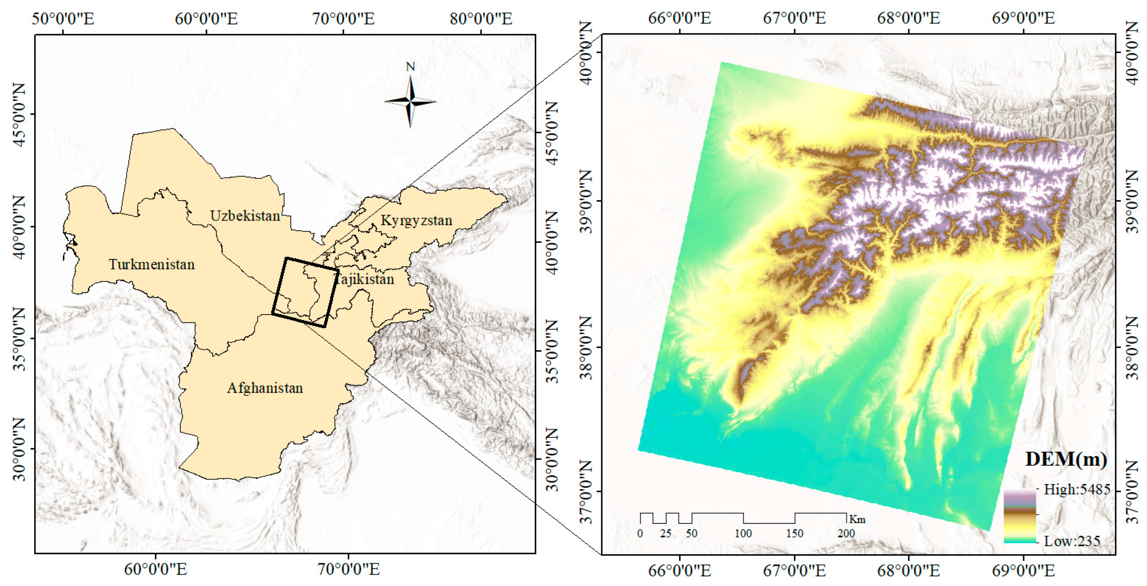
2.1. Study Area

The Surkhan River Basin, located in the southernmost region of Uzbekistan and bordering Tajikistan and Afghanistan, encompasses the Surkhan River and its tributaries within a landscape shaped by complex topographic and hydrological interactions (Figure 1). This region represents a distinct mountain–plain transition zone, ranging from approximately 230 m in the piedmont plains to over 5400 m in the Gissar Range, forming a complete and representative mountain vertical zonation structure within an arid Central Asian inland region. The climate is predominantly arid to semi-arid, characterized by low, highly variable annual precipitation, elevated evapotranspiration rates, and a fragile ecological setting. This topographic complexity, combined with its transitional location between the Central Asian arid zone and high-mountain systems, provides an ideal natural laboratory for studying the dynamics and spatial patterns of mountain vertical zonation under the pressures of climate change and human activities. The Surkhan River Basin has historically served as a hub of human settlement and as a strategic node along the ancient Silk Road, featuring a rich archaeological legacy and notable cultural diversity. Furthermore, the region’s unique climatic conditions and intensive agricultural practices exert significant influences on vegetation distribution and ecological processes along the altitudinal gradient, directly shaping vertical zonation boundaries and transitions. Therefore, selecting the Surkhan River Basin as the study area not only fills a critical research gap in Central Asia but also offers valuable insights into mountain ecosystem responses to environmental changes.

Based on remote sensing imagery and the actual land cover characteristics of the Surkhan River Basin, seven land cover types were identified and classified: cropland, built-up land, water bodies, bare land, grassland, forest, and permanent glaciers/snow cover. Figure 2 illustrates the land cover composition of the Surkhan River Basin. Bare land dominates the region, accounting for 68% of the total area, reflecting the arid environment. Grassland (15%) and cropland (9%) are mainly found in areas with favorable water temperatures, with the remainder accounting for a smaller proportion.

From low to high elevations, the vertical zonation types include the temperate desert zone, mountain grassland zone, alpine cushion vegetation zone, and ice/snow zone, each exhibiting a distinct ecological gradient along an altitudinal continuum (Figure 3).

Table 1. Vertical natural belts and climatic characteristics in the Surkhan River Basin.

Altitudinal Zone (m)	Mean Annual Temperature (°C)	Annual Precipitation (mm)	Vertical Zonation
<1100	15.91	1.10	temperate desert zone
1100–3250	6.27	2.40	mountain grassland zone
3250–3770	−0.48	3.11	alpine cushion vegetation zone
>3770	−1.62	3.01	ice/snow zone

shows the climatic characteristics of the Surkhan River Basin and its corresponding vertical natural zones. The decline in temperature with increasing altitude and the slight increase in precipitation facilitate the transition from desert to grassland, alpine vegetation, and eventually ice/snow environments.

2.2. Data

2.2.1. Landsat Data

Landsat satellite imagery, jointly managed and distributed by the National Aeronautics and Space Administration (NASA) and the United States Geological Survey (USGS), was employed in this study. Data were sourced from Landsat 2 MSS (Multispectral Scanner), Landsat 5 TM (Thematic Mapper), and Landsat 8 OLI (Operational Land Imager), covering the period from 1980 to 2020. All scenes were acquired from the USGS EarthExplorer platform (https://earthexplorer.usgs.gov/ (accessed on 5 June 2024)) and selected based on cloud cover of less than 1% and temporal consistency to ensure comparability across years. To minimize seasonal variability and enhance vegetation signal stability, imagery acquired during the peak growing season (July to September) was used, as this is when vegetation is most active and cloud contamination is typically low.

2.2.2. DEM Data

The digital elevation model (DEM) used in this study was obtained from the Shuttle Radar Topography Mission (SRTM) dataset, provided by the United States Geological Survey (USGS). The SRTM data were acquired during NASA’s Space Shuttle Endeavour mission in February 2000, and provide near-global coverage of Earth’s land surface. The DEM has a spatial resolution of 1 arc seconds (30 m) and has been extensively validated for use in topographic analysis, hydrological modeling, and landform classification.

2.2.3. ERA5 Data

The ERA5 dataset, produced by the European Centre for Medium-Range Weather Forecasts (ECMWF) (https://cds.climate.copernicus.eu/ (accessed on 3 July 2025)) under the Copernicus Climate Change Service, provides high-resolution global reanalysis data with consistent temporal and spatial coverage. ERA5 offers hourly data at a horizontal resolution of 0.1° (~9 km) from 1979 to the present, including a comprehensive suite of atmospheric, land, and oceanic variables. In this study, near-surface air temperature data (2 m temperature) from ERA5 were utilized to analyze long-term climate trends within the Surkhan River Basin, enabling the quantification of regional warming patterns and the assessment of their potential impacts on mountain vertical zonation.

2.2.4. Nighttime Light Data

Nighttime light (NTL) data provide an effective proxy for monitoring human activities, urban expansion, and socioeconomic dynamics at regional and global scales. Li et al. [41] generated a global-scale, integrated, and consistent NTL dataset with a spatial resolution of 30 arc seconds (~1 km) by harmonizing intercalibrated NTL observations from DMSP data and simulated DMSP-like NTL observations from VIIRS data. This study used the data to quantify urbanization trends, farmland expansion, and settlement development, thereby assessing the impact of human activities on mountain vertical zonation and ecological transformation.

2.3. Methods

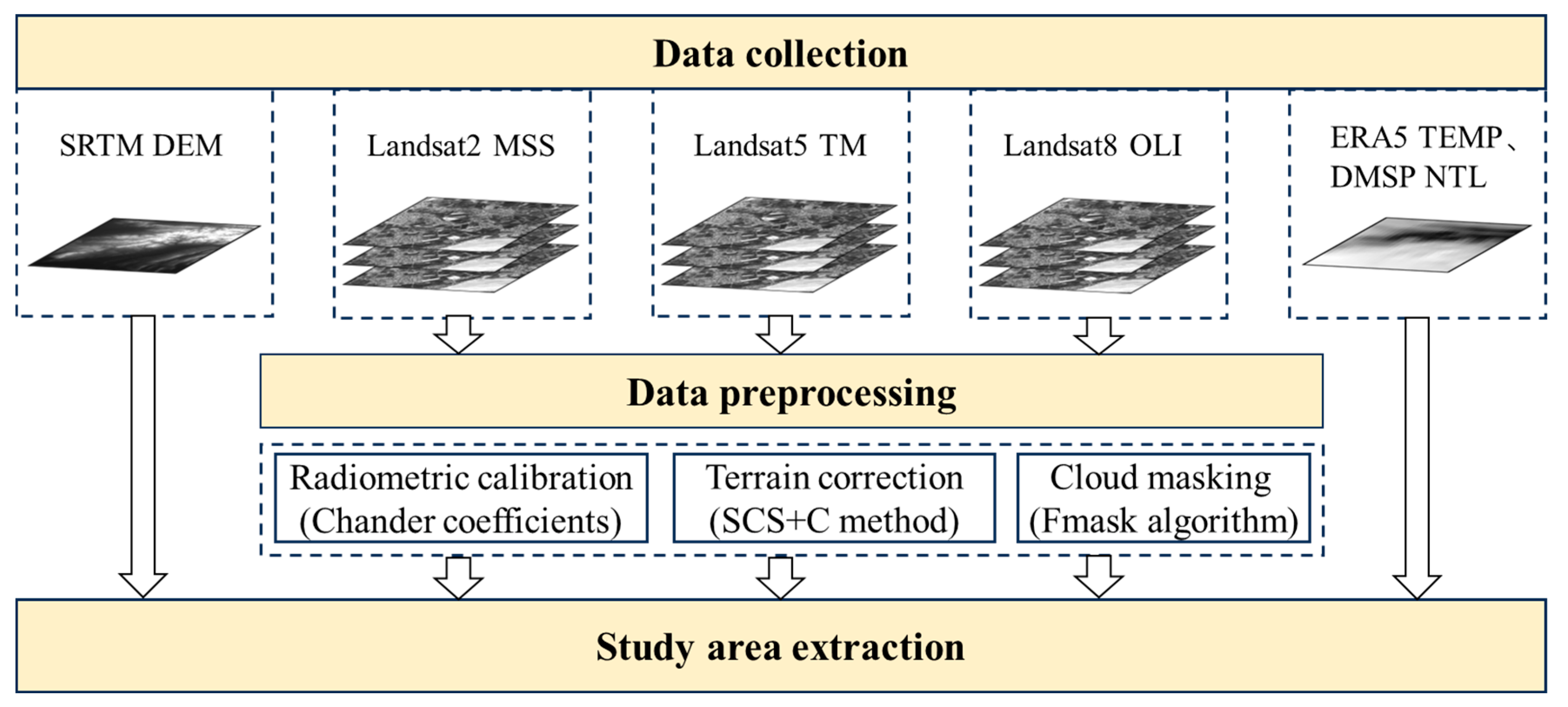
2.3.1. Dataset Preprocessing

The original satellite data used in this study were in the WGS_1984 geographic coordinate system and were uniformly reprojected to the WGS_1984_UTM_Zone_42N coordinate system to ensure spatial consistency. The dataset preprocessing is shown in Figure 4. The processing of Landsat data includes the calibration of radiation, atmospheric correction, terrain correction, and cloud masking.

2.3.2. Vertical Zonation Boundary Extraction

To address the core objective of monitoring and interpreting the spatiotemporal changes in mountain vertical zonation within the Surkhan River Basin, the DEM-NDVI-Land Cover scatterplot analysis is employed to quantitatively delineate the boundaries and structural characteristics of vertical zonation across multiple temporal phases. We spatially overlaid the digital elevation model (DEM), normalized difference vegetation index (NDVI), and land cover classification data. Outliers were removed to enhance data reliability, resulting in a refined dataset. A composite “DEM–NDVI–classification” scatterplot was constructed, where elevation (DEM) was plotted on the horizontal axis and NDVI on the vertical axis. A moving average approach was employed to extract representative NDVI values corresponding to each elevation level. We used a 50% threshold to distinguish the boundaries of vegetation zoning and ecological zoning. In mountainous environments, NDVI or vegetation cover usually has an S-shaped distribution with elevation, and the 50% NDVI threshold corresponds to the mid-range between the peak and trough NDVI values observed along the elevation gradient, which reliably indicates the boundary of a vertical ecotone [31]. Studies on alpine treelines and mountain vegetation zones [42,43,44,45] have successfully used the cumulative threshold to approximate ecological zone boundaries.

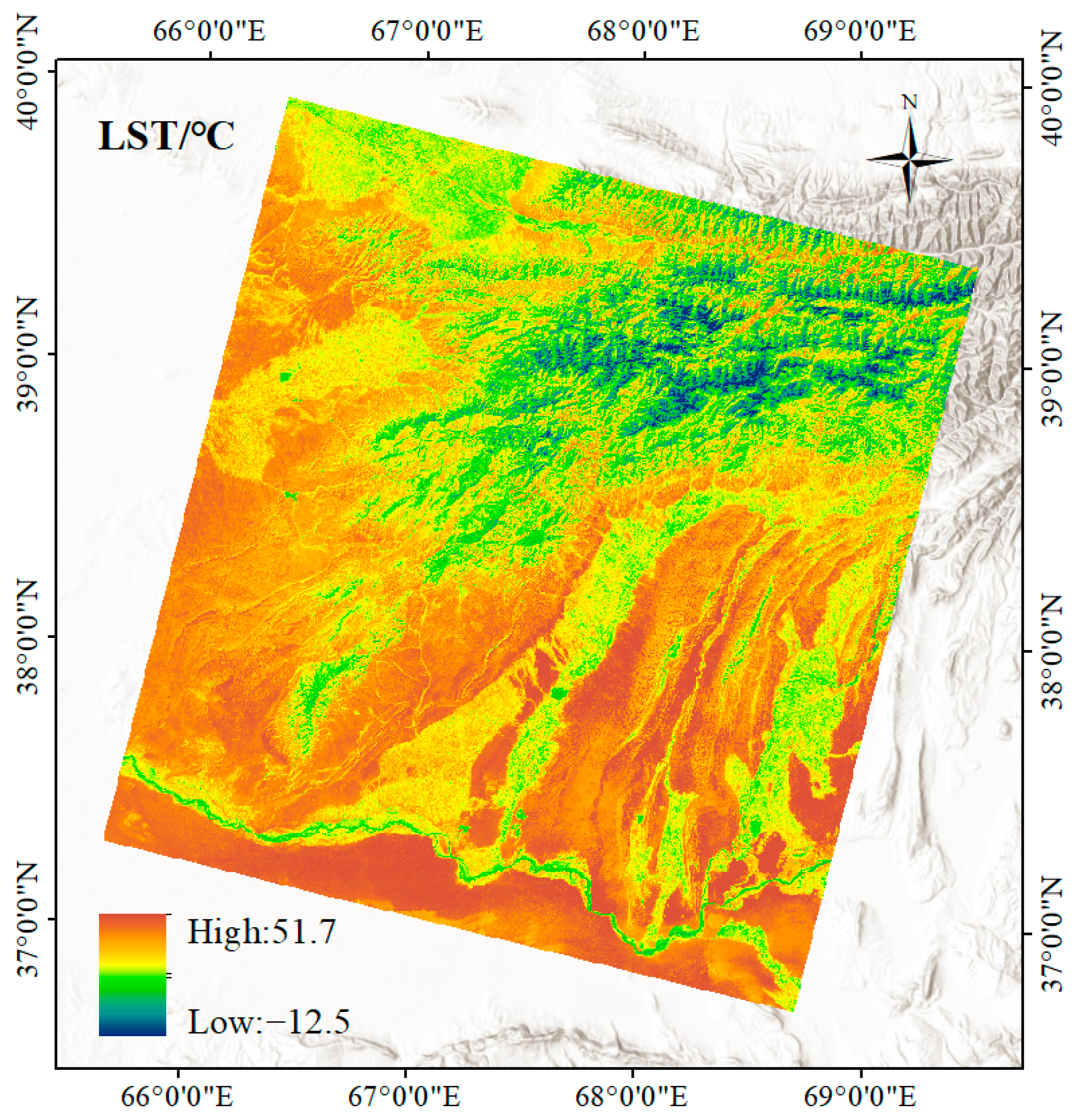
2.3.3. Land Surface Temperature

Land surface temperature (LST) is a critical parameter for understanding land–atmosphere interactions and plays a fundamental role in surface energy balance and ecological processes at both regional and global scales. Among the available algorithms for retrieving LST from Landsat thermal infrared data, the most widely used approaches include the Radiative Transfer Equation (RTE) method [46], the Single-Window (SW) algorithm [47,48], the Universal Single-Channel (USC) algorithm [49,50], the Practical Single-Channel (PSC) algorithm [51], and the Split-Window (SpW) algorithm [52]. Among these, the SW algorithm has been widely recognized for its ability to effectively incorporate surface emissivity and atmospheric radiative effects, while requiring only three key parameters: the atmospheric mean radiative temperature, atmospheric transmittance, and surface emissivity [53,54]. Due to its high accuracy and general applicability, the SW algorithm was adopted in this study for LST retrieval.

The LST retrieval workflow includes the following steps: (1) calculating radiance brightness temperature using Planck’s equation; (2) determining atmospheric mean effective temperature; (3) estimating atmospheric transmittance through MODTRAN simulations; (4) computing surface emissivity for three land cover types: water bodies, urban areas, and natural surfaces; and (5) retrieving surface temperature. All procedures and equations follow well-established methodologies in the literature [47,48,49,50,53,54,55,56,57]. The main process is as follows:

The brightness temperature at the satellite level can be computed by using the following equation.

$$T_B=K_2/\mathrm{l}\mathrm{n}\left(K_1/L_{\lambda }\right)$$

(1)

Here, $K_1$ and $K_2$ are radiation constants. The values of the radiation constants $K_1$ and $K_2$ in the thermal infrared band of Landsat 8 are 774.89 $\mathrm{W}\cdot {\mathrm{m}}^{-2}\cdot \mathrm{s}{\mathrm{r}}^{-1}\cdot \mathsf{\mu }{\mathrm{m}}^{-1}$ and 1321.08 $\mathrm{K}$.

The atmospheric mean temperature is mainly affected by the local atmospheric state and temperature. This study uses the atmospheric mean temperature estimation equation for the mid-latitude region in summer:

$$T_a=16.0110+0.9262T_0$$

(2)

Here, $T_0$ is the temperature at the time of satellite transit, in units of $\mathrm{K}$. Historical temperature data can be found at the relevant website (www.weatherspark.com).

The main factor affecting the calculation of atmospheric transmittance is the atmospheric water vapor content. The water vapor content is determined by the following formula:

$$w=0.0981\times \left[10\times 0.6108\times \mathrm{e}\mathrm{x}\mathrm{p}\left({\displaystyle \frac{17.27\times \left(T_0-273.15\right)}{237.3+\left(T_0-273.15\right)}}\times R(H)\right)\right]+0.1697$$

(3)

Here, $w$ is the total water vapor content of the atmospheric column $(\mathrm{g}\cdot \mathrm{c}{\mathrm{m}}^{-2})$; $R\left(H\right)$ is the ground air humidity $(\%)$. The information of these parameters was provided by the historical weather query website (www.weatherspark.com).

$$\tau =1.0163-0.1330w$$

(4)

Here, $\tau$ is the total atmospheric transmittance.

The types of remote sensing image objects are divided into three types: water body, town, and natural surface. The calculation formulas for the surface emissivity parameters of the water body, town, and natural surface are

$$\begin{array}{c}{\epsilon }_1=0.995\\ {\epsilon }_2=0.9589+0.086P_v-0.0671P_v^2\\ {\epsilon }_3=0.9625+0.0614P_v-0.0461P_v^2\end{array}$$

(5)

where ${\epsilon }_1$, ${\epsilon }_2$, and ${\epsilon }_3$ are the water body emissivity, urban emissivity, and natural surface emissivity, respectively; $P_v$ is the vegetation coverage.

The LST is retrieved from the Landsat 8 data as follows.

$$T_s=\left[a\left(1-C-D\right)+\left(b\left(1-C-D\right)+C+D\right)T_b-D{T}_a\right]/C$$

(6)

$$C=\epsilon \cdot \tau$$

(7)

$$D=(1-\tau )\cdot \left[1+(1-\epsilon )\tau \right]$$

(8)

Here, $T_s$ is the surface temperature; $a$ and $b$ are Planck correlation coefficients, $a=-67.35535,b=0.458608$, respectively; $T_b$ is the brightness temperature of the thermal infrared band; $T_a$ is the average atmospheric temperature; $\epsilon$ is ground emissivity; and $\tau$ is atmospheric transmittance.

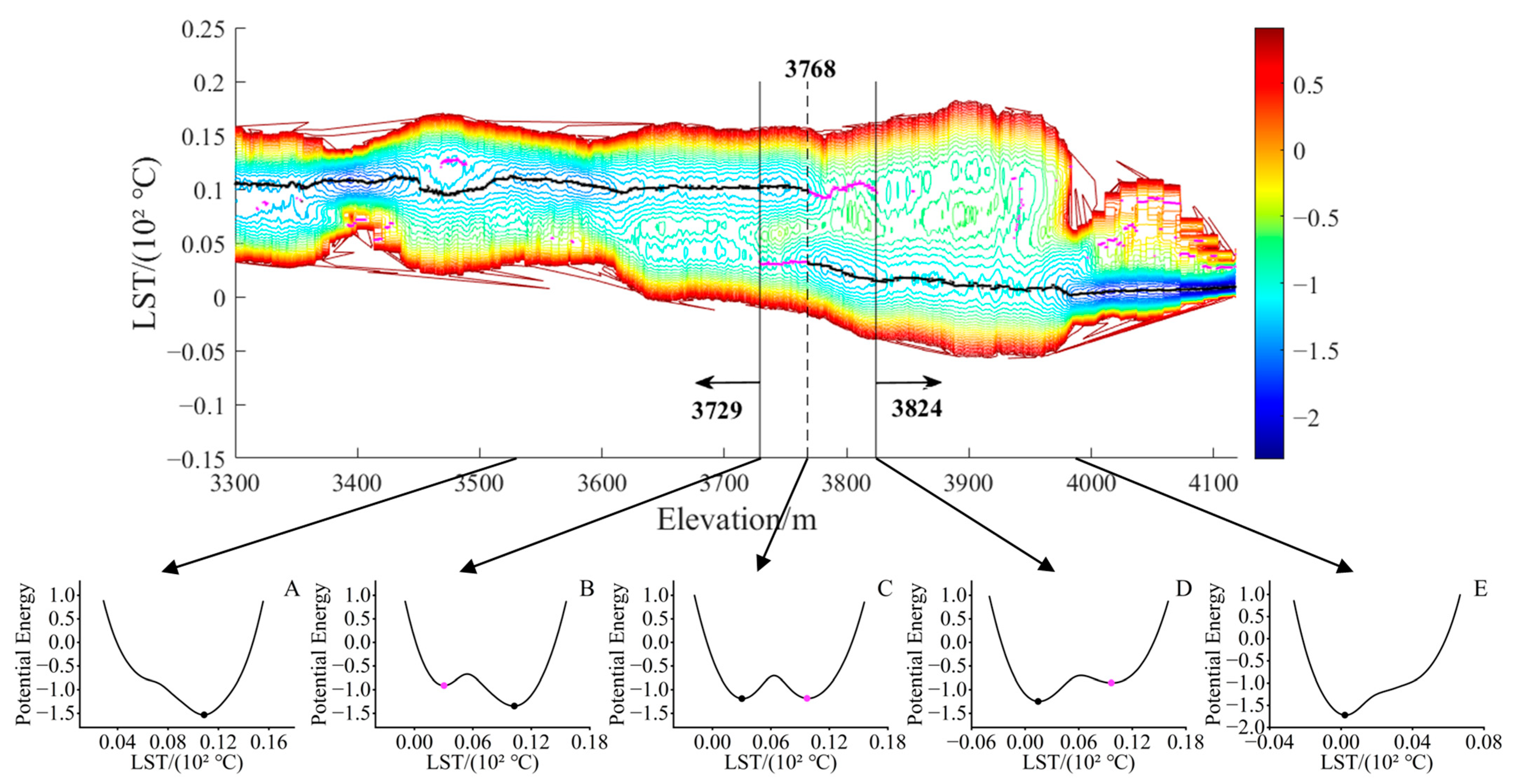
2.3.4. Potential Energy Analysis

To further quantify ecological transition zones and refine altitudinal boundary extraction, potential energy analysis based on LST and DEM is conducted. To further quantify ecological transition zones and refine altitudinal boundary extraction, potential energy analysis based on LST and DEM is conducted. This method captures the bistable states and potential energy differentials within vertical ecotones, providing insight into the dynamic processes driving vertical zonation changes under climate and anthropogenic influences.

In the context of dynamical systems, potential energy analysis provides a systematic framework for evaluating the stability of landscape indicators and their associated driving forces. The potential energy function serves as a quantitative descriptor of a system’s energy state, representing the likelihood of transitions between states or tendencies toward equilibrium. Local minima of the potential energy function denote stable equilibrium states, whereas other regions signify dynamic transitions under the influence of external perturbations, such as climate variability or anthropogenic disturbances. This approach underscores the importance of energy landscape structures in understanding system dynamics and stability [58]. Land surface temperature (LST), as a fundamental component of the Earth’s surface energy budget [59], exhibits strong sensitivity to topographic variation and is widely recognized as an effective indicator of thermal and ecological gradients. In this study, a potential energy analysis model is applied to characterize the spatial distribution of LST-derived potential energy along altitudinal gradients. This enables the identification of ecologically significant transition zones and enhances the interpretation of elevation-driven thermal dynamics.

Potential energy (PE) is typically associated with a system’s state function. For LST analysis, PE is computed using the following formula:

Kernel density estimation is used to estimate the continuous probability density function of the distribution of data points. Given a set of data points $x_1,\dots ,x_n$, $x_i$ is all LST values within that altitude range. Within a window, the distribution of the data points is estimated using a kernel function, $K$:

$$\widehat{f}(x)={\displaystyle \frac{1}{nh}}\sum _{i=1}^{n}K({\displaystyle \frac{x-x_i}{h}})$$

(9)

Here, $\widehat{f}(x)$ is the value of the estimated probability density function at position $x$, $n$ is the number of samples, $x_i$ is the i-th observation in the sample data, and $h$ is the bandwidth parameter. The Silverman rule of thumb is applied to calculate the bandwidth $h$ as follows:

$$h=0.9\times \mathrm{m}\mathrm{i}\mathrm{n}(\sigma ,{\displaystyle \frac{IQR}{1.34}})\times n^{-1/5}$$

(10)

Here, $\sigma$ is the sample standard deviation, $IQR$ is the interquartile range (75–25%), $n$ is the sample size, and after calculation $h=1.06s/n^{1/5}$. After calculating the kernel density estimate, the potential energy value $PE$ can be computed using the following formula:

$$PE(x)=-{\displaystyle \frac{1}{2}}\mathrm{l}\mathrm{o}\mathrm{g}(\widehat{f}(x))$$

(11)

Here, $\widehat{f}(x)$ is the estimated probability density value, while the potential energy value $PE(x)$ reflects the density of the data points. Lower potential energy values typically indicate transitional or changing regions in the area.

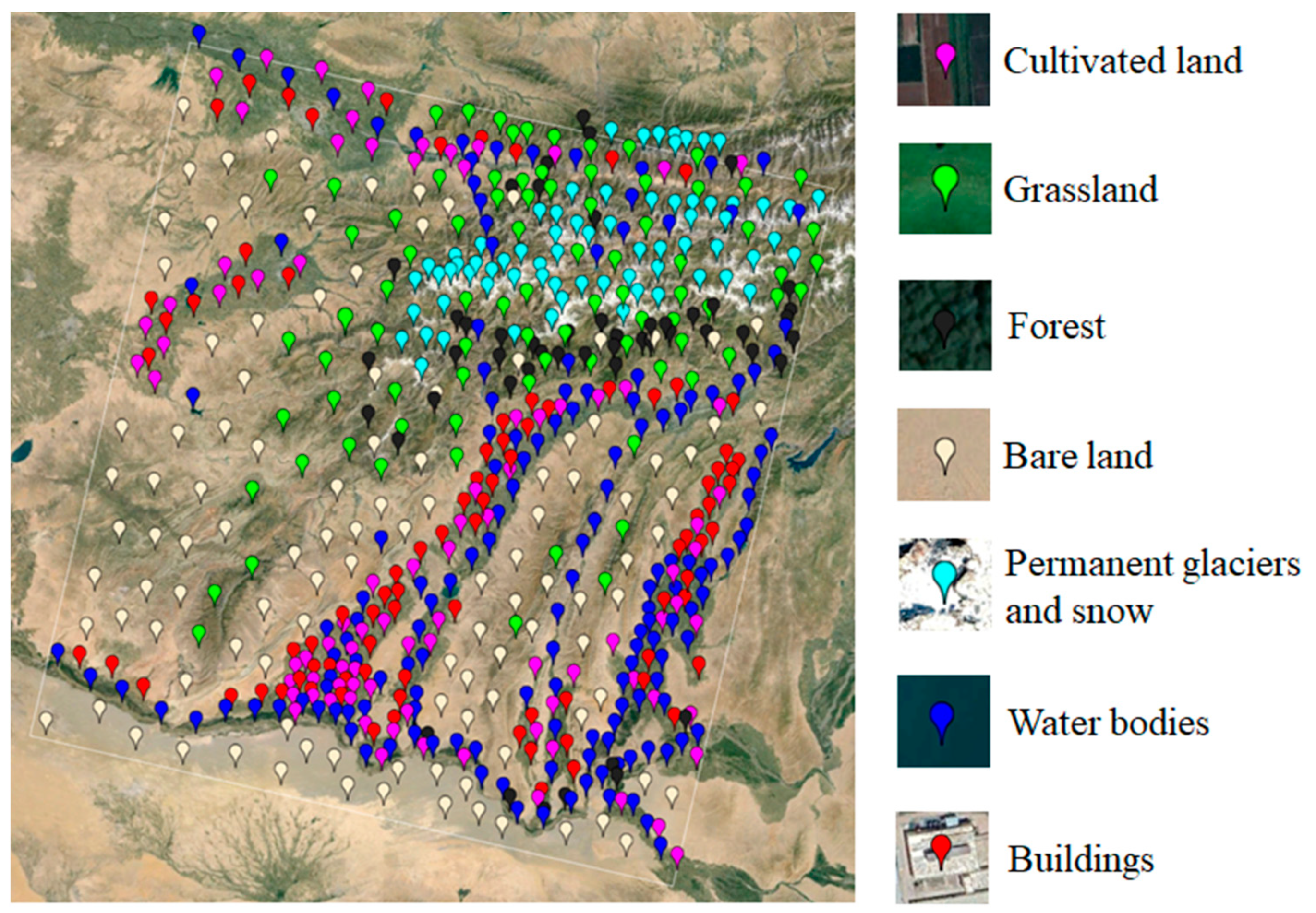
2.3.5. Accuracy Assessment

In order to evaluate the accuracy of land cover classification results in different years, this study used Google Earth high-resolution images for accuracy verification. To ensure the classification accuracy of each land cover type, we evenly selected 100 verification points for each land cover type in our study area, and a total of 700 points were selected for verification (Figure 5). The results revealed that the overall classification accuracy for these periods reached approximately 80%, with Kappa coefficients averaging around 0.76. These metrics confirm that the land cover classification results are sufficiently accurate to support the subsequent spatiotemporal analyses presented in this study.

3. Results

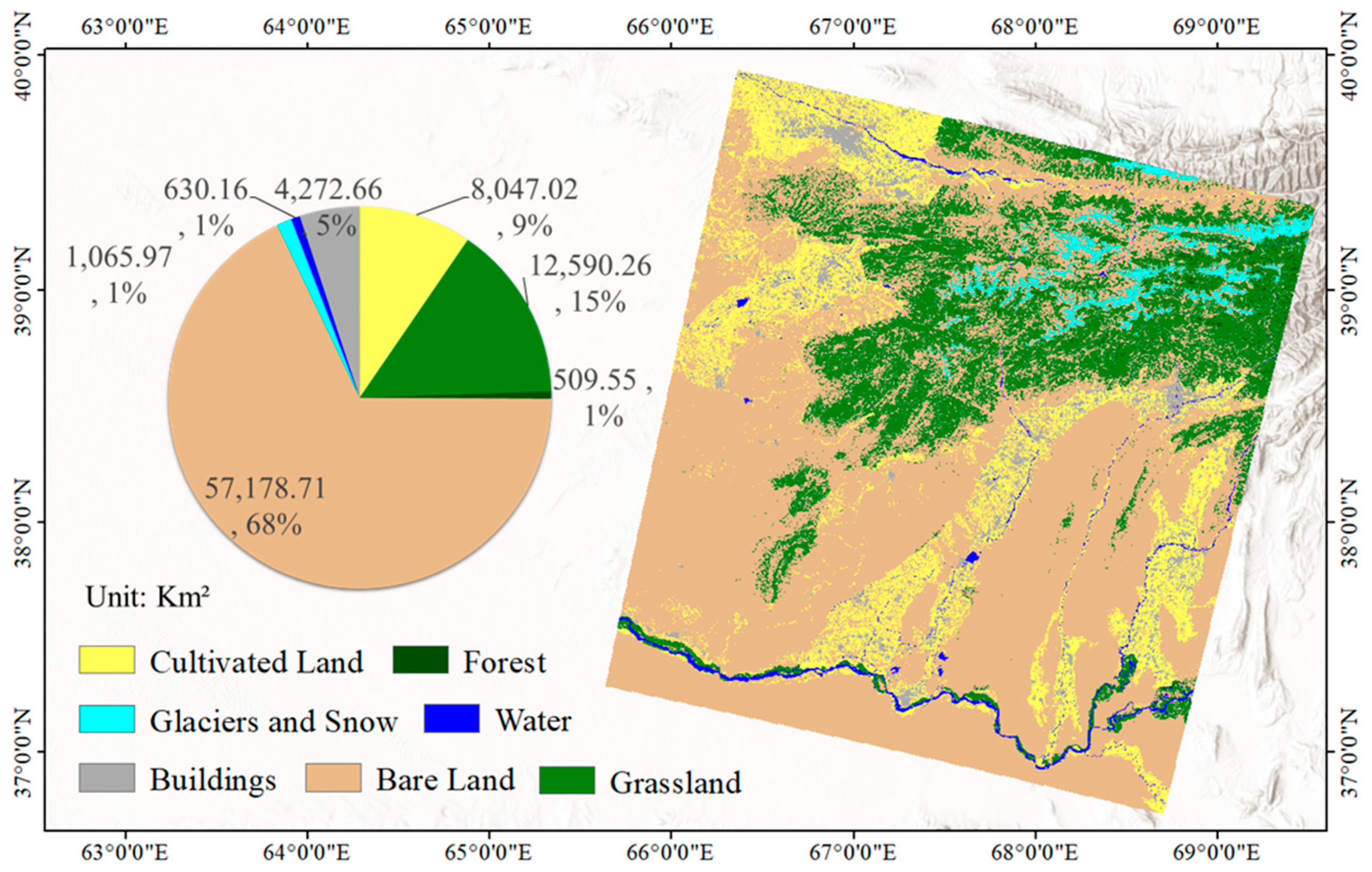
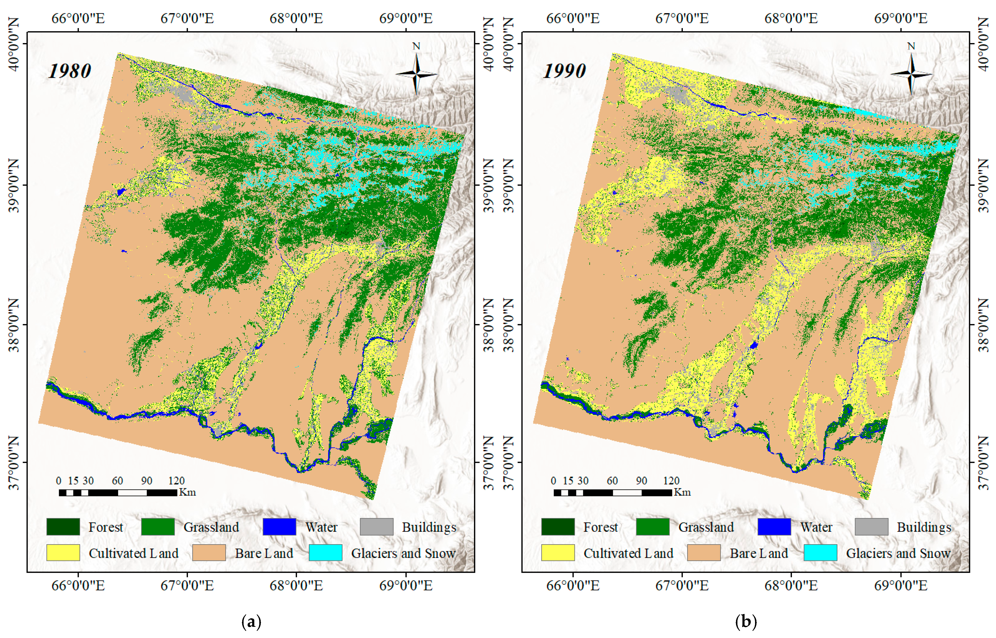
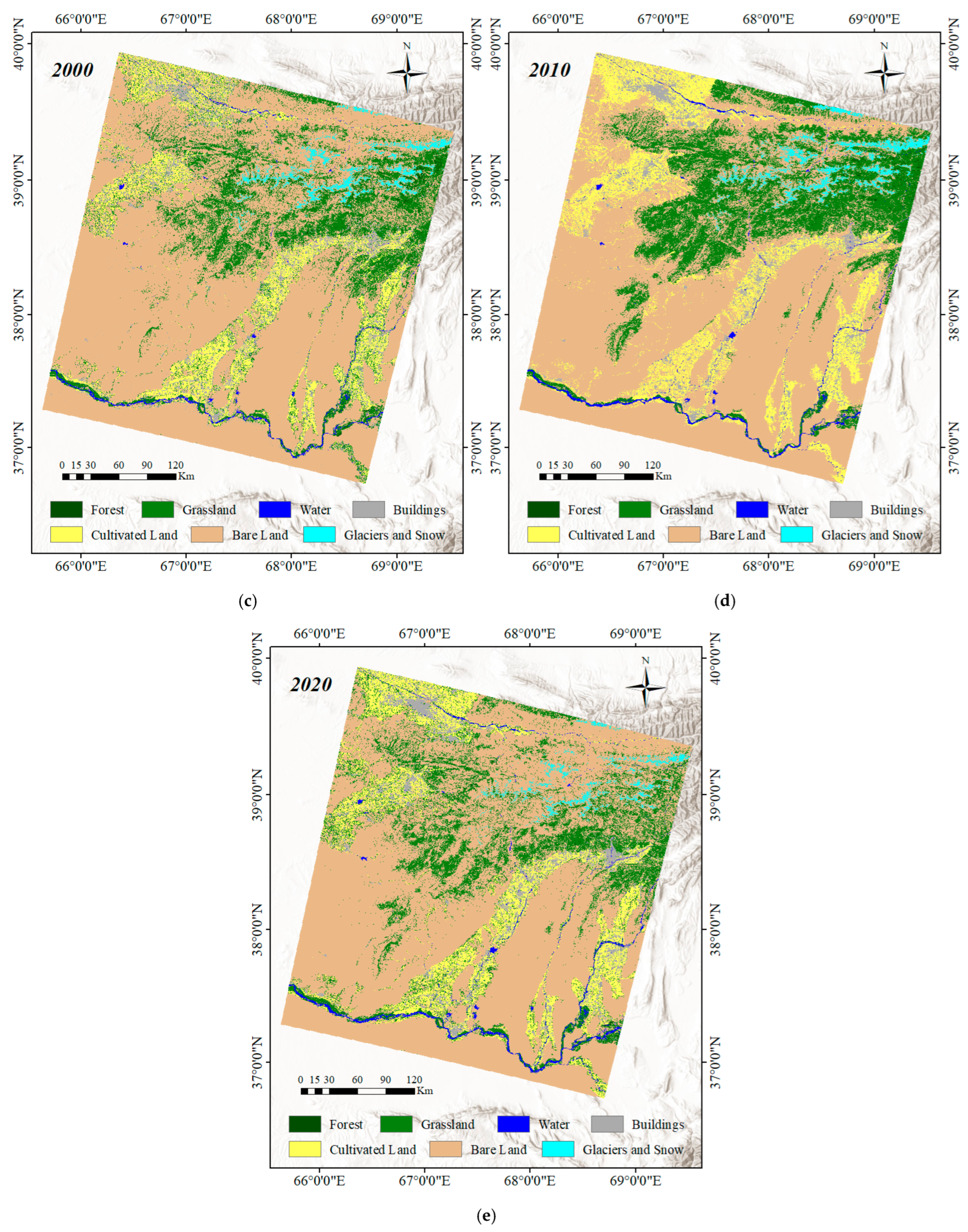
3.1. Land Cover Classification in the Surkhan River Basin

In this study, land cover within the Surkhan River Basin was categorized into seven classes: cultivated land, grassland, forest, bare land, permanent glaciers and snow, water bodies, and buildings. The spatial distribution patterns of these land cover types from 1980 to 2020 are illustrated in Figure 6. The analysis indicates a consistent decline in forest cover over the study period, with notable regional variations wherein forested areas are progressively being replaced by ground cover vegetation. Additionally, the extent of grassland has diminished predominantly at higher altitudes, suggesting ongoing land degradation processes. Cropland expansion was mainly concentrated below 1500 m, increasing from 12.3% (1980) to 28.7% (2020), associated with an upward shift of the steppe boundary (R² = 0.82, p < 0.01). Concurrently, the built-up area has exhibited continuous growth, reflecting a notable progression in urbanization and infrastructural development within the region.

3.2. Mountain Vertical Zonation Results in the Surkhan River Basin

3.2.1. “DEM–NDVI–Land Cover Classification” Scatterplot Analysis

This study utilizes MATLAB (v2020) to generate “DEM–NDVI–Land Cover Classification” scatterplots for the Surkhan River Basin in the years 1980, 1990, 2000, 2010, and 2020 (Figure 7). The analysis reveals distinct altitudinal gradients in land cover and vegetation characteristics. At elevations below 1000 m, bare land predominates, representing the temperate desert zone. This region is characterized by extreme aridity and poor vegetation conditions, with NDVI values typically below 0.1, indicating minimal vegetative cover. Between 1000 and 3200 m, soil moisture gradually increases with altitude, while ambient temperature decreases, creating a more favorable hydrothermal environment for vegetation growth. NDVI values exhibit a steady upward trend across this elevation range, marking a transition from desert landscapes to extensive mountain grasslands, where the NDVI reaches its maximum values. In the 3200–3700 m range, declining temperatures begin to constrain vegetation productivity, particularly for grasses. This results in a shift from grassland to alpine cushion vegetation, characteristic of high-altitude environments. From 3700 to 5400 m, severe climatic constraints, including persistent low temperatures and limited liquid water availability, lead to a predominance of permanent snow and glacier cover. In this zone, NDVI values become negative, further confirming the absence of viable vegetation.

To quantitatively assess temporal changes in the NDVI–elevation relationship, one-way ANOVA was conducted across the four time periods, indicating significant differences between years (F = 7.32, p = 0.002). Analysis revealed a 23% increase in the slope of the NDVI–elevation relationship after 1990 (p < 0.05), indicating that vegetation greening with altitude became more pronounced over time under warming and moistening conditions in the basin.

Overall, NDVI values demonstrate a nonlinear pattern with elevation—increasing initially and then gradually declining—reflecting the compound effects of thermal and moisture gradients on vegetation dynamics. By integrating land cover classification with altitudinal analysis, four major vertical zonation types are delineated: the temperate desert zone, mountain grassland zone, alpine cushion vegetation zone, and snow and ice zone. The scatterplot clearly delineates transition boundaries between these zones, underscoring the strong coupling between vegetation patterns, topography, and ecological conditions in mountainous environments.

3.2.2. Results and Analysis of Mountain Vertical Zonation Extraction

Based on the “DEM–NDVI–Land Cover Classification” scatterplots, vertical zonation dynamics within the Surkhan River Basin between 1980 and 2020 were quantitatively assessed (

Table 2. Vertical band spectrum classification results from 1980 to 2020.

Years	Temperate Desert Zone—Mountain Grassland Zone/(M)	Mountain Grassland Zone—Alpine Cushion Vegetation Zone/(M)	Alpine Cushion Vegetation Zone—Ice/Snow Zone/(M)
1980	1000	3190	3680
1990	1010	3200	3700
2000	1020	3210	3720
2010	1050	3230	3730
2020	1100	3250	3770

). The results indicate a discernible upward shift in key ecological boundaries over the past four decades. Specifically, the transition zone between temperate desert and mountain grassland has migrated upward by approximately 100 m; the lower limit of the alpine cushion vegetation zone has risen by 60 m; and the boundary of the snow/ice zone has shifted upward by 90 m. These altitudinal shifts reflect a broader trend of vertical zonation displacement driven primarily by regional warming. Elevated temperatures have intensified glacier melt during spring and summer months, while reducing the potential for snowpack regeneration in winter, ultimately leading to an upward displacement of the snow line. Simultaneously, warming-induced increases in high-altitude temperatures and meltwater availability have enhanced hydrothermal conditions, promoting the upslope expansion of mountain grasslands. In addition to climate factors, anthropogenic disturbances have also played a significant role. Agricultural encroachment and overgrazing in mid-elevation zones have degraded grassland ecosystems, contributing to the upward migration of the grassland’s lower boundary. Collectively, these findings highlight the combined impacts of climate change and land-use pressures on the spatial reconfiguration of mountain ecosystems in arid and semi-arid environments.

3.3. Critical Transitions in Altitudinal Zonality

Land surface temperature (LST) is a fundamental variable within the Earth’s climate system [59], serving as a key indicator of energy and moisture exchange processes between the land surface and the atmosphere. It directly influences plant phenology and productivity [60], and plays a pivotal role in the assessment of surface energy balance [61], urban heat island effects [62], and global climate change [63]. Compared with NDVI, LST shows more direct sensitivity to the surface energy state, and can better reflect the change in energy state in the ecological transition zone. Although NDVI can also demonstrate bistable characteristics under certain conditions, its values are indirectly influenced by vegetation structure, moisture, and background soil [64]. In contrast, LST can present clearer bimodal or multimodal distributions across elevation gradients, especially in the transition zones where surface energy conditions change dramatically [65]. Therefore, in this study, LST is chosen as the core variable for potential energy analysis to more accurately capture the energy-stabilized structures and bistable phenomena along the elevation gradient, and thus to improve the accuracy of transition zone boundary detection.

As illustrated in Figure 8, the spatial distribution of LST across the Surkhan River Basin exhibits a clear altitudinal gradient, with temperatures decreasing as elevation increases. This inverse relationship corresponds to the well-documented lapse rate phenomenon observed in mountainous environments, underscoring the tight coupling between thermal dynamics and topography in shaping vertical ecosystem structures.

By integrating elevation data with land surface temperature (LST), the potential energy model is employed to invert the potential energy distribution associated with different ecosystem states, with a particular emphasis on the mountain grassland and snow/ice zones—two ecologically sensitive regions within the mountainous environment. These zones exhibit heightened responsiveness to both climatic variability and anthropogenic pressures. The potential energy framework offers a quantitative basis for delineating ecological transition areas and refining the elevation thresholds of altitudinal zones, thereby contributing to a more precise characterization of vertical ecological structures.

3.3.1. Temperate Desert Zone–Mountain Grassland Zone

Figure 9 depicts the elevation-dependent distribution of land surface temperature (LST) and the associated potential energy variations within the transition zone between the temperate desert and mountain grassland zones. The region between the two solid black vertical lines (altitude 1078–1139 m) is where the LST bistable states coexist. The dashed black vertical line (altitude 1110 m) marks the point where the potential energy of the high-LST state starts to exceed that of the low-LST state, indicating a tendency for the system to transition to the low-LST state. Analysis of Figure 9A–E reveals a progression of state coexistence and transitional dynamics across elevation gradients. At lower elevations (Figure 9A), the system is characterized by a single high-LST state, corresponding to low potential energy, indicating a stable and dominant thermal regime. Within the 1078–1139 m elevation range (Figure 9B–D), this region represents the core ecological transition zone. Black data points indicate locations with reduced potential energy, signifying the emergence of bistable conditions—coexisting high- and low-LST states. Among these, the high-LST state is associated with lower potential energy and exhibits stronger system attraction, suggesting dominance. At approximately 1110 m (Figure 9C), which is identified as the boundary between the temperate desert and mountain grassland zones, the energy configuration shifts: high-LST states begin to exhibit increased potential energy and reduced stability, while low-LST states become energetically favorable. At higher elevations (Figure 9E), the system transitions predominantly to a stable low-LST state, reflected by lower potential energy and indicating the establishment of a new dominant thermal regime.

3.3.2. Alpine Cushion Vegetation Zone–Snow/Ice Zone

Figure 10 illustrates the distribution of land surface temperature (LST) along elevation and its relationship with potential energy within the alpine cushion vegetation–snow/ice transition zone. The region between the two solid black vertical lines (altitude 3729–3824 m) is where the LST bistable states coexist. The dashed black vertical line (altitude 3768 m) marks the point where the potential energy of the high-LST state starts to exceed that of the low-LST state, indicating a tendency for the system to transition to the low-LST state. Analysis of Figure 10A–E reveals a similar pattern of coexisting states and key transitions: At lower elevations (Figure 10A), the system exhibits only a high-LST state. The corresponding potential energy value is low, indicating a relatively stable condition. Between elevations of 3729 and 3824 m (Figure 10B–D), this range marks the transition zone between the alpine cushion vegetation and snow/ice zones. Black points indicate areas where LST shows lower potential energy, reflecting the emergence of two coexisting stable states—high and low LST. The high-LST state maintains a lower potential energy and demonstrates stronger attraction than the low-LST state. At 3768 m (Figure 10C), identified as the boundary elevation between the alpine cushion vegetation zone and the snow/ice zone, the system begins to exhibit changes in the potential energy characteristics of the high-LST state. The high-LST state now presents higher potential energy and weaker attraction compared to the low-LST state. At higher elevations (Figure 10E), the system predominantly shifts to a low-LST state, with potential energy values indicating a relatively stable condition.

3.3.3. Bistable Coexistence Zone

The bistable coexistence zone refers to the situation where two different ecosystem states (such as desert state and grassland state) can coexist for a long time within the same altitude range under certain environmental conditions (such as precipitation, temperature, and slope microenvironment). The formation of this bistable structure is usually affected by the combined effects of regional climate fluctuations, microtopography, and human activities, and is an important manifestation of the stability and vulnerability of arid ecosystems.

Figure 11a shows the main vertical zoning boundaries of the Surkhan River Basin: the green line (1100 m above sea level) is the boundary between the temperate desert zone and the mountain grassland zone. The turquoise line (3770 m above sea level) is the boundary between the alpine cushion vegetation zone and the ice and snow zone. Figure 11b,c show bistable coexistence areas: The middle green line (1100 m) shows the location of the ecological dividing line. The upper and lower white lines (1078 m, 1139 m) indicate the range of the bistable coexistence zone extracted by potential energy analysis; i.e., the region has a local alternating distribution of desert vegetation and mountain steppe vegetation under microtopography and microclimate conditions.

3.4. Driving Factor Analysis

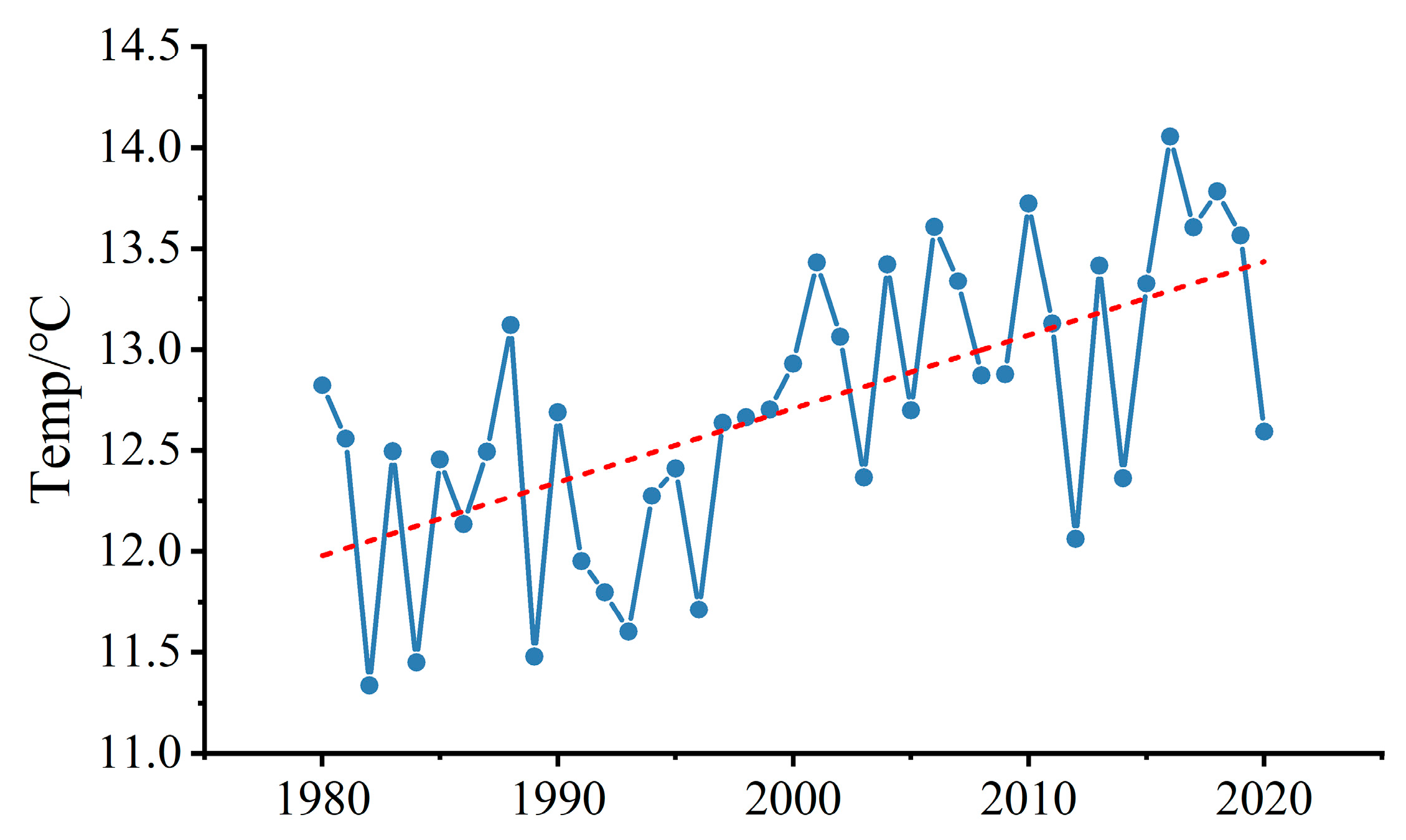
3.4.1. Temperature Change Analysis

To refine the analysis of climate-driven mechanisms, we utilized ERA5 reanalysis data to evaluate the temperature changes in the Surkhan River Basin from 1980 to 2020 (Figure 12). The results show a clear warming trend, with an increase in annual mean temperature from approximately 12.0 °C in the early 1980s to around 13.5 °C in the late 2010s. Our calculated rate of warming (0.34 °C/decade) exceeds the global average rate of warming in mountainous regions (0.25 °C/decade), which accounts for the accelerated retreat of the snow line (2.3 m/year vs. 1.8 m/year in the Tian Shan).

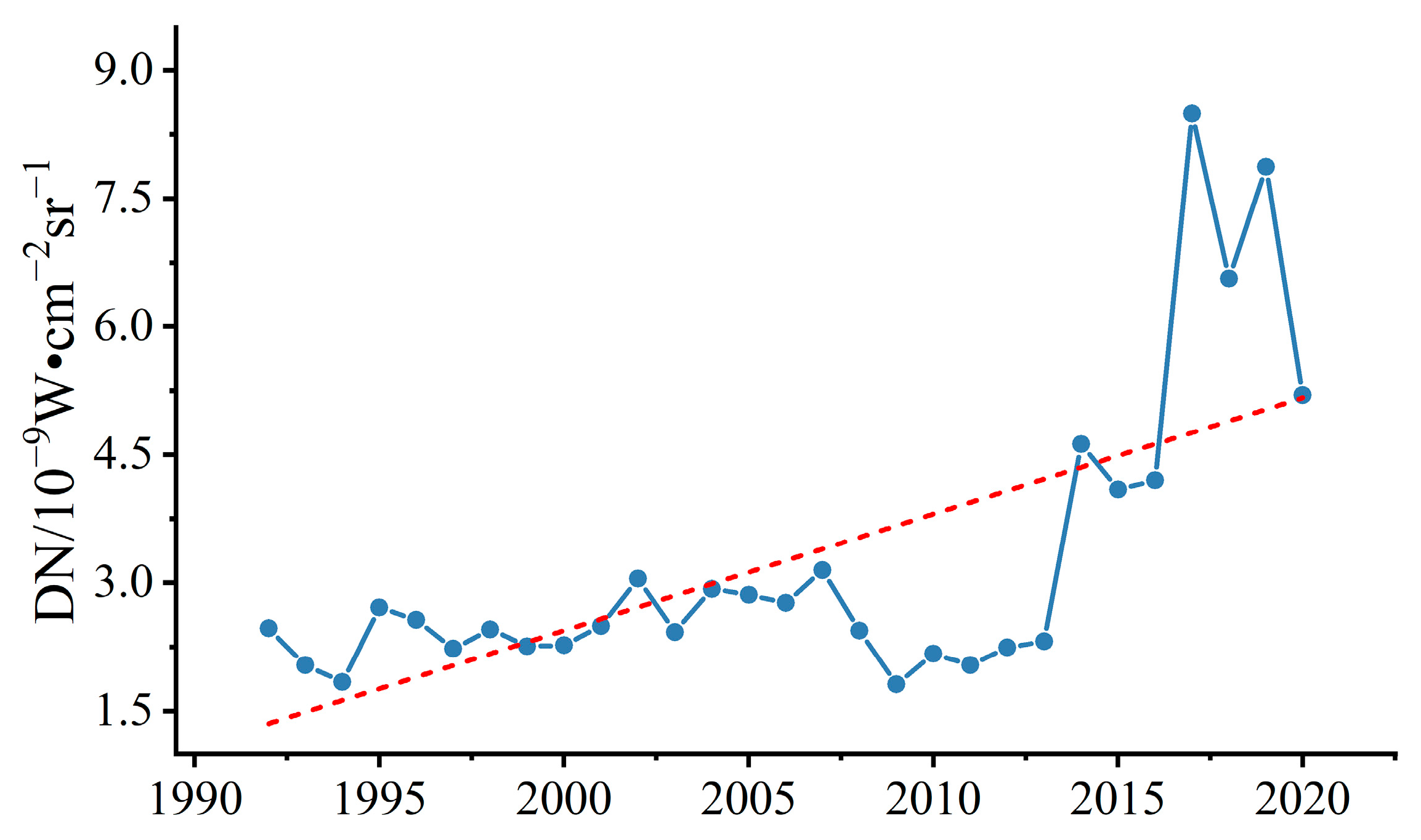
3.4.2. Night Lighting Data Analysis

To quantify anthropogenic impacts on mountain vertical zonation, we utilized nighttime light (NTL) data from DMSP/OLS and VIIRS to assess human activity intensity in the Surkhan River Basin from 1992 to 2020 (Figure 13). The results demonstrate a clear upward trend in nighttime light intensity, with DN values increasing from approximately 2.0 in the early 1990s to over 7.5 after 2015, indicating a 3.8-fold increase over the study period. Enhanced nighttime lighting serves as a proxy for increased infrastructure development and population density, thereby reflecting accelerated anthropogenic disturbances in the region. These changes result in vegetation degradation and fragmentation, which in turn alter the boundaries of ecological transition zones and vertical zonation.

4. Discussion

4.1. Regional Specificity and Methodological Comparison

The mountains of the Central Asian arid zones, such as the Gissar Range in the Surkhan River Basin, exhibit unique vertical zonation characteristics compared to the Himalayas or Alps, primarily due to extreme aridity, high potential evapotranspiration, and strong seasonal snow melt dynamics [66]. Unlike the Himalayas, which exhibit moist adiabatic gradients and a strong monsoonal supply [67], or the Alps, which receive abundant orographic precipitation [68], the Central Asian mountains are characterized by sharp hydrothermal thresholds, resulting in nonlinear and abrupt NDVI transitions along narrow elevation bands. This high sensitivity to interannual and seasonal precipitation variability makes the region particularly responsive to climate variability and human activities, with minor hydrothermal fluctuations triggering significant upward or downward shifts in vegetation boundaries [69,70,71,72].

Methodologically, potential energy analysis provides a robust and physically interpretable approach for refining vertical zonation boundaries, directly capturing bistable states and critical transition points within ecological gradients [33,34]. Compared with MaxEnt [73,74], Random Forest [75,76], and Support Vector Machine (SVM) [77,78], which primarily rely on presence–absence data or produce categorical outputs with limited interpretability regarding underlying energy differentials, potential energy analysis offers a clearer insight into the hydrothermal and energy constraints governing ecological boundaries. This is particularly valuable in arid mountain regions, where microclimatic and topographic variations induce sharp transitions over small elevation intervals that probabilistic or categorical methods may overlook [79,80].

4.2. Leveraging Bistable Transition Zones for Ecological Risk Assessment

According to the extraction results of the mountain grassland zone and the ice/snow zone in 2020, the high consistency between the DEM-NDVI scatterplot and potential energy analysis results—where boundary differences are within 10–32 m—suggests that the scatterplot method is already robust and effective for delineating macro-scale vertical zonation boundaries. The slight numerical differences themselves may hold limited ecological significance at the macro scale, but they are methodologically important in highlighting the distinct capabilities of potential energy analysis. Potential energy analysis provides a more refined characterization of ecological transition regions, not merely by providing a slightly different “accurate” value, but by revealing the range (e.g., 1078–1139 m) and internal bistable instability structure within transition zones. This offers insights into the ecological complexity and spatial heterogeneity of transition zones, which cannot be captured by single-line boundary extractions.

Mountain vertical zonation reflects the integrated responses of regional hydrothermal conditions, vegetation dynamics, and human activities, making it a sensitive indicator of ecosystem changes under climate change and anthropogenic pressures. Using the DEM–NDVI scatterplot, we extracted the vertical zones of the Surkhan River Basin from 1980 to 2020 and observed continued upward shifts in regional boundaries. Specifically, the transition zone between the temperate desert and mountain grassland has migrated at an average rate of 2.5 m/year, while the ice and snow zone, indicative of glacier and snow melt, has shifted upward at an average rate of 2.25 m/year. These trends underscore the strong climatic sensitivity of vertical zonation under the warming and moistening conditions in Central Asia.

To enhance ecological security monitoring and mitigate potential ecological risks, we used potential energy analysis to identify key vertical transition zones in 2020. The transition from temperate desert to mountain grassland was located between 1078 and 1139 m, while the transition from alpine cushion vegetation to ice and snow occurred between 3729 and 3824 m. These elevation bands represent areas of high ecological sensitivity and vulnerability to climate change and anthropogenic disturbances, functioning as tipping points where minor perturbations can lead to abrupt shifts in vegetation states and ecosystem services [81,82]. Incorporating these bistable zones into ecological risk assessment frameworks can improve early warning systems for environmental degradation and guide conservation prioritization and sustainable land-use planning in regions where ecological systems are highly sensitive to external pressures.

4.3. Implications, Limitations, and Future Prospects

Accurate delineation of mountain zonation and transition zones underpins the design of ecological redlines and the monitoring of ecological security in regions under high anthropogenic pressure [83], such as the Surkhan River Basin, which faces intensified agricultural expansion, grazing, and water scarcity under climate change [83]. Integrating findings from potential energy analysis with frameworks from ecological security assessments in highly disturbed regions can enhance risk evaluation and support adaptive management and sustainable land-use planning across the Central Asian arid mountains.

However, this study did not account for the potential “CO₂ fertilization effect” on NDVI, which may affect interpretations of vegetation greening trends. Future studies should integrate FLUXNET data to assess the influence of atmospheric CO₂ enrichment on vegetation dynamics. Additionally, due to methodological differences, we did not directly calculate OA and Kappa values for potential energy analysis, which limits quantitative comparisons with machine learning and MaxEnt methods. Future research should systematically benchmark potential energy analysis against these methods using OA, Kappa, and boundary error distance metrics to enhance the methodological robustness and application value of potential energy analysis in mountain vertical zonation research.

5. Conclusions

Potential energy analysis significantly enhances the precision of ecological transition zone identification in mountainous environments, achieving a 68% improvement in boundary delineation accuracy compared to the DEM–NDVI scatterplot method. This advancement underscores the value of potential energy-based frameworks for capturing the inherent instability and width of transition zones, which is critical for ecological monitoring and landscape gradient analysis.

Analysis of the Surkhan River Basin reveals that the sensitivity of vertical zonation shifts in arid and semi-arid mountain regions is 1.4 times higher than in humid mountain systems under comparable warming rates, highlighting the fragility of Central Asian mountain ecosystems to climate change and anthropogenic pressures. This finding emphasizes the need for region-specific management strategies in arid mountainous regions.

Based on the integration of potential energy analysis, scatterplot boundary extraction, ERA5 warming trends, and nighttime light data indicating intensified human activities, it is recommended to establish an ecological redline at the 1110 m elevation, corresponding to the boundary between the temperate desert zone and the mountain grassland zone. This elevation threshold can serve as a critical reference for ecological conservation, spatial planning, and adaptive management to safeguard transition zones that are vulnerable to compound climate and human-induced stresses.

References

1. Qu, S.; Wang, L.; Lin, A.; Zhu, H.; Yuan, M. What drives the vegetation restoration in Yangtze River basin, China: Climate change or anthropogenic factors? Ecol. Indic. 2018, 90, 438–450. [Google Scholar] [CrossRef]
2. White, A.B.; Kumar, P.; Tcheng, D. A data mining approach for understanding topographic control on climate-induced inter-annual vegetation variability over the United States. Remote Sens. Environ. 2005, 98, 1–20. [Google Scholar] [CrossRef]
3. Li, Q.; Lu, H.; Zhu, L.; Wu, N.; Wang, J.; Lu, X. Pollen-inferred climate changes and vertical shifts of alpine vegetation belts on the northern slope of the Nyainqentanglha Mountains (central Tibetan Plateau) since 8.4 kyr BP. Holocene 2011, 21, 939–950. [Google Scholar] [CrossRef]
4. Biswas, O.; Ghosh, R.; Agrawal, S.; Morthekai, P.; Paruya, D.K.; Mukherjee, B.; Bera, M.; Bera, S. A comprehensive calibrated phytolith based climatic index from the Himalaya and its application in palaeotemperature reconstruction. Sci. Total Environ. 2021, 750, 142280. [Google Scholar] [CrossRef] [PubMed]
5. Wang, H.; Song, Y.; Cheng, Y.; Luo, Y.; Zhang, C.n.; Gao, Y.; Qiu, A.a.; Deng, L.; Liu, H. Mineral magnetism and other characteristics of sediments from a sub-alpine lake (3080 m asl) in central east China and their implications on environmental changes for the last 5770 years. Earth Planet. Sci. Lett. 2016, 452, 44–59. [Google Scholar] [CrossRef]
6. Zhu, C.; Liu, H.; Wang, H.; Feng, S.; Han, Y. Vegetation change at the southern boreal forest margin in Northeast China over the last millennium: The role of permafrost dynamics. Palaeogeogr. Palaeoclimatol. Palaeoecol. 2020, 558, 109959. [Google Scholar] [CrossRef]
7. Wang, W.; He, Z.; Du, J.; Ma, D.; Zhao, P. Altitudinal patterns of species richness and flowering phenology in herbaceous community in Qilian Mountains of China. Int. J. Biometeorol. 2022, 66, 741–751. [Google Scholar] [CrossRef]
8. Dullinger, S.; Dirnböck, T.; Grabherr, G. Modelling climate change-driven treeline shifts: Relative effects of temperature increase, dispersal and invasibility. J. Ecol. 2004, 92, 241–252. [Google Scholar] [CrossRef]
9. Wamucii, C.N.; Van Oel, P.R.; Ligtenberg, A.; Gathenya, J.M.; Teuling, A.J. Land-use and climate change effects on water yield from East African Forested Water Towers. Hydrol. Earth Syst. Sci. Discuss. 2021, 2021, 1389–1406. [Google Scholar] [CrossRef]
10. Anderle, M.; Paniccia, C.; Brambilla, M.; Hilpold, A.; Volani, S.; Tasser, E.; Seeber, J.; Tappeiner, U. The contribution of landscape features, climate and topography in shaping taxonomical and functional diversity of avian communities in a heterogeneous Alpine region. Oecologia 2022, 199, 499–512. [Google Scholar] [CrossRef]
11. Xenarios, S.; Gafurov, A.; Schmidt-Vogt, D.; Sehring, J.; Manandhar, S.; Hergarten, C.; Shigaeva, J.; Foggin, M. Climate change and adaptation of mountain societies in Central Asia: Uncertainties, knowledge gaps, and data constraints. Reg. Environ. Change 2019, 19, 1339–1352. [Google Scholar] [CrossRef]
12. LI, C.-g.; TAN, B.-z. Studies on the methods of mangrove inventory based on RS, GPS and GIS. J. Nat. Resour. 2003, 18, 215–221. [Google Scholar]
13. Zhang, Q.; Zhsng, Y.; Luo, P.; Wang, Q.; Wu, N. Ecological characteristics of cypress population in yang-slope forest line of Baima Mountain. Chin. J. Plant Ecol 2007, 31, 857–864. [Google Scholar]
14. Zhao, F.; Zhang, B.; Zhu, L.; Yao, Y.; Cui, Y.; Liu, J. Spectra structures of altitudinal belts and their significance for determining the boundary between warm temperate and subtropical zones in the Qinling-Daba Mountains. Acta Geogr. Sin 2019, 74, 889. [Google Scholar]
15. Piiroinen, R.; Fassnacht, F.E.; Heiskanen, J.; Maeda, E.; Mack, B.; Pellikka, P. Invasive tree species detection in the Eastern Arc Mountains biodiversity hotspot using one class classification. Remote Sens. Environ. 2018, 218, 119–131. [Google Scholar] [CrossRef]
16. Zhang, Y.; Wu, X.; Zheng, D. Vertical differentiation of land cover in the central Himalayas. J. Geogr. Sci. 2020, 30, 969–987. [Google Scholar] [CrossRef]
17. Chen, W.; Ding, H.; Li, J.; Chen, K.; Wang, H. Alpine treelines as ecological indicators of global climate change: Who has studied? What has been studied? Ecol. Inform. 2022, 70, 101691. [Google Scholar] [CrossRef]
18. Gao, M.; Piao, S.; Chen, A.; Yang, H.; Liu, Q.; Fu, Y.H.; Janssens, I.A. Divergent changes in the elevational gradient of vegetation activities over the last 30 years. Nat. Commun. 2019, 10, 2970. [Google Scholar] [CrossRef]
19. Gómez, C.; White, J.C.; Wulder, M.A. Optical remotely sensed time series data for land cover classification: A review. ISPRS J. Photogramm. Remote Sens. 2016, 116, 55–72. [Google Scholar] [CrossRef]
20. Xie, B.; Jia, X.; Qin, Z.; Shen, J.; Chang, Q. Vegetation dynamics and climate change on the Loess Plateau, China: 1982–2011. Reg. Environ. Change 2016, 16, 1583–1594. [Google Scholar] [CrossRef]
21. Guo, D.; Zhang, H.-y.; Hou, G.-l.; Zhao, J.-j.; Liu, D.-y.; Guo, X.-y. Topographic controls on alpine treeline patterns on Changbai Mountain, China. J. Mt. Sci. 2014, 11, 429–441. [Google Scholar] [CrossRef]
22. Danzeglocke, J.; Oluic, M. Remote sensing of upper timberline elevation in the Alps on different scales. In Proceedings of the 24th EARSeL Symp. New Strategies for European Remote Sensing, Dubrovnik, Croatia, 25–27 May 2005; pp. 25–27. [Google Scholar]
23. Zhang, J.; Yao, Y.; Suonan, D.; Gao, L.; Wang, J.; Zhang, X. Mapping of mountain vegetation in Taibai Mountain based on mountain altitudinal belts with remote sensing. J. Geo-Inf. Sci. 2019, 21, 1284–1294. [Google Scholar]
24. Gao, Y.; Huang, J.; Li, S.; Li, S. Spatial pattern of non-stationarity and scale-dependent relationships between NDVI and climatic factors—A case study in Qinghai-Tibet Plateau, China. Ecol. Indic. 2012, 20, 170–176. [Google Scholar] [CrossRef]
25. Liu, Y.; Li, Z.; Chen, Y.; Li, Y.; Li, H.; Xia, Q.; Kayumba, P.M. Evaluation of consistency among three NDVI products applied to High Mountain Asia in 2000–2015. Remote Sens. Environ. 2022, 269, 112821. [Google Scholar] [CrossRef]
26. Liu, M.; Zhao, R.; Shao, P.; Jiao, J.; Li, L.; Che, Y. Temporal and spatial variation of vegetation coverage and its driving forces in the Loess Plateau from 2001 to 2015. Arid Land Geogr. 2018, 41, 99–108. [Google Scholar]
27. Berner, L.T.; Goetz, S.J. Satellite observations document trends consistent with a boreal forest biome shift. Glob. Change Biol. 2022, 28, 3275–3292. [Google Scholar] [CrossRef]
28. Franke, A.; Feilhauer, H.; Bräuning, A.; Rautio, P.; Braun, M. Remotely sensed estimation of vegetation shifts in the polar and alpine tree-line ecotone in Finnish Lapland during the last three decades. For. Ecol. Manag. 2019, 454, 117668. [Google Scholar] [CrossRef]
29. Bonney, M.T.; Danby, R.K.; Treitz, P.M. Landscape variability of vegetation change across the forest to tundra transition of central Canada. Remote Sens. Environ. 2018, 217, 18–29. [Google Scholar] [CrossRef]
30. Chang, C.; Wang, X.; Yang, R.; Liu, C.; Luo, L.; Zhen, J.; Xiang, B.; Song, J.; Liao, Y. A quantitative characterization method for alpine vegetation zone based on DEM and NDVI. Geogr. Res. 2015, 34, 2113–2123. [Google Scholar]
31. Ji, X.L.; Luo, L.; Wang, X.; Li, L.; Wan, H. Identification and change analysis of mountain altitudinal zone in Tianshan Bogda Natural Heritage Site based on “DEM-NDVI-Land Cover Classification”. J. Geo-Inf. Sci. 2018, 20, 1350–1360. [Google Scholar]
32. Chen, X.; Wang, X.; Li, J.; Kang, D. Species diversity of primary and secondary forests in Wanglang Nature Reserve. Glob. Ecol. Conserv. 2020, 22, e01022. [Google Scholar] [CrossRef]
33. Wan, H.; Wang, X.; Luo, L.; Guo, P.; Zhao, Y.; Wu, K.; Ren, H. Remotely-sensed identification of a transition for the two ecosystem states along the elevation gradient: A case study of Xinjiang Tianshan Bogda world heritage site. Remote Sens. 2019, 11, 2861. [Google Scholar] [CrossRef]
34. Wan, H.; Guo, P.; Luo, L.; Zhao, Y.; Zhao, Y.; Wang, X. Quantitative identification of altitudinal natural zones of mountain vegetation based on ecosystem multi-stable states—A case study of Bogda Mountain in Xinjiang. Natl. Remote Sens. Bull. 2022, 26, 2234–2247. [Google Scholar] [CrossRef]
35. Lioubimtseva, E.; Henebry, G.M. Climate and environmental change in arid Central Asia: Impacts, vulnerability, and adaptations. J. Arid Environ. 2009, 73, 963–977. [Google Scholar] [CrossRef]
36. Malassé, A.D.; Gaillard, C. Relations between climatic changes and prehistoric human migrations during Holocene between Gissar Range, Pamir, Hindu Kush and Kashmir: The archaeological and ecological data. Quat. Int. 2011, 229, 123–131. [Google Scholar] [CrossRef]
37. Worthington, J.R.; Kapp, P.; Minaev, V.; Chapman, J.B.; Mazdab, F.K.; Ducea, M.N.; Oimahmadov, I.; Gadoev, M. Birth, life, and demise of the Andean–syn-collisional Gissar arc: Late Paleozoic tectono-magmatic-metamorphic evolution of the southwestern Tian Shan, Tajikistan. Tectonics 2017, 36, 1861–1912. [Google Scholar] [CrossRef]
38. Konopelko, D.; Seltmann, R.; Mamadjanov, Y.; Romer, R.; Rojas-Agramonte, Y.; Jeffries, T.; Fidaev, D.; Niyozov, A. A geotraverse across two paleo-subduction zones in Tien Shan, Tajikistan. Gondwana Res. 2017, 47, 110–130. [Google Scholar] [CrossRef]
39. Saribaeva, H.S.; Abduraimov, O.; Allamuratov, A. Assessment of the population status of Allium oschaninii O. Fedtsch. in the mountains of Uzbekistan. Ekológia 2022, 41, 147–154. [Google Scholar] [CrossRef]
40. Hagg, W.; Braun, L. The influence of glacier retreat on water yield from high mountain areas: Comparison of Alps and central Asia. Clim. Hydrol. Mt. Areas 2005, 18, 263–275. [Google Scholar]
41. Li, X.; Zhou, Y.; Zhao, M.; Zhao, X. A harmonized global nighttime light dataset 1992–2018. Sci. Data 2020, 7, 168. [Google Scholar] [CrossRef] [PubMed]
42. Prakash Singh, C.; Mohapatra, J.; Pandya, H.A.; Gajmer, B.; Sharma, N.; Shrestha, D.G. Evaluating changes in treeline position and land surface phenology in Sikkim Himalaya. Geocarto Int. 2020, 35, 453–469. [Google Scholar] [CrossRef]
43. Mohapatra, J.; Singh, C.P.; Tripathi, O.P.; Pandya, H.A. Remote sensing of alpine treeline ecotone dynamics and phenology in Arunachal Pradesh Himalaya. Int. J. Remote Sens. 2019, 40, 7986–8009. [Google Scholar] [CrossRef]
44. Danzeglocke, J.; Menz, G. Analysis of upper timberline elevation in the European Alps using MODIS data. In Proceedings of the IGARSS 2004, 2004 IEEE International Geoscience and Remote Sensing Symposium, Anchorage, AK, USA, 20–24 September 2004; pp. 2373–2376. [Google Scholar]
45. Zhao, T.; Bai, H.; Han, H.; Ta, Z.; Li, P.; Wang, P. A Quantitatively Divided Approach for the Vertical Belt of Vegetation Based on NDVI and DEM—An Analysis of Taibai Mountain. Forests 2023, 14, 1981. [Google Scholar] [CrossRef]
46. Chatterjee, R.; Singh, N.; Thapa, S.; Sharma, D.; Kumar, D. Retrieval of land surface temperature (LST) from landsat TM6 and TIRS data by single channel radiative transfer algorithm using satellite and ground-based inputs. Int. J. Appl. Earth Obs. Geoinf. 2017, 58, 264–277. [Google Scholar] [CrossRef]
47. Qin, Z.; Karnieli, A.; Berliner, P. A mono-window algorithm for retrieving land surface temperature from Landsat TM data and its application to the Israel-Egypt border region. Int. J. Remote Sens. 2001, 22, 3719–3746. [Google Scholar] [CrossRef]
48. Bendib, A.; Dridi, H.; Kalla, M.I. Contribution of Landsat 8 data for the estimation of land surface temperature in Batna city, Eastern Algeria. Geocarto Int. 2017, 32, 503–513. [Google Scholar] [CrossRef]
49. Sobrino, J.A.; Jiménez-Muñoz, J.C.; Paolini, L. Land surface temperature retrieval from LANDSAT TM 5. Remote Sens. Environ. 2004, 90, 434–440. [Google Scholar] [CrossRef]
50. Jimenez-Munoz, J.C.; Sobrino, J.A.; Skoković, D.; Mattar, C.; Cristobal, J. Land surface temperature retrieval methods from Landsat-8 thermal infrared sensor data. IEEE Geosci. Remote Sens. Lett. 2014, 11, 1840–1843. [Google Scholar] [CrossRef]
51. Wang, K.; Jiang, Q.-g.; Yu, D.-h.; Yang, Q.-l.; Wang, L.; Han, T.-c.; Xu, X.-y. Detecting daytime and nighttime land surface temperature anomalies using thermal infrared remote sensing in Dandong geothermal prospect. Int. J. Appl. Earth Obs. Geoinf. 2019, 80, 196–205. [Google Scholar] [CrossRef]
52. Li, S.; Jiang, G.-M. Land surface temperature retrieval from Landsat-8 data with the generalized split-window algorithm. IEEE Access 2018, 6, 18149–18162. [Google Scholar] [CrossRef]
53. Wang, F.; Qin, Z.; Song, C.; Tu, L.; Karnieli, A.; Zhao, S. An improved mono-window algorithm for land surface temperature retrieval from Landsat 8 thermal infrared sensor data. Remote Sens. 2015, 7, 4268–4289. [Google Scholar] [CrossRef]
54. Hu, D.; Qiao, K.; Wang, X.; Zhao, L.; Ji, G. Comparison of three single-window algorithms for retrieving land-surface temperature with Landsat 8 TIRS data. Geomat. Inf. Sci. Wuhan Univ. 2017, 42, 869–876. [Google Scholar]
55. Cristóbal, J.; Jiménez-Muñoz, J.; Sobrino, J.; Ninyerola, M.; Pons, X. Improvements in land surface temperature retrieval from the Landsat series thermal band using water vapor and air temperature. J. Geophys. Res. Atmos. 2009, 114, D08103. [Google Scholar] [CrossRef]
56. Jimenez-Munoz, J.C.; Cristobal, J.; Sobrino, J.A.; Sòria, G.; Ninyerola, M.; Pons, X. Revision of the single-channel algorithm for land surface temperature retrieval from Landsat thermal-infrared data. IEEE Trans. Geosci. Remote Sens. 2008, 47, 339–349. [Google Scholar] [CrossRef]
57. Guha, S.; Govil, H.; Diwan, P. Monitoring LST-NDVI Relationship Using Premonsoon Landsat Datasets. Adv. Meteorol. 2020, 2020, 4539684. [Google Scholar] [CrossRef]
58. Berdugo, M.; Kéfi, S.; Soliveres, S.; Maestre, F.T. Plant spatial patterns identify alternative ecosystem multifunctionality states in global drylands. Nat. Ecol. Evol. 2017, 1, 0003. [Google Scholar] [CrossRef]
59. Li, Z.-L.; Tang, B.-H.; Wu, H.; Ren, H.; Yan, G.; Wan, Z.; Trigo, I.F.; Sobrino, J.A. Satellite-derived land surface temperature: Current status and perspectives. Remote Sens. Environ. 2013, 131, 14–37. [Google Scholar] [CrossRef]
60. Peng, S.-S.; Piao, S.; Zeng, Z.; Ciais, P.; Zhou, L.; Li, L.Z.; Myneni, R.B.; Yin, Y.; Zeng, H. Afforestation in China cools local land surface temperature. Proc. Natl. Acad. Sci. USA 2014, 111, 2915–2919. [Google Scholar] [CrossRef]
61. Tajfar, E.; Bateni, S.; Lakshmi, V.; Ek, M. Estimation of surface heat fluxes via variational assimilation of land surface temperature, air temperature and specific humidity into a coupled land surface-atmospheric boundary layer model. J. Hydrol. 2020, 583, 124577. [Google Scholar] [CrossRef]
62. Alexander, C. Normalised difference spectral indices and urban land cover as indicators of land surface temperature (LST). Int. J. Appl. Earth Obs. Geoinf. 2020, 86, 102013. [Google Scholar] [CrossRef]
63. Shen, Y.; Shen, H.; Cheng, Q.; Zhang, L. Generating comparable and fine-scale time series of summer land surface temperature for thermal environment monitoring. IEEE J. Sel. Top. Appl. Earth Obs. Remote Sens. 2020, 14, 2136–2147. [Google Scholar] [CrossRef]
64. Alademomi, A.S.; Okolie, C.J.; Daramola, O.E.; Akinnusi, S.A.; Adediran, E.; Olanrewaju, H.O.; Alabi, A.O.; Salami, T.J.; Odumosu, J. The interrelationship between LST, NDVI, NDBI, and land cover change in a section of Lagos metropolis, Nigeria. Appl. Geomat. 2022, 14, 299–314. [Google Scholar] [CrossRef]
65. Wan, H.; Guo, P.; Luo, L.; Zhao, Y.; Zhao, Y.; Wang, X. Different remote sensing indicators reveal the transitions of two states along elevation gradients within the Xinjiang Tianshan Bogda Natural World Heritage Site. Int. J. Appl. Earth Obs. Geoinf. 2022, 111, 102842. [Google Scholar] [CrossRef]
66. Yu, Y.; Chen, X.; Malik, I.; Wistuba, M.; Cao, Y.; Hou, D.; Ta, Z.; He, J.; Zhang, L.; Yu, R. Spatiotemporal changes in water, land use, and ecosystem services in Central Asia considering climate changes and human activities. J. Arid Land 2021, 13, 881–890. [Google Scholar] [CrossRef]
67. Negi, V.S.; Tiwari, D.C.; Singh, L.; Thakur, S.; Bhatt, I.D. Review and synthesis of climate change studies in the Himalayan region. Environ. Dev. Sustain. 2022, 24, 10471–10502. [Google Scholar] [CrossRef]
68. Gobiet, A.; Kotlarski, S.; Beniston, M.; Heinrich, G.; Rajczak, J.; Stoffel, M. 21st century climate change in the European Alps—A review. Sci. Total Environ. 2014, 493, 1138–1151. [Google Scholar] [CrossRef] [PubMed]
69. Chen, H.; Yang, S.; Picotti, V.; Cheng, X.; Lin, X.; Li, K. The late Cenozoic expansion of the Northeastern Pamir: Insights from the stratigraphic architecture of the Wupoer Piggyback Basin. J. Asian Earth Sci. 2022, 232, 105012. [Google Scholar] [CrossRef]
70. Ding, C.; Huang, W.; Liu, M.; Zhao, S. Change in the elevational pattern of vegetation Greenup date across the Tianshan Mountains in Central Asia during 2001–2020. Ecol. Indic. 2022, 136, 108684. [Google Scholar] [CrossRef]
71. Ding, Q.; Wang, L.; Fu, M. Spatial characteristics and trade-offs of ecosystem services in arid central Asia. Ecol. Indic. 2024, 161, 111935. [Google Scholar] [CrossRef]
72. Liu, W.; Zhang, B.; Wei, Z.; Wang, Y.; Tong, L.; Guo, J.; Han, X.; Han, C. Heterogeneity analysis of main driving factors affecting potential evapotranspiration changes across different climate regions. Sci. Total Environ. 2024, 912, 168991. [Google Scholar] [CrossRef]
73. Elith, J.; Phillips, S.J.; Hastie, T.; Dudík, M.; Chee, Y.E.; Yates, C.J. A statistical explanation of MaxEnt for ecologists. Divers. Distrib. 2011, 17, 43–57. [Google Scholar] [CrossRef]
74. Zhao, Y.; Deng, X.; Xiang, W.; Chen, L.; Ouyang, S. Predicting potential suitable habitats of Chinese fir under current and future climatic scenarios based on Maxent model. Ecol. Inform. 2021, 64, 101393. [Google Scholar] [CrossRef]
75. Sun, Z.; Wang, G.; Li, P.; Wang, H.; Zhang, M.; Liang, X. An improved random forest based on the classification accuracy and correlation measurement of decision trees. Expert Syst. Appl. 2024, 237, 121549. [Google Scholar] [CrossRef]
76. Zhao, Y.; Zhu, W.; Wei, P.; Fang, P.; Zhang, X.; Yan, N.; Liu, W.; Zhao, H.; Wu, Q. Classification of Zambian grasslands using random forest feature importance selection during the optimal phenological period. Ecol. Indic. 2022, 135, 108529. [Google Scholar] [CrossRef]
77. Guo, Z.; Liu, H.; Zheng, Z.; Chen, X.; Liang, Y. Accurate extraction of mountain grassland from remote sensing image using a capsule network. IEEE Geosci. Remote Sens. Lett. 2020, 18, 964–968. [Google Scholar] [CrossRef]
78. Cui, L.; Wang, L.; Su, J.; Song, Z.; Li, X. Classification and identification of degraded alpine m eadows based on machine learning techniques. In Proceedings of the 2023 4th International Conference on Computer Vision, Image and Deep Learning (CVIDL), Zhuhai, China, 12–14 May 2023; pp. 263–267. [Google Scholar]
79. Liao, C.-C.; Chang, C.-R.; Yi-Huey, C. Advantage and Disadvantage of Global and Local Climate Datasets on Modeling Species Distribution at Continental and Landscape Scales. Res. Sq. 2021. [Google Scholar] [CrossRef]
80. Hassija, V.; Chamola, V.; Mahapatra, A.; Singal, A.; Goel, D.; Huang, K.; Scardapane, S.; Spinelli, I.; Mahmud, M.; Hussain, A. Interpreting black-box models: A review on explainable artificial intelligence. Cogn. Comput. 2024, 16, 45–74. [Google Scholar] [CrossRef]
81. Wang, Y.-S.; Gu, J.-D. Ecological responses, adaptation and mechanisms of mangrove wetland ecosystem to global climate change and anthropogenic activities. Int. Biodeterior. Biodegrad. 2021, 162, 105248. [Google Scholar] [CrossRef]
82. Shi, S.; Yu, J.; Wang, F.; Wang, P.; Zhang, Y.; Jin, K. Quantitative contributions of climate change and human activities to vegetation changes over multiple time scales on the Loess Plateau. Sci. Total Environ. 2021, 755, 142419. [Google Scholar] [CrossRef]
83. Moradzadeh, V.; Hazbavi, Z.; Esmali Ouri, A.; Mostafazadeh, R.; Rodrigo-Comino, J.; Zareie, S.; Fernández-Raga, M. A multifunctional conceptual framework for ecological disturbance assessment. Earth Syst. Environ. 2025, 9, 51–69. [Google Scholar] [CrossRef]
Figure 1. Study area extent and geographical location.
Remotesensing 17 02612 g001
Figure 2. Spatial distribution and area share of land cover in the Surkhan River Basin.
Remotesensing 17 02612 g002
Figure 3. Mountain profile of the Surkhan River Basin.
Remotesensing 17 02612 g003
Figure 4. Dataset preprocessing flow chart.
Remotesensing 17 02612 g004
Figure 5. Google Earth verification points.
Remotesensing 17 02612 g005
Figure 6. Land cover classification results in the Surkhan River Basin: (a) 1980, (b) 1990, (c) 2000, (d) 2010, (e) 2020.
Remotesensing 17 02612 g006aRemotesensing 17 02612 g006b
Figure 7. “DEM-NDVI-Land Cover Classification” scatterplot in the Surkhan River Basin: (a) 1980, (b) 1990, (c) 2000, (d) 2010, (e) 2020.
Remotesensing 17 02612 g007
Figure 8. LST distribution map in the Surkhan River Basin.
Remotesensing 17 02612 g008
Figure 9. Variation characteristics of the potential energy value of LST in the temperate desert–mountain grassland zone with altitude gradient: The black and purple-red dots represent local minima of the potential energy. The contour lines represent the spatial distribution of the estimated potential energy values. Panels (AE) illustrate the detailed process of the system transitioning from the high-LST state to the low-LST state with increasing altitude.
Remotesensing 17 02612 g009
Figure 10. Variation characteristics of the potential energy value of LST in the alpine cushion vegetation–snow and ice zone with altitude gradient: The black and purple-red dots represent local minima of the potential energy. The contour lines represent the spatial distribution of the estimated potential energy values. Panels (AE) illustrate the detailed process of the system transitioning from the high-LST state to the low-LST state with increasing altitude.
Remotesensing 17 02612 g010
Figure 11. Schematic diagram of the bistable coexistence zone. (a) Transition elevation range and boundary elevation determined in this study (full view). (b,c) Google earth verifies the identified results.
Remotesensing 17 02612 g011
Figure 12. Temperature change trend chart of Surkhan River Basin from 1980 to 2020.
Remotesensing 17 02612 g012
Figure 13. Trend chart of nighttime lighting changes in the Surhan River Basin from 1992 to 2020.
Remotesensing 17 02612 g013