Martian Skylight Identification Based on the Deep Learning Model

Abstract

As a type of distinctive pit on Mars, skylights are entrances to subsurface lava caves. They are very important for studying volcanic activity and potential preserved water ice, and are also considered as potential sites for human extraterrestrial bases in the future. Most skylights are manually identified, which has low efficiency and is highly subjective. Although deep learning methods have recently been used to identify skylights, they face challenges of few effective samples and low identification accuracy. In this article, 151 positive samples and 920 negative samples based on the MRO-HiRISE image data was used to create an initial skylight dataset, which contained few positive samples. To augment the initial dataset, StyleGAN2-ADA was selected to synthesize some positive samples and generated an augmented dataset with 896 samples. On the basis of the augmented skylight dataset, we proposed YOLOv9-Skylight for skylight identification by incorporating Inner-EIoU loss and DySample to enhance localization accuracy and feature extracting ability. Compared with YOLOv9, the P, R, and the F1 of YOLOv9-Skylight were improved by about 9.1%, 2.8%, and 5.6%, respectively. Compared with other mainstream models such as YOLOv5, YOLOv10, Faster R-CNN, Mask R-CNN, and DETR, YOLOv9-Skylight achieved the highest accuracy (F1 = 92.5%), which shows a strong performance in skylight identification.

1. Introduction

In the 1970s, planetary geologists used remote sensing data to discover some distinct pits on the flank of Olympus Mons on Mars [1,2]. These pits were circular, collapsed, and characterized by overhanging or vertical walls. Cushing et al. [3] defined these pits as “skylights”. Skylights are usually considered to be entrances to subsurface lava caves, which originated from collapsed lava tubes formed by volcanic activity [4]. Therefore, skylights are important for studying volcanic activity and the evolution of Mars [5]. Moreover, some scientists supposed that caves below skylights may provide some resources, including volatiles and potentially even water ice [6,7]. Due to the stable internal environment, skylights are even supposed to protect against strong radiation, temperature fluctuations, and meteorite impacts [8]. Therefore, skylights are considered as promising potential sites for human habitation in the future and astrobiology investigations, making their identification essential for long-term mission planning and development of advanced exploration technologies [9]. As a distinct type of landform, there are also some skylights on the Earth, which are primarily formed by the collapse of lava tubes or karst processes (e.g., the development of karst landforms) [7,10]. Investigating those skylights may provide valuable insights into the origin and characteristics of skylights on Mars.

With the development of high-resolution remote sensing techniques, more and more high-resolution image data has been acquired to identify skylights. Since 2010, some experts have manually identified Martian skylights. Cushing [11] manually identified 1062 skylights in the volcanic regions such as Alba Mons, the Tharsis region, and the Elysium region with MO-THEMIS (Mars Odyssey Thermal Emission Imaging System), MRO-CTX (Mars Reconnaissance Orbiter Context Camera), and MRO-HiRISE (Mars Reconnaissance Orbiter High Resolution Imaging Science Experiment) image data. However, most skylights identified by Cushing using MRO-CTX images were misidentified [11]. Sharma and Srivastava [12] manually identified 26 new skylights on the flanks of the Elysium volcano, with MO-THEMIS, MRO-CTX, and MRO-HiRISE image data. On the north of the Arsia volcano, Tettamanti [4] used MRO-HiRISE and MRO-CTX image data to identify 193 skylights manually, which were used to detect 48 potential lava tubes. Manual identification is an important and direct method to identify skylights, but it spends much time with low efficiency compared with automatic methods. When processing large amounts of data, it will spend a lot of time and labor, which limits its flexibility in applications. Additionally, manual identification is a technique which relies on human experience and knowledge to identify skylights by analyzing the color and morphological features. Due to individual differences, different interpreters may obtain different identified results with strong subjectivity. In order to improve the accuracy, interpreters are required to be trained with sufficient experience. Although manual identification is inefficient and heavily influenced by subjectivity, its intuitiveness and flexibility still hold significant importance. Even in complex backgrounds, it can still achieve a relatively high accuracy. So, manual identification is commonly used to label samples when creating datasets.

In recent years, deep learning has demonstrated significant potential in the field of computer vision, becoming increasingly prevalent in geological structure identification with remote sensing image data [13,14]. Up to now, Nodjoumi et al. [15] have been the only researchers to utilize deep learning methods to identify Martian skylights. They used YOLOv5 to identify negative landforms (including skylights) in the Tharsis region with MRO-CTX and MRO-HiRISE image data. However, as an object detection model, YOLOv5 only provides general localization of negative landforms. To achieve more precise localization and definition of the shapes of these negative landforms, Nodjoumi et al. [16] further employed Mask R-CNN, an instance segmentation model, for the identification of negative landforms. Due to insufficient samples, they built an initial dataset (total: 486·samples, including 125 skylights, 95 bowl-shaped pits, 42 coalescent pits, 133 shallow pits, and 91 craters) and augmented the initial dataset to 2375 samples by downscaling and adding noise firstly. And then, Mask R-CNN·was trained and tested on the augmented dataset, but the identification accuracy is very low (26.7%). During the above process of dataset augmenting, the downscaling compressed the morphological features by reducing image resolution, which may lead to the loss of critical details, and noise addition obscured the important skylight’s characteristics and even introduced misleading information. Additionally, downscaling and noise addition only changed the pixel distribution of the images and failed to produce new semantic content. So, the augmented dataset was unrepresentative and low-quality, which even affected the accuracy of the skylight identification model. Although downscaling and noise addition for data augmentation have not achieved ideal results in skylight identification, data augmentation is still an effective way to solve the problem of few-sample identification tasks with suitable methods [17].

In this article, a modified skylight identification model was proposed, based on an augmented dataset using high-resolution image data. To address the issue of insufficient skylight samples, an initial skylight dataset was created with the MRO-HiRISE image da-ta and augmented using generative models. Based on the YOLOv9, the loss function and upsampling method were modified to enhance the localization accuracy and feature extracting capability. And then, a new skylight identification model—YOLOv9-Skylight—came into being. Finally, some other mainstream object detection models, trained by the same augmented dataset, were used to evaluate the performance of YOLOv9-Skylight.

2. Experimental Areas and Data Processing

As described in the introduction, the augmented dataset [16] is the only available one to train identification models at present. However, due to lack of representativeness and the low quality of the augmented dataset, it is difficult to effectively train identification models. Another way to create a new dataset is based on the existing identified skylights. Though there are some identified skylights, the accuracy is very poor. So, the only way to create the dataset is to identify skylights manually in suitable experiment areas and with appropriate data.

2.1. Experimental Area Selection

In this study, the experimental areas should cover as many skylights as possible. In Figure 1, the identified skylights are mainly distributed in the Tharsis region and the Elysium region (see the green circles in Figure 1) [4,11,12]. Some geophysical surveys [18,19] revealed that there had been high influxes of lava flow in those areas, which explained why there are so many skylights. Except for the above areas, there are fewer skylights in other areas. On the basis of the distribution of identified skylights, two areas are selected as the experimental areas, with geographic coordinates of [129°W~99.5°W, 19.7°S~31.3°N] and [121.8°E~161.8°E, 7°N~30°N] (see the white boxes in Figure 1).

2.2. Data Selection and Stretching

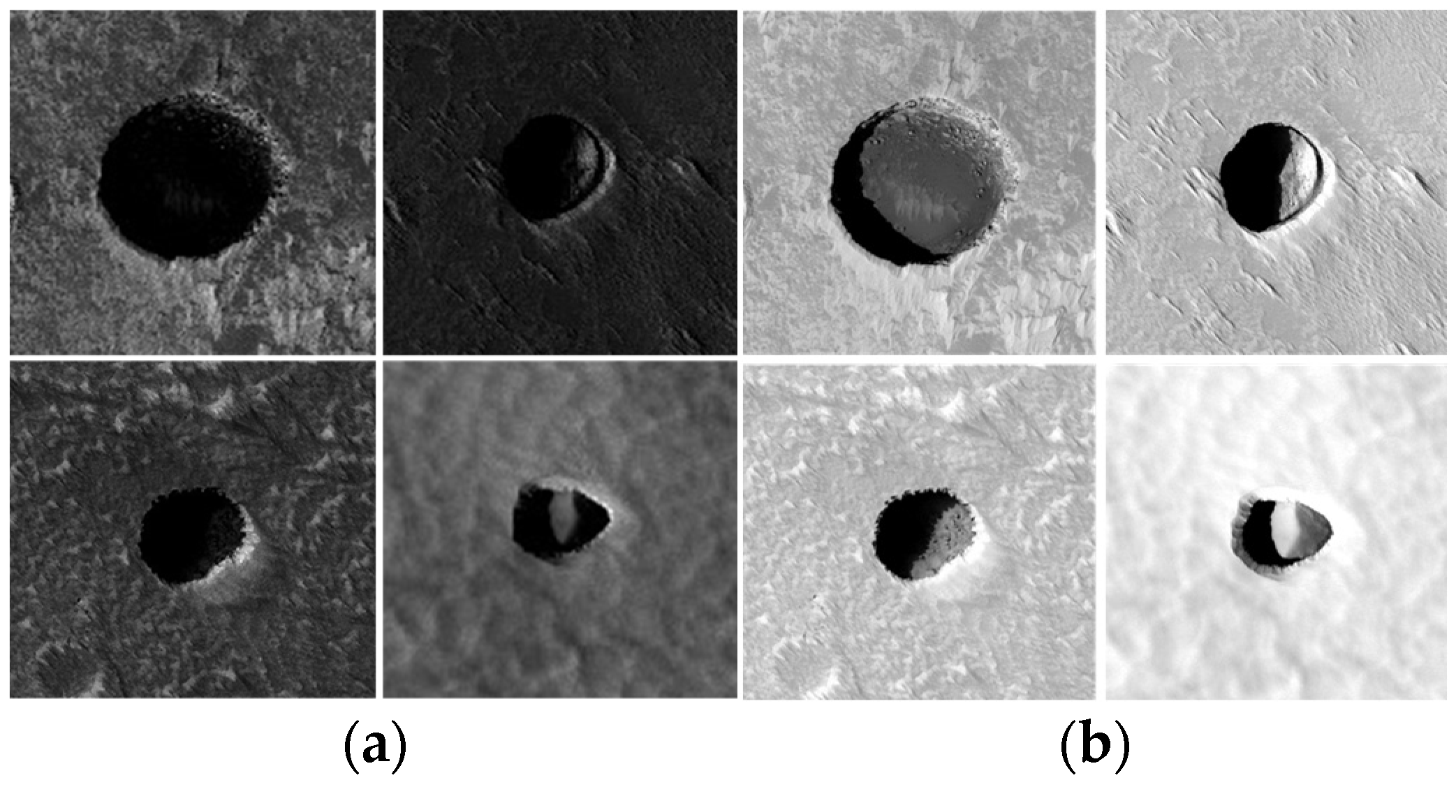
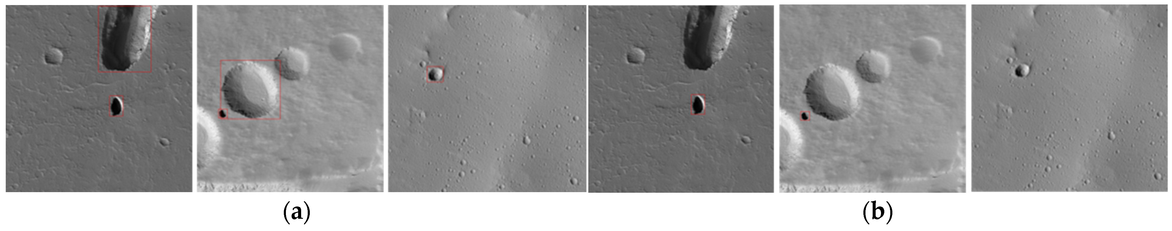
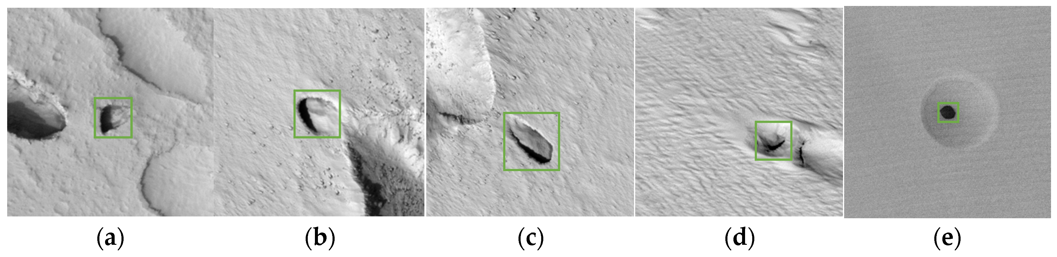
Although there are some identified skylights by manual identification (as summarized in the introduction), they had positional offset and low accuracy. Figure 2 shows some identified examples by Cushing, Sharma & Srivastava, and Tettamanti using MRO-CTX image data. In Figure 2a,b, there is evident positional offset between the labels made by Cushing et al. and Tettamanti. Meanwhile, in Figure 2c, Sharma & Srivastava misidentified some skylights without overhanging or vertical walls. So, it is impossible to build a skylight dataset based on those existing identification results directly. But the results provide the georeferenced information, which can be used to locate skylights and accelerate labeling samples to create a new sample dataset. So, the skylights identified by Cushing, Sharma & Srivastava and Tettamanti in the experimental areas were selected as the georeferenced data.

MO-THEMIS, MRO-CTX, and MRO-HiRISE image data has been used to identify skylights, with resolutions of 100 m/pixel, 6 m/pixel, and 0.25 m/pixel respectively. MO- THEMIS daytime image coverage is global, while the nighttime image coverage spans from 60°S to 60°N, and MRO-CTX and MRO-HiRISE image data covers 99.1% and 1% of the surface of Mars, respectively [20,21].

Table 1. Spatial resolution and coverage rate of MO-THEMIS, MRO-CTX, and MRO-HiRISE image data.

Mission	Sensor	Spatial Resolution	Coverage Rate
MO (USA, 2001.4)	THEMIS	100 m/pixel	Daytime: global; nighttime: latitudes from 60°S to 60°N
MRO (USA, 2005.8)	CTX	6 m/pixel	99.1%
MRO (USA, 2005.8)	HiRISE	0.25 m/pixel	1%

shows the spatial resolution and coverage rate of MO-THEMIS, MRO-CTX, and MRO-HiRISE image data. Since the radii of the observed skylights are small (<112.5 m) [22], some morphological details cannot be imaged in relatively low-resolution image data such as MRO-CTX and MO-THEMIS images. To get more subtle features of the skylight, high-resolution image data is required. Meng et al. [23] suggested that the detected crater is reliable when the diameter exceeds 10 pixels in the image. According to the above suggestion, the diameter of the identified skylights, as the same negative landform, should be more than 10 pixels. The diameter of the minimal identified skylight is 5 m [24], so the resolution should be higher than 0.5 m/pixel (5 m ÷ 10 pixel = 0.5 m/pixel). At present, MRO-HiRISE images are the only data whose resolution (0.25 m/pixel) meets the above requirement. Therefore, MRO-HiRISE image data was selected as the data resource (https://www.uahirise.org/hiwish/browse (accessed on 20 January 2024)) to build the dataset in this article. And 3607 images were downloaded in the experimental areas.

The MRO-HiRISE images were acquired with different levels of illumination, which may make the characteristics of images not obvious. Some experiments have shown that image stretching can highlight the morphological characteristics and enhance the object detection accuracy [25]. In this article, the max-min stretching method (Equation (1)) was selected to stretch the images. Figure 3 shows some images before and after stretching. In the stretched images, the characteristics of the skylights are enhanced and become obvious.

$$x_{new}={\displaystyle \frac{x_{input}-x_{min}}{x_{max}-x_{min}}}\times 255$$

(1)

2.3. Initial Dataset Building

A skylight identification model should require sufficient skylight samples for effective training, which enables the model to learn enough features and achieve robust identification performance. However, the existing skylight identification results have shown that identified Martian skylight samples are few. If those samples were used to train the identification model, it would affect the identification performance. As described in the introduction, it is necessary to build an initial dataset to augment the dataset. Building an initial dataset includes labeling samples and cropping data.

• Labeling Samples

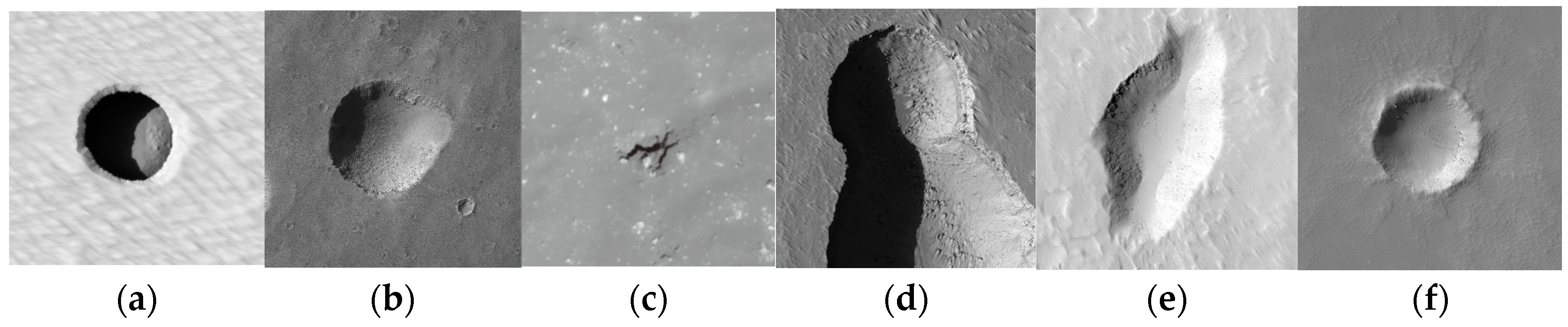
In addition to skylights, there are also some other similar types of negative landforms on Mars, such as bowl-shaped pits, fracture pits, irregular-shaped pits, and craters, as shown in Figure 4. The morphological similarities probably pose a challenge in distinguishing skylights from other negative landforms using deep learning models. To address the problem, some researchers have introduced some negative samples into the dataset [26,27]. The negative samples provide distracted characteristics distinct from the positive samples, which can enable the model to mitigate overreliance on localized patterns of positive samples and instead learn discriminative global features. Therefore, in this article, skylights are labeled as positive samples and other negative landforms labeled as negative samples. Meanwhile, to enable the model to learn diverse distracted characteristics, negative samples should be labeled as diversely as possible.

During labeling samples, it is necessary to record the boundary of samples. In the experiment, the geographical information system software ArcMap 10.2 was used to label the boundary of sample with the stretched MRO-HiRISE images. Sample labeling includes the following steps:

(1) Create a shapefile and set its coordinate projection system consistent with the corresponding MRO-HiRISE image.

(2) Use the georeferenced skylight to search, locate, and label the corresponding skylight in the stretched image. Because there is a spatial offset between the georeferenced skylight and the corresponding skylight in the enhanced image (due to the spatial offset between MRO-CTX and MRO-HiRISE images), it is necessary to manually identify and confirm the corresponding object. After confirming, a circle was used to label the skylight. For the negative samples, we labeled some classic bowl-shaped pits, fracture pits, irregular-shaped pits, and craters.

(3) Merge all the labeled samples and output the location and radii. In the ArcMap, we used the Arc Toolbox to merge the identified samples in one file and used the “Calculate Geometry” function to get the radius and coordinate of the center point for each sample.

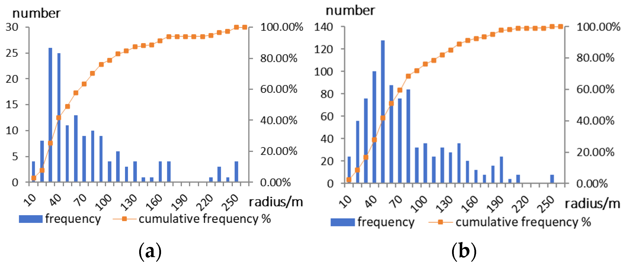
Finally, we labeled 151 skylight samples manually. Most of their radii are less than 100 m, and none exceeds 250 m (see Figure 5a). Meanwhile, we labeled 920 negative samples with a radius < 250 m (see Figure 5b).

2.

Cropping Data

In the following experiments, about 115 positive samples and 920 negative samples are used for augmenting positive samples for identification model building. To ensure the integrity of the sample, the cropped block must fully cover the range of the sample. As shown in Figure 5, the largest radius of the sample is about 250 m, so the minimum side length of the image block is about 2048 pixel (2 × 250 m ÷ 0.25 m/pixel = 2000 pixel ≈ 2048 pixel). In this article, the target-centered cropping method was used to crop the HiRISE image. For each sample, the localization was based on the center point. And then, the corresponding image block was cropped by 2048 pixel × 2048 pixel.

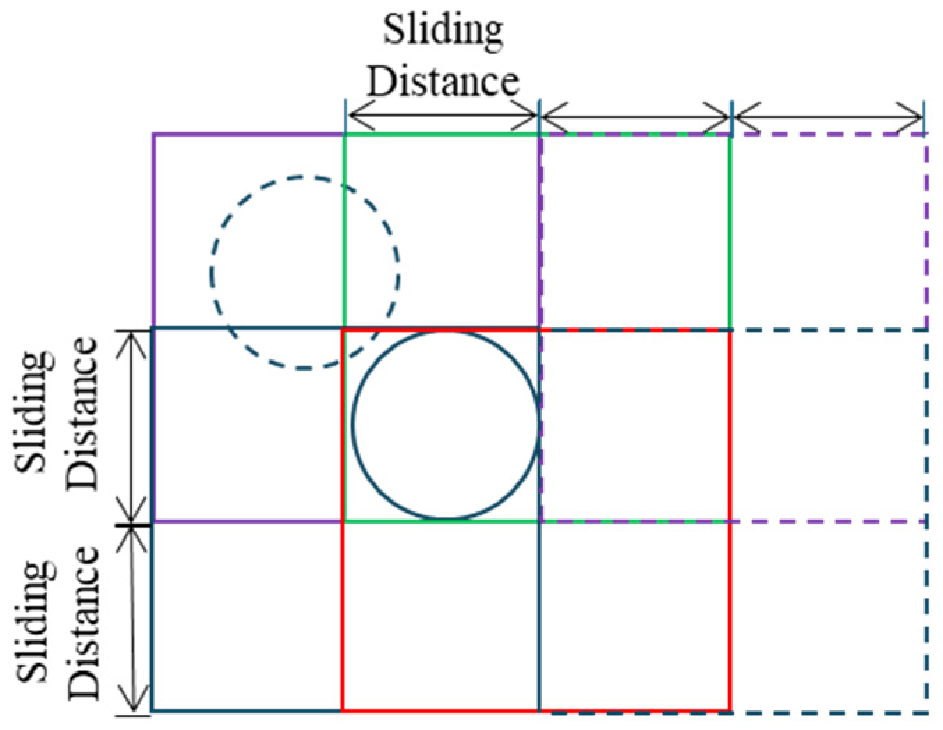
To evaluate the performance of identification model, the other 36 positive samples in 36 MRO-HiRISE images were selected to create a test dataset. In addition, to test the model’s robustness in filtering out false positives within real-world scenarios, the test dataset should introduce distractors (other negative landforms and backgrounds). To reserve the above information for the test samples, the sliding window method was used to crop the 36 MRO-HiRISE images. During the cropping process, the minimum side length of sample is 2048 pixels (calculation process as described above) and the sliding distance is the same as the minimum side length. In the test dataset, the largest sample should be covered by at least an image block. So, the image block is defined as 4096 pixel × 4096 pixel (see Figure 6). For each MRO-HiRISE image file, the image was cropped by 4096 pixel × 4096 pixel, with a 2048 pixel sliding distance from left to right and top to bottom.

After cropping the data, we obtained the initial dataset, which contained 115 positive sample image blocks and 920 negative sample image blocks for data augmentation, and 6394 image blocks (including 36 positive samples along with other negative landforms and background regions) for identification model testing.

3. Data Augmentation

In the initial dataset, the number of positive samples was very small. If the initial dataset was used to build the identification model, the identification accuracy would be low. So, it was necessary to augment the initial dataset with effective generated positive samples. Data augmentation can be achieved by basic image manipulation techniques and generative models [28]. Samples generated by basic image manipulations (such as rotation, cropping, and scaling) are often too similar to the initial samples, which cannot effectively enrich the initial dataset and enhance the model’s identification capability and may even lead to overfitting [29]. As described in introduction, Nodjoumi et al. [16] employed this data augmentation method, but it did not improve the identification performance for Martian negative landforms. However, synthetic samples by generative models offer diverse semantic content which enriches the initial dataset and enhances the model’s robustness. So, in this article, we synthesized samples by generative models to augment the initial dataset.

3.1. Synthesizing Positive Samples with Different Generative Models

In this article, we selected three mainstream generative models—Variational Autoencoder (VAE), StyleGAN2-ADA, and Stable Diffusion—to synthesize positive samples [30]. The following steps are for synthesizing positive samples.

Firstly, prepare the training data. Synthesizing positive samples is based on 115 initial positive samples. Because VAE, StyleGAN2-ADA, and Stable Diffusion are unsupervised generative models, their training data needs to be unlabeled. Therefore, we retained positive samples without labels.

Secondly, build generative models. The positive sample image blocks were used to train the above generative models. For VAE, it was trained using the Stochastic Gradient Descent (SGD) optimizer. The training was conducted for 1000 epochs with a batch size of 8. The noise vector dimension was set to 100, and the learning rate was set to 10⁻⁴. As for StyleGAN2-ADA, the above positive sample images were first converted into compressed format using the StyleGAN2-ADA dataset preprocessing toolkit. These compressed images were then used to train the model. The training was configured with a total of 1000 kimg, adaptive data augmentation (ADA), a batch size of 4, and the evaluation metric set to FID50k_full. The model was optimized using the SGD optimizer. In the case of Stable Diffusion, it was fine-tuned with low-rank adaptation during training, which updated only a subset of the parameters to reduce computational costs. Additionally, data augmentation was performed through random flipping. The training was conducted with a rank of 16 for 10 epochs, a batch size of 2, and a learning rate of 10⁻⁴, using the Adam optimizer.

Thirdly, synthesize positive sample images. For VAE, positive sample images were directly synthesized using the pre-trained VAE model. As for StyleGAN2-ADA, the pre-trained model was used to synthesize positive sample images. During the process, the truncation parameter controls the similarity between synthesized images and the training data distribution. To optimize morphological diversity while preserving the essential characteristics of skylights, ψ was set to 0.7. The noise mode was set to constant mode. In the case of Stable Diffusion, positive sample images were synthesized using the pre-trained Stable Diffusion model, with number_inference_steps set to 8 and guidance_scale_configured to 7.5. Considering the need to add a certain number of synthetic samples to the initial dataset, 1000 images of positive samples for each generative model were synthesized temporarily.

Finally, label these image blocks with the boundary of the skylights. We created labels for each image block by recording the size and position of the skylight in each image block. Therefore, synthetic positive samples were obtained.

Figure 7 shows these initial positive samples and synthetic positive samples. The synthetic positive samples generated by VAE demonstrate the lowest clarity, irregular boundary, and lack diversity in the skylights and background. The synthetic positive samples generated by StyleGAN2-ADA are closer to the initial positive samples, showing better clarity and fidelity, though with moderate diversity. The positive samples synthesized by Stable Diffusion exhibit the highest clarity and diversity, with medium fidelity of the skylights and background.

3.2. Optimal Synthetic Positive Sample Type Selection

After positive sample synthesizing, we obtained three types of synthetic positive samples. It is necessary to select the optimal one with a suitable evaluation method. Visual evaluation is simple and direct, but subjective, so we should evaluate them according to their performance in skylight identification. The traditional evaluation method typically involves augmenting the initial datasets, then comparing the identification accuracy changes before and after the augmentation [31,32]. Therefore, this method introduces two variables, the quantity of samples and the type of synthetic samples, which make it complicated to find the resulting fluctuation factor. However, the Hybrid Recognition Score (HRS) evaluation method keeps the total number of samples in the dataset constant while only changing the type of synthetic samples [17], thereby evaluating the quality of synthetic samples objectively. So, we used the HRS method to evaluate the three types of synthetic positive samples and select the optimal one.

The HRS method requires training of skylight identification models based on the datasets of three types of synthetic positive samples, evaluating the identification accuracy of these models, and then the synthetic positive sample type corresponding to the identification model with the highest accuracy is the optimal one. Therefore, to evaluate the quality of these synthetic positive samples by the HRS method, an appropriate skylight identification model is needed. The YOLO models have been used to identify the negative Martian landforms [15,33]. YOLOv9 [34], as one of the latest YOLO models, was used to build the skylight identification model. So, we conducted an experiment to train YOLOv9 separately on datasets containing different types of synthetic positive samples, evaluate the identification accuracy using the F1 score, and select the best one as the optimal synthetic positive sample type. The following steps are for selecting the optimal synthetic positive sample type.

Firstly, we used the initial dataset and the synthetic positive samples to create four new datasets, of which the former three contained synthetic samples and the initial samples, and the last one contained only the initial samples. Each of the former three datasets included 10 subsets. In 10 subsets, the Hybrid Rate (HR, defined as in Equation (2)) value changed from 10% to 100% with a step of 10% of the quantity of initial positive samples. When reducing the initial positive samples, synthetic positive samples were increased. They were randomly selected from 1000 synthetic samples per type (Section 3.1). Meanwhile, in 10 subsets, the total number of samples remained constant and the numbers of positive and negative samples were equal. Negative samples were randomly selected from the 920 negative samples (Section 2). Ten subsets of each type are shown in

Table 2. Ten subsets of three types of synthetic positive samples.

HR	Synthetic Positive Samples	Initial Positive Samples	Negative Samples	Total Samples
10%	12	103	115	230
20%	23	92	115	230
30%	35	80	115	230
40%	46	69	115	230
50%	58	57	115	230
60%	69	46	115	230
70%	81	34	115	230
80%	92	23	115	230
90%	104	11	115	230
100%	115	0	115	230

. This process generated 30 subsets. Assigning the dataset containing only the initial samples as the 31^st subset, there were 31 subsets in total.

$$\mathrm{H}\mathrm{R}={\displaystyle \frac{\mathrm{N}\mathrm{u}\mathrm{m}\mathrm{b}\mathrm{e}\mathrm{r} \mathrm{o}\mathrm{f} \mathrm{S}\mathrm{y}\mathrm{n}\mathrm{t}\mathrm{h}\mathrm{e}\mathrm{t}\mathrm{i}\mathrm{c} \mathrm{P}\mathrm{o}\mathrm{s}\mathrm{i}\mathrm{t}\mathrm{i}\mathrm{v}\mathrm{e} \mathrm{S}\mathrm{a}\mathrm{m}\mathrm{p}\mathrm{l}\mathrm{e}\mathrm{s}}{\mathrm{N}\mathrm{u}\mathrm{m}\mathrm{b}\mathrm{e}\mathrm{r} \mathrm{o}\mathrm{f} \mathrm{T}\mathrm{o}\mathrm{t}\mathrm{a}\mathrm{l} \mathrm{P}\mathrm{o}\mathrm{s}\mathrm{i}\mathrm{t}\mathrm{i}\mathrm{v}\mathrm{e} \mathrm{S}\mathrm{a}\mathrm{m}\mathrm{p}\mathrm{l}\mathrm{e}\mathrm{s}}}$$

(2)

Then, each of the 31 subsets was individually used to train YOLOv9, thereby building 31 skylight identification models.

Finally, the 31 skylight identification models were tested with the test dataset to obtain the identification accuracy. In addition, identification accuracy curves were plotted based on identification accuracies at different HRs of three types of synthetic positive samples.

Table 3. The identification accuracy at different HRs of three synthetic sample types.

	Type	VAE	StyleGAN2-ADA	Stable Diffusion
HR
0%		73.8%	73.8%	73.8%
10%		72.3%	71.9%	73.3%
20%		71.5%	71.7%	72.7%
30%		71.2%	71.9%	71.4%
40%		71.1%	71.4%	70.9%
50%		71.1%	70.8%	71.1%
60%		70.4%	71.7%	70.4%
70%		56.4%	71.1%	69.6%
80%		56.1%	69.7%	67.4%
90%		48.9%	69.6%	59.4%
100%		44.4%	68.1%	57.1%

and Figure 8 show the identification accuracy and corresponding accuracy curves for the three types of synthetic positive samples at different HRs. In Figure 8, when HR = 0 (only initial samples are used), the identification accuracy achieves the peak value of 73.8%. As the HR increases, the accuracy declines. When HR ≤ 60%, the accuracy drops slowly but remains above 70%. However, when HR > 60%, the identification accuracy corresponding to VAE drops sharply and decreases from 70.4% to 44.4%. When HR > 80%, the identification accuracy corresponding to Stable Diffusion also decreases rapidly. Overall, it can be seen that the identification accuracy corresponding to VAE shows the fastest decline, while the identification accuracy corresponding to StyleGAN2-ADA performs relatively stably. Therefore, the synthetic positive samples generated by StyleGAN2-ADA were selected as the optimal synthetic sample type and used to augment the initial dataset.

3.3. Augmented Dataset Building

There are some differences in the sample characteristics between synthetic positive samples and the initial positive samples. If excessive numbers of synthetic samples were used to augment the initial dataset, the synthetic samples may distort the characteristics of the initial samples, amplifying errors and impairing model performance [35]. So, it is crucial to find the optimal ratio of synthetic positive samples to initial positive samples, which is defined by the Synthetic-to-Initial Ratio (SIR, defined as in Equation (3)) in this article.

$$\mathrm{S}\mathrm{I}\mathrm{R}={\displaystyle \frac{\mathrm{N}\mathrm{u}\mathrm{m}\mathrm{b}\mathrm{e}\mathrm{r} \mathrm{o}\mathrm{f} \mathrm{S}\mathrm{y}\mathrm{n}\mathrm{t}\mathrm{h}\mathrm{e}\mathrm{t}\mathrm{i}\mathrm{c} \mathrm{P}\mathrm{o}\mathrm{s}\mathrm{i}\mathrm{t}\mathrm{i}\mathrm{v}\mathrm{e} \mathrm{S}\mathrm{a}\mathrm{m}\mathrm{p}\mathrm{l}\mathrm{e}\mathrm{s}}{\mathrm{N}\mathrm{u}\mathrm{m}\mathrm{b}\mathrm{e}\mathrm{r} \mathrm{o}\mathrm{f} \mathrm{I}\mathrm{n}\mathrm{i}\mathrm{t}\mathrm{i}\mathrm{a}\mathrm{l} \mathrm{P}\mathrm{o}\mathrm{s}\mathrm{i}\mathrm{t}\mathrm{i}\mathrm{v}\mathrm{e} \mathrm{S}\mathrm{a}\mathrm{m}\mathrm{p}\mathrm{l}\mathrm{e}\mathrm{s}}}$$

(3)

To determine the optimal SIR and obtain the augmented dataset, we created new datasets with different SIRs. Each new dataset covered all the 115 initial positive samples. If the identification model trained by a certain new dataset had the highest identification accuracy, the corresponding SIR would be the optimal ratio, and this new dataset would be the final augmented dataset. The process includes the following steps.

Firstly, create new datasets using the initial samples and the synthetic positive samples. Each dataset contained 115 initial positive samples, some synthetic positive samples, and negative samples. The number of the synthetic positive samples was decided by the SIR and the initial positive samples, and the SIR increased from 0% to 650% with a SIR step of 50%. The number of negative samples was equal to the total number of initial positive samples and synthetic positive samples. So, 14 new datasets were created, as shown in

Table 4. New datasets created at different SIRs (<650%).

SIR	Synthetic Positive Samples	Initial Positive Samples	Negative Samples	Total Samples
0%	0	115	115	230
50%	57	115	172	344
100%	115	115	230	460
150%	172	115	287	574
200%	230	115	345	690
250%	287	115	402	804
300%	345	115	460	920
350%	402	115	517	1034
400%	460	115	575	1150
450%	517	115	632	1264
500%	575	115	690	1380
550%	632	115	747	1494
600%	690	115	805	1610
650%	747	115	862	1724

.

Secondly, train identification models using the new datasets and obtain the identification accuracies. As described in Section 3.2, YOLOv9 was selected as the identification model. As a result, 14 identification accuracies were obtained, based on the above 14 new datasets and the corresponding models.

Thirdly, determine the augmented dataset. The augmented dataset was decided by the highest accuracy.

Table 5. Identification accuracies at different SIRs (<650%).

SIR	Accuracy	SIR	Accuracy
0%	73.80%	350%	84.90%
50%	79.00%	400%	85.30%
100%	84.20%	450%	84.60%
150%	84.60%	500%	84.30%
200%	85.00%	550%	84.20%
250%	85.30%	600%	83.80%
300%	86.80%	650%	83.80%

and Figure 9 show the identification accuracies and corresponding accuracy curve at different SIRs (<650%). In the figure, when SIR = 0, the identification accuracy is lowest (73.8%). As the SIR increases, the identification accuracy improves significantly and then stabilizes. When SIR = 300%, the highest identification accuracy is 86.8%. However, the highest accuracy does not indicate that the optimal SIR is exactly 300% but rather suggests that the identification performance is likely better when the SIR falls within 250~350%.

To further determine the specific optimal SIR and obtain the corresponding augmented dataset, nine new datasets were built with a SIR step of 10%. Using the same method mentioned in the second step, nine identification accuracies were obtained. Figure 10 shows the identification accuracy curve at different SIRs (250~350%). When SIR = 290%, the identification accuracy peaks at 86.9%, which is 13.1% higher than that of SIR = 0. Therefore, 290% is the optimal SIR, and the corresponding dataset is the augmented dataset.

In the augmented dataset, there are 115 initial positive samples, 333 synthetic positive samples from StyleGAN2-ADA, and 448 negative samples. To train the skylight identification model and fine-tune its hyper-parameters (externally configured variables before model training), the augmented dataset was divided into the training dataset and validation dataset at a ratio of 10:1.

4. Identification Methods

4.1. Building a Skylight Identification Model Based on YOLOv9

• YOLOv9

In this article, YOLOv9 was used as a baseline framework for skylight identification.

As shown in Figure 11, YOLOv9’s architecture comprises four main components: the input module, backbone, neck, and prediction head. In the input module, YOLOv9 incorporates data augmentation strategies, including Mosaic, MixUp, and flipping, to enhance the model’s detection performance in complex backgrounds and across varying object scales [36]. In the backbone, YOLOv9 adopts Generalized Efficient Layer Aggregation Network (GELAN) as its core architecture. GELAN ensures efficient feature extraction and preserves key information across layers, thereby achieving a balance between accuracy and computational cost. In the neck, YOLOv9 utilizes programmable gradient information (PGI) to significantly improve feature fusion and mitigate information loss during model training. In the prediction head, benefiting from the invertibility of PGI, YOLOv9 ensures the preservation of critical information during both forward and backward propagation, leading to more reliable and accurate predictions [34]. Overall, by optimizing feature extraction and training strategies, YOLOv9 achieves robust performance in complex and multi-scale object detection scenarios.

2.

Improving Loss Function

Because skylights and other negative landforms may exhibit some variations in shape and size, and often show minimal contrast with the surrounding background, accurate localization is particularly critical for reliable identification. YOLOv9 employs Complete Intersection over Union (CIoU) loss, where the width and height gradients are opposites. This loss function prevents the bounding box’s width and height adjusting simultaneously, possibly resulting in low prediction accuracy of skylights and other negative landforms. Moreover, CIoU loss calculates aspect ratio differences to optimize width and height indirectly, rather than directly reducing the width and height errors between the predicted box and the ground truth box, which leads to slow convergence.

To enhance the bounding box loss function, CIoU loss was replaced by Inner-EIoU (Inner Efficient Intersection over Union) loss. EIoU loss [37] improves upon CIoU loss by separating the influencing factors of the aspect ratio penalty term and independently computing the width and height differences of the predicted and ground truth boxes. This modification allows simultaneous adjustment of the predicted box’s dimensions to minimize the gap between the predicted box and ground truth box. EIoU loss possibly demonstrates superior shape characterization for skylights and other negative landforms, thereby accelerating convergence and improving localization accuracy. The EIoU loss function is shown in Equation (4)

$$L_{EIoU}=1-IoU+{\displaystyle \frac{{\rho }^2\left(b,b^{gt}\right)}{{\left(w^c\right)}^2+{\left(h^c\right)}^2}}+{\displaystyle \frac{{\rho }^2\left(w,w^{gt}\right)}{{\left(w^c\right)}^2}}+{\displaystyle \frac{{\rho }^2\left(h,h^{gt}\right)}{{\left(h^c\right)}^2}}$$

(4)

where IoU represents the intersection over union between the predicted box and ground truth box. b and $b^{gt}$ represent their center points. w and $w^{gt}$ represent their widths. h and ${\mathrm{h}}^{\mathrm{g}\mathrm{t}}$ represent their heights. ${\rho }^2$ indicates the Euclidean distance, and $w^c$ and $h^c$ represent the width and height of the minimal enclosing box which covers both the predicted box and the ground truth box.

Inner-EIoU loss enhances EIoU loss by introducing auxiliary bounding boxes (inner predicted box and inner ground truth box) to accelerate convergence. As shown in Figure 12, the inner predicted box and the predicted box, as well as the inner ground truth box and the ground truth box, differ only in scale. Through comparative experiments, Zhang H. et al. [38] demonstrated that Inner-EIoU, by employing a scale factor to generate auxiliary bounding boxes of different sizes, improves the model’s feature learning efficiency and helps prevent overfitting. Inner-EIoU loss is defined in Equation (5), where ${IoU}^{inner}$ represents the intersection over union for the inner predicted box and inner ground truth box.

$$L_{Inner-EIoU}=L_{EIoU}+IoU-{IoU}^{inner}$$

(5)

3.

Upsampling improving

In skylight identification, upsampling is the key to restoring feature resolution. YOLOv9 uses nearest neighbor interpolation for upsampling. But nearest neighbor interpolation upsampling does not optimize for specific features, which is simple but lacks flexibility. Nearest neighbor interpolation upsampling makes it difficult for the model to effectively extract their details, which may impair the model’s discriminative ability when distinguishing skylights from other negative terrains that share similar local features. Therefore, it is also necessary to improve YOLOv9’s upsampling.

In this article, nearest neighbor interpolation upsampling was replaced by DySample [39] in YOLOv9. DySample redefines the upsampling process from the perspective of point sampling. The process involves creating a sampling set $\mathcal{S}$ via a sampling point generator and then resampling the input feature $\mathcal{X}$ using a grid sampling function to obtain the upsampled feature ${\mathcal{X}}^{\prime }$, as shown in Figure 13. For the sampling point generator, the static scope factor method was adopted. It is the sum of the original grid position $\mathcal{G}$ and the generated offset $\mathcal{O}$, which combines a linear layer and pixel shuffling technology, as shown in Figure 14. Compared with the original upsampling, DySample generates content-aware sampling points, adapting to the input data of multiple negative landforms. Therefore, DySample promotes extracting richer image features, possibly leading to enhanced ability to distinguish skylights and other negative landforms. YOLOv9 incorporating DySample is shown in Figure 15. In this article, the improved YOLOv9 is named YOLOv9-Skylight.

4.2. Model Training and Testing

YOLOv9-Skylight was trained and fine-tuned using the augmented training dataset and validation dataset (see Section 3). During model training, the batch size was set to 16, the number of training epochs was 100, and the input image size was set to 2048 × 2048 pixel. The Stochastic Gradient Descent (SGD) optimizer was employed to minimize the loss function and update the model parameters. The confidence threshold was set to 0.5, meaning that when the predicted confidence score of a target exceeded 0.5, it was identified as a skylight. The configuration of these hyper-parameters is shown in

Table 6. Training parameter configuration.

Hyper-Parameter	Value
epochs	100
batch size	8
image size	2048
optimizer	SGD
confidence threshold	0.5

.

To accelerate model convergence, a warm-up strategy was adopted. During the warm-up phase, the initial learning rate was set to 0.0001 to prevent gradient oscillations or excessive parameter updates in the early stages of training. In the main training phase, the initial learning rate was set to 0.01 to improve convergence efficiency. The hyper-parameters related to the learning rate are summarized in

Table 7. Learning rate parameter configuration.

Warm-Up Initial Learning Rate	Warm-Up Learning Momentum	Warm-Up Learning Rounds	Initial Learning Rate	Recurrent Learning Rate	Learning Rate Momentum	Weight Decay Factor
0.0001	0.8	3.0	0.01	0.01	0.937	0.0005

. To enhance feature extraction capability from varying windows scales, a multi-scale training strategy was adopted, where the input image size was randomly adjusted every 10 iterations. To enhance sample diversity, the flipping data augmentation technique was employed, while scaling, mixing, and mosaicking were disabled to preserve sample integrity.

After training the model, YOLOv9-Skylight was evaluated with the test dataset, and the evaluation metrics included precision (P), recall (R), and F1.

4.3. Comparing with Other Methods

To evaluate the skylight identification performance of the proposed YOLOv9-Skylight, we conducted a series of comparative experiments with some mainstream deep learning models, which included typical one-stage object detection algorithms such as SSD, DETR, YOLOv5, and YOLOv10, as well as two-stage models like Mask R-CNN and Faster R-CNN. The models above were trained and tested under the same experimental conditions using the augmented training dataset and validation dataset. To ensure fairness and objectivity in the comparison, we fine-tuned the hyper-parameters of each model to maximize their F1 scores.

Table 8. Training hyper-parameters for SSD, DETR, YOLOv5, YOLOv9, YOLOv10, Mask R-CNN, and Faster R-CNN.

Models	Epochs	Batch Size	Image Size	Optimizer	Learning Rate	Momentum
SSD	100	8	2048	SGD	0.002	0.937
DETR	100	8	2048	AdamW	0.001	0.937
YOLOv5	100	8	2048	SGD	0.01	0.937
YOLOv9	100	8	2048	SGD	0.01	0.937
YOLOv10	100	16	2048	SGD	0.01	0.937
Mask R-CNN	100	8	2048	SGD	0.01	0.9
Faster R-CNN	100	8	2048	SGD	0.01	0.9

shows the key training hyper-parameters for each model. After training, each model was evaluated on its skylight identification performance using the test dataset.

5. Results and Discussion

5.1. Ablation Study Results

To analyze the effect of Inner-EIoU loss, DySample, and both of them on YOLOv9 for skylight identification, an ablation study was conducted.

Table 9. Ablation study results (bold indicate the maximum value and underlined indicate the minimum value).

DySample	Inner-EIoU Loss	P	R	F1
✕	✕	90.9%	83.3%	86.9%
✓	✕	84.6%	91.7%	88.0%
✕	✓	96.8%	83.3%	89.5%
✓	✓	100%	86.1%	92.5%

shows the results.

Without any improvement, YOLOv9 was used to identify skylights with F1 = 86.9%. After replacing the upsampling method of YOLOv9, the P decreases by 6.3%, and the R and F1 increase by 8.4% and 1.1%. It indicates that DySample promotes the skylight feature extraction of the model, thereby identifying more skylights. When only the loss function is replaced by Inner-EIoU loss, the P (by 5.9%) increases obviously, while the R remains unchanged and the F1 shows a 2.6% improvement. The result highlights the effectiveness of the new loss function in refining localization capabilities. When both are replaced at the same time, the P (by 9.1%), R (by 2.8%) and F1 (by 5.6%) all increase markedly, which proves the effectiveness of the proposed improvements.

Figure 16 shows the skylights identified by YOLOv9 and YOLOv9-Skylight. For YOLOv9, the model is prone to misidentifying pits with smooth rims as skylights, as shown in the left and middle images of Figure 16a. Moreover, when the shadow pattern of the impact crater at certain illumination angles is similar to the shadow features of the skylight, YOLOv9 misidentifies it as a skylight (as shown in the right-hand image of Figure 16a). However, YOLOv9-Skylight avoids these errors (Figure 16b), demonstrating a significant improvement in distinguishing between skylights and other negative landforms. The identification results highlight YOLOv9-Skylight’s higher accuracy and reliability.

5.2. Comparison of the Results with Other Methods

To further confirm the effectiveness of the improvements for YOLOv9, we compared YOLOv9-Skylight with several typical object detection models (SSD, Faster R-CNN, Mask R-CNN, DETR, and YOLO series) for skylight identification. As shown in

Table 10. The skylight identification results of different methods (bold indicate the maximum value and underlined indicate the minimum value).

Method	P	R	F1
Faster R-CNN	67.4%	80.5%	73.4%
Mask R-CNN	68.2%	83.3%	75.0%
SSD	78.8%	72.2%	75.4%
DETR	87.1%	75.0%	80.6%
YOLOv10	96.3%	72.2%	82.5%
YOLOv5	84.2%	88.9%	86.5%
YOLOv9	90.9%	83.3%	86.9%
YOLOv9-Skylight	100%	86.1%	92.5%

, YOLOv9-Skylight achieves the highest F1 of 92.5%, outperforming both its baseline model YOLOv9 (86.9%) and YOLOv5 (86.5%), with YOLOv9 slightly better than YOLOv5. YOLOv10 and DETR yielded a moderate F1 of 82.5% and 80.6%, respectively. SSD, Faster R-CNN, and Mask R-CNN showed the lowest performance, with F1 ranging from 73% to 76%. These results indicate YOLOv9-Skylight’s better skylight identification capability.

5.3. Missed Identification Samples

Although YOLOv9-Skylight has better skylight identification performance than other object detection models, its identification ability is still limited by the size of the training dataset. The experimental results show that YOLOv9-Skylight failed to identify five skylights with no false identification. As can be seen in Figure 17, these missed skylights mainly exhibit three special morphologies. In Figure 17a–c, the skylights exhibit irregular shapes, differing from most circular or near-circular skylights in the training dataset. In Figure 17d, the walls and the floor of the skylight are not apparent. In Figure 17e, the skylight appears as a small black circle, lacking visible overhanging walls and the floor. The latter two types of skylights were absent from the training dataset. Due to the extremely limited number or complete absence of skylights with these special morphologies in the training dataset, YOLOv9-Skylight possibly failed to sufficiently learn their distinctive features and missed some skylights. Although the training dataset was augmented using StyleGAN2-ADA, the synthetic positive samples did not significantly enhance the diversity of skylight characteristics. So, the skylight identification performance of YOLOv9-Skylight was constrained by the insufficient size and diversity of the training dataset.

6. Conclusions

In this article, we proposed a Martian skylight identification method based on a deep learning model. Due to the lack of a suitable dataset for skylight identification, an initial skylight dataset was created, but it includes few positive samples. To augment the initial dataset, three types of synthetic positive samples generated by VAE, StyleGAN2-ADA, and Stable Diffusion were evaluated by the HRS method to select the optimal one. And an optimal ratio of synthetic positive samples to initial positive samples for building the augmented dataset was determined through comparative experiments. In this article, YOLOv9 was used as the baseline model for identifying skylights. To enhance its localization accuracy and feature extracting ability, YOLOv9 was improved by incorporating Inner-EIoU loss and DySample. After training and testing with the augmented skylight dataset, YOLOv9-Skylight was built. To evaluate the skylight identification performance of the proposed YOLOv9-Skylight, we conducted a series of comparative experiments with some mainstream deep learning models.

The result showed that the data augmentation and model architecture improvement play a significant role in enhancing skylight identification performance. For data augmentation, synthetic positive samples generated by StyleGAN2-ADA were the optimal type, and 290% was found to be the optimal ratio of synthetic positive samples to initial positive samples. Meanwhile, the augmented dataset can be used as the basis for deep learning model construction for skylight identification. As for model architecture improvement, YOLOv9-Skylight achieved a precision of 100%, a recall of 86.1%, and an F1 score of 92.5%. Compared with other mainstream models such as YOLOv5, YOLOv9, YOLOv10, Faster R-CNN, Mask R-CNN, and DETR, YOLOv9-Skylight achieved the highest accuracy, which demonstrated the effectiveness of the proposed improvements.

With the growing availability of high-resolution images of Mars and other extraterrestrial bodies, the Martian skylight identification method proposed in this article can be improved and applied to identifying more skylights, which will be used to study volcanic activity and the evolution of extraterrestrial bodies, and even select exploration targets and the promising potential sites for human habitation in future missions.

In future research, the analysis of skylights’ morphological characteristics and spatial distribution patterns can be further strengthened. Moreover, by integrating existing studies on skylights with knowledge of Martian volcanic activity and magma evolution, a deeper understanding of the formation and evolutionary processes of skylights may be achieved.