A Directional Wave Spectrum Inversion Algorithm with HF Surface Wave Radar Network

Abstract

In high-frequency surface wave radar (HFSWR) systems, the retrieval of the directional wave spectrum has remained challenging, especially in the case of echoes from long ranges with a low signal-to-noise ratio (SNR). Therefore, a quadratic programming algorithm based on the regularization technique is proposed with an empirical criterion for estimating the optimal regularization parameter, which minimizes the effect of noise to obtain more accurate inversion results. The reliability of the inversion method is preliminarily verified using simulated Doppler spectra under different wind speeds, wind directions, and SNRs. The directional wave spectra inverted from a radar network with two multiple-input multiple-output (MIMO) systems are basically consistent with those from the ERA5 data, while there is a limitation for the very concentrated directional distribution due to the truncated second order in the Fourier series. Further, in the field experiment during a storm that lasted three days, the wave parameters are calculated from the inverted directional spectra and compared with the ERA5 data. The results are shown to be in reasonable agreement at four typical locations in the core detection area. In addition, reasonable performance is also obtained under the condition of low SNRs, which further verifies the effectiveness of the proposed inversion algorithm.

1. Introduction

Since the discovery of the Bragg scattering mechanism over the ocean surface by Crombie [1], high-frequency surface wave radar (HFSWR) systems, such as SeaSonde and WERA, have been widely applied for the remote sensing of sea state [2,3]. However, the extraction of the directional wave spectrum remains a considerable challenge due to the highly nonlinear and ill-posed nature of the second-order scattering theory by Barrick and Weber [4]. Considering the directional ambiguity inherent in a single-radar system, a network with at least two radar sites is recommended for accurate measurements of the directional wave spectrum [5]. Nevertheless, the networked radar sites are normally separated by tens of kilometers, resulting in a low signal-to-noise ratio (SNR) of echoes from the common radar cell at long ranges.

In recent decades, researchers including Barrick, Lipa, and Wyatt have made fundamental contributions to the estimation of ocean wave spectra from radar Doppler spectra by using some approximations to the nonlinear integral equation [6,7,8,9,10]. Later, Gill and Howell developed an algorithm based on linearization of the double integral and Fourier expansion of the directional wave spectrum, which was applied not only to narrow-beam radars but also to wide-beam systems [11,12]. In 1996, Hisaki converted the problem of solving the nonlinear integral equation into a nonlinear optimization problem without any linearization or approximation, and some additional constraints were added to obtain a stable solution [13]. In recent years, a variety of inversion methods for different scenarios have emerged [14,15,16,17,18,19,20,21], and even popular artificial neural networks were being considered for the inversion of HF radar Doppler spectra [22]. In general, these inversion methods are divided into two categories, that is, inversion with the linearized version of the second-order equation and inversion without linearization or approximation. The former can only be applied in the Doppler frequency region near first-order peaks due to the approximation conditions, while the latter can improve the inversion accuracy but suffers from time-consuming algorithmic computation. However, few of these existing works have yielded ocean wave spectra at a long distance, especially as far as one hundred kilometers away, where the SNR of the second-order spectrum is relatively low due to the propagation attenuation of electromagnetic waves over the sea surface, resulting in a relatively large deviation for these methods.

In the case of low SNRs, the Doppler frequency region used for the wave spectrum inversion is reduced, which worsens the ill-posed nature of the integral equation and makes the solution of the inversion problem sensitive to noise. Therefore, in this article, a quadratic programming algorithm based on the regularization technique is proposed for the inversion of the directional wave spectrum using radar-received Doppler spectra from long ranges as far as one hundred kilometers away with a low SNR. The linearized version of the Barrick-Weber equation is converted into a system of linear equations by expanding the directional wave spectrum on a function basis. Specifically, the Fourier series expansion is considered in the directional dimension, and then the Lewitt–Kaiser–Bessel (L-K-B) function representation [23,24] is used in the frequency dimension. In order to maintain the stability of the inversion, some constraints are imposed on the variables to be solved, and an empirical criterion for estimating the optimal regularization parameter is given to minimize the effect of noise. Then, a dual-radar experiment was conducted during a storm that lasted three days to verify the effectiveness of the proposed algorithm.

The rest of this article is organized as follows. In Section 2, the theoretical background is introduced, and the proposed inversion method is described in detail. In Section 3, some typical simulations are conducted to demonstrate the reliability of the algorithm, and some inversion results from the Advanced Marine Radar (AMR) network are presented. Finally, a discussion and conclusions are provided in Section 4 and Section 5, respectively.

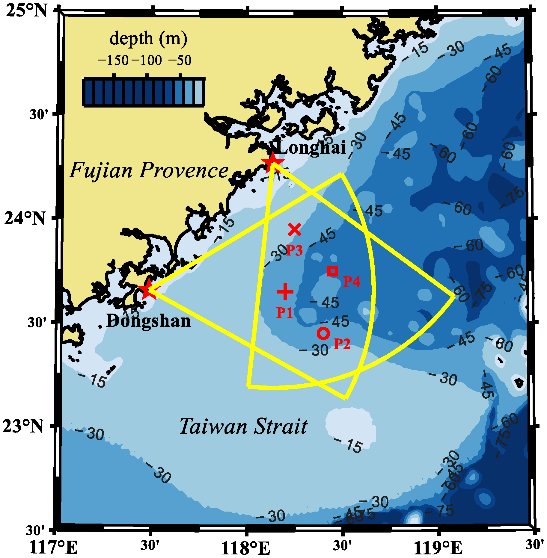
2. Materials and Methods

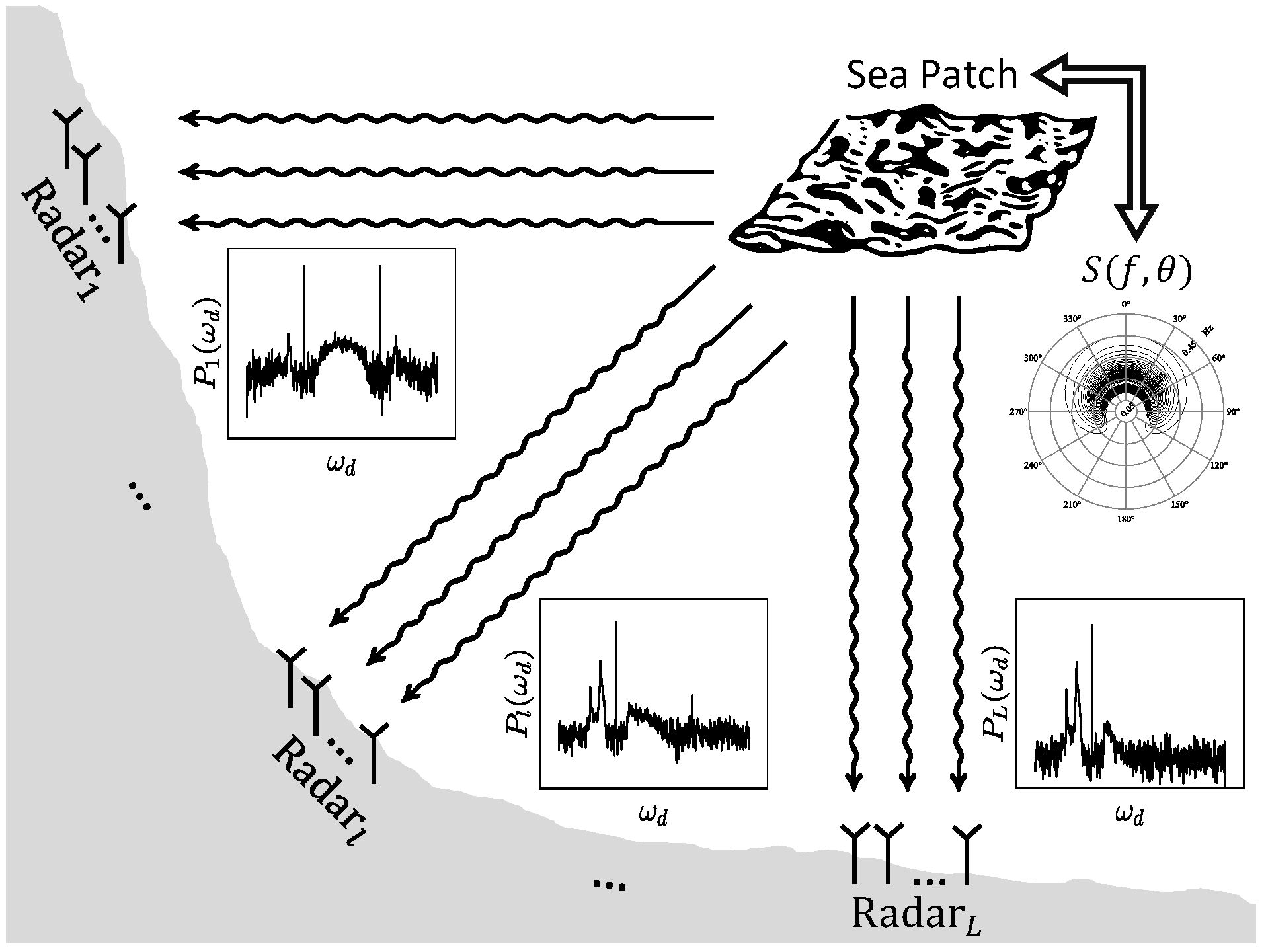
2.1. Problem Formulation and System Model

Electromagnetic waves are emitted by an HF radar system and propagate along the sea surface. They interact with the random, rough surface and are scattered in all directions. Then, the backscattered radio waves are received by an antenna array and converted into digital signals. After a series of signal processing, the Doppler spectrum corresponding to a sea patch is obtained, and this contains a wealth of information about the sea waves. According to Longuet-Higgins [25], the ocean surface is time-varying and random, but it can be well represented by the directional wave spectrum. Meanwhile, the radar-received sea echo is also a random process, and its power spectral density (PSD) is the obtained Doppler spectrum which is in terms of the Doppler angular frequency ${\omega }_d$.

Supposing that there are L radars in the network, we can obtain L Doppler spectra, i.e., $P_1\left({\omega }_d\right)$, …, $P_l\left({\omega }_d\right)$, …, $P_L\left({\omega }_d\right)$, with different radar look directions from the sea patch whose directional wave spectrum is denoted as $S(f,\theta )$, as shown in Figure 1. Therefore, an equation system can be established as follows:

$$\left\{\begin{array}{c}{P}_1\left({\omega }_d\right)=T_1\left\{S(f,\theta )\right\}\\ \dots \\ P_l\left({\omega }_d\right)=T_l\left\{S(f,\theta )\right\}\\ \dots \\ P_L\left({\omega }_d\right)=T_L\left\{S(f,\theta )\right\}\end{array}\right.,$$

(1)

where $T_l\{·\}$, $l=1,2,\dots ,L$, are transformation relations between the Doppler spectra and the corresponding directional wave spectrum, which can be derived through the theory of electromagnetic wave radiation, propagation, and scattering. The inversion problem is to solve the equation system to obtain the accurate directional wave spectrum $S(f,\theta )$ using radar-received Doppler spectra. However, the transformation relation is very complicated, and the Doppler spectrum is affected by many unfavorable factors, such as noise and interference. In the rest of this section, we will derive the transformation relation and then design a method for the inversion of the directional wave spectrum which can be applied in scenarios with low SNRs.

2.2. AMR Radar System

A digital multiple-input multiple-output (MIMO) HFSWR called the AMR system was independently developed by the Radio Oceanography Laboratory of Wuhan University [26,27]. The AMR radar network with two radar sites, which are located in Longhai and Dongshan, about 100 km apart, was deployed on the coast of Fujian Province, China, in August 2021, and it is used for remote observation of the common coverage area shown in Figure 2. Each radar site is equipped with a MIMO array consisting of two monopole transmitting antennas and four monopole receiving antennas, as detailed in the literature [27].

Table 1. Typical parameters of the AMR radar system.

Parameter	Value
Operating frequency range (MHz)	8∼13.5
Average transmitting power (W)	200
Maximum range  (km)	200
Range resolution (km)	5
Doppler sampling interval (s)	0.25
FFT length for Doppler spectra	2048
Wave measurement period (min)	10

lists several typical system parameters of the AMR radar.

In this study, the radar dataset used to verify the proposed wave inversion algorithm was collected during a storm from 10 to 12 October 2021. During this period, the significant wave height gradually increased from 2 m to about 6 m in the first half, and then recovered to 2 m in the second half. For long-distance detection, the radar system operated at a frequency of about 8 MHz in the meantime, and the Doppler spectrum was obtained through FFT with a length of 2048 and a sampling interval of 0.25 s, which requires the time of about 8.5 min. However, we calculated a Doppler spectrum every 5 min with a time overlap of about 3.5 min. After MIMO array signal processing [28,29], the range Doppler (RD) spectra from different directions of arrival were obtained. In order to reduce the statistical uncertainty in Doppler spectra [30,31], we output an averaged Doppler spectrum every 10 min using original Doppler spectra from adjacent times, range cells, and radar beams, which means that 27 such spectra are used for the average. Then, the inversion for the directional wave spectrum was performed with the averaged Doppler spectral data from the two radar sites.

2.3. Radar Cross-Section Equations

Theoretically, the radar-received Doppler spectrum $P\left({\omega }_d\right)$ is related to the sea surface patch, which is located at distances $R_T$ and $R_R$ from the transmitter and receiver, respectively, through the radar equation [32]

$$P\left({\omega }_d\right)={\displaystyle \frac{P_T{G}_T{G}_R{\lambda }^2{F}_T^2{F}_R^{2}A}{{\left(4\pi \right)}^3{R}_T^2{R}_R^2}}\sigma \left({\omega }_d\right),$$

(2)

where $P_T$ is the average transmitting power; $G_T$ and $G_R$ are the transmitting and receiving antenna gains in the direction of the patch; $\lambda$ is the radio wavelength; $F_T$ and $F_R$ are the Norton attenuation factors; A is the area of the surface patch; $\sigma \left({\omega }_d\right)$ is the average radar cross-section per unit area per rad/s bandwidth.

In view of the perturbation method by Rice [33], the total radar cross-section is taken as the sum of each order of radar cross-sections, written as $\sigma \left({\omega }_d\right)={\displaystyle \sum _{i=1}^{\infty }}{\sigma }_i\left({\omega }_d\right)$, where i is the order of scattering. In principle, the first two order components could be enough to account for most of the scattering effects. Barrick et al. [4,32] derived the theoretical first- and second-order radar cross-sections in terms of the directional wave spectrum $S\left(\overrightarrow{k}\right)$ and the radar wavenumber vector ${\overrightarrow{k}}_0$.

The first two order components for narrow-beam radars without regard to surface currents are given as

$${\sigma }_1({\omega }_d)=2^6\pi k_0^4\sum _{m^{\prime }=\pm 1}S\left(m^{\prime }{\overrightarrow{k}}_B\right)\delta \left({\omega }_d-m^{\prime }{\omega }_B\right)$$

(3)

and

$${\sigma }_2({\omega }_d)=2^6\pi k_0^4\sum _{m,m^{\prime }=\pm 1}\int {\int }_{-\infty }^{+\infty }{\left|\mathrm{\Gamma }\right|}^{2}S\left(m\overrightarrow{k}\right)S\left(m^{\prime }{\overrightarrow{k}}^{\prime }\right)\delta \left({\omega }_d-m\omega -m^{\prime }{\omega }^{\prime }\right)dpdq,$$

(4)

where $k_0$ is the magnitude of ${\overrightarrow{k}}_0$; ${\overrightarrow{k}}_B$ is the wavenumber vector of the Bragg wave with frequency ${\omega }_B$, and ${\overrightarrow{k}}_B=-2{\overrightarrow{k}}_0$ for monostatic radars; $\overrightarrow{k}$ and ${\overrightarrow{k}}^{\prime }$ are the wavenumber vectors of two waves with frequencies $\omega$ and ${\omega }^{\prime }$, respectively, which satisfy the Bragg resonance condition $\overrightarrow{k}+{\overrightarrow{k}}^{\prime }={\overrightarrow{k}}_B$. In addition, $\mathrm{\Gamma }$ is the coupling coefficient, which includes the hydrodynamic and electromagnetic components, and its more details can be found in many works, such as [6,34].

For ocean gravity waves, the angular frequency is related to the corresponding wavenumber by the dispersion relationship

$$\omega =\sqrt{gktanh\left(kd\right)},$$

(5)

where g is the acceleration of gravity, and d is the depth of water. In this study, we only focus on the deep-water case, in which the formula is simplified to $\omega =\sqrt{gk}$. The relationship will determine the constraints enclosed in the delta function in (3) and (4), and then different frequency contours in the p-q plane are obtained for each Doppler frequency.

2.4. Linearization of the Second-Order Equation

The second-order expression can be simplified with the following steps [35]. First, the integral is doubled and calculated over the right half of the p-q plane due to its bilateral symmetry. Second, the integral about p and q is transformed into an integral about k and $\theta$ (the magnitude and angle of $\overrightarrow{k}$). Then, the variable substitutions are carried out, i.e., $y=\sqrt{k}$ and $h=m\omega +m^{\prime }{\omega }^{\prime }$. Finally, the double integral reduces to a single integral

$${\sigma }_2\left({\omega }_d\right)=2^8\pi k_0^4{\int }_{-{\theta }_L}^{{\theta }_L}{\left|\mathrm{\Gamma }\right|}^{2}S(m\overrightarrow{k})S(m^{\prime }{\overrightarrow{k}}^{\prime })y^3\left|{\displaystyle \frac{\partial y}{\partial h}}\right|d\theta ,$$

(6)

where the integral is calculated along the frequency contour $h={\omega }_d$, and ${\theta }_L$ is the angle limit determined by the frequency contour boundary in the right half plane. When ${\omega }_d^2\le 2{\omega }_B^2$, ${\theta }_L=\pi$; otherwise, ${\theta }_L=\pi -arccos(2{\omega }_B^2/{\omega }_d^2)$. In addition, $m=1,m^{\prime }=1$ for ${\omega }_d>{\omega }_B$; $m=-1,m^{\prime }=1$ for $0<{\omega }_d<{\omega }_B$; $m=1,m^{\prime }=-1$ for $-{\omega }_B<{\omega }_d<0$; $m=-1,m^{\prime }=-1$ for ${\omega }_d<-{\omega }_B$.

Apparently, the integral expression (6) is a nonlinear equation about the directional wave spectrum, which is very difficult to solve. In general, the wavenumber vector ${\overrightarrow{k}}^{\prime }$, which refers to the ocean wave vector with a shorter wavelength involved in the scattering process, is approximately equal to the Bragg wavenumber vector ${\overrightarrow{k}}_B$ for the second-order Doppler spectra near the Bragg peaks [36]. Hence, this wave of ${\overrightarrow{k}}^{\prime }$ is in the short-wavelength region of the wave spectrum, and its spectral value tends to fall off at a rate proportional to $k^{\prime -4}$ [37]. Then, the approximation is given as follows:

$$S\left(m^{\prime }\overrightarrow{k^{\prime }}\right)\approx S\left(m^{\prime }{\overrightarrow{k}}_B\right){\left({\displaystyle \frac{k_B}{k^{\prime }}}\right)}^4,$$

(7)

which serves well for the Doppler frequency range of $0.6{\omega }_B<\left|{\omega }_d\right|<0.9{\omega }_B$ and $1.1{\omega }_B<\left|{\omega }_d\right|<1.4{\omega }_B$ [12].

From the radar equation in (2), the radar-received Doppler spectrum is affected by a variety of uncertain factors, such as fluctuating transmitted power and path losses. To remove these effects, the second-order Doppler spectrum is divided by the total power of the local first-order Doppler spectrum, which yields the normalized second-order radar cross-section

$${\sigma }_{2N}\left({\omega }_d\right)={\displaystyle \frac{P^{\left(2\right)}\left({\omega }_d\right)}{{\displaystyle {\int }_{\omega ·{\omega }_d>0}{P}^{\left(1\right)}\left(\omega \right)d\omega }}}={\displaystyle \frac{{\sigma }_2\left({\omega }_d\right)}{{\displaystyle {\int }_{\omega ·{\omega }_d>0}{\sigma }_1\left(\omega \right)d\omega }}},$$

(8)

where $P^{\left(i\right)}$ is the ith-order Doppler spectrum corresponding to ${\sigma }_i$, and $i=1,2$. Combining (3), (6), (7), and (8) will yield

$${\sigma }_{2N}\left({\omega }_d\right)={\int }_{-{\theta }_L}^{{\theta }_L}C\left({\omega }_d,\theta \right)S\left(m\overrightarrow{k}\right)d\theta ,$$

(9)

where $C\left({\omega }_d,\theta \right)=4k_B^4{\left|\mathrm{\Gamma }\right|}^2{y}^3\left|\partial y/\partial h\right|/k^{\prime 4}$ is the kernel of the integral. Now, the normalized second-order equation becomes linear about the directional wave spectrum.

2.5. Functional Representation and Matrixing

However, the Formula (9) is an integral equation. In order to achieve the numerical calculation, a function basis with good properties is required here, and then the wave spectrum is expanded on this basis. Since the directional wave spectrum $S\left(\overrightarrow{k}\right)$ is a two-dimensional function in terms of the wavenumber and the direction of propagation, it is natural to perform a Fourier series expansion in the directional dimension, i.e.,

$$S\left(\overrightarrow{k}\right)=\sum _{n=0}^N\left[a_n\left(k\right)cos\left(n\theta \right)+b_n\left(k\right)sin\left(n\theta \right)\right],$$

(10)

where $\theta$ is the angle relative to the radar look direction; N is the truncated order of the Fourier series, which is truncated to the second order in this study; $a_n\left(k\right)$ and $b_n\left(k\right)$ are the corresponding Fourier coefficients in terms of the wavenumber k.

Since the Fourier coefficients are still a continuous function of the wavenumber, a set of basis functions is required for further expansion. In [24], the row-action method achieved a great success using the L-K-B expansion for the vector wavenumber, albeit with an SNR limitation. For the method proposed in the study, the L-K-B expansion for the scalar wavenumber is applied, considering that there is a limitation on the number of variables to be solved. The L-K-B function is symmetrical with respect to the center of control points and transitions smoothly to zero, which is suitable for the expansion here. The expression of the L-K-B function is given as

$$\psi \left(r\right)={\left(1-{\left(r/r_{\max }\right)}^2\right)}^{\nu /2}{I}_{\nu }\left(\alpha \sqrt{1-{\left(r/r_{\max }\right)}^2}\right)/I_{\nu }\left(\alpha \right)$$

(11)

for $r<r_{\max }$, and $\psi \left(r\right)=0$ otherwise. Here, r is the radius parameter, and $r_{max}$ is the maximum radius for nonzero values; $I_{\nu }$ is the $\nu$th-order modified Bessel function, and $\alpha$ is the shape control parameter. For simplicity, the variable y mentioned in (6) is to be sampled as the control points. Then, the basis functions $\psi \left(∥y-y_i∥\right)$ are formed for these control points $y_i$, $i=1,2,...,I$. In this study, the parameters in the L-K-B function are chosen as $\nu =2$, $\alpha =9.2$, $r_{max}=1.78\Delta y$, where $\Delta y$ is the grid spacing of $y_i$. According to the definition $y=\sqrt{k}$, we can get $y={\displaystyle \frac{2\pi }{\sqrt{g}}}f$ for deep-water cases, where g is the acceleration of gravity and f is the wave frequency. Here, we take a uniform grid of $y_i$, with $y_1={\displaystyle \frac{2\pi }{\sqrt{g}}}0.036$, $y_I={\displaystyle \frac{2\pi }{\sqrt{g}}}0.36$, and $I=37$, indicating that the range of wave frequency f is about 0.036∼0.36 which includes the majority of energy in wave spectra. Thus, the Fourier coefficients are further expanded as

$$\{\begin{array}{c}{\displaystyle a_n\left(k\right)=\sum _{i=1}^I{x}_{ni}^a\psi \left(∥y-y_i∥\right)}\hfill \\ {\displaystyle b_n\left(k\right)=\sum _{i=1}^I{x}_{ni}^b\psi \left(∥y-y_i∥\right)},\hfill \end{array}$$

(12)

where $x_{ni}^a$ and $x_{ni}^b$ are the corresponding expansion coefficients. Substituting (10) and (12) into (9) yields the series expression of the normalized second-order equation, i.e.,

$${\sigma }_{2N}\left({\omega }_d\right)=\sum _{n=0}^N\sum _{i=1}^I{\int }_{-{\theta }_L}^{{\theta }_L}C\left({\omega }_d,\theta \right)\psi \left(∥y-y_i∥\right)m^n\left[x_{ni}^{a}cos\left(n\theta \right)+x_{ni}^{b}sin\left(n\theta \right)\right]d\theta .$$

(13)

The Doppler spectrum is then uniformly sampled to obtain sample points ${\sigma }_j={\sigma }_{2N}\left({\omega }_{dj}\right)$, $j=1,2,...,J$. While denoting

$$\{\begin{array}{c}{\displaystyle w_{nij}^a={\int }_{-{\theta }_L}^{{\theta }_L}C({\omega }_{dj},\theta )\psi (\parallel y-y_i\parallel )m^{n}cos\left(n\theta \right)d\theta }\hfill \\ {\displaystyle w_{nij}^b={\int }_{-{\theta }_L}^{{\theta }_L}C({\omega }_{dj},\theta )\psi (\parallel y-y_i\parallel )m^{n}sin\left(n\theta \right)d\theta },\hfill \end{array}$$

(14)

the discretized algebraic equations are formed as

$${\sigma }_j=\sum _{n=0}^N\sum _{i=1}^I\left[w_{nij}^a{x}_{ni}^a+w_{nij}^b{x}_{ni}^b\right],$$

(15)

and can be expressed in the form of a matrix:

$$\mathsf{\sigma }=\mathbf{Wx},$$

(16)

where $\mathsf{\sigma }=({\sigma }_1$, ${\sigma }_2$, $...$, ${\sigma }_J{)}^{\mathrm{T}}$, $\mathbf{x}$=$(x_1$, $x_2$, $...$, $x_I{)}^{\mathrm{T}}$, $x_i$=$(x_{0i}^a$, $x_{1i}^a$, $x_{1i}^b$, $...$, $x_{Ni}^a$, $x_{Ni}^b)$, and ${(·)}^{\mathrm{T}}$ denotes transposition. In addition, the matrix is composed of the weight coefficients in (15), i.e., $\mathbf{W}$=${\left(w_{ij}\right)}^{\mathrm{T}}$, where $w_{ij}$=$(w_{0ij}^a$, $w_{1ij}^a$, $w_{1ij}^b$, $...$, $w_{Nij}^a$, $w_{Nij}^b{)}^{\mathrm{T}}$, and is expanded as follows:

$$\mathbf{W}=\left(\begin{array}{cccc}{w}_{11}^{\mathrm{T}}& w_{21}^{\mathrm{T}}& \dots & w_{I1}^{\mathrm{T}}\\ w_{12}^{\mathrm{T}}& w_{22}^{\mathrm{T}}& \dots & w_{I2}^{\mathrm{T}}\\ ⋮& ⋮& \ddots & ⋮\\ w_{1J}^{\mathrm{T}}& w_{2J}^{\mathrm{T}}& \dots & w_{\mathrm{IJ}}^{\mathrm{T}}\end{array}\right).$$

(17)

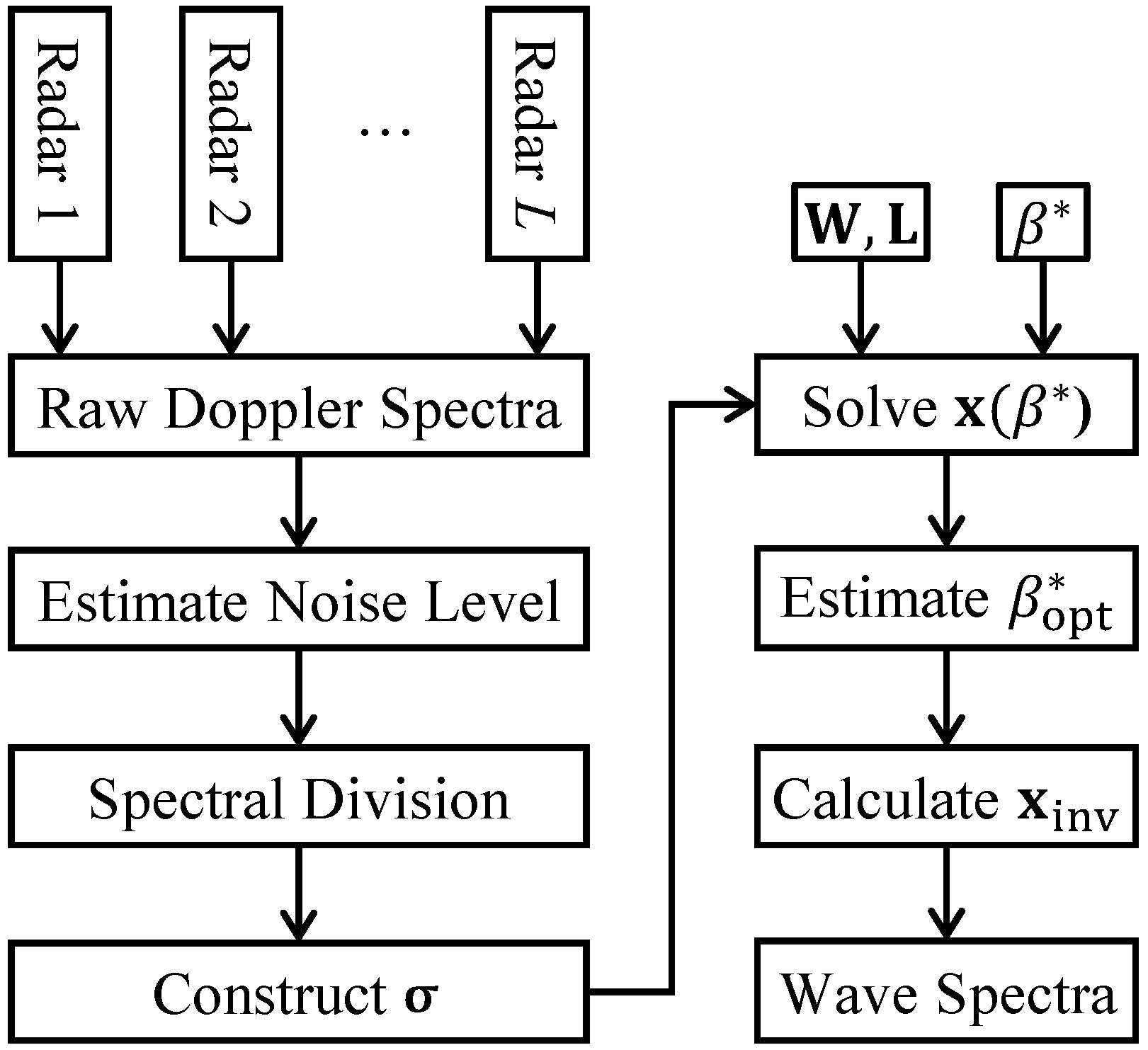
2.6. Inversion with Two or More Radars

For a single-radar system, only the non-directional wave spectrum can be obtained due to the directional ambiguity between waves traveling along the left and right sides of the radar beam, respectively. This problem is normally solved by the use of two or more radars to observe the same sea patch.

In the previous derivation, the reference direction for the directional wave spectrum $S\left(\overrightarrow{k}\right)$ is the radar look direction, which is convenient for processing the single-radar data. However, the look direction of each radar is different for the same ocean surface patch, indicating that a common reference is required for a networked system. Naturally, the geographical coordinate system is a good choice. Then, the expansion (10) is rewritten as

$$S\left(\overrightarrow{k}\right)=\sum _{n=0}^N\left[a_n\left(k\right)cos\left(n\varphi \right)+b_n\left(k\right)sin\left(n\varphi \right)\right],$$

(18)

where $\varphi$ is the direction relative to the true north. For a radar in the network, the geometric relationship is

$$\varphi ={\theta }_R-\theta ,$$

(19)

where ${\theta }_R$ is the radar look direction relative to the true north, and $\theta$ is the angle relative to ${\theta }_R$, as mentioned in (10).

In the geographical coordinate system, the coefficients in (14) are accordingly rewritten as

$$\{\begin{array}{c}{\displaystyle w_{nij}^{a^{*}}={\int }_{-{\theta }_L}^{{\theta }_L}C({\omega }_{dj},\theta )\psi (\parallel y-y_i\parallel )m^{n}cos(n{\theta }_R-n\theta )d\theta }\hfill \\ {\displaystyle w_{nij}^{b^{*}}={\int }_{-{\theta }_L}^{{\theta }_L}C({\omega }_{dj},\theta )\psi (\parallel y-y_i\parallel )m^{n}sin(n{\theta }_R-n\theta )d\theta }.\hfill \end{array}$$

(20)

After simplification, the relationship between these coefficients in the geographical coordinate system and in the radar look direction reference system is obtained as follows:

$$\{\begin{array}{c}{w}_{nij}^{a^{*}}=cos\left(n{\theta }_R\right)w_{nij}^a+sin\left(n{\theta }_R\right)w_{nij}^b\hfill \\ w_{nij}^{b^{*}}=sin\left(n{\theta }_R\right)w_{nij}^a-cos\left(n{\theta }_R\right)w_{nij}^b,\hfill \end{array}$$

(21)

and this can be further denoted as a matrix equation, $w_{ij}^{*}\left({\theta }_R\right)=G\left({\theta }_R\right)w_{ij}$, where

$$G\left({\theta }_R\right)=\left(\begin{array}{cccccc}1& 0& 0& \dots & 0& 0\\ 0& cos\left({\theta }_R\right)& sin\left({\theta }_R\right)& \dots & 0& 0\\ 0& sin\left({\theta }_R\right)& -cos\left({\theta }_R\right)& \dots & 0& 0\\ ⋮& ⋮& ⋮& \ddots & ⋮& ⋮\\ 0& 0& 0& \dots & cos\left(N{\theta }_R\right)& sin\left(N{\theta }_R\right)\\ 0& 0& 0& \dots & sin\left(N{\theta }_R\right)& -cos\left(N{\theta }_R\right)\end{array}\right).$$

(22)

For a networked system with L radars, the matrix equations for each radar can form a larger matrix equation, i.e.,

$$\left[\begin{array}{c}{\mathsf{\sigma }}_1\\ {\mathsf{\sigma }}_2\\ ⋮\\ {\mathsf{\sigma }}_L\end{array}\right]=\left[\begin{array}{c}{\mathbf{W}}_1\\ {\mathbf{W}}_2\\ ⋮\\ {\mathbf{W}}_L\end{array}\right]\mathbf{x},$$

(23)

where ${\mathsf{\sigma }}_l$ is the Doppler spectrum vector from the lth radar, ${\mathbf{W}}_l={\left(w_{ij}^{*}\left({\theta }_{R_l}\right)\right)}^{\mathrm{T}}$ is the corresponding coefficient matrix, and ${\theta }_{R_l}$ is the look direction of the lth radar.

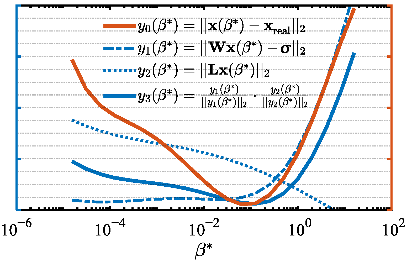
2.7. Equation Constraints and Solution

The solution of (16) or (23) is ill-posed and very susceptible to echo noise, resulting in a biased inversion result. Thus, it is necessary to utilize characteristics of the directional wave spectrum to constrain the vector $\mathbf{x}$ for the stability of the solution. As we know, the wave spectrum has a certain continuity and is non-negative, so the following constraints can be given:

$$\{\begin{array}{c}{\displaystyle S(k_i,{\theta }_d)=\frac{k_{i+1}-k_i}{k_{i+1}-k_{i-1}}S(k_{i-1},{\theta }_d)+\frac{k_i-k_{i-1}}{k_{i+1}-k_{i-1}}S(k_{i+1},{\theta }_d)}\hfill \\ S(k_i,{\theta }_d)\ge 0\hfill \end{array}$$

(24)

where ${\theta }_d=2\pi \left(d-1\right)/D,d=1,2,...,D$. Figure 3 shows the relative error, ${\displaystyle \frac{\Vert {\mathbf{x}}_{\mathrm{inv}}-{\mathbf{x}}_{\mathrm{real}}{\Vert }_2}{\Vert {\mathbf{x}}_{\mathrm{real}}{\Vert }_2}}$, where ${\mathbf{x}}_{\mathrm{inv}}$ is the inversion result and ${\mathbf{x}}_{\mathrm{real}}$ is the real one, vs. D for different second-order peak SNRs in the simulation under a wind speed of 12 m/s and a wind direction of 90°, and the similar trend is maintained under other conditions. As indicated in the figure, the reasonable values of D could take on 12∼36, while the value should be appropriately larger for medium and high SNRs to further reduce inversion errors.

According to the series expansion discussed above, the directional wave spectrum can be expressed as a matrix equation of $\mathbf{x}$, i.e.,

$$S(k,\theta )={\mathbf{p}}^{\mathrm{T}}\left(k,\theta \right)\mathbf{x},$$

(25)

where $\mathbf{p}(k,\theta )$=$(p_1$, $p_2$, $...$, $p_I{)}^{\mathrm{T}}$, $p_i$=$\psi (\parallel y-y_i\parallel )$×$(1$, $cos\left(\theta \right)$, $sin\left(\theta \right)$, $...$, $cos\left(N\theta \right)$, $sin\left(N\theta \right))$. Further, the wave spectrum constraints are also written in the form of a matrix, i.e.,

$$\begin{array}{c}\mathbf{Lx}=\mathbf{0}\hfill \\ \mathbf{Ax}\ge \mathbf{0}\hfill \end{array},$$

(26)

where $\mathbf{L}$=$(L_1$, $L_2$, $...$, $L_I{)}^{\mathrm{T}}$, $L_i$=$(l_{i1}$, $l_{i2}$, $...$, $l_{iD})$, and $l_{id}$=$(k_{i+1}$−$k_i)$$\mathbf{p}(k_{i-1},{\theta }_d)$+$(k_i$−$k_{i-1})$$\mathbf{p}(k_{i+1},{\theta }_d)$−$(k_{i+1}$−$k_{i-1})$$\mathbf{p}(k_i,{\theta }_d)$; $\mathbf{A}$=$(A_1$, $A_2$, $...$, $A_I{)}^{\mathrm{T}}$, and $A_i$=$(\mathbf{p}(k_i,{\theta }_1)$, $\mathbf{p}(k_i,{\theta }_2)$, $...$, $\mathbf{p}(k_i,{\theta }_D))$. Hence, this equality represents the continuity of wave spectra, and the inequality keeps them non-negative as much as possible.

By the definition of the non-directional wave spectrum, its series expression on the function basis is obtained as

$$S\left(k\right)=2\pi a_0\left(k\right)=2\pi \sum _{i=1}^I{x}_{0i}^a\psi \left(∥y-y_i∥\right).$$

(27)

In order to ensure that $S\left(k\right)$ is non-negative everywhere, it could be reasonable to further constrain $x_{0i}^a\ge 0$, considering that $\psi$ is a positive tight support function. In addition, the non-directional wave spectrum is bounded in practice. According to [38], as the wind speed increases, the wave energy at frequencies greater than the peak frequency will enter into a saturated state, and the energy of the wind is almost transferred to the ocean waves of lower frequencies. Therefore, we can take the PM spectrum with a large wind speed as the upper limit for additional constraints. At the ith spectral point, $S\left(k_i\right)\approx 2\pi x_{0i}^a$; then, the constraints $x_{0i}^a\le u_i$ are taken, where $u_i=0.0081exp[-0.74{(k_i{v}_{19.5}^2/g)}^{-2}]/\left(4\pi k_i^4\right)$, and $v_{19.5}$ can take the value of the maximum measurable wind speed of the radar system.

The equality constraint is used as a regular term along with the regularization parameter $\beta$, and then the penalty function is constructed as $F\left(\mathbf{x}\right)=\left|\right|\mathbf{Wx}-{\mathsf{\sigma }\left|\right|}_2^2+{\beta \left|\right|\mathbf{Lx}\left|\right|}_2^2$. Therefore, the solution of the wave spectrum is transformed into an optimization problem, and its simplified version is described as follows:

$$\begin{array}{cc}\hfill \underset{\mathbf{x}}{min}& {\displaystyle \frac{1}{2}{\mathbf{x}}^{\mathrm{T}}\mathbf{Hx}+{\mathbf{f}}^{\mathrm{T}}\mathbf{x}}\hfill \\ \hfill \mathrm{s}.\mathrm{t}.& \mathbf{Ax}\ge 0\hfill \\ \hfill & 0\le x_{0i}^a\le u_i(i=1,2,...,I)\hfill \end{array}$$

(28)

where $\mathbf{H}={\mathbf{W}}^{\mathrm{T}}\mathbf{W}+\beta {\mathbf{L}}^{\mathrm{T}}\mathbf{L}$, and $\mathbf{f}=-{\mathbf{W}}^{\mathrm{T}}\mathsf{\sigma }$. Obviously, this is a quadratic programming problem with linear constraints, and it has been solved by some mature means, such as the interior point algorithm and the active set method.

Before solving the quadratic programming problem, the optimal regularization parameter needs to be determined. Since the optimal value is unknown in advance, it is necessary to iterate through a series of possible values. The regularization parameter $\beta$ is a weight between ${\mathbf{W}}^{\mathrm{T}}\mathbf{W}$ and ${\mathbf{L}}^{\mathrm{T}}\mathbf{L}$. However, the norms of $\mathbf{W}$ and $\mathbf{L}$ are of different orders of magnitude, which the value range of $\beta$ for searching its optimal value needs to take into account. In order to facilitate subsequent processing, the normalized regularization parameter is introduced, ${\beta }^{*}={\beta \left|\right|\mathbf{L}\left|\right|}_2^2/{\left|\right|\mathbf{W}\left|\right|}_2^2$, to get rid of dependence on the norms of the coefficient matrices. When ${\beta }^{*}=1$, then $\beta ={\left|\right|\mathbf{W}\left|\right|}_2^2/{\left|\right|\mathbf{L}\left|\right|}_2^2$; hence, $\mathbf{H}={\left|\right|\mathbf{W}\left|\right|}_2^2({\mathbf{W}}^{\mathrm{T}}\mathbf{W}/{\left|\right|\mathbf{W}\left|\right|}_2^2+{\mathbf{L}}^{\mathrm{T}}\mathbf{L}/{\left|\right|\mathbf{L}\left|\right|}_2^2)$, which indicates that the contributions of ${\mathbf{W}}^{\mathrm{T}}\mathbf{W}$ and ${\mathbf{L}}^{\mathrm{T}}\mathbf{L}$ tend to be balanced. The term ${\mathbf{W}}^{\mathrm{T}}\mathbf{W}$ contributes more for ${\beta }^{*}<1$ and vice versa. After some simulation tests under conditions that are the same as those used in Section 3 below, the value range of ${\beta }^{*}$, about ${10}^{-5}$∼${10}^1$, is found to be suitable for the determination of the optimal value. Hence, the parameter sample points used for the traversal can be given as ${\beta }^{*}=2^{-16},2^{-15},\dots ,2^4$, and then the corresponding solutions $\mathbf{x}\left({\beta }^{*}\right)$ are obtained.

Since the truth value of the solution ${\mathbf{x}}_{\mathrm{real}}$ is unknown in advance in field experiments, it is impossible to calculate the inversion error $y_0\left({\beta }^{*}\right)$ for measured data. However, according to regularization theory, as the regularization parameter increases, the norm of the residual $y_1\left({\beta }^{*}\right)$ increases accordingly, while the norm of the regular term $y_2\left({\beta }^{*}\right)$ gradually decreases, as shown in Figure 4. Hence, as a substitute for $y_0\left({\beta }^{*}\right)$, the norms $y_1\left({\beta }^{*}\right)$ and $y_2\left({\beta }^{*}\right)$ are normalized and then multiplied to produce a new function $y_3\left({\beta }^{*}\right)$ to estimate the optimal parameter. The parameter value determined by the minimum of $y_3\left({\beta }^{*}\right)$ is close to that of $y_0\left({\beta }^{*}\right)$ in most cases, which can be used as an approximate estimation of the optimal value of the normalized regularization parameter.

The directional wave spectrum inversion process is summarized as follows: (1) collect the raw Doppler spectra of each radar in the network; (2) estimate the noise level of the Doppler spectrum: sort the Doppler spectrum from smallest to biggest, take out the smallest 1/3, and then calculate their average value as the noise level; (3) divide the first-order spectral region and the second-order spectral region; (4) calculate the SNR relative to the noise level for each spectral point in the second-order spectral inversion region, discard the spectral points with a weak SNR that is lower than 3 dB, and then calculate the normalized second-order Doppler spectrum to construct the vector $\mathsf{\sigma }$; (5) solve $\mathbf{x}\left({\beta }^{*}\right)$ for each ${\beta }^{*}$ with the pre-computed coefficient matrixes $\mathbf{W},\mathbf{L}$; (6) estimate the optimal normalized regularization parameter ${\beta }_{\mathrm{opt}}^{*}$ according to the above criterion, and then calculate the corresponding solution ${\mathbf{x}}_{\mathrm{inv}}$. Finally, the directional wave spectra are obtained, as shown in Figure 5.

3. Results

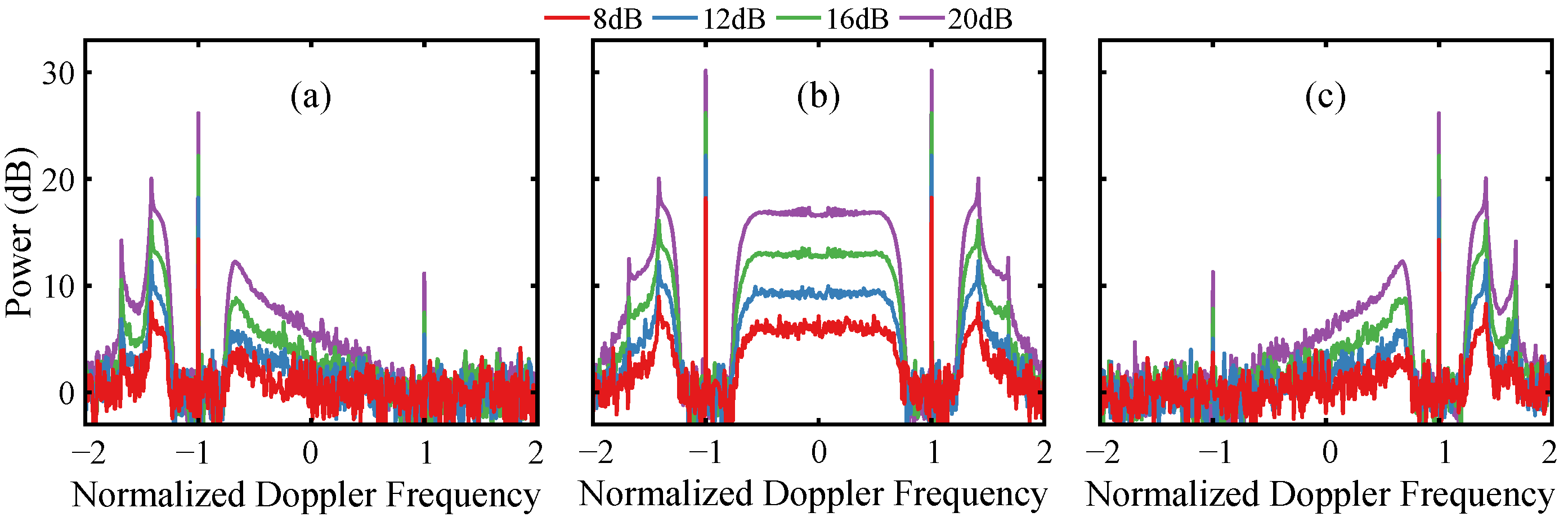
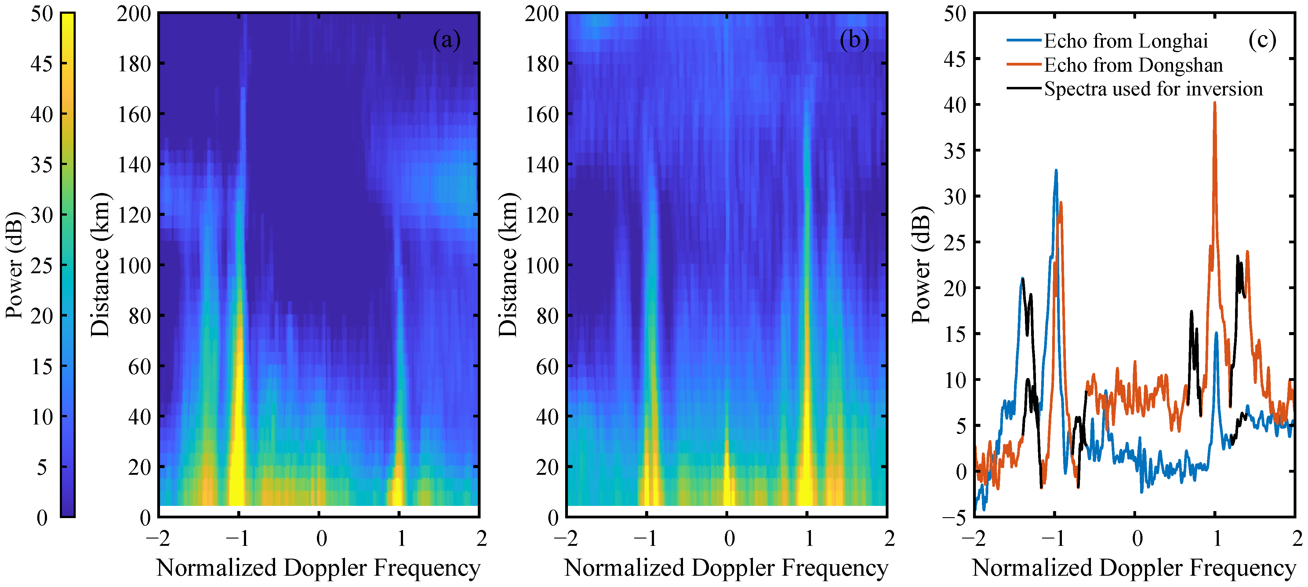
3.1. Radar Doppler Spectrum Simulation and Noise

According to the first- and second-order radar cross-section equations, the directional wave spectrum is required to simulate Doppler spectra, and it can be expressed as a product of the non-directional spectrum and the directional distribution. Usually, the PM spectrum and the Longuet-Higgins directional distribution model are most commonly used in theoretical simulations. It is vital to note that $S\left(k\right)$ in the Barrick equations is related to $S\left(f\right)$ in the PM spectrum by $S\left(k\right)=S\left(f\right){\displaystyle \frac{1}{k}}{\displaystyle \frac{df}{dk}}$.

The sea echoes received by radar systems are generally affected by various noise sources, so the simulated Doppler spectra need to be noised for approximation to reality. Because the Doppler spectrum is a PSD function, that of noise also needs to be estimated before being superimposed on the simulated spectrum. Thus, the total spectrum with noise is expressed as $P\left({\omega }_d\right)=P_s\left({\omega }_d\right)+P_n\left({\omega }_d\right)$, where $P_s\left({\omega }_d\right)$ is the simulated Doppler spectrum without noise and $P_n\left({\omega }_d\right)$ is the PSD of noise. In our simulations, as others usually do, the noise is assumed to be additive Gaussian white noise whose PSD is a constant.

The simulated Doppler spectra with several typical second-order peak SNRs are shown in Figure 6, where the simulation conditions include a radar operating frequency of 8 MHz, a radar beam directed to 0°, and a wind speed of 12 m/s. It can be seen that the Doppler spectra with weak energy are masked by noise as the peak SNRs decrease, resulting in a reduction in the second-order spectral points available for wave inversion.

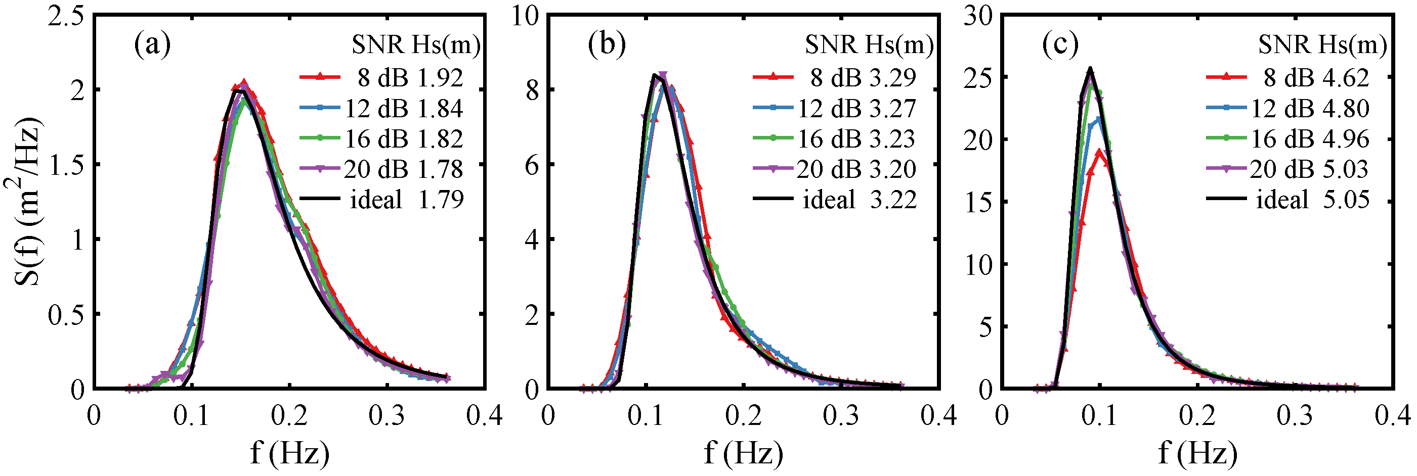
3.2. Single-Radar Inversion Simulation

In order to verify the effectiveness of the proposed inversion algorithm, a series of simulations in different scenarios are designed. By controlling the wind speed and wind direction, various theoretical wave spectra are generated, and then the corresponding Doppler spectra with noise are simulated for different second-order peak SNRs. The simulated Doppler spectra are used as input to the proposed algorithm to obtain inversion results which are compared with the ideal wave spectra for verification. Due to the random process involved, Monte Carlo experiments are performed in the simulations, and then the results are averaged for statistical analysis.

In the single-radar inversion simulation, the radar operating frequency is set to 8 MHz, the radar beam direction is 0°, and several typical conditions are considered, such as wind speeds of 9 m/s, 12 m/s, and 15 m/s; wind directions of 45°, 90°, and 135°; second-order peak SNRs of 8 dB, 12 dB, 16 dB, and 20 dB. The comparison of non-directional spectrum inversion results under low, medium, and high wind speeds is shown in Figure 7, and the comparison under several typical wind directions is shown in Figure 8. The inverted wave spectra are found to be in good agreement with the ideal curves, except for high wind speeds in the case of low SNRs, which is mainly due to the deviation of the optimal regularization parameter estimated by the empirical function.

Due to the directional ambiguity in the single-radar inversion, only the results of the non-directional spectrum are shown here. However, the angle $\theta$ between the wind direction and the radar beam has a certain degree of influence on the inversion accuracy of the non-directional spectrum. For example, we calculate the relative error, ${\displaystyle \frac{\Vert S_{\mathrm{inv}}\left(f\right)-S_{\mathrm{real}}{\left(f\right)\Vert }_2}{\Vert S_{\mathrm{real}}{\left(f\right)\Vert }_2}}$, where $S_{\mathrm{inv}}\left(f\right)$ is the inverted spectrum and $S_{\mathrm{real}}\left(f\right)$ is the real one, vs. $\theta$ for several wind speeds in the case of a second-order peak SNR of 16 dB, as shown in Figure 9. It is evident that the inverted non-directional spectra for the wind direction perpendicular to the radar beam are the most accurate, and the errors become larger with $\theta$ further away from 90°, which is mainly due to the reduction in the second-order spectral points available for wave inversion, while the fact that the response to waves propagating perpendicular to the radar is lower than that when they are propagating towards or away from the radar also affects the inversion accuracy.

To quantitatively evaluate the accuracy of the inverted wave spectra under different conditions, the significant wave height $H_s=4\sqrt{\int S\left(f\right)df}$ and the mean wave period $T_E={\displaystyle \frac{\int f^{-1}S\left(f\right)df}{\int S\left(f\right)df}}$ are calculated and compared with the theoretical values, and the absolute error statistics are shown in

Table 2. Error statistics of the wave parameters for single-radar inversion.

SNR (dB)		9 m/s			12 m/s			15 m/s
		${\mathbf{45}}^{\circ }$	${\mathbf{90}}^{\circ }$	${\mathbf{135}}^{\circ }$	${\mathbf{45}}^{\circ }$	${\mathbf{90}}^{\circ }$	${\mathbf{135}}^{\circ }$	${\mathbf{45}}^{\circ }$	${\mathbf{90}}^{\circ }$	${\mathbf{135}}^{\circ }$
8	$H_s$	0.18	0.13	0.15	0.12	0.07	0.13	0.52	0.43	0.46
	$T_E$	0.13	0.05	0.11	0.09	0.11	0.15	0.36	0.25	0.39
12	$H_s$	0.09	0.05	0.10	0.09	0.05	0.08	0.41	0.25	0.39
	$T_E$	0.08	0.06	0.12	0.16	0.10	0.15	0.23	0.13	0.27
16	$H_s$	0.08	0.03	0.09	0.07	0.01	0.05	0.24	0.09	0.36
	$T_E$	0.10	0.04	0.06	0.18	0.03	0.13	0.15	0.07	0.13
20	$H_s$	0.03	0.01	0.05	0.03	0.02	0.02	0.07	0.02	0.05
	$T_E$	0.05	0.03	0.03	0.06	0.02	0.07	0.05	0.02	0.09

For the two rows in the table body corresponding to an SNR, the first one represents the absolute error of the significant wave height in units of m, and the second one represents that of the mean wave period in units of s.

. As mentioned above, the absolute errors for high wind speeds in the case of low SNRs are relatively large. On the whole, the higher the SNR, the smaller the error in the results. However, some abnormal cases may occur due to the biased estimation of the optimal regularization parameter in some scenarios.

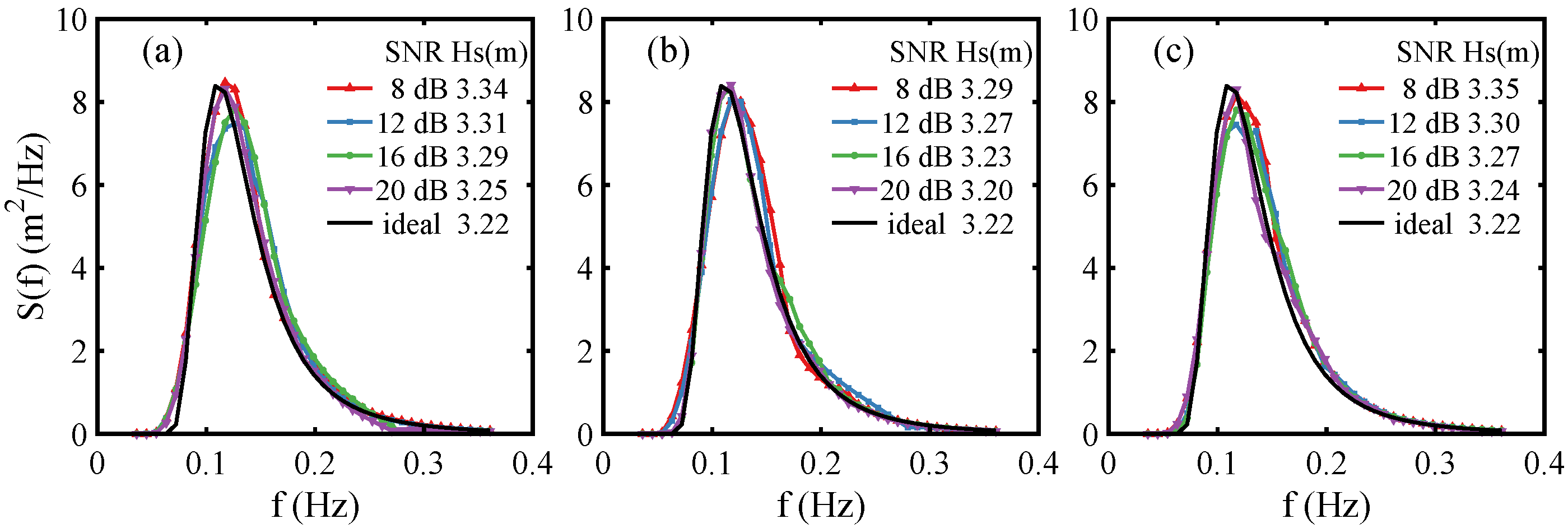
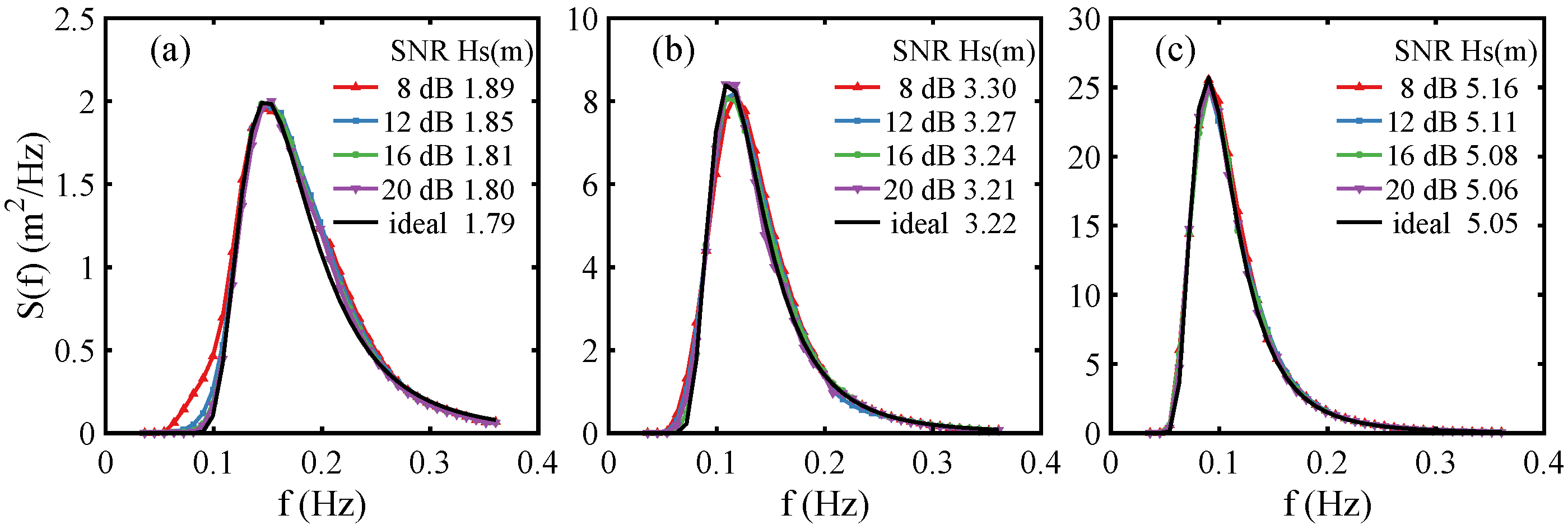
3.3. Dual-Radar Inversion Simulation

In the dual-radar inversion simulation, the beam direction of radar1 is set to −45°, and that of radar2 is set to 45°, while the other simulation conditions are the same as those in the single-radar inversion simulation. Although the angle between the beam directions of the two radars affects the inversion result, the statistical characteristics of inversion errors are not greatly different in the core detection area with an angle range of about 60°∼120°. The comparisons of non-directional spectrum inversion results under different wind speeds and wind directions are shown in Figure 10 and Figure 11, respectively, and the absolute error statistics are shown in

Table 3. Error statistics of the wave parameters for dual-radar inversion.

SNR (dB)		9 m/s			12 m/s			15 m/s
		${\mathbf{45}}^{\circ }$	${\mathbf{90}}^{\circ }$	${\mathbf{135}}^{\circ }$	${\mathbf{45}}^{\circ }$	${\mathbf{90}}^{\circ }$	${\mathbf{135}}^{\circ }$	${\mathbf{45}}^{\circ }$	${\mathbf{90}}^{\circ }$	${\mathbf{135}}^{\circ }$
8	$H_s$	0.13	0.10	0.11	0.09	0.08	0.07	0.15	0.11	0.12
	$T_E$	0.07	0.05	0.03	0.05	0.06	0.03	0.03	0.02	0.06
	${\theta }_m$	2.31	3.78	3.27	4.21	2.68	2.32	1.62	1.97	2.23
12	$H_s$	0.05	0.06	0.04	0.03	0.05	0.04	0.08	0.06	0.05
	$T_E$	0.02	0.03	0.05	0.03	0.03	0.02	0.02	0.01	0.04
	${\theta }_m$	1.45	2.13	1.77	1.18	1.89	1.22	1.10	0.85	1.26
16	$H_s$	0.01	0.02	0.02	0.01	0.02	0.02	0.01	0.03	0.02
	$T_E$	0.06	0.03	0.04	0.02	0.02	0.02	0.05	0.02	0.03
	${\theta }_m$	2.10	1.76	1.19	1.09	1.16	0.98	1.05	1.08	1.13
20	$H_s$	0.01	0.01	0.01	0.01	0.01	0.01	0.01	0.01	0.01
	$T_E$	0.02	0.02	0.03	0.01	0.02	0.01	0.03	0.01	0.02
	${\theta }_m$	0.86	1.55	1.12	1.21	0.73	0.87	1.13	0.52	0.96

For the three rows in the table body corresponding to an SNR, the first one represents the absolute error of the significant wave height in units of m, the second one represents that of the mean wave period in units of s, and the third one represents that of the mean wave direction in units of °.

. Because there is more observation information from different look directions, the estimated non-directional wave spectra are in better agreement with the theoretical curves for dual-radar systems than for single-radar systems, indicating that multiple-radar inversion is helpful in obtaining more accurate wave spectra.

The dual-radar systems observe the same sea surface patch from different directions, which can eliminate the directional ambiguity inherent in a single-radar system, and allow the directional wave spectrum to be obtained, then the directional distribution for waves at the peak frequency is calculated from the estimated directional wave spectrum. The comparisons of inversion results of the directional distribution under different wind speeds and wind directions are shown in Figure 12 and Figure 13, respectively, indicating that the extracted directional distributions and the theoretical curves are basically in agreement, except for low SNRs. The absolute error statistics of the mean wave direction ${\theta }_m={tan}^{-1}{\displaystyle \frac{\int \int S(f,\theta )sin\theta d\theta df}{\int \int S(f,\theta )cos\theta d\theta df}}$ under different conditions are also shown in Table 3, which shows that the mean wave direction errors are not more than 5° in the simulations, verifying the effectiveness of the proposed algorithm.

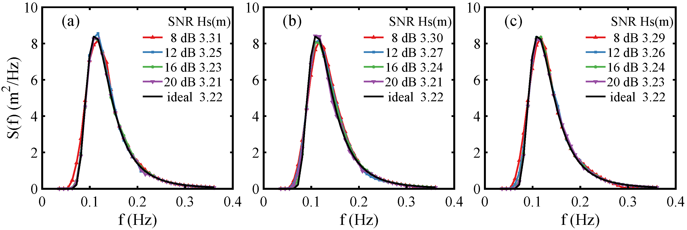
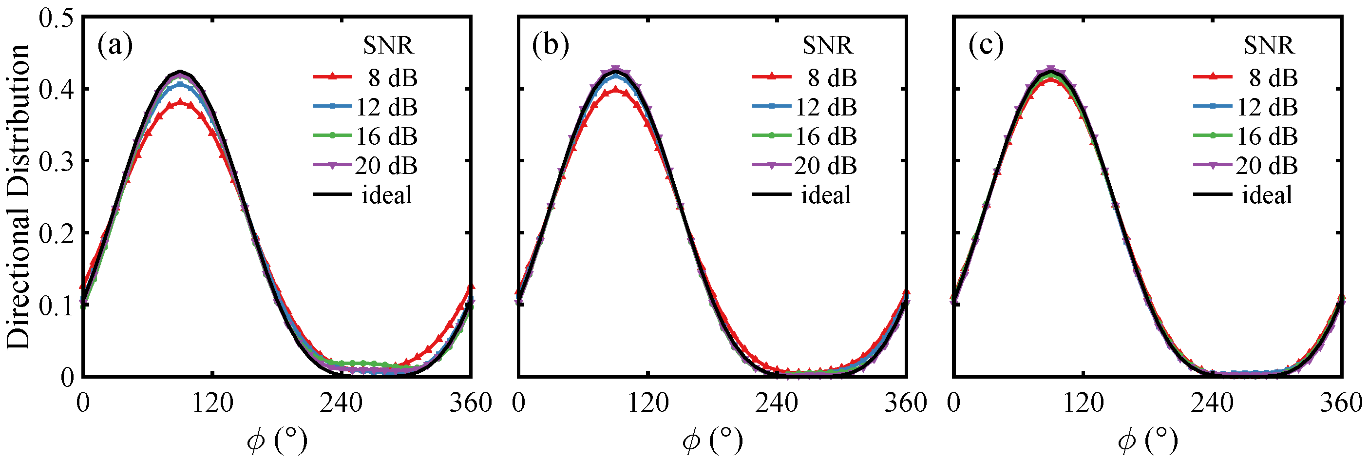
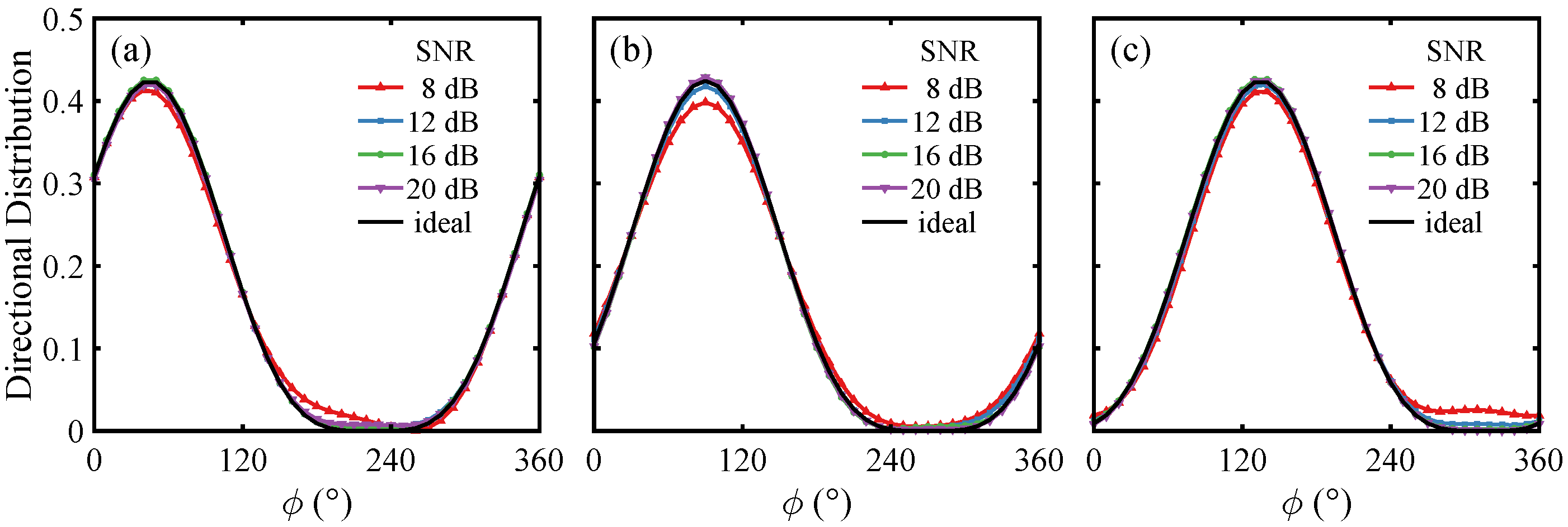
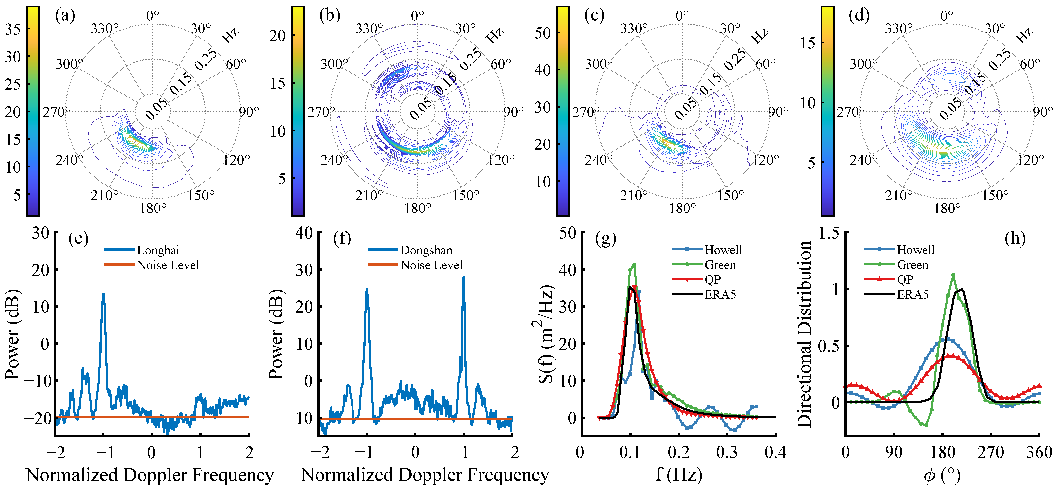
3.4. Directional Wave Spectrum Results

The buoy was returned to the port for repair after a long period of operation, resulting in a lack of availability of buoy data during this verification experiment. Fortunately, the European Center for Medium-Range Weather Forecasting (ECMWF) provides ERA5 reanalysis data for global atmospheric and oceanic parameters, which can be used to verify the wave results of this experiment. In this study, four typical locations in the common detection area are selected for comparison of the wave parameters, among which location P1 is about 70 km away from the two radar sites and location P2 is about 100 km away; location P3 is close to the shore and in shallow water, while location P4 is in deep water.

The RD spectra from Longhai and Dongshan in the direction of location P1 at 12:00 on 11 October 2021, are shown in Figure 14a and Figure 14b, respectively. At this moment, the first-order spectral peaks extend 180 km away, and the second-order spectral peaks extend up to 150 km. Since the direction of ocean waves is mainly along the Taiwan Strait from northeast to southwest during this period, the power of the negative Doppler spectral region is stronger than that of the positive spectral region for the Longhai site, while the opposite is true for the Dongshan site. The Doppler spectra from the two radar sites at location P1 are shown in Figure 14c. Since the inversion method proposed here is based on the linearization technique, only the second-order spectra near the first-order peaks should be selected for the wave inversion.

The inverted directional wave spectra at location P1 for several typical sea states during the verification experiment are compared with the ERA5 data, as shown in Figure 15. Overall, the spectral energy of the directional wave spectra from ERA5 and the dual-radar inversion is distributed basically in the same spectral region. However, the recorded wave spectra from ERA5 are more concentrated in direction, while the energy of the dual-radar inverted wave spectra is spread over a wider beamwidth, which can be seen evidently in the comparison of directional distributions shown in Figure 15a4,b4,c4. As mentioned in the methodology, the truncated second order of the Fourier series is chosen for the wave inversion, but it may not be sufficient in the case of very concentrated energy distributions in direction, which indicates that it is necessary for the processes in our inversion algorithm to be improved to support a larger truncated order, including the construction of constraints, the empirical criterion for estimating the optimal regularization parameter, the quadratic programming algorithm, and so on. In addition, the non-directional wave spectra from the dual-radar inversion that are less affected by the truncated order are more accurate than those from the single-radar inversion, which has also been verified in the simulations.

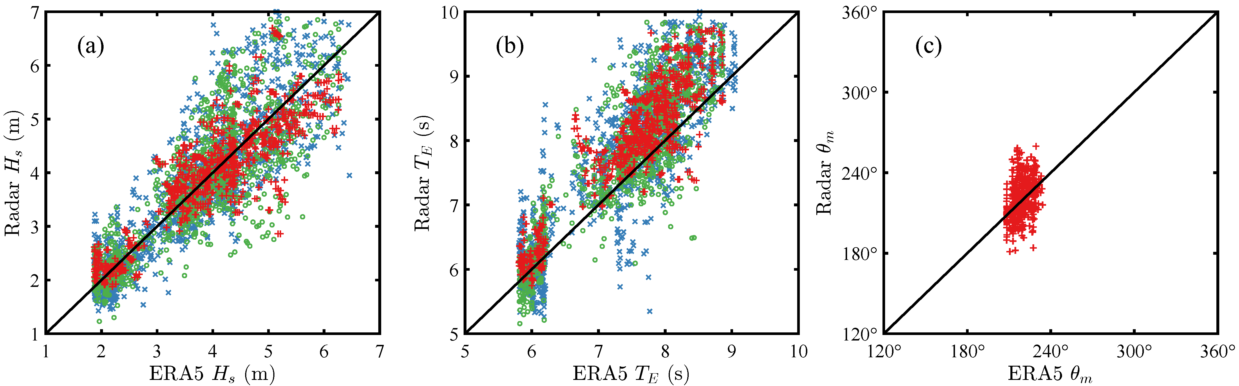
3.5. Wave Parameter Comparison

In order to further verify the performance of the proposed algorithm, wave parameters, including the significant wave height $H_s=4\sqrt{\int S\left(f\right)df}$, mean wave period $T_E={\displaystyle \frac{\int f^{-1}S\left(f\right)df}{\int S\left(f\right)df}}$, and mean wave direction ${\theta }_m={tan}^{-1}{\displaystyle \frac{\int \int S(f,\theta )sin\theta d\theta df}{\int \int S(f,\theta )cos\theta d\theta df}}$, are calculated from the measured directional wave spectra and compared with the ERA5 data. The comparison of these typical wave parameters at the four locations P1∼P4 is shown in Figure 16, and the second-order peak SNRs are also presented here. It can be seen that the SNRs have a certain daily periodicity, as they are usually high from 6 o’clock to 12 o’clock but very low from 18 o’clock to 24 o’clock. Generally, during the evening, the radio-frequency interference is serious, and the electromagnetic environment is more complex, which seriously affects the SNR of radar echoes from long distances. There is also a difference in the peak SNR of Doppler spectra from the two radar sites at the same time, so one of them may not participate in the wave inversion when its second-order peak SNR is lower than 6 dB. It can be seen in Figure 16 that all parameters have no output when both radar sites have a very low SNR, and only the single-radar results are outputted when the peak SNR of one site does not satisfy the requirement, while the dual-radar results are obtained only when the peak SNRs of both sites satisfy the requirement.

As shown in Figure 16, the significant wave height and mean wave period at each location, as well as the mean wave direction, are in reasonable agreement with the ERA5 data. However, there is a bias in the mean wave period between the ERA5 data and the radar results, which requires more measured data, such as that from a buoy, for further validation. The scatter diagram of these typical wave parameters is shown in Figure 17, where the consistency of each parameter can be seen more clearly. Then, the root mean square error (RMSE), correlation coefficient (CC), and number of samples for the statistics at the four locations are listed in

Table 4. Comparison of the wave parameters at each location.

Location	${\mathit{H}}_{\mathit{s}}$			${\mathit{T}}_{\mathit{E}}$			${\mathit{\theta }}_{\mathit{m}}$
	RMSE (m)	CC	No.	RMSE (s)	CC	No.	RMSE(°)	CC	No.
P1	0.60	0.88	382	0.62	0.87	382	-	-	-
	0.67	0.79	294	0.54	0.83	294	-	-	-
	0.46	0.90	258	0.52	0.89	258	10	0.24	258
P2	0.62	0.89	325	0.72	0.81	325	-	-	-
	0.87	0.79	171	0.69	0.86	171	-	-	-
	0.56	0.91	106	0.68	0.90	106	13	0.31	106
P3	0.67	0.86	328	0.78	0.92	328	-	-	-
	0.76	0.90	273	0.69	0.89	273	-	-	-
	0.63	0.89	197	0.72	0.91	197	15	0.15	197
P4	0.62	0.90	289	0.58	0.92	289	-	-	-
	0.65	0.86	280	0.66	0.92	280	-	-	-
	0.51	0.92	236	0.59	0.93	236	15	0.25	236

For the three rows in the table body corresponding to a location, the first one represents the results from the Longhai site, the second one represents those from the Dongshan site, and the third one represents those from the dual-radar inversion.

. For the single-radar results, the RMSE of the significant wave height is about 0.60∼0.87 m, and that of the mean wave period is about 0.54∼0.78 s, along with the CC of about 0.8∼0.9. For the dual-radar results, the RMSE of the significant wave height is about 0.46∼0.63 m, and that of the mean wave period is about 0.52∼0.72 s, along with the CC around 0.9. As for the mean wave direction, the RMSE is about 10∼15°, while its CC may not be useful due to the relatively small variation in direction during the experiment. In addition, the errors are relatively large at location P3 due to the shallow water.

The performance of the inversion algorithm is also evaluated with these wave parameters for several typical peak SNR levels.

Table 5. Comparison of the wave parameters for different second-order peak SNRs.

SNR (dB)	${\mathit{H}}_{\mathit{s}}$			${\mathit{T}}_{\mathit{E}}$			${\mathit{\theta }}_{\mathit{m}}$
	RMSE (m)	CC	No.	RMSE (s)	CC	No.	RMSE(°)	CC	No.
8	0.63	0.87	165	0.69	0.76	165	-	-	-
	0.75	0.84	223	0.62	0.88	223	-	-	-
	0.55	0.89	165	0.58	0.91	165	12	0.42	165
12	0.61	0.89	329	0.68	0.88	329	-	-	-
	0.68	0.86	284	0.72	0.85	284	-	-	-
	0.56	0.90	296	0.64	0.93	296	15	0.47	296
16	0.62	0.87	363	0.65	0.87	363	-	-	-
	0.59	0.83	266	0.68	0.86	266	-	-	-
	0.51	0.86	237	0.60	0.85	237	15	0.32	237
20	0.68	0.75	390	0.70	0.77	390	-	-	-
	0.75	0.69	209	0.66	0.83	209	-	-	-
	0.47	0.81	118	0.53	0.80	118	13	0.19	118

For the three rows in the table body corresponding to an SNR, the first one represents the results from the Longhai site, the second one represents those from the Dongshan site, and the third one represents those from the dual-radar inversion.

lists the results for the second-order peak SNRs of 8 dB, 12 dB, 16 dB, and 20 dB. Since the peak SNRs of Doppler spectra from the two radar sites are usually different at the same time, the smaller one is taken as the value for dual-radar statistics. If the value is less than 10 dB, this set of data is classified into the dataset of 8 dB; if the value is in the range of 10∼14 dB, this set of data is classified into the dataset of 12 dB; if the value is in the range of 14∼18 dB, this set of data is classified into the dataset of 16 dB; and if the value is greater than 18 dB, this set of data is classified into the dataset of 20 dB. For the single-radar results, the RMSE of the significant wave height is about 0.59∼0.75 m, and that of the mean wave period is about 0.62∼0.72 s, along with the CC of about 0.7∼0.9. For the dual-radar results, the RMSE of the significant wave height is about 0.47∼0.56 m, and that of the mean wave period is about 0.53∼0.64 s, along with the CC about 0.8∼0.9, while the RMSE of the mean wave direction is about 12∼15°. On the whole, as the peak SNR increases, the RMSE decreases, while some abnormal cases may occur due to many factors such as external interferences.

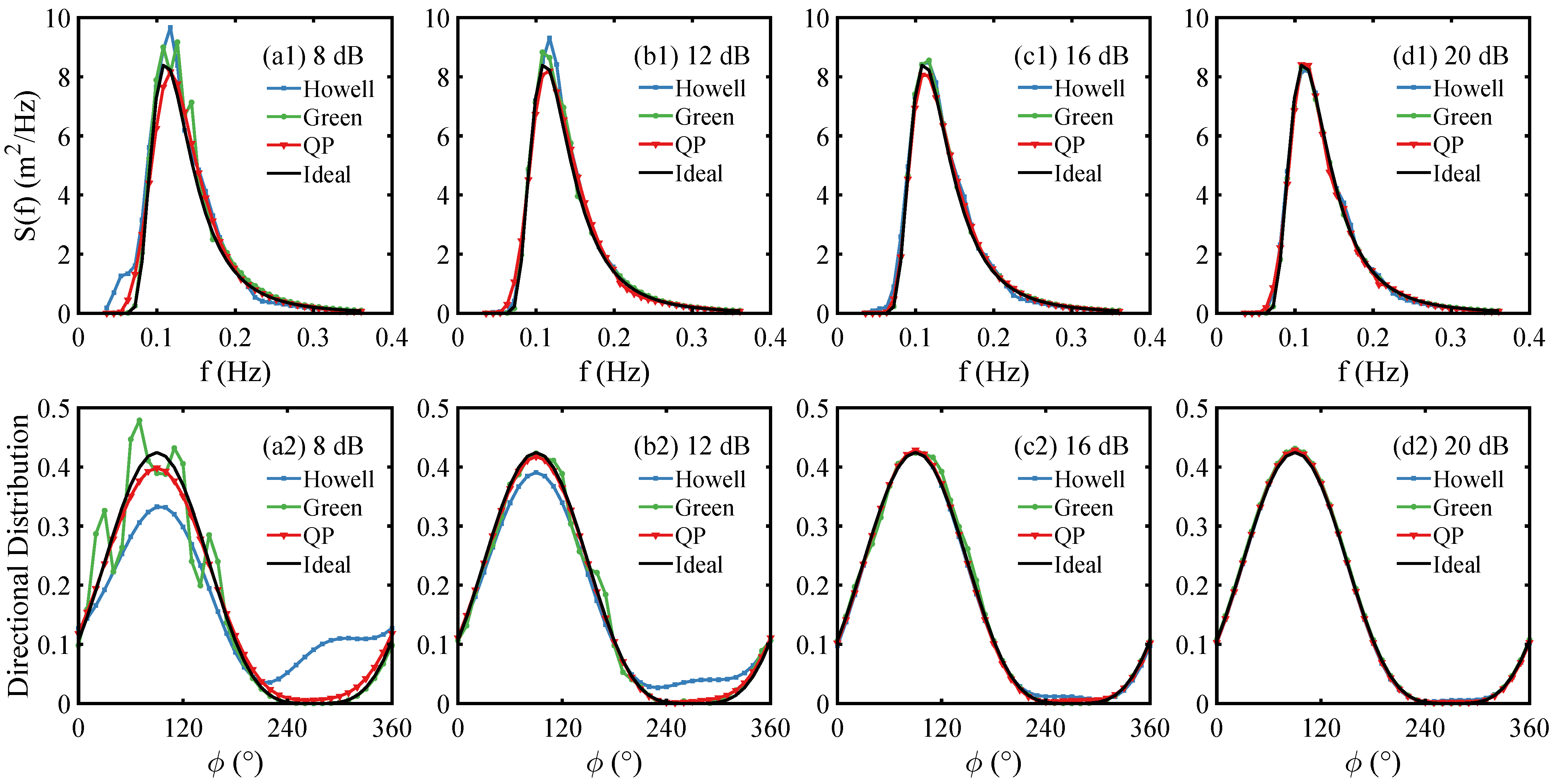
3.6. Method Comparison and Results

Here, we give some comparison results for testing against other methods to further verify the performance of the proposed method in low SNRs. Specifically, two methods that are widely used, i.e., the Howell method [12] and the Green method [24], are taken for comparison with our method (QP). The simulated Doppler spectra with different second-order peak SNRs are inverted using these methods to be compared with each other, where the wind speed and direction are 12 m/s and 90° and other conditions are the same as those mentioned above. Figure 18 shows the comparison of the non-directional wave spectrum in the single-radar inversion, and Figure 19 shows the comparison of the non-directional wave spectrum and directional distribution in the dual-radar inversion. For a quantitative comparison, the absolute errors of the wave parameters are calculated for each case, as listed in

Table 6. Absolute errors of the wave parameters for different second-order peak SNRs and methods.

SNR (dB)	Howell			Green			QP
	${\mathbf{H}}_{\mathbf{s}}$(m)	${\mathbf{T}}_{\mathbf{E}}$(s)	${\mathbf{\theta }}_{\mathbf{m}}$(°)	${\mathbf{H}}_{\mathbf{s}}$(m)	${\mathbf{T}}_{\mathbf{E}}$(s)	${\mathbf{\theta }}_{\mathbf{m}}$(°)	${\mathbf{H}}_{\mathbf{s}}$(m)	${\mathbf{T}}_{\mathbf{E}}$(s)	${\mathbf{\theta }}_{\mathbf{m}}$(°)
8	0.54	0.53	-	0.38	0.20	-	0.07	0.11	-
	0.27	0.42	9.60	0.19	0.04	5.64	0.08	0.06	2.68
12	0.32	0.37	-	0.17	0.06	-	0.05	0.10	-
	0.11	0.23	5.30	0.08	0.02	3.40	0.05	0.03	1.89
16	0.13	0.21	-	0.05	0.02	-	0.01	0.03	-
	0.08	0.15	1.54	0.05	0.03	2.37	0.02	0.02	1.16
20	0.05	0.12	-	0.03	0.03	-	0.02	0.02	-
	0.02	0.10	0.86	0.02	0.02	0.84	0.01	0.02	0.73

For the two rows in the table body corresponding to an SNR, the first one represents the results from the single-radar inversion, and the second one represents those from the dual-radar inversion.

. On the whole, these methods all work well in medium and high SNRs, while our method can obtain relatively accurate and stable inversion results in low SNRs.

Moreover, the measured Doppler spectra from Longhai and Dongshan are inverted for the method comparison, which were obtained at location P2 (about 100 km away from the two radar sites) at 10:00 on 11 October 2021. The second-order peak SNRs are about 12 dB and 9 dB for Longhai and Dongshan, respectively, as shown in Figure 20e,f. The inverted directional wave spectra from the Howell method, Green method, and our method (QP) are shown in Figure 20b,c,d, respectively, while Figure 20a shows that from ERA5. The comparisons of the non-directional spectrum and directional distribution are shown in Figure 20g and Figure 20h, respectively. For a quantitative comparison, the absolute errors of the wave parameters relative to the ERA5 data are 0.84 m, 23°, and 0.81 s for the Howell method; 0.66 m, 8°, and 0.62 s for the Green method; 0.54 m, 13°, and 0.57 s for our method. Overall, our method can obtain relatively accurate and stable inversion results in such a low SNR, while the directional distribution inverted by the Green method is in better agreement with that from the ERA5 data. In addition, the computational complexity is low for the Howell and Green methods, but our method takes about 20 s to complete one calculation due to the processes of quadratic programming and determination of the optimal regularization parameter.

4. Discussion

The directional wave spectra are estimated by the proposed method using the received echoes from the two radar sites, which are basically consistent with those from the ERA5 data. Further, the calculated wave parameters are seen to be in reasonable agreement with the ERA5 data at the four locations in the common detection area during the three-day experiment. Reasonable performance can also be obtained in the case of low SNRs, which preliminarily confirms the effectiveness of the wave inversion method proposed in this study. In the field experiment, the proposed algorithm is accurate in terms of the significant wave height and mean wave period, with an RMSE of up to 0.47 m and 0.53 s, respectively, and the CC can reach 0.9 or above. As for the mean wave direction, the RMSE is about 10°∼15°, while its CC may not have been a true reflection due to the relatively small variation in direction, which would require more datasets for validation. On the whole, the proposed algorithm performed reasonably in this experiment, which is helpful for improving the capacity of wave inversion in HFSWR.

There are still some problems to be solved. In some cases, a large bias is found between the estimated and true values of the optimal regularization parameter, leading to deviation of the inverted directional wave spectrum from the real one, which has been seen in the simulations and the field experiment. Although the optimal regularization parameter estimation criterion used in this study can be applied in most cases, further research on better criteria is recommended to address possible anomalies. In the field experiment, there is a limitation for the very concentrated directional distributions, which also requires improvement for the processes in our method to support a larger truncated order. The errors are also relatively large in shallow water because the algorithm in this study is mainly designed for deep-water cases. For solving this problem, the shallow-water wave model needs to be introduced into the inversion algorithm.

As for the fact that the performance of the proposed method in experiments is inferior to that in simulations, there are also some possible issues to be addressed. The additive Gaussian white noise is assumed in the simulations, which is convenient to generate and process. However, in field experiments, the statistical distribution of noise is very complex and may differ for various sea states, and there is also much interference from radio stations or the ionosphere, with both resulting in performance degradation to some extent. Although we have performed some averaging of the Doppler spectrum, the influence of different averaging schemes on wave measurements should be further investigated for our radar system. Secondly, our method is based on the linearized version of the integral equation, which has some limitations for high sea states where higher-order nonlinearities in the measured Doppler spectra may occur [39]. In addition, the ERA5 data are calculated with numerical ocean wave models, which may be different from the true values to some extent. If conditions permit, a wave buoy should be deployed to obtain more accurate wave information on these Fourier coefficients for comparison.

5. Conclusions

In this study, a quadratic programming method based on the regularization technique is proposed to estimate the directional wave spectrum, and an empirical criterion for estimating the optimal regularization parameter is given. The effectiveness of the inversion algorithm is preliminarily tested using simulated Doppler spectra under different wind speeds and wind directions, while Gaussian white noise is considered in the simulations. The inversion results are found to be in good agreement with the theoretical ones for the radar operating frequency of 8 MHz. Further, a three-day radar dataset was collected during a storm, when the significant wave height increased from 2 m to about 6 m and then returned to 2 m. Due to the lack of buoy data in this experiment, the ERA5 reanalysis data was used for comparison to verify the performance of the algorithm. The radar inverted directional wave spectra are basically consistent with those from the ERA5 data, while there is a limitation for the very concentrated directional distributions due to the truncated second order in the Fourier series. In addition, the typical wave parameters are calculated from the estimated directional wave spectra to be compared with the ERA5 data, and the results show that the inversion algorithm has reasonable performance for different second-order peak SNRs in the core detection area.

However, the algorithm does not obtain the optimal regularization parameter in some cases, and the performance may worsen in high sea states or in shallow water. In future research, it is recommended to optimize the optimal regularization parameter estimation criterion to improve the inversion algorithm. The dataset used has little variation in spectral shape apart from the changes in amplitude and peak frequency during the storm. Thus, verification with a longer dataset (preferably from a buoy) that includes a much wider range of wave conditions is required for a comprehensive evaluation of the method. In addition, the simulations and experiments were carried out at the radar operating frequency of 8 MHz, but the performance of the algorithm could be verified using other operating frequencies, while the multi-frequency fusion scheme is also expected to further reduce the inversion errors of the directional wave spectrum.

References

1. Crombie, D.D. Doppler spectrum of sea echo at 13.56 Mc./s. Nature 1955, 175, 681–682. [Google Scholar] [CrossRef]
2. Barrick, D.E. Remote sensing of sea state by radar. In Proceedings of the Ocean 72—IEEE International Conference on Engineering in the Ocean Environment, Newport, RI, USA, 13–15 September 1972; pp. 186–192. [Google Scholar]
3. Gurgel, K.W.; Antonischki, G.; Essen, H.H.; Schlick, T. Wellen radar (WERA): A new ground-wave HF radar for ocean remote sensing. Coast. Eng. 1999, 37, 219–234. [Google Scholar] [CrossRef]
4. Barrick, D.E.; Weber, B.L. On the nonlinear theory for gravity waves on the ocean’s surface. Part II: Interpretation and applications. J. Phys. Oceanogr. 1977, 7, 11–21. [Google Scholar] [CrossRef]
5. Fujii, S.; Heron, M.L.; Kim, K.; Lai, J.W.; Lee, S.H.; Wu, X.; Wu, X.; Wyatt, L.R.; Yang, W.c. An overview of developments and applications of oceanographic radar networks in Asia and Oceania countries. Ocean Sci. J. 2013, 48, 69–97. [Google Scholar] [CrossRef]
6. Barrick, D.E. The ocean waveheight nondirectional spectrum from inversion of the HF sea-echo Doppler spectrum. Remote Sens. Environ. 1977, 6, 201–227. [Google Scholar] [CrossRef]
7. Lipa, B. Derivation of directional ocean-wave spectra by integral inversion of second-order radar echoes. Radio Sci. 1977, 12, 425–434. [Google Scholar] [CrossRef]
8. Lipa, B. Inversion of second-order radar echoes from the Sea. J. Geophys. Res.-Oceans 1978, 83, 959–962. [Google Scholar] [CrossRef]
9. Wyatt, L.R. The measurement of the ocean wave directional spectrum from HF radar Doppler spectra. Radio Sci. 1986, 21, 473–485. [Google Scholar] [CrossRef]
10. Wyatt, L.R. A relaxation method for integral inversion applied to HF radar measurement of the ocean wave directional spectrum. Int. J. Remote Sens. 1990, 11, 1481–1494. [Google Scholar] [CrossRef]
11. Gill, E.W.; Walsh, J. Extraction of ocean wave parameters from HF backscatter received by a four-element array: Analysis and application. IEEE J. Ocean. Eng. 1992, 17, 376–386. [Google Scholar] [CrossRef]
12. Howell, R.; Walsh, J. Measurement of ocean wave spectra using narrow-beam HF radar. IEEE J. Ocean. Eng. 1993, 18, 296–305. [Google Scholar] [CrossRef]
13. Hisaki, Y. Nonlinear inversion of the integral equation to estimate ocean wave spectra from HF radar. Radio Sci. 1996, 31, 25–39. [Google Scholar] [CrossRef]
14. Li, L.; Wu, X.; Long, C.; Liu, B. Regularization inversion method for extracting ocean wave spectra from HFSWR sea echo. Chinese J. Geophys. 2013, 56, 219–229. [Google Scholar]
15. Hisaki, Y. Ocean wave parameters and spectrum estimated from single and dual high-frequency radar systems. Ocean Dyn. 2016, 66, 1065–1085. [Google Scholar] [CrossRef]
16. Lopez, G.; Conley, D.C.; Greaves, D. Calibration, validation, and analysis of an empirical algorithm for the retrieval of wave spectra from HF radar sea echo. J. Atmos. Ocean. Technol. 2016, 33, 245–261. [Google Scholar] [CrossRef]
17. Lopez, G.; Conley, D.C. Comparison of HF radar fields of directional wave spectra against in situ measurements at multiple locations. J. Mar. Sci. Eng. 2019, 7, 271. [Google Scholar] [CrossRef]
18. Silva, M.T.; Shahidi, R.; Gill, E.W.; Huang, W. Nonlinear extraction of directional ocean wave spectrum from synthetic bistatic high-frequency surface wave radar data. IEEE J. Ocean. Eng. 2020, 45, 1004–1021. [Google Scholar] [CrossRef]
19. Shahidi, R.; Gill, E.W. A new automatic nonlinear optimization-based method for directional ocean wave spectrum extraction from monostatic HF-radar data. IEEE J. Ocean. Eng. 2021, 46, 900–918. [Google Scholar] [CrossRef]
20. Zhao, C.; Deng, M.; Chen, Z.; Ding, F.; Huang, W. Ocean wave parameters and nondirectional spectrum measurements using multifrequency HF radar. IEEE Trans. Geosci. Remote Sens. 2022, 60, 1–13. [Google Scholar] [CrossRef]
21. Wyatt, L.R.; Green, J.J. Developments in scope and availability of HF radar wave measurements and robust evaluation of their accuracy. Remote Sens. 2023, 15, 5536. [Google Scholar] [CrossRef]
22. Hardman, R.L.; Wyatt, L.R. Inversion of HF radar Doppler spectra using a neural network. J. Mar. Sci. Eng. 2019, 7, 255–272. [Google Scholar] [CrossRef]
23. Lewitt, R.M. Multidimensional digital image representations using generalized Kaiser–Bessel window functions. J. Opt. Soc. Am. A 1990, 7, 1834–1846. [Google Scholar] [CrossRef] [PubMed]
24. Green, J.J.; Wyatt, L.R. Row-action inversion of the Barrick-Weber equations. J. Atmos. Ocean. Technol. 2006, 23, 501–510. [Google Scholar] [CrossRef]
25. Longuet-Higgins, M.S.; Cartwright, D.E.; Smith, N.D. Observation of the directional spectrum of sea waves using the motions of a floating buoy. In Proceedings of the Ocean Wave Spectra, Easton, MD, USA, 1–4 May 1963; pp. 111–132. [Google Scholar]
26. Xie, X.; Zhang, L.; Chen, Z.; Wu, X.; Yue, X. MIMO ground wave radar radio frequency monitoring. IEEE Geosci. Remote Sens. Lett. 2022, 19, 1–5. [Google Scholar] [CrossRef]
27. Wang, M.; Wu, X.; Zhang, L.; Yue, X.; Yi, X.; Xie, X.; Yu, L. Measurement and analysis of antenna pattern for MIMO HF surface wave radar. IEEE Antennas Wirel. Propag. Lett. 2023, 22, 1788–1792. [Google Scholar] [CrossRef]
28. Bliss, D.W.; Forsythe, K.W. Multiple-input multiple-output (MIMO) radar and imaging: Degrees of freedom and resolution. In Proceedings of the Thrity-Seventh Asilomar Conference on Signals, Systems & Computers, 2003, Pacific Grove, CA, USA, 9–12 November 2003; Volume 1, pp. 54–59. [Google Scholar]
29. Lesturgie, M. Improvement of high-frequency surface waves radar performances by use of multiple-input multiple-output configurations. IET Radar Sonar Navig. 2009, 3, 49–61. [Google Scholar] [CrossRef]
30. Barrick, D.E.; Snider, J.B. The statistics of HF sea-echo Doppler spectra. IEEE Trans. Antennas Propag. 1977, 25, 19–28. [Google Scholar] [CrossRef]
31. Wyatt, L.R.; Green, J.J.; Middleditch, A. Signal sampling impacts on HF radar wave measurement. J. Atmos. Ocean. Technol. 2009, 26, 793–805. [Google Scholar] [CrossRef]
32. Barrick, D.E. First-order theory and analysis of MF/HF/VHF scatter from the sea. IEEE Trans. Antennas Propag. 1972, 20, 2–10. [Google Scholar] [CrossRef]
33. Rice, S.O. Reflection of electromagnetic waves from slightly rough surfaces. Commun. Pure Appl. Math. 1951, 4, 351–378. [Google Scholar] [CrossRef]
34. Barrick, D.E.; Lipa, B.J. The second-order shallow-water hydrodynamic coupling coefficient in interpretation of HF radar sea echo. IEEE J. Ocean. Eng. 1986, 11, 310–315. [Google Scholar] [CrossRef]
35. Howell, R.K. An Algorithm for the Extraction of Ocean Wave Spectra from Narrow Beam HF Radar Backscatter. Master’s Thesis, Memorial University of Newfoundland, St. John’s, NF, Canada, 1990. [Google Scholar]
36. Hasselmann, K. Determination of ocean wave spectra from Doppler radio return from the sea surface. Nature Phys. Sci. 1971, 229, 16–17. [Google Scholar] [CrossRef]
37. Phillips, O.M. The Dynamics of the Upper Ocean; Cambridge University Press: London, UK, 1966. [Google Scholar]
38. Moskowitz, L. Estimates of the power spectrums for fully developed seas for wind speeds of 20 to 40 knots. J. Geophys. Res. 1964, 69, 5161–5179. [Google Scholar] [CrossRef]
39. Wyatt, L.R. High order nonlinearities in HF radar backscatter from the ocean surface. IEE Proc.-Radar Sonar Navig. 1995, 142, 293–300. [Google Scholar] [CrossRef]
Figure 1. The diagram of the system model.
Remotesensing 17 02573 g001
Figure 2. Geographical map of the field experiment. The red ★ indicates the two radar sites located in Longhai and Dongshan. The sectors enclosed by the yellow lines indicate the core detection area of the two radar sites. There are four locations in the common detection area for comparison of the wave parameters, namely, P1 marked with +, P2 marked with ∘, P3 marked with ×, and P4 marked with □.
Remotesensing 17 02573 g002
Figure 3. The relative error vs. D for different second-order peak SNRs.
Remotesensing 17 02573 g003
Figure 4. Schematic diagram of estimating the optimal regularization parameter.
Remotesensing 17 02573 g004
Figure 5. Directional wave spectrum inversion flowchart.
Remotesensing 17 02573 g005
Figure 6. Simulated Doppler spectra with different second-order peak SNRs: (a) wind direction 45°; (b) wind direction 90°; (c) wind direction 135°.
Remotesensing 17 02573 g006
Figure 7. Comparison of the single-radar non-directional spectrum for different wind speeds when the wind direction is 90°: (a) wind speed 9 m/s; (b) wind speed 12 m/s; (c) wind speed 15 m/s.
Remotesensing 17 02573 g007
Figure 8. Comparison of the single-radar non-directional spectrum for different wind directions when the wind speed is 12 m/s: (a) wind direction 45°; (b) wind direction 90°; (c) wind direction 135°.
Remotesensing 17 02573 g008
Figure 9. Inversion accuracy of the non-directional spectrum vs. the angle θ .
Remotesensing 17 02573 g009
Figure 10. Comparison of the dual-radar non-directional spectrum for different wind speeds when the wind direction is 90°: (a) wind speed 9 m/s; (b) wind speed 12 m/s; (c) wind speed 15 m/s.
Remotesensing 17 02573 g010
Figure 11. Comparison of the dual-radar non-directional spectrum for different wind directions when the wind speed is 12 m/s: (a) wind direction 45°; (b) wind direction 90°; (c) wind direction 135°.
Remotesensing 17 02573 g011
Figure 12. Comparison of the directional distribution for different wind speeds when the wind direction is 90°: (a) wind speed 9 m/s; (b) wind speed 12 m/s; (c) wind speed 15 m/s.
Remotesensing 17 02573 g012
Figure 13. Comparison of the directional distribution for different wind directions when the wind speed is 12 m/s: (a) wind direction 45°; (b) wind direction 90°; (c) wind direction 135°.
Remotesensing 17 02573 g013
Figure 14. Doppler spectra at 12:00 on 11 October 2021. (a) RD spectrum from Longhai in the direction of location P1. (b) RD spectrum from Dongshan in the direction of location P1. (c) Doppler spectra from the two radar sites at location P1, where the black solid lines represent the second-order spectra used for the wave inversion.
Remotesensing 17 02573 g014
Figure 15. Comparison of the directional wave spectra at location P1 for several typical sea states during the verification experiment. (a1,a2) show the directional wave spectra from ERA5 and the dual-radar inversion, respectively, at 09:00 on 10 October 2021, when H s was about 2 m, while (a3,a4) show the comparison of the non-directional spectrum and the directional distribution, respectively. Similarly, (b1b4) and (c1c4) show the results at 15:00 on 11 October 2021, when H s was about 5.5 m, and at 15:00 on 12 October 2021, when H s was about 3.5 m, respectively. The contour map of the directional wave spectrum is drawn in polar coordinates referenced to true north. The color bar to the left of each contour map represents the spectral density of the directional wave spectrum in m 2 s / rad .
Remotesensing 17 02573 g015
Figure 16. Comparison of the typical wave parameters. (a1a4) show the comparison of the significant wave height at locations P1∼P4, respectively, (b1b4) show the comparison of the mean wave period, and (c1c4) show the comparison of the mean wave direction. Meanwhile, (d1d4) show the second-order peak SNRs. The black solid lines represent ERA5 data, and the red + represents the dual-radar measurements, while the blue × and green ∘ represent the single-radar results from Longhai and Dongshan, respectively.
Remotesensing 17 02573 g016
Figure 17. Scatter diagram of the typical wave parameters: (a) significant wave height; (b) mean wave period; (c) mean wave direction. The red + represents the dual-radar measurements, while the blue × and green ∘ represent the single-radar results from Longhai and Dongshan, respectively.
Remotesensing 17 02573 g017
Figure 18. Method comparison of the single-radar inversion for different second-order peak SNRs.
Remotesensing 17 02573 g018
Figure 19. Method comparison of the dual-radar inversion for different second-order peak SNRs.
Remotesensing 17 02573 g019
Figure 20. Method comparison using the measured Doppler spectra. (ad) show the directional wave spectra of ERA5, Howell, Green, and QP, respectively. (e,f) show the measured Doppler spectra from Longhai and Dongshan, respectively. (g) shows the comparison of the non-directional spectrum of each method, and (h) shows the comparison of the directional distribution. The color bar to the left of each contour map represents the spectral density of the directional wave spectrum in m 2 s / rad .
Remotesensing 17 02573 g020