Increasing the Thematic Resolution for Trees and Built Area in a Global Land Cover Dataset Using Class Probabilities

Abstract

Land cover-based models that rely on purpose-specific thematic details are common in environmental fields such as hydrology, water quality, and ecology. Global remotely sensed land cover from the Dynamic World dataset on Google Earth Engine has trees and built area classes, but enables modelers to create more thematically detailed classifications based on pixel class probabilities from their convolutional neural network (CNN) classifier. However, more information is needed about how these probabilities relate to actual heterogeneity within a land cover class. We used Dynamic World CNN class probabilities to subclassify temperate and tropical forest types from the trees class in the Eastern United States and Costa Rica, as well as developed area intensities from the built class. Subclassifications were evaluated against reference data and in a watershed they were not trained for. The results on dominant temperate forest type user’s accuracy (i.e., of all the pixels classified as a specific land cover type, how many are actually that type) ranged from 43% to 76%, while producer’s accuracy (i.e., of all the actual pixels of a specific land cover type, how many were correctly classified) ranged from 50% to 70%. In the untrained watershed, the overall accuracy was 85% for temperate forest types and 52% for developed areas, demonstrating reliability in classifying forest and developed land cover types. This approach creates opportunities to access up-to-date land cover information with greater thematic detail.

1. Introduction

Environmental models based on land cover data are common in many fields including hydrology, ecology, and freshwater science [1,2,3,4,5]. Often, these models are based upon the frameworks of readily available remotely sensed land cover datasets. For example, the Soil and Water Assessment Tool (SWAT [6]) and Generalized Watershed Loading Functions (GWLF [7]) models, used in thousands of water quality and hydrologic investigations, commonly input detailed classifications of the United States National Land Cover Database (NLCD [8]) and Cropland Data Layer [9]. However, these thematically detailed land cover products are often restricted to the USA, Europe, and other data-privileged regions, creating an inequity in regions that do not have these datasets readily available. Although global land cover products are available [10,11], they are typically of coarse thematic resolution, such as the ESA WorldCover 2020 and 2021 datasets which have 11 discrete classes to represent the Earth’s terrestrial surface and do not distinguish types of forest or intensities of developed land [12,13].

A lack of information about how land use and land use change affect hydrologic and water quality processes can impede freshwater policy and management decisions in data-scarce regions such as the tropics, including decisions for land use planning, biodiversity conservation, water resource availability assessment, and valuing ecosystem services [14,15,16,17]. There can be difficulties when land cover-based models are applied to other regions of the globe not covered by a specific land cover classification scheme, if more current land cover conditions are desired than the typical (e.g., 1–5 year) data releases, if extensive resources are not available for classifications [18,19], or if finer resolution and more thematic information is desired [20]. These difficulties could be addressed by improving equity in access to custom-classified, analysis-ready land cover information [21,22].

Near real-time remotely sensed land cover available in the Dynamic World dataset (from Google, the World Resources Institute, and National Geographic) creates the opportunity for modelers to customize land cover data for modeling cases around the globe by providing data about pixel class probabilities [23,24]. Pixel class probabilities are information about confidences of the Dynamic World convolutional neural network (CNN) algorithm in classifying land cover into nine discrete classes, and are available as vectors of percents for each class for every pixel [25,26]. For example, in addition to a land cover pixel being classified as “built” (i.e., urban), pixel class probabilities provide more details about the land cover dynamics (e.g., 70% probability for built, 20% for trees, and 10% for other types), based on the interpretations of the CNN used to classify the data. Pixel class probabilities can be an effective tool in distinguishing land cover types because they exhibit spatial and temporal autocorrelation over a time series of images, enabling the classification of pixels into discrete classes [27,28]. Thus, information about pixel class probabilities could potentially be used to subclassify land cover beyond the nine traditional Dynamic World classes (built, trees, etc.), into customizable classifications tailored to specific modeling purposes [24,29,30].

However, for the Earth and environmental sciences to take advantage of the benefits from a class probability subclassification approach, a better understanding is needed of the extent to which the class probabilities relate to traditional modeling approaches and real-world heterogeneities. The class probability subclassification approach involves several relevant knowledge gaps. First, confusion between land cover types can cause difficulties in understanding land cover heterogeneities and relating class probabilities with land cover transitions, particularly when comparing data with different spatial resolutions [31] or investigating causes of land cover change [32]. Second, edges between land cover types can be difficult to create temporally stable classifications for, especially concerning the influence of vegetation phenology in sub-annual classifications [33]. Finally, the high-resolution Dynamic World product is used for land cover studies around the globe (e.g., [34,35]), but there is a need for evaluating its class probabilities outputs with regard to land cover heterogeneities and gradients, which could provide crucial information about the thematic benefits of using class probabilities for a wide variety of land cover product users internationally [29].

To help address these knowledge gaps, we evaluated the use of CNN-based class probabilities from the Dynamic World dataset to increase the thematic resolution of land cover in four cases of protected areas in the eastern United States and Costa Rica. In each case, we compared the class probability approach with existing land cover data for validation. We asked, “To what extent can remotely sensed land cover pixel class probabilities from a global dataset be used to increase thematic resolution for trees and built area?” To help answer this question, we also analyzed the approach in comparison to potential seasonal variation and a human-referenced dataset. Our evaluation of this approach provides information about how much the pixel class probabilities could improve access to more thematically detailed land cover information, which could be of interest for environmental studies around the globe.

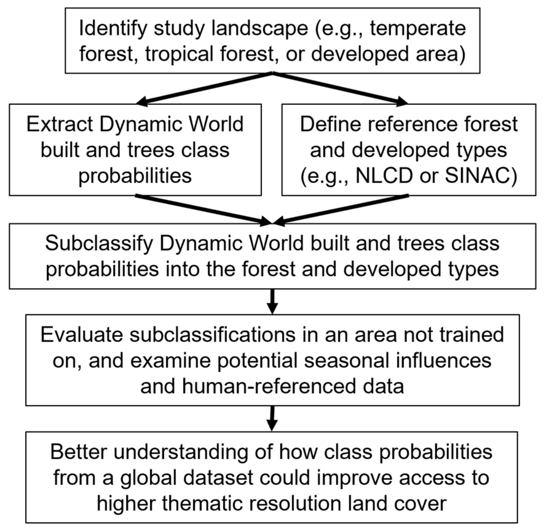
2. Materials and Methods

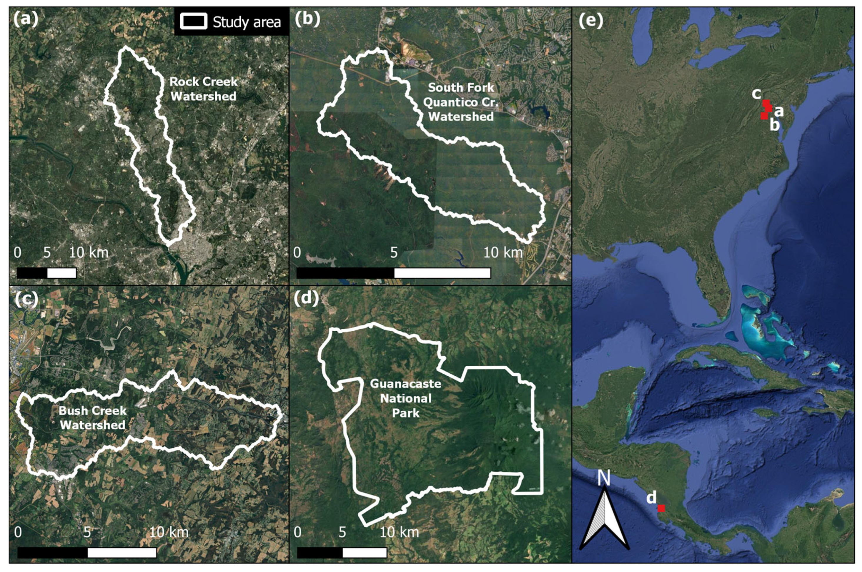
2.1. Site Design

Our study area consisted of four experimental landscapes that represent diverse forest types and developed intensities and complement existing freshwater management initiatives. The first three are temperate watersheds in the eastern United States that were identified as important to management of National Parks. The Rock Creek Watershed is dominated by developed land cover of various intensities from open space to high-intensity developed areas, as well as flowing through the forested Rock Creek Park (Figure 1a). The South Fork Quantico Creek watershed is dominated by temperate forest including deciduous, evergreen, and mixed stands (Figure 1b). The Bush Creek watershed has a mixture of temperate forest, agricultural, and developed lands (Figure 1c). Approximately 95% of the South Fork Quantico Creek watershed is considered protected land (all types including National Parks) and 22% of the Rock Creek Watershed is protected land, while only 6% of the Bush Creek watershed is protected [36]. The fourth experimental landscape is at the Guanacaste National Park, Costa Rica, where the Stroud Water Research Center operates the Maritza Biological Station to study tropical freshwater management (Figure 1d,e).

2.2. Land Cover Data

We used Google Earth Engine to extract Dynamic World 2022 data for the study watersheds (

Table 1. Descriptions of the land cover datasets used in this study.

Dataset	Spatial Resolution	Temporal Resolution	Classes Used	Span Used	Source
Dynamic World	10 m	~5 day	Built, trees	2015–2023	[23]
National Land Cover Database (NLCD)	30 m	Annual or longer	Open space, low intensity, medium, intensity, and high-intensity developed; deciduous, evergreen, and mixed forest	2019	[8]
Costa Rica National System of Conservation Areas (SINAC)	5 m	Annual or longer	Deciduous, secondary, and mature forest	2019	[39]
Dynamic World training dataset	10 m	Image	Built, trees	2019	[40]

). The data consisted of a series of land cover images collected at approximately 5-day intervals throughout the year from 1 January 2022 to 31 December 2022. This is a subset of the entire global Dynamic World dataset, which runs from 2015 to near real-time. From these data, we generated the dominant (mode statistic) land cover class over the year, as well as the mean pixel class probability of each class over the year. A diagram of the pixel class probability approach and spatiotemporal variability is presented in Figure 2a–e. Lower pixel class probabilities for edges between land cover types (e.g., where a built area meets a forest; Figure 2a,d) are more difficult to classify, which explains why their probabilities can be lower than pixels well within a homogenous land cover parcel (Figure 2c,e) [38]. Dynamic World data have a comparable accuracy to other remotely sensed global land cover products developed from Sentinel-2 images [24]. Spatial tropical forest data were obtained from the Costa Rica National System of Conservation Areas (SINAC) from 2019 including deciduous, secondary, and mature forest [39]. NLCD data for evaluations were obtained for the year 2019.

Although we used the Dynamic World dataset and thus did not train and use a new CNN in this study, we provide for background the process of convolution and classification in Supplementary Figure S1. The effectiveness of CNNs in land classification is underscored by their superior performance compared to traditional machine learning methods. For instance, CNNs can classify very high-resolution remote sensing images with remarkable accuracy, highlighting their utility in crop classification and scene-based classification tasks [41]. Similarly, Zhang et al. [42] emphasize the powerful feature extraction capabilities of CNNs, which allow for the identification of abstract and invariant features in remote sensing images, thereby enhancing classification performance. Further details about the Dynamic World CNN model, architecture, and data preprocessing can be found in [23], the model code is available from [43], and the dataset used to train the model can be found at [40]. In summary, the Dynamic World model used Sentinel-2 Level-2A calibrated surface reflectance to train the classifier and Sentinel-2 Level 1C top-of-atmosphere data to create the land cover dataset [23]. Data preprocessing for the Dynamic World model included masking clouds and shadows using Sentinel-2 Cloud Probability and cirrus band data and the Cloud Displacement Index (CDI) algorithm [23,44,45]. The architecture of the Dynamic World model was is a fully convolutional neural network which efficiently converts Sentinel-2 bands into class probabilities for nine land cover types [23,46].

2.3. Subclassification

2.3.1. Probability Thresholds

To distinguish subclasses from Dynamic World data, we applied custom probability thresholds as introduced in [24]. We chose these thresholds by evaluating against the NLCD and SINAC reference using a comparison of proportions of total land area, by calculating overall, producer’s, and user’s accuracy [47,48] (Equations (1)–(4)), and by visually verifying against Google and ESRI satellite imagery basemaps in each experiment (Figure 3). Comparisons of total land area were pertinent because models using land cover data, such as for hydrology and water quality, frequently use this statistic in their calculations, for instance the proportion of watershed subbasin that is developed or forested [3,6]. We replicated the evaluations with a small number of probability thresholds (0.66, 0.67, 0.68, etc.) for each class until the most suitable was chosen, beginning with the subclass with the highest pixel class probabilities, so that the pixels with the highest confidence of belonging to the discrete Dynamic World class would be extracted before those with lower confidence. Thus, high-intensity developed, evergreen forest, and mature forest would be extracted from the class probability data, followed by the subclasses with the next highest probabilities (medium intensity developed, mixed forest, and secondary forest), and so on, until all subclasses had been extracted. Following this approach, Dynamic World built land cover were subclassified into intensities of open space, low, medium, and high for the developed Rock Creek Watershed; Dynamic World trees land cover were subclassified into types of deciduous, evergreen, and mixed forest for the South Fork Quantico Creek watershed; and Dynamic World trees land cover at the Guanacaste National Park were subclassified into mature, secondary, and deciduous forest. Using NLCD for reference is an approach previously used due to its coverage of the Continental United States, relatively high (30 m) pixel resolution, and large number of pixels to evaluate against [19].

$$\text{User’s accuracy}={\displaystyle \frac{\text{correctly labeled pixels of class}}{\text{modeled pixels of class}}}\ast 100$$

(1)

$$\text{Producer’s accuracy}={\displaystyle \frac{\text{correctly labeled pixels of class}}{\text{reference pixels of class}}}\ast 100$$

(2)

$$\text{Overall accuracy}={\displaystyle \frac{\text{correctly labeled pixels}}{\text{total pixels}}}\ast 100$$

(3)

$$\text{Proportion area}={\displaystyle \frac{\text{area of class}}{\text{total area}}}\ast 100$$

(4)

2.3.2. Transformations

All pixels were transformed to the 10 m resolution of Dynamic World for the comparisons (from 5 m in SINAC and 30 m in NLCD), as our primary target was to evaluate the use of the Dynamic World data, following guidance of [49]. A benefit of including subdominant Dynamic World pixels by keeping the 10 m resolution in the comparison with NLCD is that we can quantify the exact fractional composition of each Dynamic World class in the error matrix [49]. However, to verify the resampling approach was not affecting the evaluations, we also generated accuracy matrices where all pixels were resampled to the 30 m resolution of the NLCD by averaging Dynamic World probabilities within an NLCD pixel. Those results are presented in the Supplementary Material to demonstrate that the resampling did not substantially affect results (i.e., <1% change in all producer’s, user’s, and overall accuracy calculations; Tables S1 and S2).

2.4. Transferability, Temporal, and Human-Classified Validations

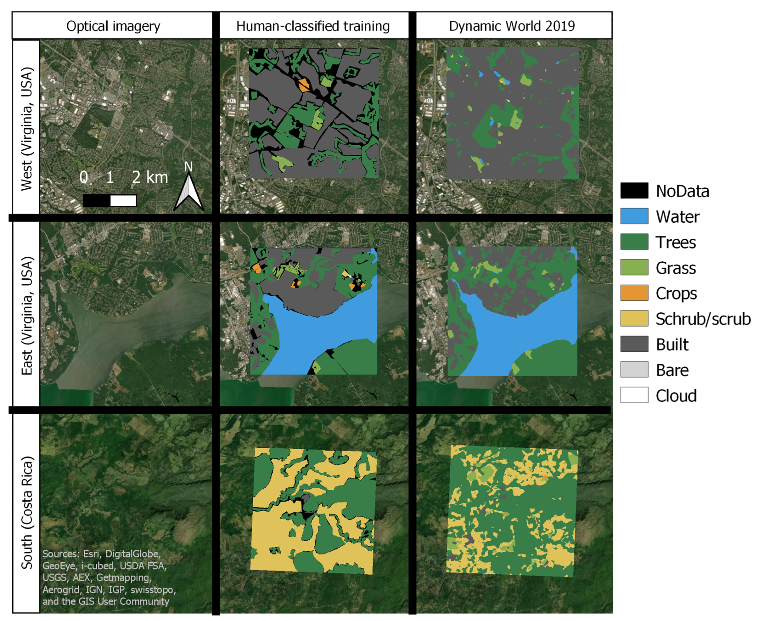
2.4.1. Transferability Evaluation

To further validate the subclassifications and evaluate how transferrable the thresholds are between watersheds, we trained built and tree probability thresholds on the Rock Creek and South Fork Quantico Creek Watersheds and then transferred them to the Bush Creek Watershed that had not been trained for. We then evaluated the subclassifications in the watershed not trained for using the same methods as above, by comparing proportions of total watershed land area and by calculating overall, user’s, and producer’s accuracies.

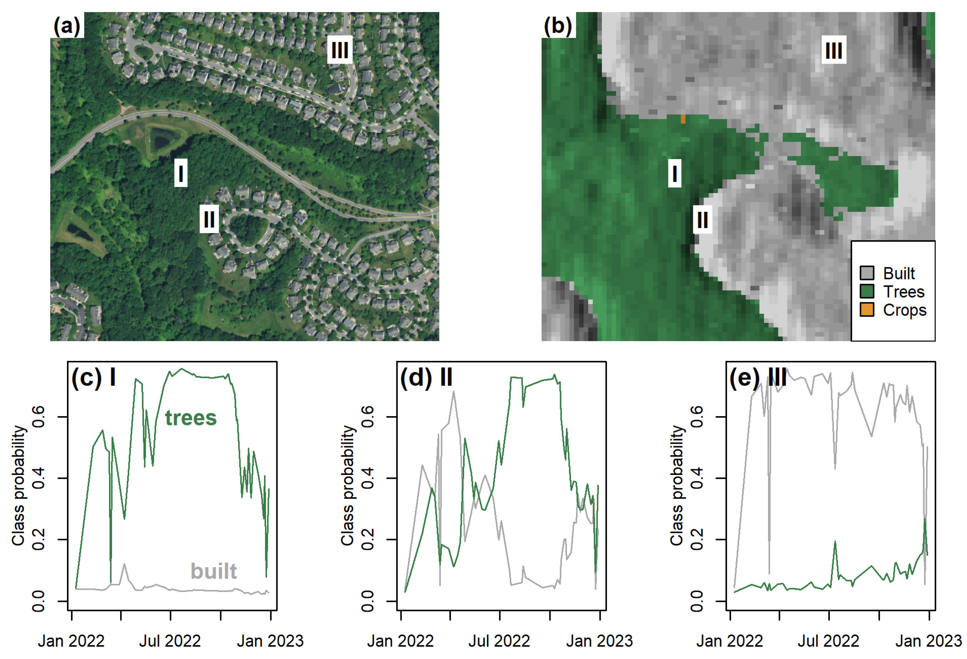
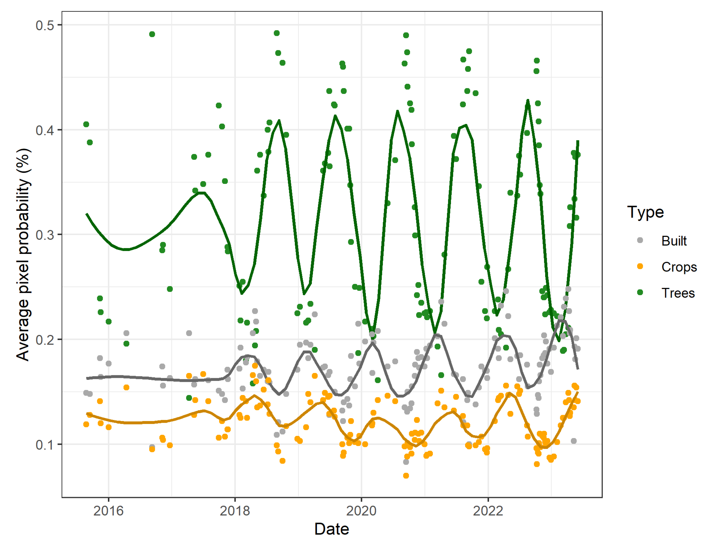
2.4.2. Temporal Variability Analysis

To provide insights on seasonal variability, we also analyzed variation in a time series of Dynamic World records for the Bush Creek Watershed (5 August 2015 to 13 June 2023), which constituted 143 Dynamic World records representing complete daily composites of the watershed and days with snow probabilities > 0.1 removed. This allowed us to visualize how seasonal cycles could lead to varying probabilities for trees and built area. The crops class was also included for reference. Loess smooth lines showing seasonal cycles were calculated using R package ggplot2 version 3.5.1 [50].

2.4.3. Human-Classified Validations

To evaluate how the accuracy of our approach may be affected by the accuracy of the primary Dynamic World classes prior to subclassification (trees, built, etc.), we compared Dynamic World 2019 dominant land cover composites (1 January to 31 December, 2019) with human-classified images from the Dynamic World training dataset, which had been classified off of Sentinel-2 imagery from 2019 [23,40]. We used three images that were all within 30 km of our study area (the South image in tropical Costa Rica: dw_-85.4393520175_10.7676075124-20190305, the East image in temperate Virginia: dw_-77.1067353418_38.6996057874-20191001, and the West image in temperate Virginia: dw_-77.3966281551_39.0206632388-20190524) that covered forest and developed landscapes. We evaluated the classifications against this human reference by calculating overall, user’s, and producer’s accuracies.

3. Results

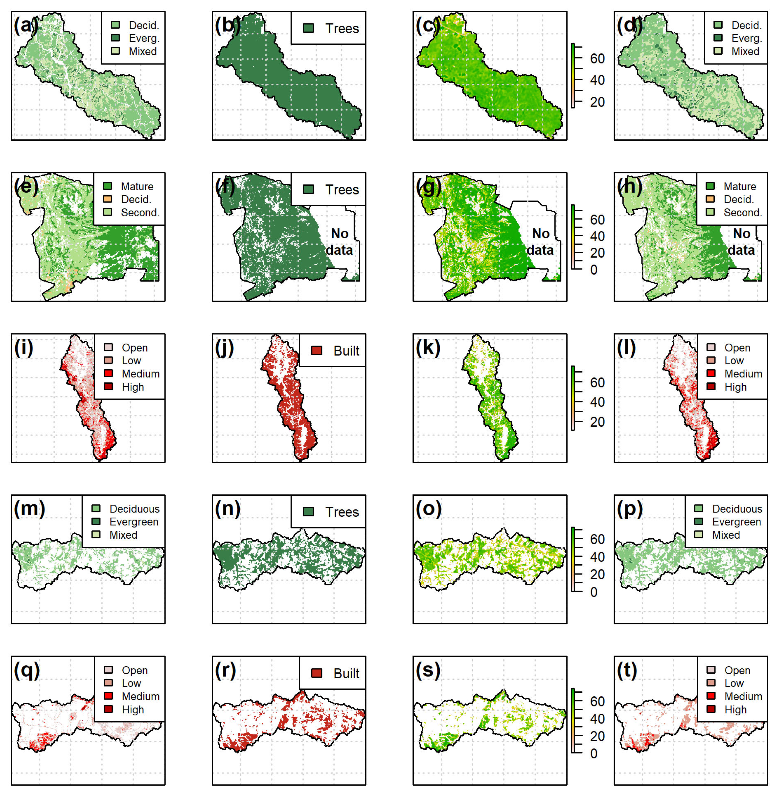
3.1. Subclassifications for Temperate Forest, Tropical Forest, and Developed Land

The Dynamic World 2022 composite trees class does not capture the variability in forest types in the temperate forested South Fork Quantico Creek watershed, whereas NLCD 2019 does. However, there was spatial variation in Dynamic World trees class probability that ranged from low to high probabilities (~0.40 to ~0.70) and reflected forest type variation well (Figure 4a–c). To subclassify this temperate forest using the class probability information, we assigned a probability of >0.65 as evergreen, 0.62 to 0.65 as mixed forest, and <0.62 as deciduous forest, following our one-at-a-time approach described earlier. The approach identified patches of evergreen forest among the mixed and deciduous stands that also show up in NLCD 2019, while also capturing the dominance of deciduous and mixed forest types, with user’s accuracies ranging from 43 to 76%, and producer’s accuracies ranging from 50 to 70% (Figure 4d;

Table 2. Accuracy matrices comparing reference classes with classified Dynamic World data using pixel class probabilities, including producer’s, user’s, and overall accuracies (%), for (a) South Fork Quantico Creek Watershed, (b) Guanacaste National Park, (c) Rock Creek Watershed, and (d,e) Bush Creek Watershed. User’s accuracy is presented in the right column, producer’s accuracy is in the bottom row, and overall accuracy (OA) is in the bottom right cell. See Equations (1)–(3) for calculations.

(a) South Fork Quantico Creek Watershed
		Reference Data (NLCD)
		Deciduous	Mixed	Evergreen	Total	User’s Acc.
Dyn. World class probabilities	Deciduous	158,860	47,068	2252	208,180	76.31
	Mixed	66,364	66,077	8817	141,258	46.78
	Evergreen	2977	11,902	11,169	26,048	42.88
	Total	228,201	125,047	22,238	375,486	NA
	Prod’s Acc.	69.61	52.84	50.22	NA	OA: 62.88
(b) Guanacaste National Park
		Reference Data (SINAC)
		Deciduous	Secondary	Mature	Total	User’s Acc.
Dyn. World class probabilities	Deciduous	1575	40,308	782	42,665	3.69
	Secondary	43,338	983,435	192,831	1,219,604	80.64
	Mature	14	113,094	563,075	676,183	83.27
	Total	44,927	1,136,837	756,688	1,938,452	NA
	Prod’s Acc.	3.51	86.51	74.41	NA	OA: 79.86
(c) Rock Creek Watershed
		Reference Data (NLCD)
		Open Space	Low	Medium	High	Total	User’s Acc.
Dyn. World class probabilities	Open space	182,777	109,144	32,818	9787	334,526	54.64
	Low	133,273	241,728	93,835	41,247	510,083	47.39
	Medium	25,282	123,437	102,826	50,898	302,443	34
	High	2859	26,189	49,543	19,910	98,501	20.21
	Total	344,191	500,498	279,022	121,842	1245,553	NA
	Prod’s Acc.	53.1	48.3	36.85	16.34	NA	OA: 43.94
(d) Bush Creek Watershed Forest
		Reference Data (NLCD)
		Deciduous	Mixed	Evergreen	Total	User’s Acc.
Dyn. World class probabilities	Deciduous	348,631	36,677	1212	386,520	90.2
	Mixed	21,852	4,220	1321	27,393	15.41
	Evergreen	347	879	2365	3591	65.86
	Total	370,830	41,776	4898	417,504	NA
	Prod’s Acc.	94.01	10.1	48.29	NA	OA: 85.08
(e) Bush Creek Watershed Developed
		Reference Data (NLCD)
		Open Space	Low	Medium	High	Total	User’s Acc.
Dyn. World class probabilities	Open space	83,186	34,305	13,122	2745	133,358	62.38
	Low	27,534	29,600	20,299	3601	81,034	36.53
	Medium	2406	6818	14,523	3379	27,126	53.54
	High	68	411	1228	629	2336	26.93
	Total	113,194	71,134	49,172	10,354	243,854	NA
	Prod’s Acc.	73.49	41.61	29.54	6.07	NA	OA: 52.46

a). Differences in proportions of watershed areas reflected the overall difference in tree cover simulation between the datasets (for instance, the watershed was 52.5% deciduous forest in NLCD 2019 and 57.0% deciduous forest in Dynamic World 2022;

Table 3. Proportions of total area from reference data (NLCD, SINAC) and Dynamic World 2022 classified by class probabilities for (a) South Fork Quantico Creek Watershed, (b) Guanacaste National Park, (c) Rock Creek Watershed, and (d,e) Bush Creek Watershed. See Equation (4) for the calculation.

(a) S.F. Quantico Creek Watershed
Class	NLCD (%)	DW (%)
Evergreen	5.1	6.2
Mixed	28.8	35.4
Deciduous	52.5	57
All forest	86.3	98.6
(b) Guanacaste National Park
Class	SINAC (%)	DW (%)
Deciduous	2.3	2.5
Mature	28.6	27.5
Secondary	48.3	54.4
All forest	79.2	84.4
(c) Rock Creek Watershed
Class	NLCD (%)	DW (%)
High	6.2	4.9
Med	14.4	15.2
Low	26.6	26.1
Open	26.6	19.3
All developed	73.7	65.6
(d) Bush Creek Watershed Forest
Class	NLCD (%)	DW (%)
Evergreen	0.4	0.3
Mixed	3.3	2.4
Deciduous	27.9	47.5
All forest	31.5	50.2
(e) Bush Creek Watershed Developed
Class	NLCD (%)	DW (%)
High	0.8	0.2
Med	4.2	2.2
Low	7.4	7.3
Open	17.5	14.2
All developed	29.8	24

a).

For the tropical forested Guanacaste National Park, Dynamic World 2022 trees class probabilities showed spatial variation which reflected differences in mature and secondary forest shown in the SINAC 2019 data, although there was a “no data” area in the mountainous eastern side of the park where it appeared high cloud cover may interfere with the ability of the classifier (Figure 4e–g). To subclassify this tropical forest using class probability information, we arrived on probabilities of >0.71 for mature forest, 0.35 to 0.71 for secondary forest, and <0.35 for deciduous forest, which led to an overall accuracy of 80% and proportions of watershed area within a few percentage points (Figure 4h; Table 2b and Table 3b). However, the approach was not able to distinguish deciduous forest from the other forest types, with producer’s and user’s accuracies of only 4%. This may be due to the small number of overall pixels that came from deciduous (2.3% of the total number of pixels), combined with mixing with secondary or mature types.

For subclassifying developed areas of the Rock Creek Watershed using Dynamic World 2022, we arrived on class probability criteria of >0.70 for high-intensity, 0.67 to 0.70 for medium intensity, 0.54 to 0.66 for low intensity, and <0.54 for open space developments, which produced a developed subclassification that showed the spatial variation in developed area of the NLCD, and more detail than the default “built area” class of Dynamic World (Figure 4i–l). However, accuracies were generally lower than those for the forest classifications, with an overall accuracy of only 44% (Table 2c). One difference was that the NLCD 2019 simulated more overall open space (26.6%) than the Dynamic World pixel class probability approach (19.3%), causing NLCD 2019 to estimate a higher overall amount of developed area in the watershed (Table 3c). Also, the original 30 m pixel size of the NLCD was unable to identify fine-scale differences in developed intensities present within the pixel, while the 10 m size of Dynamic World 2022 pixels was able to distinguish these finer differences in developed type (example in Figure S2).

3.2. Evaluation of Transferability and Human-Classified Reference

By transferring the temperate forest and developed type probability thresholds from the previous section to a watershed they were not trained on (Bush Creek), there was an overall accuracy for temperate forest types of 85%, and for developed area types of 52%, which was comparable to the South Fork Quantico Creek and Rock Creek Watershed accuracies (Table 2d,e). The subclassification represented that most of the trees are deciduous (Figure 4m–p) and most of the built area is low- to medium-intensity residential areas (Figure 4q–t). These were similar conclusions as the NLCD, although the NLCD tended to estimate more developed area and less forest overall (Table 3d,e).

When examining a complete time series of Dynamic World pixel class probability data for the Bush Creek Watershed (5 August 2015 to 13 June 2023), we discovered seasonal variation in pixel class probabilities that would likely make transferring thresholds from different seasons difficult. For instance, the watershed-average trees probability would cycle from approximately 0.2–0.3 during the winter to 0.4–0.5 during the summer, while the typical built probability would cycle from approximately 0.1 during summer to 0.2 during winter (Figure 5).

Overall accuracies for the Dynamic World 2019 composite with original classification scheme in matching the classification of the human-referenced training data were 90% for the East image in temperate Virginia, USA, 89% for the West image in temperate Virginia, USA, and 69% for the South image in tropical Costa Rica (Figure 6, Tables S3–S5). In the temperate images, user’s and producer’s accuracies for classifying a pixel as trees ranged from 71% to 94%, and accuracies for classifying a pixel as built area ranged from 78% to 98% (Tables S3 and S4). In the tropical image, the producer’s accuracy for classifying trees was 95%, while the user’s accuracy was 64% (Table S5). There was only a small portion of the tropical image area classified as built in the training data (0.4%).

4. Discussion

By distinguishing mature and secondary tropical forest using the CNN-based class probability approach, Dynamic World class probabilities may be more useful for biodiversity models of tree species richness and composition (e.g., [51,52]), or ecohydrological investigations, than the aggregate “trees” class common in global land cover datasets and the primary Dynamic World classification. Further, distinguishing developed land cover types and intensities using class probabilities could allow for more precise simulation of urbanization impacts to water quality by models that can distinguish different developed land uses in watersheds other than the aggregate “built” land cover class. Future work should investigate the sensitivity of class probability thresholds and their impacts in model applications such as these, particularly with regard to classification accuracies, as inconsistent classifications could affect model outputs and have real-world decision making implications [53,54].

One factor affecting the reported accuracy of our classifications was the different spatial resolution of our reference data. Incorporating subdominant classes allows our accuracy matrices to be more representative of the agreement between our classification and reference data [49]. However, the nine heterogeneous 10 m Dynamic World pixels in one 30 m NLCD pixel implies that the greatest achievable accuracy metric is depreciated by the amount of heterogeneity within the finer (Dynamic World) pixels [49]. For example, if the NLCD pixel was classified as mixed forest, and the finer Dynamic World pixels within it were subclassified as deciduous, evergreen, and mixed forests, the Dynamic World subclassification would technically be correct. However, resampling to either the finer or coarser resolution dataset could result in comparisons of either deciduous-to-mixed or evergreen-to-mixed, which the accuracy matrix would wrongly declare as incorrect. Resampling the Dynamic World probabilities to the NLCD resolution by averaging them did not improve the accuracy for forested or developed classifications, likely for the same reasons (Tables S1 and S2). It has been previously shown that the resolution of the NLCD can lead to biases in urban areas where land cover is spatially heterogeneous at a fine scale, such as lawn-dominated suburbs [55], which is likely lowering calculated accuracies. Thus, the maximum accuracy the matrix could achieve would be lower [49].

A second factor related to the accuracy of this approach is the training of the nine primary Dynamic World classes using the Dynamic World Training Dataset. Although the Dynamic World CNN model performs well for correctly classifying land cover overall in these training images with high accuracy, a significant portion of each image was classified as “no data” in the training images, as high as 19% of total area in the temperate West image (Figure 6, middle column). This could affect these accuracy calculations, as the “no data” classifications were non-randomly distributed and occurred on roads, fields, and edges between classified parcels, where we generally found lower confidences in classifying land cover in our study area (e.g., Figure 2d). Previous research has shown that, for example, pixels located near the boundary between two land cover types (e.g., the edge between a built area and a forest) can have lower class probabilities than pixels located within the core of a land cover parcel (i.e., homogenous group of pixels) [56,57]. Further, previous investigation in our study areas has found that seasonal classification inconsistencies in these edges and low-confidence areas can affect estimates of land cover change that then impact the simulations of hydrologic and water quality models based on the data [53].

Thus, there are implications for using remotely sensed CNN-based approaches such as the Dynamic World dataset. Although there can be inconsistencies compared with human-classified images, using the CNN-based Dynamic World class probabilities creates access to high resolution land cover data covering the globe with high temporal frequency, making the data accessible to a large number of users in different regions and improving equity in access to land cover information [23,24]. To strengthen this benefit, the lower confidence in classifying edges between classified parcels implies that further research is needed to alleviate confusion in classifying land cover in heterogenous edge zones, especially considering the influence of seasonal vegetation phenology [31,32,33]. Additionally, the fringes between urban areas and more natural land cover types like forests, where we generally found lower pixel class probabilities averaged over the year, are important for ecosystem resilience and productivity [58]. Variation in Dynamic World class probabilities would be useful for identifying these ecologically valuable areas.

A third factor related to the accuracy of this approach is clouds, which obscured the eastern portion of Guanacaste National Park from our analyses, and would cause problems for implementing a pixel class probability-based classification in other very cloudy areas. Cloud cover presents challenges with all visual-based classification approaches in the tropics [59].

The variation in land cover probabilities over time that we identified for the Bush Creek Watershed, such as trees probability cycling from 0.2–0.3 to 0.4–0.5 throughout the year, is likely due to spatiotemporal inconsistencies in classification [60], such as seasonal variation [53]. For analyses involving time series of high-frequency pixel class probabilities, approaches should be implemented to address spurious or illogical changes due to inconsistencies between land cover images [61,62,63]. Researchers could explore using tools such as TIMESAT to investigate relationships between vegetation phenology and seasonality of the land cover time series and enhance classifications [64,65]. It is possible that different time series of land cover data, such as seasonal comparisons, could further be used to subclassify agricultural land (e.g., [66]).

Limitations of the Study

In addition to the considerations of accuracy discussed above, the class probability subclassification approach using the global Dynamic World land cover product could have additional limitations that are important to note. First, different land cover products have different classification schemes [57], which could create confusion when assigning class probability thresholds based on other reference schemes. Second, researchers using the global, thematically detailed data could encounter limited data for ground truthing or real data validations matching their areas and needs, which could require additional work to ensure reliable classifications. One way to get around these limitations could be by fusing results with other complementary land cover products available in the study area [31]. Finally, while our study explored increasing the thematic details of a global land cover dataset in temperate forest, tropical forest, and developed study cases, future work is suggested to expand and evaluate the approach in other landscapes such as agricultural regions and different biomes, including additional land cover types beyond trees and built area.

5. Conclusions

This study explored the use of CNN-based pixel class probability outputs of the Dynamic World global land cover dataset to create customizable schemes that could meet the needs of researchers and conservationists in regions where recent (e.g., less than a year old) products with high thematic resolution are not readily available. We demonstrated the capabilities of pixel class probabilities in developed and temperate forest watersheds of the eastern United States, as well as a tropical forest area in Costa Rica, to be used to provide moderate-to-excellent land cover classifications. By using annual composites, we successfully transferred a classification scheme to another watershed without loss of accuracy. We expect that the greatest impact of this approach could be outside the USA and Europe where detailed, high-frequency land cover classifications are less common. Future work should explore class probabilities for other biomes, seasonal time periods, and for agricultural land cover types. As the data for these investigations are already available through the Dynamic World dataset on Google Earth Engine, the pixel class probabilities can facilitate the generation of purpose-specific land cover classifications for environmental models.

References

1. Akkermans, T.; Van Rompaey, A.; Van Lipzig, N.; Moonen, P.; Verbist, B. Quantifying Successional Land Cover after Clearing of Tropical Rainforest along Forest Frontiers in the Congo Basin. Phys. Geogr. 2013, 34, 417–440. [Google Scholar] [CrossRef]
2. Duan, Y.; Akula, S.; Kumar, S.; Lee, W.; Khajehei, S. A Hybrid Physics–AI Model to Improve Hydrological Forecasts. Artif. Intell. Earth Syst. 2023, 2, e220023. [Google Scholar] [CrossRef]
3. Fu, B.; Merritt, W.S.; Croke, B.F.W.; Weber, T.R.; Jakeman, A.J. A Review of Catchment-Scale Water Quality and Erosion Models and a Synthesis of Future Prospects. Environ. Model. Softw. 2019, 114, 75–97. [Google Scholar] [CrossRef]
4. Massoud, E.C.; Hoffman, F.; Shi, Z.; Tang, J.; Alhajjar, E.; Barnes, M.; Braghiere, R.K.; Cardon, Z.; Collier, N.; Crompton, O.; et al. Perspectives on Artificial Intelligence for Predictions in Ecohydrology. Artif. Intell. Earth Syst. 2023, 2, e230005. [Google Scholar] [CrossRef]
5. Yao, S.; Chen, C.; He, M.; Cui, Z.; Mo, K.; Pang, R.; Chen, Q. Land Use as an Important Indicator for Water Quality Prediction in a Region under Rapid Urbanization. Ecol. Indic. 2023, 146, 109768. [Google Scholar] [CrossRef]
6. Arnold, J.G.; Srinivasan, R.; Muttiah, R.S.; Williams, J.R. Large Area Hydrologic Modeling and Assessment Part I: Model Development. JAWRA J. Am. Water Resour. Assoc. 1998, 34, 73–89. [Google Scholar] [CrossRef]
7. Haith, D.A.; Shoemaker, L.L. Generalized Watershed Loading Functions for Stream Flow Nutrients. JAWRA J. Am. Water Resour. Assoc. 1987, 23, 471–478. [Google Scholar] [CrossRef]
8. Yang, L.; Jin, S.; Danielson, P.; Homer, C.; Gass, L.; Bender, S.M.; Case, A.; Costello, C.; Dewitz, J.; Fry, J.; et al. A New Generation of the United States National Land Cover Database: Requirements, Research Priorities, Design, and Implementation Strategies. ISPRS J. Photogramm. Remote Sens. 2018, 146, 108–123. [Google Scholar] [CrossRef]
9. Boryan, C.; Yang, Z.; Mueller, R.; Craig, M. Monitoring US Agriculture: The US Department of Agriculture, National Agricultural Statistics Service, Cropland Data Layer Program. Geocarto Int. 2011, 26, 341–358. [Google Scholar] [CrossRef]
10. Liang, S.; He, T.; Huang, J.; Jia, A.; Zhang, Y.; Cao, Y.; Chen, X.; Chen, X.; Cheng, J.; Jiang, B. Advances in High-Resolution Land Surface Satellite Products: A Comprehensive Review of Inversion Algorithms, Products and Challenges. Sci. Remote Sens. 2024, 10, 100152. [Google Scholar] [CrossRef]
11. Xu, P.; Tsendbazar, N.-E.; Herold, M.; de Bruin, S.; Koopmans, M.; Birch, T.; Carter, S.; Fritz, S.; Lesiv, M.; Mazur, E. Comparative Validation of Recent 10 M-Resolution Global Land Cover Maps. Remote Sens. Env. 2024, 311, 114316. [Google Scholar] [CrossRef]
12. Zanaga, D.; Van De Kerchove, R.; Daems, D.; De Keersmaecker, W.; Brockmann, C.; Kirches, G.; Wevers, J.; Cartus, O.; Santoro, M.; Fritz, S. ESA WorldCover 10 m 2021 V200, Version v200; ESA: Paris, France, 2022. [Google Scholar] [CrossRef]
13. Zanaga, D.; Van De Kerchove, R.; De Keersmaecker, W.; Souverijns, N.; Brockmann, C.; Quast, R.; Wevers, J.; Grosu, A.; Paccini, A.; Vergnaud, S.; et al. ESA WorldCover 10 m 2020 V100, Version V100; ESA: Paris, France, 2022. [Google Scholar]
14. Auerbach, D.A.; Buchanan, B.P.; Alexiades, A.V.; Anderson, E.P.; Encalada, A.C.; Larson, E.I.; McManamay, R.A.; Poe, G.L.; Walter, M.T.; Flecker, A.S. Towards Catchment Classification in Data-Scarce Regions. Ecohydrology 2016, 9, 1235–1247. [Google Scholar] [CrossRef]
15. de Lima, R.A.F.; Phillips, O.L.; Duque, A.; Tello, J.S.; Davies, S.J.; de Oliveira, A.A.; Muller, S.; Honorio Coronado, E.N.; Vilanova, E.; Cuni-Sanchez, A.; et al. Making Forest Data Fair and Open. Nat. Ecol. Evol. 2022, 6, 656–658. [Google Scholar] [CrossRef] [PubMed]
16. Pandeya, B.; Buytaert, W.; Zulkafli, Z.; Karpouzoglou, T.; Mao, F.; Hannah, D.M. A Comparative Analysis of Ecosystem Services Valuation Approaches for Application at the Local Scale and in Data Scarce Regions. Ecosyst. Serv. 2016, 22, 250–259. [Google Scholar] [CrossRef]
17. Wagner, P.D.; Fiener, P.; Wilken, F.; Kumar, S.; Schneider, K. Comparison and Evaluation of Spatial Interpolation Schemes for Daily Rainfall in Data Scarce Regions. J. Hydrol. 2012, 464–465, 388–400. [Google Scholar] [CrossRef]
18. Stanimirova, R.; Tarrio, K.; Turlej, K.; McAvoy, K.; Stonebrook, S.; Hu, K.-T.; Arévalo, P.; Bullock, E.L.; Zhang, Y.; Woodcock, C.E.; et al. A Global Land Cover Training Dataset from 1984 to 2020. Sci. Data 2023, 10, 879. [Google Scholar] [CrossRef] [PubMed]
19. Zhang, H.K.; Roy, D.P.; Luo, D. Demonstration of Large Area Land Cover Classification with a One Dimensional Convolutional Neural Network Applied to Single Pixel Temporal Metric Percentiles. Remote Sens. Environ. 2023, 295, 113653. [Google Scholar] [CrossRef]
20. Kolarik, N.E.; Roopsind, A.; Pickens, A.; Brandt, J.S. A Satellite-Based Monitoring System for Quantifying Surface Water and Mesic Vegetation Dynamics in a Semi-Arid Region. Ecol. Indic. 2023, 147, 109965. [Google Scholar] [CrossRef]
21. Cardille, J.A.; Fortin, J.A. Bayesian Updating of Land-Cover Estimates in a Data-Rich Environment. Remote Sens. Environ. 2016, 186, 234–249. [Google Scholar] [CrossRef]
22. Pasquarella, V.J.; Arévalo, P.; Bratley, K.H.; Bullock, E.L.; Gorelick, N.; Yang, Z.; Kennedy, R.E. Demystifying LandTrendr and CCDC Temporal Segmentation. Int. J. Appl. Earth Obs. Geoinf. 2022, 110, 102806. [Google Scholar] [CrossRef]
23. Brown, C.F.; Brumby, S.P.; Guzder-Williams, B.; Birch, T.; Hyde, S.B.; Mazzariello, J.; Czerwinski, W.; Pasquarella, V.J.; Haertel, R.; Ilyushchenko, S.; et al. Dynamic World, Near Real-Time Global 10 m Land Use Land Cover Mapping. Sci. Data 2022, 9, 251. [Google Scholar] [CrossRef]
24. Venter, Z.S.; Barton, D.N.; Chakraborty, T.; Simensen, T.; Singh, G. Global 10 m Land Use Land Cover Datasets: A Comparison of Dynamic World, World Cover and Esri Land Cover. Remote Sens. 2022, 14, 4101. [Google Scholar] [CrossRef]
25. Sales, M.H.R.; De Bruin, S.; Souza, C.; Herold, M. Land Use and Land Cover Area Estimates from Class Membership Probability of a Random Forest Classification. IEEE Trans. Geosci. Remote Sens. 2021, 60, 4402711. [Google Scholar] [CrossRef]
26. Wang, X.; Zhang, Y.; Zhang, K. Automatic 10 m Forest Cover Mapping in 2020 at China’s Han River Basin by Fusing ESA Sentinel-1/Sentinel-2 Land Cover and Sentinel-2 near Real-Time Forest Cover Possibility. Forests 2023, 14, 1133. [Google Scholar] [CrossRef]
27. Boucher, A.; Seto, K.C.; Journel, A.G. A Novel Method for Mapping Land Cover Changes: Incorporating Time and Space with Geostatistics. IEEE Trans. Geosci. Remote Sens. 2006, 44, 3427–3435. [Google Scholar] [CrossRef]
28. Khatami, R.; Mountrakis, G.; Stehman, S.V. Predicting Individual Pixel Error in Remote Sensing Soft Classification. Remote Sens. Environ. 2017, 199, 401–414. [Google Scholar] [CrossRef]
29. Small, C.; Sousa, D. Spectral Characteristics of the Dynamic World Land Cover Classification. Remote Sens. 2023, 15, 575. [Google Scholar] [CrossRef]
30. Venter, Z.S.; Roos, R.E.; Nowell, M.S.; Rusch, G.M.; Kvifte, G.M.; Sydenham, M.A.K. Comparing Global Sentinel-2 Land Cover Maps for Regional Species Distribution Modeling. Remote Sens. 2023, 15, 1749. [Google Scholar] [CrossRef]
31. Zhang, W.; Wang, J.; Lin, H.; Cong, M.; Wan, Y.; Zhang, J. Fusing Multiple Land Cover Products Based on Locally Estimated Map-Reference Cover Type Transition Probabilities. Remote Sens. 2023, 15, 481. [Google Scholar] [CrossRef]
32. Eliades, M.; Neophytides, S.; Mavrovouniotis, M.; Panagiotou, C.F.; Anastasiadou, M.N.; Varvaris, I.; Papoutsa, C.; Bachofer, F.; Michaelides, S.; Hadjimitsis, D. Temporal Dynamics of Global Barren Areas between 2001 and 2022 Derived from MODIS Land Cover Products. Remote Sens. 2024, 16, 3317. [Google Scholar] [CrossRef]
33. Boston, T.; Van Dijk, A.; Thackway, R. Convolutional Neural Network Shows Greater Spatial and Temporal Stability in Multi-Annual Land Cover Mapping Than Pixel-Based Methods. Remote Sens. 2023, 15, 2132. [Google Scholar] [CrossRef]
34. Ramachandra, T.V.; Negi, P.; Mondal, T.; Ahmed, S.A. Insights into the Linkages of Forest Structure Dynamics with Ecosystem Services. Sci. Rep. 2025, 15, 15606. [Google Scholar] [CrossRef] [PubMed]
35. Deng, Y.; Chen, G.; Tang, B.; Duan, X.; Zuo, L.; Zhao, H. Study on Class Imbalance in Land Use Classification for Soil Erosion in Dry–Hot Valley Regions. Remote Sens. 2025, 17, 1628. [Google Scholar] [CrossRef]
36. USGS GAP. Protected Areas Database of the United States (PAD-US) 3.0 (Ver. 2.0, March 2023); USGS: Reston, VA, USA, 2022. [Google Scholar] [CrossRef]
37. Google. Google Satellite Basemap for South Fork Quantico Creek Watershed, Rock Creek Watershed, Bush Creek Watershed, Guanacaste National Park, and Western Hemisphere. Available online: https://developers.google.com/maps/documentation/javascript/maptypes (accessed on 2 June 2023).
38. Ebrahimy, H.; Mirbagheri, B.; Matkan, A.A.; Azadbakht, M. Per-Pixel Land Cover Accuracy Prediction: A Random Forest-Based Method with Limited Reference Sample Data. ISPRS J. Photogramm. Remote Sens. 2021, 172, 17–27. [Google Scholar] [CrossRef]
39. SINAC. Mature, Deciduous, and Secondary Forest; Costa Rica National System of Conservation Areas; SINAC: San José, Costa Rica, 2019. https://www.snitcr.go.cr/ico_servicios_ogc_info?k=bm9kbzo6NDA=&nombre=SINAC (accessed on 23 July 2025).
40. Tait, A.M.; Brumby, S.P.; Hyde, S.B.; Mazzariello, J.; Corcoran, M. Dynamic World Training Dataset for Global Land Use and Land Cover Categorization of Satellite Imagery [Dataset]. PANGAEA 2021, 933475. [Google Scholar] [CrossRef]
41. Bhosle, K.; Musande, V. Evaluation of Deep Learning CNN Model for Land Use Land Cover Classification and Crop Identification Using Hyperspectral Remote Sensing Images. J. Indian Soc. Remote Sens. 2019, 47, 1949–1958. [Google Scholar] [CrossRef]
42. Zhang, F.; Yan, M.; Hu, C.; Ni, J.; Zhou, Y. Integrating Coordinate Features in CNN-Based Remote Sensing Imagery Classification. IEEE Geosci. Remote Sens. Lett. 2021, 19, 5502505. [Google Scholar] [CrossRef]
43. Brown, C. Google/Dynamicworld: V1.0.0, Version 1.0.0.; Zenodo: Geneva, Switzerland, 2021. [Google Scholar] [CrossRef]
44. Frantz, D.; Haß, E.; Uhl, A.; Stoffels, J.; Hill, J. Improvement of the Fmask Algorithm for Sentinel-2 Images: Separating Clouds from Bright Surfaces Based on Parallax Effects. Remote Sens. Environ. 2018, 215, 471–481. [Google Scholar] [CrossRef]
45. European Space Agency. Sentinel-2: Cloud Probability. 2021. Available online: https://developers.google.com/earth-engine/datasets/catalog/COPERNICUS_S2_CLOUD_PROBABILITY (accessed on 23 July 2025).
46. Long, J.; Shelhamer, E.; Darrell, T. Fully Convolutional Networks for Semantic Segmentation. In Proceedings of the IEEE Computer Society Conference on Computer Vision and Pattern Recognition (CVPR), Boston, MA, USA, 7–12 June 2015; pp. 3431–3440. [Google Scholar] [CrossRef]
47. Naboureh, A.; Li, A.; Bian, J.; Lei, G. National Scale Land Cover Classification Using the Semiautomatic High-Quality Reference Sample Generation (HRSG) Method and an Adaptive Supervised Classification Scheme. IEEE J. Sel. Top. Appl. Earth Obs. Remote Sens. 2023, 16, 1858–1870. [Google Scholar] [CrossRef]
48. Maxwell, A.E.; Warner, T.A.; Guillén, L.A. Accuracy Assessment in Convolutional Neural Network-Based Deep Learning Remote Sensing Studies—Part 1: Literature Review. Remote Sens. 2021, 13, 2450. [Google Scholar] [CrossRef]
49. Latifovic, R.; Olthof, I. Accuracy Assessment Using Sub-Pixel Fractional Error Matrices of Global Land Cover Products Derived from Satellite Data. Remote Sens. Environ. 2004, 90, 153–165. [Google Scholar] [CrossRef]
50. Wickham, H. Ggplot2: Elegant Graphics for Data Analysis; Springer: New York, NY, USA, 2016. [Google Scholar]
51. Orsi, F.; Church, R.L.; Geneletti, D. Restoring Forest Landscapes for Biodiversity Conservation and Rural Livelihoods: A Spatial Optimisation Model. Environ. Model. Softw. 2011, 26, 1622–1638. [Google Scholar] [CrossRef]
52. Rozendaal, D.M.A.; Bongers, F.; Aide, T.M.; Alvarez-Dávila, E.; Ascarrunz, N.; Balvanera, P.; Becknell, J.M.; Bentos, T.V.; Brancalion, P.H.S.; Cabral, G.A.L.; et al. Biodiversity Recovery of Neotropical Secondary Forests. Sci. Adv. 2019, 5, eaau3114. [Google Scholar] [CrossRef] [PubMed]
53. Myers, D.T.; Jones, D.; Oviedo-Vargas, D.; Schmit, J.P.; Ficklin, D.L.; Zhang, X. Seasonal Variation in Land Cover Estimates Reveals Sensitivities and Opportunities for Environmental Models. Hydrol. Earth Syst. Sci. 2024, 28, 5295–5310. [Google Scholar] [CrossRef]
54. Li, Y.; Chang, J.; Luo, L.; Wang, Y.; Guo, A.; Ma, F.; Fan, J. Spatiotemporal Impacts of Land Use Land Cover Changes on Hydrology from the Mechanism Perspective Using SWAT Model with Time-Varying Parameters. Hydrol. Res. 2019, 50, 244–261. [Google Scholar] [CrossRef]
55. Smith, M.L.; Zhou, W.; Cadenasso, M.; Grove, M.; Band, L.E. Evaluation of the National Land Cover Database for Hydrologic Applications in Urban and Suburban Baltimore, Maryland. JAWRA J. Am. Water Resour. Assoc. 2010, 46, 429–442. [Google Scholar] [CrossRef]
56. Dean, A.M.; Smith, G.M. An Evaluation of Per-Parcel Land Cover Mapping Using Maximum Likelihood Class Probabilities. Int. J. Remote Sens. 2003, 24, 2905–2920. [Google Scholar] [CrossRef]
57. Wang, Z.; Mountrakis, G. Accuracy Assessment of Eleven Medium Resolution Global and Regional Land Cover Land Use Products: A Case Study over the Conterminous United States. Remote Sens. 2023, 15, 3186. [Google Scholar] [CrossRef]
58. Sijing, X.; Gang, L.; Biao, M. Vulnerability Analysis of Land Ecosystem Considering Ecological Cost and Value: A Complex Network Approach. Ecol. Indic. 2023, 147, 109941. [Google Scholar] [CrossRef]
59. Shrestha, D.P.; Saepuloh, A.; van der Meer, F. Land Cover Classification in the Tropics, Solving the Problem of Cloud Covered Areas Using Topographic Parameters. Int. J. Appl. Earth Obs. Geoinf. 2019, 77, 84–93. [Google Scholar] [CrossRef]
60. Liu, S.; Su, H.; Cao, G.; Wang, S.; Guan, Q. Learning from Data: A Post Classification Method for Annual Land Cover Analysis in Urban Areas. ISPRS J. Photogramm. Remote Sens. 2019, 154, 202–215. [Google Scholar] [CrossRef]
61. Sexton, J.O.; Song, X.P.; Huang, C.; Channan, S.; Baker, M.E.; Townshend, J.R. Urban Growth of the Washington, D.C.-Baltimore, MD Metropolitan Region from 1984 to 2010 by Annual, Landsat-Based Estimates of Impervious Cover. Remote Sens. Environ. 2013, 129, 42–53. [Google Scholar] [CrossRef]
62. Zhao, K.; Wulder, M.A.; Hu, T.; Bright, R.; Wu, Q.; Qin, H.; Li, Y.; Toman, E.; Mallick, B.; Zhang, X.; et al. Detecting Change-Point, Trend, and Seasonality in Satellite Time Series Data to Track Abrupt Changes and Nonlinear Dynamics: A Bayesian Ensemble Algorithm. Remote Sens. Environ. 2019, 232, 111181. [Google Scholar] [CrossRef]
63. Zhu, Z.; Woodcock, C.E. Continuous Change Detection and Classification of Land Cover Using All Available Landsat Data. Remote Sens. Environ. 2014, 144, 152–171. [Google Scholar] [CrossRef]
64. Jönsson, P.; Eklundh, L. TIMESAT—A Program for Analyzing Time-Series of Satellite Sensor Data. Comput. Geosci. 2004, 30, 833–845. [Google Scholar] [CrossRef]
65. Eklundh, L.; Jönsson, P. TIMESAT: A Software Package for Time-Series Processing and Assessment of Vegetation Dynamics. In Remote Sensing and Digital Image Processing; Springer: Berlin/Heidelberg, Germany, 2015; Volume 22. [Google Scholar]
66. Karra, K.; Kontgis, C.; Statman-Weil, Z.; Mazzariello, J.C.; Mathis, M.; Brumby, S.P. Global Landuse/Landcover with Sentinel 2 and Deep Learning. In Proceedings of the International Geoscience and Remote Sensing Symposium (IGARSS), Brussels, Belgium, 11–16 July 2021; Volume 2021. [Google Scholar]
67. Myers, D.; Oviedo-Vargas, D.; Daniels, M.; Aryal, Y. Pixel Class Probabilities Investigations Data [Dataset]; Version 1; Mendeley Data: London, UK, 2023. [Google Scholar] [CrossRef]
Figure 1. Study area map including (a) Rock Creek Watershed, (b) South Fork Quantico Creek Watershed, (c) Bush Creek Watershed, (d) Guanacaste National Park, and (e) reference map over Google satellite imagery [37]. Study areas are delineated with white borders, while locations in the reference map are red dots.
Remotesensing 17 02570 g001
Figure 2. Demonstration time series of pixel class probabilities for a mixed residential-forest area in the Bush Creek Watershed. (a) 2021 aerial imagery from the National Agricultural Imagery Program, (b) Dynamic World 2022 composite, with hillshade representing pixel probability, (c) Time series of pixel class probabilities for a high probability trees location (reference location I in panes above), (d) Time series of pixel class probabilities for a mixed trees/built location (reference location II in panes above), and (e) Time series of pixel class probabilities for a high probability built location (reference location III in panes above).
Remotesensing 17 02570 g002
Figure 3. Diagram of our experimental approach and purpose. NLCD: National Land Cover Database, SINAC: Costa Rica National System of Conservation Areas.
Remotesensing 17 02570 g003
Figure 4. For (ad) South Fork Quantico Creek Watershed forest types (top row), (eh) Guanacaste National Park forest types, (il) Rock Creek Watershed developed types, (mp) Bush Creek Watershed forest types, and (qt) Bush Creek Watershed developed types (bottom row): Reference land cover classes (left column), Dynamic World 2022 composite classifications, Dynamic World 2022 pixel class probabilities, and Dynamic World 2022 subclassified using class probabilities (right column).
Remotesensing 17 02570 g004
Figure 5. Time series of land cover class probabilities for the Bush Creek Watershed as spatial averages, showing seasonal variation, with loess smooth lines (n = 143 Dynamic World records representing complete daily composites of the watershed and days with snow probabilities > 0.1 removed).
Remotesensing 17 02570 g005
Figure 6. Display of ESRI optical imagery (left column), Dynamic World human-classified training dataset (middle column), and Dynamic World 2019 composite for three training locations (rows) over ESRI satellite imagery.
Remotesensing 17 02570 g006