
Remote Sensing Evidence of Blue Carbon Stock Increase and Attribution of Its Drivers in Coastal China


Abstract

1. Introduction
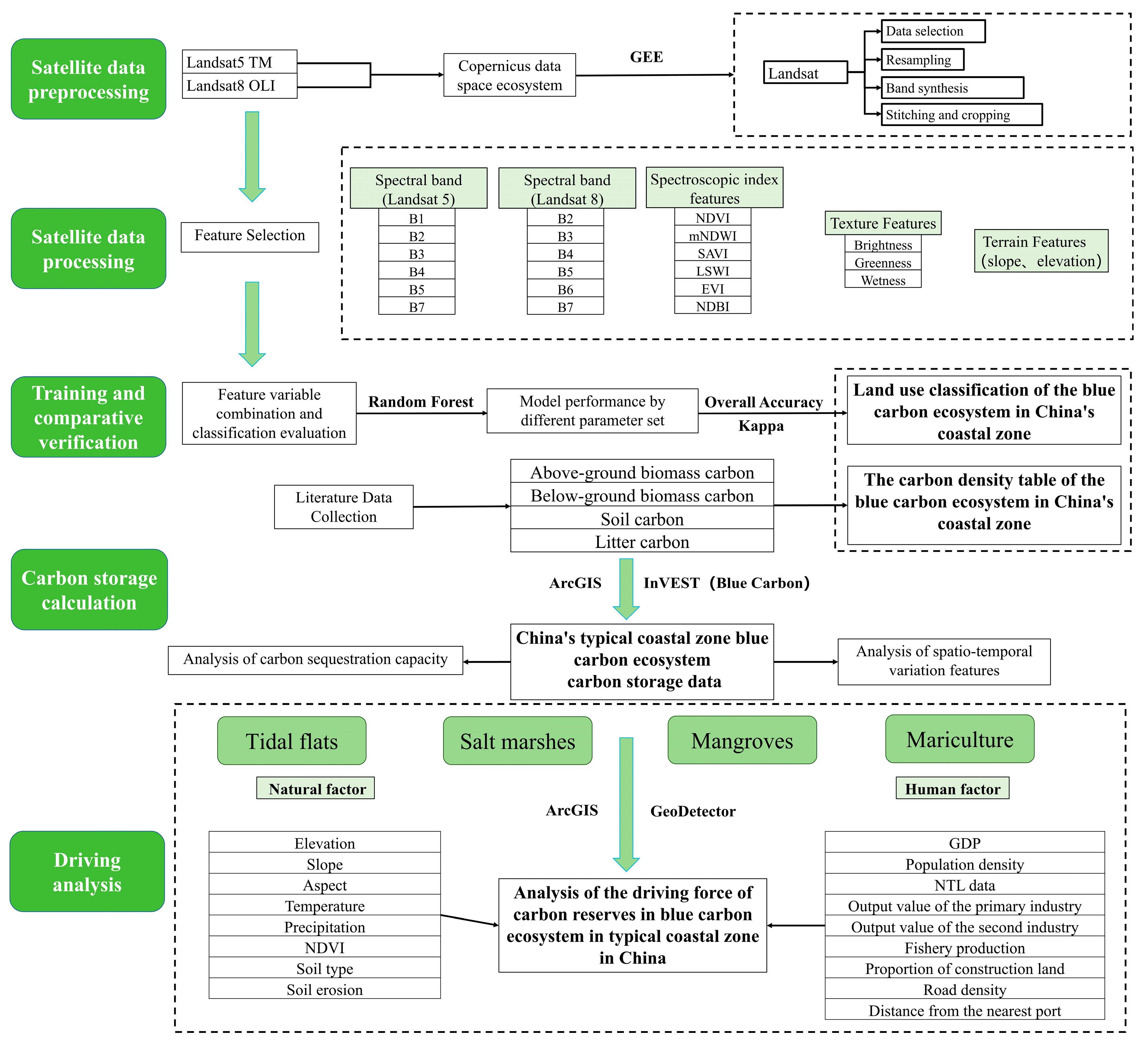
2. Materials and Methods
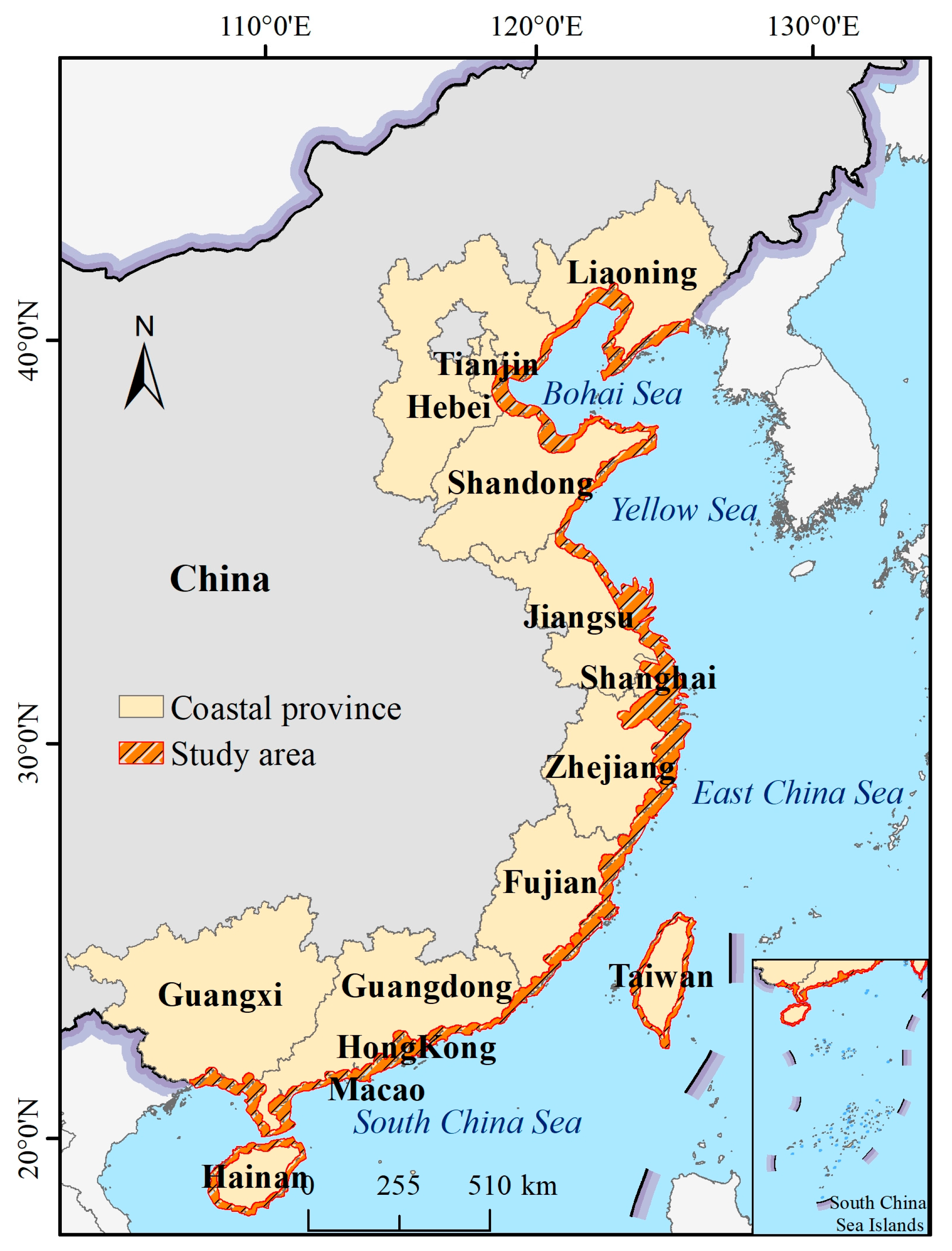
2.1. Materials
2.2. Methodology of Land Use Classification and Validation
2.2.1. Preprocessing and Land Use Classification of Remote Sensing Data
2.2.2. Extraction of Classification Feature Information
2.2.3. Random Forest-Based Classification and Accuracy Evaluation
2.3. Carbon Stock Estimation Based on the InVEST Model and Its Applicability
2.4. Driving Force Analysis of Carbon Stock Change Based on GeoDetector
3. Results
3.1. Classification of Land Use and Precision Assessment
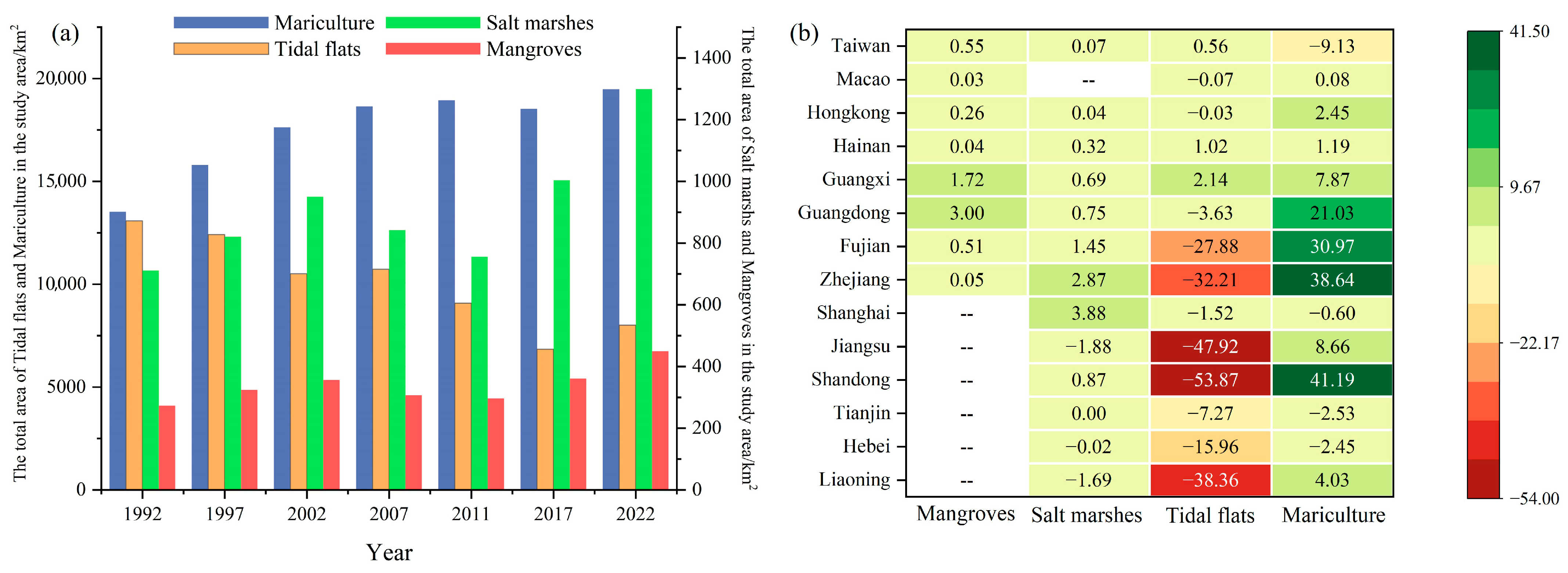
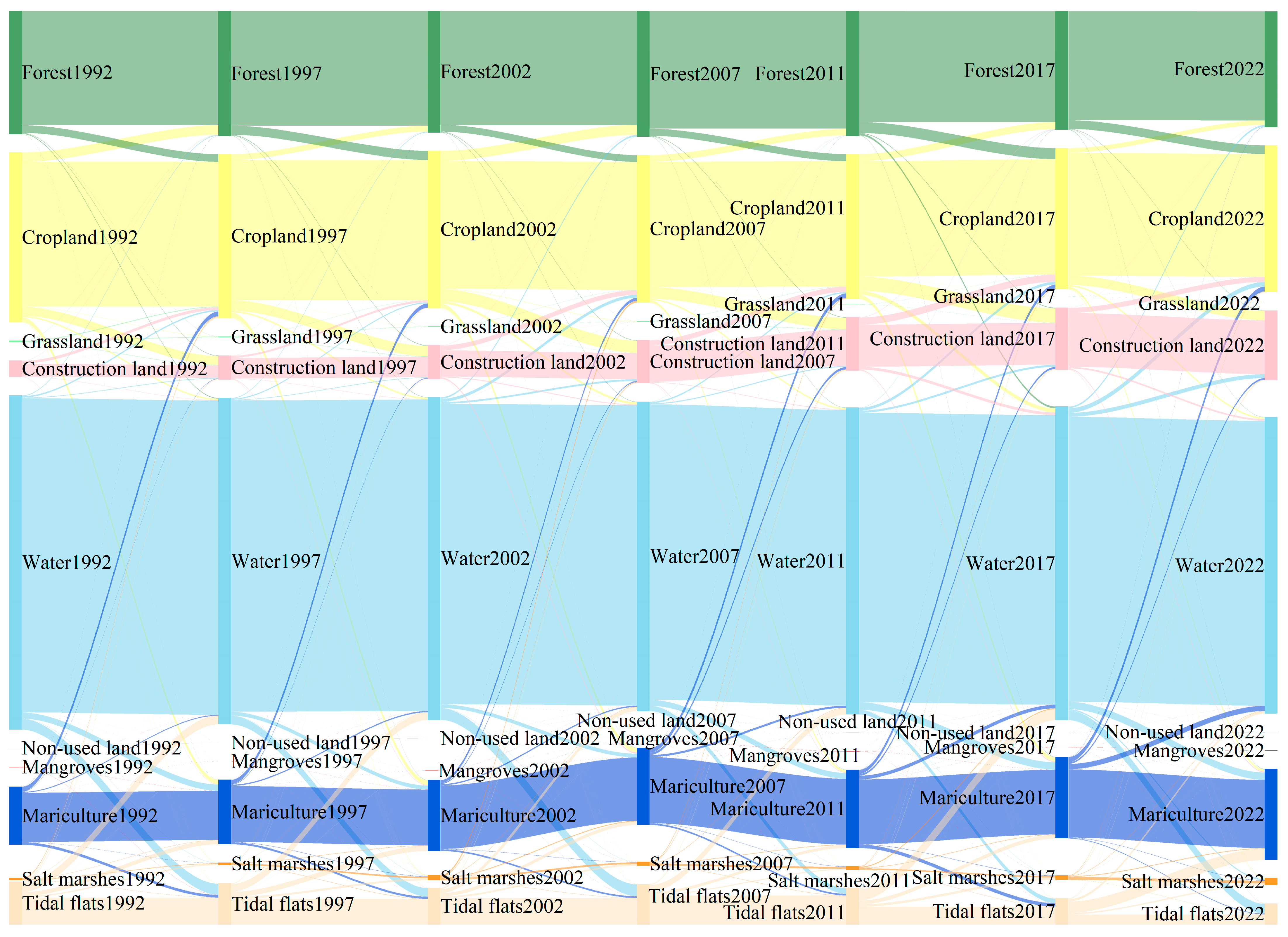
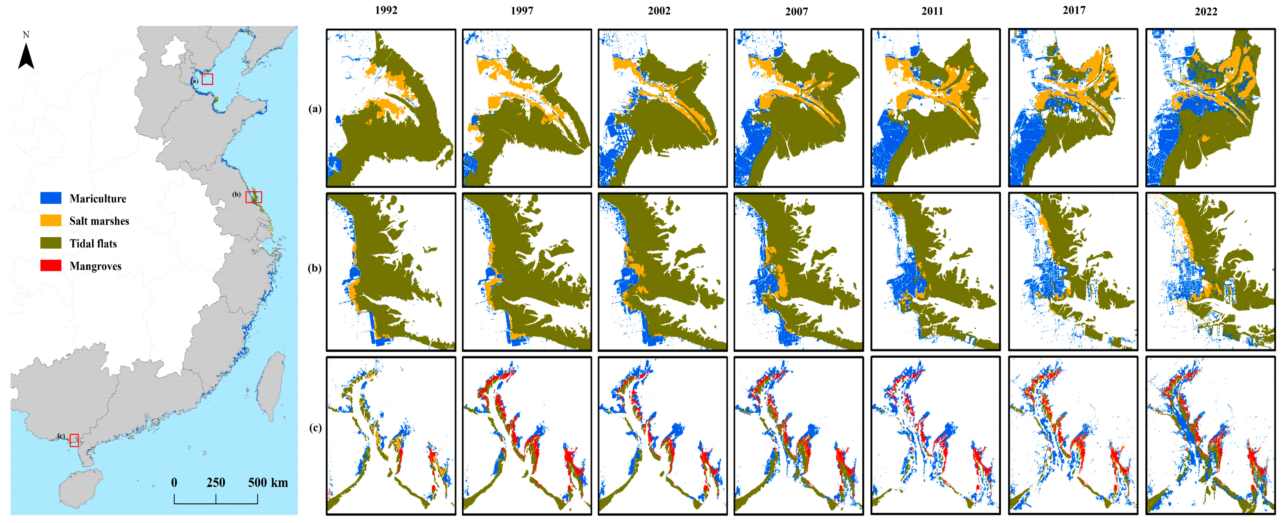
3.2. Spatiotemporal Pattern of Land Use Change
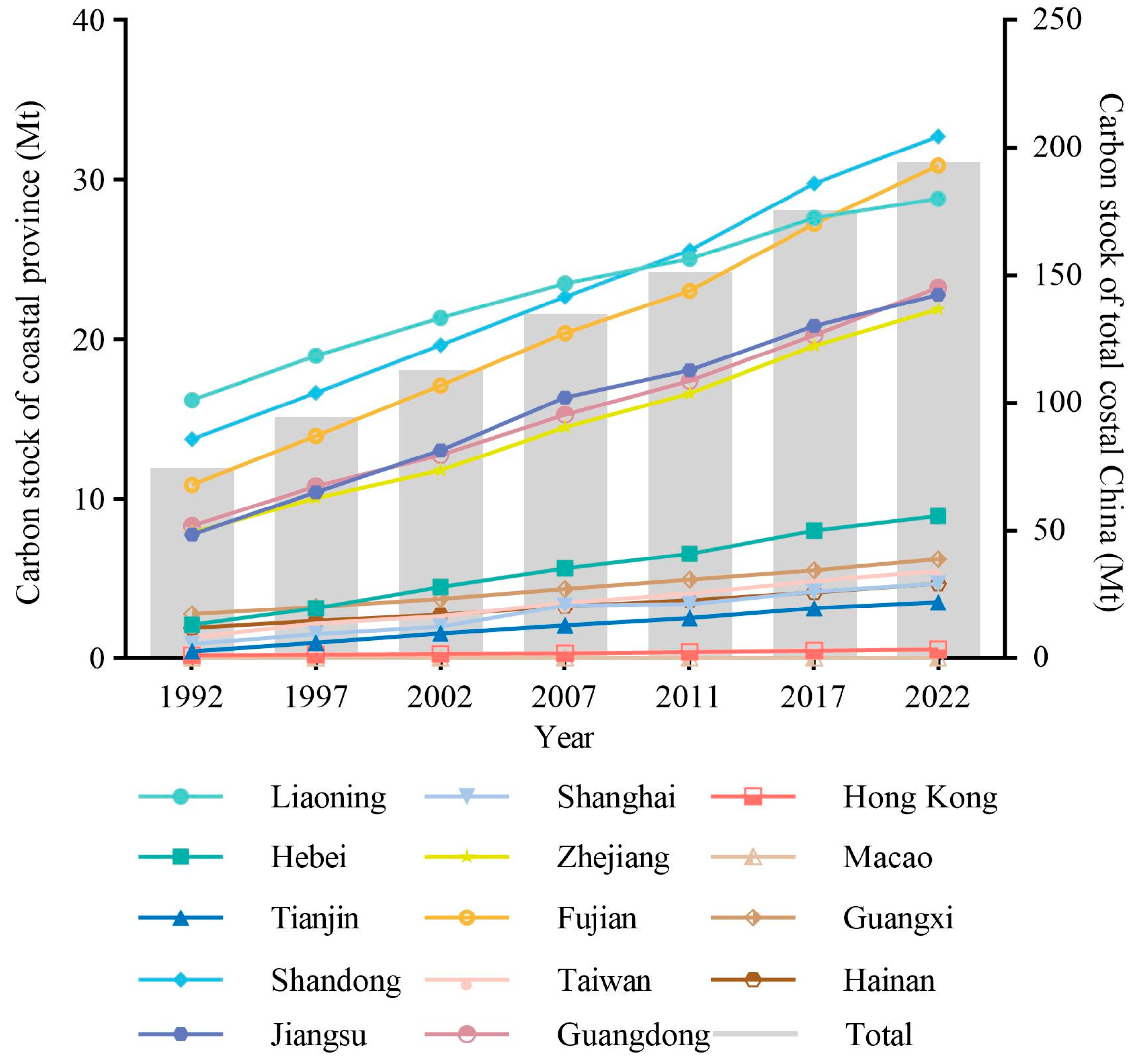
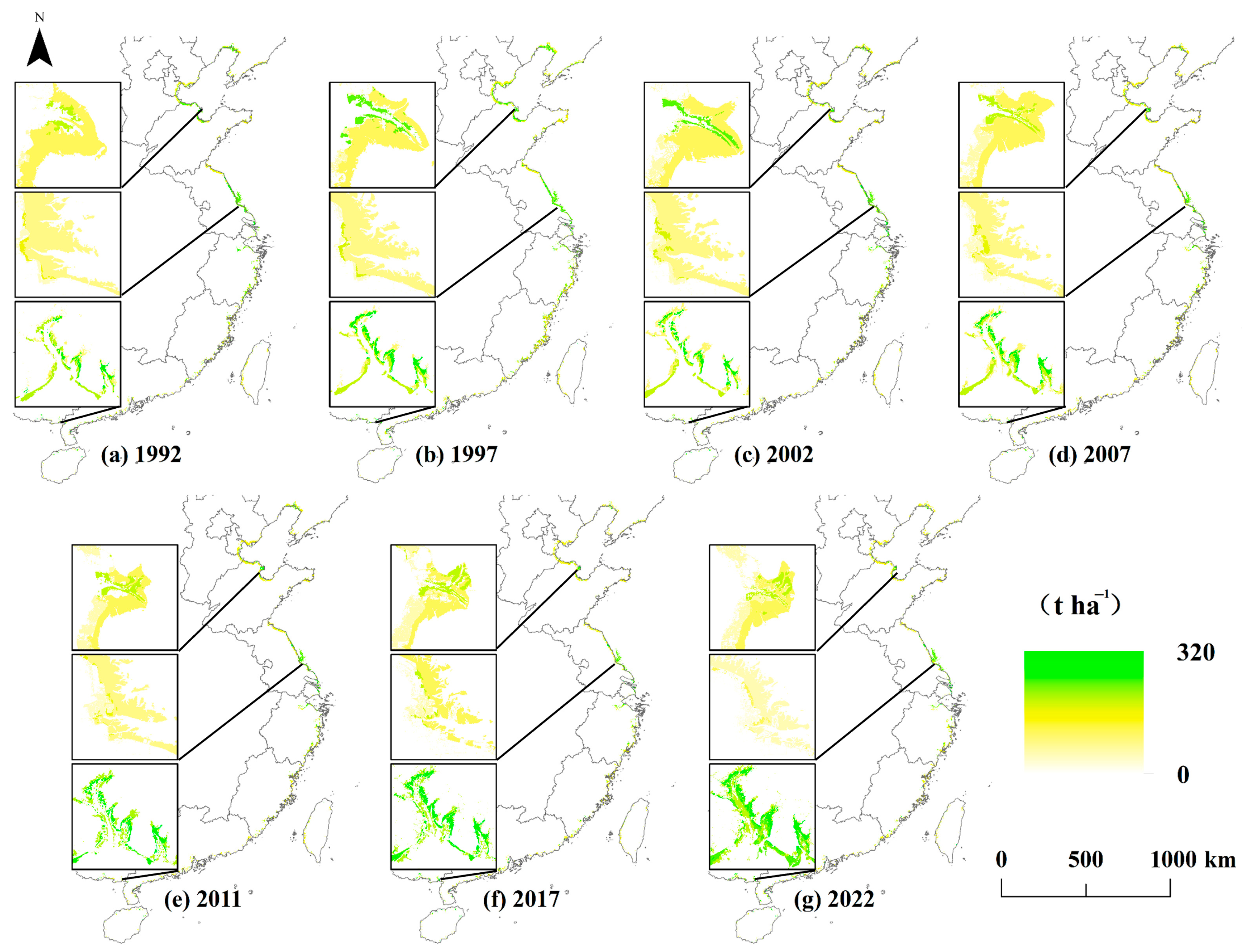
3.3. Spatiotemporal Pattern of Carbon Stock of Blue Carbon Ecosystems
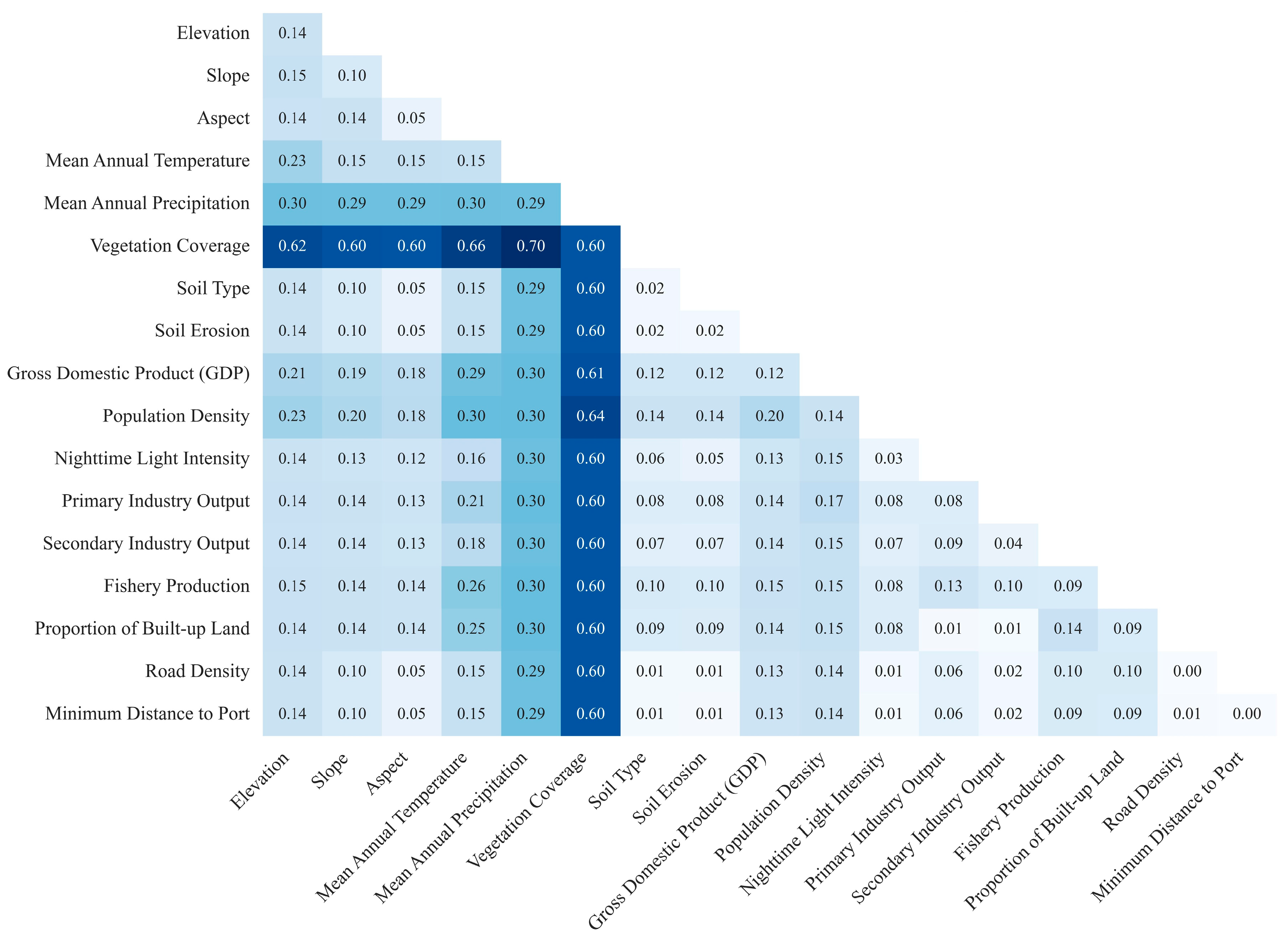
3.4. Driving Force of Carbon Stock Changes
4. Discussion
4.1. Dynamics of Blue Carbon Ecosystems and Their Carbon Stocks
4.2. Natural and Anthropogenic Drivers of Carbon Stock Change and Their Management Implications
4.3. Uncertainty and Future Research
5. Conclusions
Supplementary Materials
Author Contributions
Funding
Data Availability Statement
Conflicts of Interest
References
- Macreadie, P.I.; Anton, A.; Raven, J.A.; Beaumont, N.; Connolly, R.M.; Friess, D.A.; Kelleway, J.J.; Kennedy, H.; Kuwae, T.; Lavery, P.S.; et al. The future of Blue Carbon science. Nat. Commun. 2019, 10, 3988. [Google Scholar] [CrossRef]
- Serrano, O.; Kelleway, J.J.; Lovelock, C.; Lavery, P.S. Conservation of blue carbon ecosystems for climate change mitigation and adaptation. Coast. Wetl. 2019, 28, 965–996. [Google Scholar]
- Arkema, K.K.; Guannel, G.; Verutes, G.; Wood, S.A.; Guerry, A.; Ruckelshaus, M.; Kareiva, P.; Lacayo, M.; Silver, J.M. Coastal habitats shield people and property from sea-level rise and storms. Nat. Clim. Change 2013, 3, 913–918. [Google Scholar] [CrossRef]
- Bertram, C.; Quaas, M.; Reusch, T.B.H.; Vafeidis, A.T.; Wolff, C.; Rickels, W. The blue carbon wealth of nations. Nat. Clim. Change 2021, 11, 704–709. [Google Scholar] [CrossRef]
- Raven, J. Blue carbon: Past, present and future, with emphasis on macroalgae. Biol. Lett. 2018, 14, 20180336. [Google Scholar] [CrossRef]
- Brown, D.R.; Marotta, H.; Peixoto, R.B.; Enrich-Prast, A.; Barroso, G.C.; Soares, M.L.G.; Machado, W.; Perez, A.; Smoak, J.M.; Sanders, L.M.; et al. Hypersaline tidal flats as important “blue carbon” systems: A case study from three ecosystems. Biogeosciences 2021, 18, 2527–2538. [Google Scholar] [CrossRef]
- Zhong, C.; Li, T.; Bi, R.; Sanganyado, E.; Huang, J.; Jiang, S.; Zhang, Z.; Du, H. Systematic overview, trends and global perspectives on blue carbon: A bibliometric study (2003–2021). Ecol. Indic. 2023, 148, 110063. [Google Scholar] [CrossRef]
- Gao, G.; Beardall, J.; Jin, P.; Gao, L.; Xie, S.Y.; Gao, K.S. A review of existing and potential blue carbon contributions to climate change mitigation in the Anthropocene. J. Appl. Ecol. 2022, 59, 1686–1699. [Google Scholar] [CrossRef]
- Lovelock, C.E.; Reef, R. Variable Impacts of Climate Change on Blue Carbon. One Earth 2020, 3, 195–211. [Google Scholar] [CrossRef]
- Cuellar-Martinez, T.; Ruiz-Fernández, A.C.; Sanchez-Cabeza, J.A.; Pérez-Bernal, L.; López-Mendoza, P.G.; Carnero-Bravo, V.; Agraz-Hernández, C.M.; van Tussenbroek, B.I.; Sandoval-Gil, J.; Cardoso-Mohedano, J.G.; et al. Temporal records of organic carbon stocks and burial rates in Mexican blue carbon coastal ecosystems throughout the Anthropocene. Glob. Planet. Change 2020, 192, 103215. [Google Scholar] [CrossRef]
- Cooley, S.; Schoeman, D.; Bopp, L.; Boyd, P.; Donner, S.; Ito, S.I.; Kiessling, W.; Martinetto, P.; Ojea, E.; Racault, M.F.; et al. Oceans and Coastal Ecosystems and Their Services. In Climate Change 2022: Impacts, Adaptation and Vulnerability. Contribution of Working Group II to the Sixth Assessment Report of the Intergovernmental Panel on Climate Change; Cambridge University Press: Cambridge, UK; New York, NY, USA, 2022. [Google Scholar]
- Quevedo, J.M.D.; Uchiyama, Y.; Kohsaka, R. Progress of blue carbon research: 12 years of global trends based on content analysis of peer-reviewed and ‘gray literature’ documents. Ocean Coast. Manag. 2023, 236, 106495. [Google Scholar] [CrossRef]
- Sun, Y.Z.; Zhang, H.K.; Lin, Q.; Zhang, C.X.; He, C.; Zheng, H.P. Exploring the international research landscape of blue carbon: Based on scientometrics analysis. Ocean Coast. Manag. 2024, 252, 107106. [Google Scholar] [CrossRef]
- Arnaud, M.; Krause, S.; Norby, R.J.; Dang, T.H.; Acil, N.; Kettridge, N.; Gauci, V.; Ullah, S. Global mangrove root production, its controls and roles in the blue carbon budget of mangroves. Glob. Change Biol. 2023, 29, 3256–3270. [Google Scholar] [CrossRef]
- Song, S.; Ding, Y.; Li, W.; Meng, Y.; Zhou, J.; Gou, R.; Zhang, C.; Ye, S.; Saintilan, N.; Krauss, K.W.; et al. Mangrove reforestation provides greater blue carbon benefit than afforestation for mitigating global climate change. Nat. Commun. 2023, 14, 756. [Google Scholar] [CrossRef]
- Campbell, A.D.; Fatoyinbo, L.; Goldberg, L.; Lagomasino, D. Global hotspots of salt marsh change and carbon emissions. Nature 2022, 612, 701–706. [Google Scholar] [CrossRef] [PubMed]
- Johannessen, S.C. How can blue carbon burial in seagrass meadows increase long-term, net sequestration of carbon? A critical review. Environ. Res. Lett. 2022, 17, 093004. [Google Scholar] [CrossRef]
- Bunting, P.; Rosenqvist, A.; Hilarides, L.; Lucas, R.M.; Thomas, N.; Tadono, T.; Worthington, T.A.; Spalding, M.; Murray, N.J.; Rebelo, L.M. Global Mangrove Extent Change 1996–2020: Global Mangrove Watch Version 3.0. Remote Sens. 2022, 14, 3657. [Google Scholar] [CrossRef]
- McKenzie, L.J.; Langlois, L.A.; Roelfsema, C.M. Improving Approaches to Mapping Seagrass within the Great Barrier Reef: From Field to Spaceborne Earth Observation. Remote Sens. 2022, 14, 2604. [Google Scholar] [CrossRef]
- Chen, Z.L.; Lee, S.Y. Tidal Flats as a Significant Carbon Reservoir in Global Coastal Ecosystems. Front. Mar. Sci. 2022, 9, 900896. [Google Scholar] [CrossRef]
- Xu, C.J.; Su, G.H.; Zhao, K.S.; Wang, H.; Xu, X.Q.; Li, Z.Q.; Hu, Q.; Xu, J. Assessment of greenhouse gases emissions and intensity from Chinese marine aquaculture in the past three decades. J. Environ. Manag. 2023, 329, 117025. [Google Scholar] [CrossRef]
- Human, L.R.D.; Els, J.; Wasserman, J.; Adams, J.B. Blue carbon and nutrient stocks in salt marsh and seagrass from an urban African estuary. Sci. Total Environ. 2022, 842, 156955. [Google Scholar] [CrossRef]
- Li, P.; Liu, D.H.; Liu, C.; Li, X.X.; Liu, Z.H.; Zhu, Y.J.; Peng, B. Blue carbon development in China: Realistic foundation, internal demands, and the construction of blue carbon market trading mode. Front. Mar. Sci. 2024, 10, 1310261. [Google Scholar] [CrossRef]
- Pham, T.D.; Yokoya, N.; Bui, D.T.; Yoshino, K.; Friess, D.A. Remote Sensing Approaches for Monitoring Mangrove Species, Structure, and Biomass: Opportunities and Challenges. Remote Sens. 2019, 11, 230. [Google Scholar] [CrossRef]
- Sasmito, S.D.; Taillardat, P.; Clendenning, J.N.; Cameron, C.; Friess, D.A.; Murdiyarso, D.; Hutley, L.B. Effect of land-use and land-cover change on mangrove blue carbon: A systematic review. Glob. Change Biol. 2019, 25, 4291–4302. [Google Scholar] [CrossRef] [PubMed]
- Rogers, K.; Lymburner, L.; Salum, R.; Brooke, B.P.; Woodroffe, C.D. Mapping of mangrove extent and zonation using high and low tide composites of Landsat data. Hydrobiologia 2017, 803, 49–68. [Google Scholar] [CrossRef]
- Roy, A.D.; Arachchige, P.S.P.; Watt, M.S.; Kale, A.; Davies, M.; Heng, J.E.; Daneil, R.; Galgamuwa, G.A.P.; Moussa, L.G.; Ewane, E.B.; et al. Remote sensing-based mangrove blue carbon assessment in the Asia-Pacific: A systematic review. Sci. Total Environ. 2024, 938, 173270. [Google Scholar]
- Bajaj, M.; Sasaki, N.; Tsusaka, T.W.; Venkatappa, M.; Abe, I.; Shrestha, R.P. Assessing changes in mangrove forest cover and carbon stocks in the Lower Mekong Region using Google Earth Engine. Innov. Green Dev. 2024, 3, 100140. [Google Scholar] [CrossRef]
- Donato, D.C.; Kauffman, J.B.; Murdiyarso, D.; Kurnianto, S.; Stidham, M.; Kanninen, M. Mangroves among the most carbon-rich forests in the tropics. Nat. Geosci. 2011, 4, 293–297. [Google Scholar] [CrossRef]
- Gonzalez-Garcia, A.; Arias, M.; Garcia-Tiscar, S.; Alcorlo, P.; Santos-Martin, F. National blue carbon assessment in Spain using InVEST: Current state and future perspectives. Ecosyst. Serv. 2022, 53, 101397. [Google Scholar] [CrossRef]
- Kotagama, O.W.; Pathirage, S.; Perera, K.A.R.S.; Dahanayaka, D.D.G.L.; Miththapala, S.; Somarathne, S. Modelling predictive changes of blue carbon due to sea-level rise using InVEST model in Chilaw Lagoon, Sri Lanka. Model. Earth Syst. Environ. 2023, 9, 585–599. [Google Scholar] [CrossRef]
- Jiao, N.; Wang, H.; Xu, G.; Arico, S. Blue carbon on the rise: Challenges and opportunities. Natl. Sci. Rev. 2018, 5, 464–468. [Google Scholar] [CrossRef]
- Sasmito, S.D.; Sillanpaa, M.; Hayes, M.A.; Bachri, S.; Saragi-Sasmito, M.F.; Sidik, F.; Hanggara, B.B.; Mofu, W.Y.; Rumbiak, V.I.; Hendri; et al. Mangrove blue carbon stocks and dynamics are controlled by hydrogeomorphic settings and land-use change. Glob. Change Biol. 2020, 26, 3028–3039. [Google Scholar] [CrossRef]
- Liu, Z.; Deng, Z.; He, G.; Wang, H.L.; Zhang, X.; Lin, J.; Qi, Y.; Liang, X. Challenges and opportunities for carbon neutrality in China. Nat. Rev. Earth Environ. 2022, 3, 141–155. [Google Scholar] [CrossRef]
- Meng, W.; Feagin, R.A.; Hu, B.; He, M.; Li, H. The spatial distribution of blue carbon in the coastal wetlands of China. Estuar. Coast. Shelf Sci. 2019, 222, 13–20. [Google Scholar] [CrossRef]
- Gu, T.; Ng, C.C. Utilising coastal blue carbon (CBC) to mitigate the climate crisis: Current status and future analysis of China. Ocean Coast. Manag. 2025, 266, 107699. [Google Scholar] [CrossRef]
- Meng, Y.; Gou, R.; Bai, J.; Moreno-Mateos, D.; Davis, C.C.; Wan, L.; Song, S.; Zhang, H.; Zhu, X.; Lin, G. Spatial patterns and driving factors of carbon stocks in mangrove forests on Hainan Island, China. Glob. Ecol. Biogeogr. 2022, 31, 1692–1706. [Google Scholar] [CrossRef]
- Yu, C.; Feng, J.; Liu, K.; Wang, G.; Zhu, Y.; Cheng, H.; Guan, D. Changes of ecosystem carbon stock following the plantation of exotic mangrove Sonneratia apetala in Qi’ao Island, China. Sci. Total Environ. 2020, 717, 137142. [Google Scholar] [CrossRef] [PubMed]
- LIu, S.; Wang, L.; Zhang, J.; Ding, S.P. Opposite effect on soil organic carbon between grain and non-grain crops: Evidence from Main Grain Land, China. Agric. Ecosyst. Environ. 2025, 379, 109364. [Google Scholar] [CrossRef]
- Thurner, M.; Beer, C.; Santoro, M.; Carvalhais, N.; Wutzler, T.; Schepaschenko, D.; Shvidenko, A.; Kompter, E.; Ahrens, B.; Levick, S.R.; et al. Carbon stock and density of northern boreal and temperate forests. Glob. Ecol. Biogeogr. 2014, 23, 297–310. [Google Scholar] [CrossRef]
- Huang, Y.H.; Lee, C.L.; Chung, C.Y.; Hsiao, S.C.; Lin, H.J. Carbon budgets of multispecies seagrass beds at Dongsha Island in the South China Sea. Mar. Environ. Res. 2015, 106, 92–102. [Google Scholar] [CrossRef]
- Cai, T.; Huang, S.; Wu, J.; Zhang, Z.; Xue, C.; Chen, Y. Saltmarsh Carbon Stock Changes under Combined Effects of Vegetation Succession and Reclamation. Ecosyst. Health Sustain. 2023, 9, 0114. [Google Scholar] [CrossRef]
- Wang, F.; Sanders, C.J.; Santos, I.R.; Tang, J.; Schuerch, M.; Kirwan, M.L.; Kopp, R.E.; Zhu, K.; Li, X.; Yuan, J.; et al. Global blue carbon accumulation in tidal wetlands increases with climate change. Natl. Sci. Rev. 2021, 8, nwaa296. [Google Scholar] [CrossRef]
- Sun, X.; Filgueira, R.; Sun, Y.; Han, M.; Tang, Q.; Sun, Y. Intensive oyster farming enhances carbon storage in sediments over decades. Commun. Earth Environ. 2025, 6, 383. [Google Scholar] [CrossRef]
- Kwan, V.; Fong, J.; Ng, C.S.L.; Huang, D. Temporal and spatial dynamics of tropical macroalgal contributions to blue carbon. Sci. Total Environ. 2022, 828, 154369. [Google Scholar] [CrossRef]
- Krause-Jensen, D.; Duarte, C.M. Substantial role of macroalgae in marine carbon sequestration. Nat. Geosci. 2016, 9, 737–742. [Google Scholar] [CrossRef]
- Feng, J.C.; Sun, L.; Yan, J. Carbon sequestration via shellfish farming: A potential negative emissions technology. Renew. Sustain. Energy Rev. 2023, 171, 113018. [Google Scholar] [CrossRef]
- Gorelick, N.; Hancher, M.; Dixon, M.; Ilyushchenko, S.; Thau, D.; Moore, R. Google Earth Engine: Planetary-scale geospatial analysis for everyone. Remote Sens. Environ. 2017, 202, 18–27. [Google Scholar] [CrossRef]
- Chen, C.; Yang, X.B.; Jiang, S.H.; Liu, Z.S. Mapping and spatiotemporal dynamics of land-use and land-cover change based on the Google Earth Engine cloud platform from Landsat imagery: A case study of Zhoushan Island, China. Heliyon 2023, 9, e19654. [Google Scholar] [CrossRef] [PubMed]
- Campillo-Tamarit, N.; Molner, J.V.; Soria, J.M. Remote Sensing Tools for Monitoring Marine Phanerogams: A Review of Sentinel and Landsat Applications. J. Mar. Sci. Eng. 2025, 13, 292. [Google Scholar] [CrossRef]
- Unsworth, R.K.F.; Cullen-Unsworth, L.C.; Jones, B.L.H.; Lilley, R.J. The planetary role of seagrass conservation. Science 2022, 377, 609–613. [Google Scholar] [CrossRef]
- Wang, F.; Liu, J.; Qin, G.; Zhang, J.; Zhou, J.; Wu, J.; Ren, H. Coastal blue carbon in China as a nature-based solution toward carbon neutrality. Innovation 2023, 4, 100481. [Google Scholar] [CrossRef]
- Pinkeaw, S.; Boonrat, P.; Koedsin, W.; Huete, A. Semi-automated mangrove mapping at National-Scale using Sentinel-2, Sentinel-1, and SRTM data with Google Earth Engine: A case study in Thailand. Egypt. J. Remote Sens. Space Sci. 2024, 27, 555–564. [Google Scholar] [CrossRef]
- Zhang, Q.; Zhang, G.L.; Xiao, X.M.; Zhang, Y.; You, N.S.; Di, Y.Y.; Yang, T.; He, Y.L.; Dong, J.W. Unraveling the spatial-temporal patterns of typhoon impacts on maize during the milk stage in Northeast China in 2020. Eur. J. Agron. 2024, 156, 127169. [Google Scholar] [CrossRef]
- Amindin, A.; Siamian, N.; Kariminejad, N.; Clague, J.J.; Pourghasemi, H.R. An integrated GEE and machine learning framework for detecting ecological stability under land use/land cover changes. Glob. Ecol. Conserv. 2024, 53, e03010. [Google Scholar] [CrossRef]
- Aji, M.A.P.; Kamal, M.; Farda, N.M. Mangrove species mapping through phenological analysis using random forest algorithm on Google Earth Engine. Remote Sens. Appl. Soc. Environ. 2023, 30, 100978. [Google Scholar] [CrossRef]
- Bera, D.; Das Chatterjee, N.; Bera, S.; Ghosh, S.; Dinda, S. Comparative performance of Sentinel-2 MSI and Landsat-8 OLI data in canopy cover prediction using Random Forest model: Comparing model performance and tuning parameters. Adv. Space Res. 2023, 71, 4691–4709. [Google Scholar] [CrossRef]
- Nelson, E.; Sander, H.; Hawthorne, P.; Conte, M.; Ennaanay, D.; Wolny, S.; Manson, S.; Polasky, S. Projecting Global Land-Use Change and Its Effect on Ecosystem Service Provision and Biodiversity with Simple Models. PLoS ONE 2010, 5, e14327. [Google Scholar] [CrossRef]
- Li, Y.; Qiu, J.H.; Li, Z.; Li, Y.F. Assessment of Blue Carbon Storage Loss in Coastal Wetlands under Rapid Reclamation. Sustainability 2018, 10, 2818. [Google Scholar] [CrossRef]
- Yuan, Y.Q.; Li, X.Z.; Jiang, J.Y.; Xue, L.M.; Craft, C.B. Distribution of organic carbon storage in different salt-marsh plant communities: A case study at the Yangtze Estuary. Estuar. Coast. Shelf Sci. 2020, 243, 106900. [Google Scholar] [CrossRef]
- Shi, X.; Wu, L.; Zheng, Y.Q.; Zhang, X.; Wang, Y.J.; Chen, Q.; Sun, Z.Y.; Nie, T.Z. Dynamic Estimation of Mangrove Carbon Storage in Hainan Island Based on the InVEST-PLUS Model. Forests 2024, 15, 750. [Google Scholar] [CrossRef]
- Ke, L.; Lei, N.; Zhang, S.; Yin, C.; Lu, Y.; Wang, L.; Wang, Q. Estimation of blue carbon stock in the Liaohe Estuary wetland based on soil thickness and multi-scenario modeling. Ecol. Indic. 2025, 171, 113201. [Google Scholar] [CrossRef]
- Lai, Q.; Jia, M.; He, F.; Zhang, A.; Pei, D.; Yu, M. Current and Future Potential of Shellfish and Algae Mariculture Carbon Sinks in China. Int. J. Environ. Res. Public Health 2022, 19, 8873. [Google Scholar] [CrossRef] [PubMed]
- Wang, J.F.; Hu, Y. Environmental health risk detection with GeogDetector. Environ. Modell. Softw. 2012, 33, 114–115. [Google Scholar] [CrossRef]
- Huang, X.D.; Liu, X.Q.; Wang, Y. Spatio-Temporal Variations and Drivers of Carbon Storage in the Tibetan Plateau Under SSP-RCP Scenarios Based on the PLUS-InVEST-GeoDetector Model. Sustainability 2024, 16, 5711. [Google Scholar] [CrossRef]
- Li, Y.T.; Zhu, C.M.; Yang, R.M.; Xu, L.; Zhang, X. Spatial patterns of soil organic carbon stocks and its controls in Chinese grassland ecosystems. Geoderma 2024, 448, 116970. [Google Scholar] [CrossRef]
- Wang, Y.; Wang, M.; Zhang, J.R.; Wu, Y.M.; Zhou, Y. Assessment of carbon stocks and influencing factors in terrestrial ecosystems based on surface area. iScience 2024, 27, 111431. [Google Scholar] [CrossRef]
- Cai, J.H.; Chi, H.; Lu, N.; Bian, J.; Chen, H.Q.; Yu, J.K.; Yang, S.Q. Analysis of Spatiotemporal Predictions and Drivers of Carbon Storage in the Pearl River Delta Urban Agglomeration via the PLUS-InVEST-GeoDetector Model. Energies 2024, 17, 5093. [Google Scholar] [CrossRef]
- Wang, J.F.; Zhang, T.L.; Fu, B.J. A measure of spatial stratified heterogeneity. Ecol. Indic. 2016, 67, 250–256. [Google Scholar] [CrossRef]
- Wang, J.F.; Li, X.H.; Christakos, G.; Liao, Y.L.; Zhang, T.; Gu, X.; Zheng, X.Y. Geographical Detectors-Based Health Risk Assessment and its Application in the Neural Tube Defects Study of the Heshun Region, China. Int. J. Geogr. Inf. Sci. 2010, 24, 107–127. [Google Scholar] [CrossRef]
- Wang, J.; Xu, X. Geodetector: Principle and prospective. Acta Geogr. Sin. 2017, 72, 116–134. (In Chinese) [Google Scholar]
- Richards, D.R.; Thompson, B.S.; Wijedasa, L. Quantifying net loss of global mangrove carbon stocks from 20 years of land cover change. Nat. Commun. 2020, 11, 4260. [Google Scholar] [CrossRef]
- Wang, X.X.; Xiao, X.M.; Zou, Z.H.; Chen, B.Q.; Ma, J.; Dong, J.W.; Doughty, R.B.; Zhong, Q.Y.; Qin, Y.W.; Dai, S.Q.; et al. Tracking annual changes of coastal tidal flats in China during 1986–2016 through analyses of Landsat images with Google Earth Engine. Remote Sens. Environ. 2020, 238, 110987. [Google Scholar] [CrossRef] [PubMed]
- Guo, S.M.; Nie, H.T. Estimation of Mariculture Carbon Sinks in China and Its Influencing Factors. J. Mar. Sci. Eng. 2024, 12, 724. [Google Scholar] [CrossRef]
- Lu, W.Z.; Xiao, J.F.; Gao, H.Q.; Jia, Q.Y.; Li, Z.J.; Liang, J.; Xing, Q.H.; Mao, D.H.; Li, H.; Chu, X.J.; et al. Carbon fluxes of China’s coastal wetlands and impacts of reclamation and restoration. Glob. Change Biol. 2024, 30, e17280. [Google Scholar] [CrossRef] [PubMed]
- Tang, Z.X.; Wang, D.; Tian, X.P.; Bi, X.L.; Zhou, Z.X.; Luo, F.B.; Ning, R.R.; Li, J.R. Exploring the factors influencing the carbon sink function of coastal wetlands in the Yellow River Delta. Sci. Rep. 2024, 14, 28938. [Google Scholar] [CrossRef]
- Xie, Z.X.; Li, H.A.; Yuan, Y.; Hu, W.; Luo, G.; Huang, L.T.; Chen, M.; Wu, W.M.; Yan, G.L.; Sun, X. The spatial patterns and driving mechanisms of blue carbon ‘loss’ and ‘gain’ in a typical mangrove ecosystem: A case study of Beihai, Guangxi Province of China. Sci. Total Environ. 2023, 905, 167241. [Google Scholar] [CrossRef]
- Alongi, D.M. Impacts of Climate Change on Blue Carbon Stocks and Fluxes in Mangrove Forests. Forests 2022, 13, 149. [Google Scholar] [CrossRef]
- Saintilan, N.; Wilson, N.; Rogers, K. Mangrove expansion and salt-marsh decline at the mangrove–salt-marsh interface in south-east Australia. Glob. Change Biol. 2020, 26, 3058–3071. [Google Scholar]
- Simard, M.; Fatoyinbo, L.; Smetanka, C.; Rivera-Monroy, V.H.; Castañeda-Moya, E.; Thomas, N.; Van der Stocken, T. Mangrove canopy height globally related to precipitation, temperature and cyclone frequency. Nat. Geosci. 2019, 12, 40–45. [Google Scholar] [CrossRef]
- Yao, Y.L.; Wang, C.Z. Subsurface Marine Heatwaves in the South China Sea. J. Geophys. Res. Ocean. 2024, 129, e2024JC021356. [Google Scholar] [CrossRef]
- Chen, Y.; Li, G.; Cui, L.; Li, L.; He, L.; Ma, P. The effects of tidal flat reclamation on the stability of the coastal area in the Jiangsu Province, China, from the perspective of landscape structure. Land 2022, 11, 421. [Google Scholar] [CrossRef]
- Friess, D.A.; Rogers, K.; Lovelock, C.E.; Krauss, K.W.; Hamilton, S.E.; Lee, S.Y.; Lucas, R.; Primavera, J.; Rajkaran, A.; Shi, S.H. The State of the World’s Mangrove Forests: Past, Present, and Future. Annu. Rev. Environ. Resour. 2019, 44, 89–115. [Google Scholar] [CrossRef]
- Billah, M.M.; Bhuiyan, M.K.A.; Islam, M.A.; Das, J.; Hoque, A.T.M.R. Salt marsh restoration: An overview of techniques and success indicators. Environ. Sci. Pollut. Res. 2022, 29, 15347–15363. [Google Scholar] [CrossRef] [PubMed]
- Fu, C.C.; Li, Y.; Zeng, L.; Zhang, H.B.; Tu, C.; Zhou, Q.; Xiong, K.X.; Wu, J.P.; Duarte, C.M.; Christie, P.; et al. Stocks and losses of soil organic carbon from Chinese vegetated coastal habitats. Glob. Change Biol. 2021, 27, 202–214. [Google Scholar] [CrossRef] [PubMed]
- Lu, Y.; Chen, J.; Gao, G.; An, A.; Feng, J.; Liu, Z. Estimation of carbon stock in the reed wetland of Weishan county in China based on Sentinel satellite series. Carbon Res. 2025, 4, 29. [Google Scholar] [CrossRef]
- Tikuye, B.G.; Tefera, G.W.; Gurau, S.; Ray, R.L. Assessing carbon stock and sequestration potential under land use and land cover dynamics in the Upper Blue Nile River Basin, Ethiopia. Carbon Manag. 2025, 16, 2479516. [Google Scholar] [CrossRef]
- Mukhopadhyay, A.; Hati, J.P.; Acharyya, R.; Pal, I.; Tuladhar, N.; Habel, M. Global trends in using the InVEST model suite and related research: A systematic review. Ecohydrol. Hydrobiol. 2025, 25, 389–405. [Google Scholar] [CrossRef]
- Chen, J.; An, A.H.; Gao, G.P. A substantial reduction of total and group-specific population risk to compound heat and drought events in China through achieving carbon neutrality. J. Clean. Prod. 2025, 489, 144694. [Google Scholar] [CrossRef]
- Griffith, D.A.; Peres-Neto, P.R. Spatial modeling in ecology: The flexibility of eigenfunction spatial analyses. Ecology 2006, 87, 2603–2613. [Google Scholar] [CrossRef]
- Latimer, A.M.; Wu, S.S.; Gelfand, A.E.; Silander, J.A. Building statistical models to analyze species distributions. Ecol. Appl. 2006, 16, 33–50. [Google Scholar] [CrossRef]

| Year | Satellite | Sensor | Analysis-Ready Data (ARD) Collection | Wavelength/μm | Total Number of Images |
|---|---|---|---|---|---|
| 1992 | Landsat 5 | TM | LANDSAT/LT05/C02/T1_L2 | Blue: 0.45–0.52 Green: 0.52–0.60 Red: 0.63–0.69 NIR: 0.77–0.90 SWIR1: 1.55–1.75 SWIR2: 2.08–2.35 | 940 |
| 1997 | Landsat 5 | TM | LANDSAT/LT05/C02/T1_L2 | 898 | |
| 2002 | Landsat 5 | TM | LANDSAT/LT05/C02/T1_L2 | 740 | |
| 2007 | Landsat 5 | TM | LANDSAT/LT05/C02/T1_L2 | 749 | |
| 2011 | Landsat 5 | TM | LANDSAT/LT05/C02/T1_L2 | 621 | |
| 2017 | Landsat 8 | OLI | LANDSAT/LC08/C02/T1_L2 | Blue: 0.45–0.51 Green: 0.53–0.59 Red: 0.64–0.67 NIR: 0.85–0.88 SWIR1: 1.57–1.65 SWIR2: 2.11–2.29 | 1145 |
| 2022 | Landsat 8 | OLI | LANDSAT/LC08/C02/T1_L2 | 1104 |
| Province | Carbon Density (t ha −1) | ||
|---|---|---|---|
| Plant | Soil | Litter | |
| Zhejiang | 104.73 ± 137.93 | 225.29 ± 133.13 | 1.40 ± 2.16 |
| Fujian | 81.88 ± 94.63 | 149.13 ± 92.07 | 3.93 ± 2.18 |
| Taiwan | 173.45 ± 116.43 | 267.50 ± 93.68 | 2.08 ± 1.82 |
| Guangdong | 125.90 | 147.38 | 5.81 |
| Hong Kong | 173.45 | 268.30 | 2.08 |
| Macao | 173.45 | 283.24 | 2.08 |
| Guangxi | 132.53 | 204.33 | 2.08 |
| Hainan | 115.11 | 201.42 | 2.08 |
| The national average | 135.06 ± 32.90 | 218.32 ± 49.35 | 2.69 ± 1.36 |
| Province | Carbon Density (t ha −1) | ||
|---|---|---|---|
| Plant | Soil | Litter | |
| Liaoning | 13.34 ± 10.90 | 101.40 ± 71.25 | 5.01 |
| Hebei | 16.28 ± 2.49 | 81.40 ± 46.60 | 5.01 |
| Tianjin | 16.28 ± 2.49 | 82.20 ± 40.17 | 5.01 |
| Shandong | 11.71 ± 8.16 | 56.95 ± 43.73 | 2.75 ± 3.19 |
| Jiangsu | 16.75 ± 10.84 | 72.04 ± 81.05 | 7.00 |
| Shanghai | 12.59 ± 11.38 | 70.71 ± 63.49 | 3.51 ± 4.94 |
| Zhejiang | 9.87 ± 7.20 | 61.06 ± 77.52 | 4.80 |
| Fujian | 16.50 ± 5.40 | 101.39 ± 42.32 | 4.80 |
| Taiwan | 19.77 ± 1.41 | 173.04 ± 54.69 | 4.80 |
| Guangdong | 19.77 ± 1.41 | 140.84 ± 66.84 | 4.80 |
| Hong Kong | 19.77 ± 1.41 | 132.92 ± 79.52 | 4.80 |
| Macao | 19.77 ± 1.41 | 132.92 ± 79.52 | 4.80 |
| Guangxi | 18.26 ± 2.80 | 100.72 ± 89.33 | 4.80 |
| Hainan | 16.34 ± 6.01 | 122.03 ± 96.44 | 4.80 |
| The national average | 16.21 ± 3.25 | 102.12 ± 34.28 | 4.76 ± 0.91 |
| Type | GEE Image Example | Description |
|---|---|---|
| Tidal flats | 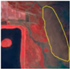 | Located at the junction of land and water, the tone is dark, uniform texture, dark grayish brown. |
| Salt marshes | 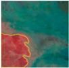 | Adjacent to the tidal flats, the surface of vegetation, irregular shape, clear boundary, smooth texture, dark red. |
| Mangroves | 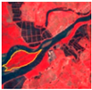 | Adjacent to the tidal flats, the surface of vegetation, irregular shape, clear boundary, smooth texture, bright red. |
| Mariculture | 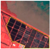 | Located in coastal wetlands, bay, and nearshore seawater, concentrated distribution, regular shape, clear boundary, and dark gray. |
| Feature Types | Feature Variables | Formula and Description |
|---|---|---|
| Spectral index | Normalized Difference Vegetation Index (NDVI) | |
| Normalized Difference Built-up Index (NDBI) | ||
| Enhanced Vegetation Index (EVI) | ||
| Soil-Adjusted Vegetation Index (SAVI) | ||
| Land Surface Water Index (LSWI) | ||
| Modified Normalized Difference Water Index (mNDWI) | ||
| Spectral band | Blue, green, red, near-infrared, short-wave infrared (SWIR1, SWIR2) | |
| Topographic features | Slope | |
| Elevation | ||
| Texture features | Brightness | |
| Greenness | ||
| Wetness | ||
| Basis for Judgment | Interactions |
|---|---|
| q(A∩B) < Minimum(q(A), q(B)) | Weaken, nonlinear |
| Minimum(q(A), q(B)) < q(A∩B) < Maximum(q(A), q(B)) | Weaken, univariate |
| q(A∩B) = q(A) + q(B) | Independent |
| q(A∩B) > Maximum (q(A), q(B)) | Enhance, bivariate |
| q(A∩B) > q(A) + q(B) | Enhance, nonlinear |
| Parameter | All Variables OA | Top 10 Variables OA | Top 5 Variables OA | All Variables Kappa | Top 10 Variables Kappa | Top 5 Variables Kappa |
|---|---|---|---|---|---|---|
| ntree | ||||||
| 100 | 92.33% | 88.33% | 84.78% | 0.91 | 0.86 | 0.83 |
| 200 | 92.59% | 88.00% | 84.78% | 0.91 | 0.86 | 0.83 |
| 300 | 92.71% | 88.67% | 84.92% | 0.91 | 0.87 | 0.84 |
| 400 | 92.74% | 89.00% | 84.97% | 0.91 | 0.87 | 0.84 |
| 500 | 92.77% | 89.00% | 84.89% | 0.92 | 0.87 | 0.84 |
| mtry | ||||||
| 3 | 92.72% | 88.20% | 84.98% | 0.91 | 0.86 | 0.84 |
| 4 | 92.60% | 88.60% | 84.91% | 0.91 | 0.87 | 0.84 |
| 5 | 92.57% | 89.00% | 84.72% | 0.91 | 0.87 | 0.83 |
Disclaimer/Publisher’s Note: The statements, opinions and data contained in all publications are solely those of the individual author(s) and contributor(s) and not of MDPI and/or the editor(s). MDPI and/or the editor(s) disclaim responsibility for any injury to people or property resulting from any ideas, methods, instructions or products referred to in the content. |
© 2025 by the authors. Licensee MDPI, Basel, Switzerland. This article is an open access article distributed under the terms and conditions of the Creative Commons Attribution (CC BY) license (https://creativecommons.org/licenses/by/4.0/).
Share and Cite
Chen, J.; Lu, Y.; Liu, F.; Gao, G.; Xie, M. Remote Sensing Evidence of Blue Carbon Stock Increase and Attribution of Its Drivers in Coastal China. Remote Sens. 2025, 17, 2559. https://doi.org/10.3390/rs17152559
Chen J, Lu Y, Liu F, Gao G, Xie M. Remote Sensing Evidence of Blue Carbon Stock Increase and Attribution of Its Drivers in Coastal China. Remote Sensing. 2025; 17(15):2559. https://doi.org/10.3390/rs17152559
Chicago/Turabian StyleChen, Jie, Yiming Lu, Fangyuan Liu, Guoping Gao, and Mengyan Xie. 2025. "Remote Sensing Evidence of Blue Carbon Stock Increase and Attribution of Its Drivers in Coastal China" Remote Sensing 17, no. 15: 2559. https://doi.org/10.3390/rs17152559
APA StyleChen, J., Lu, Y., Liu, F., Gao, G., & Xie, M. (2025). Remote Sensing Evidence of Blue Carbon Stock Increase and Attribution of Its Drivers in Coastal China. Remote Sensing, 17(15), 2559. https://doi.org/10.3390/rs17152559