A Minimal Solution for Binocular Camera Relative Pose Estimation Based on the Gravity Prior

Abstract

High-precision positioning is the foundation for the functionality of various intelligent agents. In complex environments, such as urban canyons, relative pose estimation using cameras is a crucial step in high-precision positioning. To take advantage of the ability of an inertial measurement unit (IMU) to provide relatively accurate gravity prior information over a short period, we propose a minimal solution method for the relative pose estimation of a stereo camera system assisted by the IMU. We rigidly connect the IMU to the camera system and use it to obtain the rotation matrices in the roll and pitch directions for the entire system, thereby reducing the minimum number of corresponding points required for relative pose estimation. In contrast to classic pose-estimation algorithms, our method can also calculate the camera focal length, which greatly expands its applicability. We constructed a simulated dataset and used it to compare and analyze the numerical stability of the proposed method and the impact of different levels of noise on algorithm performance. We also collected real-scene data using a drone and validated the proposed algorithm. The results on real data reveal that our method exhibits smaller errors in calculating the relative pose of the camera system compared with two classic reference algorithms. It achieves higher precision and stability and can provide a comparatively accurate camera focal length.

1. Introduction

With the continuous advancement of technology, an increasing number of intelligent agents have been integrated into people’s lives, such as intelligent vehicles, drones, and household robots. Highly precise and reliable continuous pose estimation is an essential prerequisite for intelligent agents to fulfill their designated functions. The most mature approach currently available is based on the Global Navigation Satellite System (GNSS) and inertial navigation system (INS) [1,2]. However, because intelligent agents are often used in urban canyons, indoor environments, and other similar settings, GNSS signals are frequently interrupted for extended periods. Moreover, the positioning accuracy of an INS tends to deteriorate rapidly over time. Therefore, it is imperative to explore new methods for pose estimation.

Because of the advantages of cameras, such as their autonomy, passivity, richness of information, high data acquisition frequency, and low cost, camera-based visual navigation methods have been continuously developed in recent years, with a large number of solutions emerging for the high-precision positioning and orientation of intelligent agents [3,4,5,6]. Vision navigation can be roughly divided into monocular and binocular camera systems. In practical application scenarios, monocular cameras cannot estimate the depth of the target or the scale of displacement, and hence binocular cameras have a broader range of applications. In addition, binocular camera systems can provide a larger field of view, acquire richer information, and have better robustness and accuracy. Therefore, it is necessary to study pose estimation methods based on binocular cameras [7,8]. The biggest difference between binocular camera systems and monocular cameras is that all the rays in a binocular camera system do not focus on a single point. Therefore, the imaging of binocular camera systems is usually modeled using a generalized model [9].

The Plücker line is typically employed to characterize the generalized camera model, which is a 6 × 1 column vector. The first three rows represent the direction of the line, whereas the last three rows denote its moment [9]. For a binocular camera system with known intrinsic parameters, when the cameras are rigidly connected, the relative pose can be computed using six-point correspondences. Commonly used cameras have square pixels with a fixed aspect ratio, and the principal point is located near the center of the image. Moreover, the distortion of a single camera is relatively weak. Therefore, the most crucial aspect of estimating intrinsic parameters is to determine the camera’s focal length [10,11]. In practical applications, errors are inevitably introduced during the feature point extraction and matching process. Thus, the random sample consensus (RANSAC) algorithm is often employed for joint solutions [12]. Since the number of iterations of RANSAC increases rapidly with increases in the minimum sample size, using a smaller number of minimum matching points enhances the efficiency and robustness of the solution. Consequently, it is essential to investigate the minimal configuration solution for the relative pose estimation problem of multi-camera systems. Because an IMU can provide relatively accurate gravity prior information, namely the pitch and roll angles, rigidly connecting an IMU to a multi-camera system enables us to provide partial rotation angles of the system, thereby reducing the minimum number of matching points required for relative pose estimation.

In this research, we propose a method for estimating the relative pose of a multi-camera system under the condition of unknown camera focal lengths. Our main contributions are as follows:

• We propose a minimal solution for relative pose estimation by leveraging the gravity prior information obtained from the IMU, to calculate the camera focal length, relative rotation matrix, and relative translation vector.
• We constructed both simulated and real datasets and conducted a detailed analysis and summary of the proposed method and two classic methods on these datasets, thereby verifying the reliability of our approach.

The sections of this paper are arranged as follows: First, in Section 2, we summarize and discuss the progress and limitations of relative pose estimation algorithms for multi-camera systems. Section 3 briefly introduces the generalized camera model and proposes a minimal solution method for calculating the camera focal length, rotation matrix, and translation vector using gravity prior information. In Section 4, we introduce the simulated and real datasets we constructed and compare and analyze our method with existing classic methods to verify its reliability. The conclusions are presented in Section 5.

2. Related Work

Because multi-camera systems can calculate information, such as target depth and the scale of displacement, the industry currently prefers multi-camera systems over single-camera systems, especially for devices that require autonomous control, such as drones.

In contrast to monocular camera systems, multi-camera systems do not have a single projection center, and therefore, their camera model does not conform to the pinhole model. Pless first introduced the concept of a Plücker line and derived the model for a generalized camera based on this concept, laying the foundation for many subsequent scholars to describe multi-camera systems [9]. In addition, Pless conducted a structural analysis of the motion algorithm for multi-camera system models. Frahm et al. assumed that the cameras in a multi-camera system are rigidly connected and introduced the estimation of the rigid motion of the multi-camera system itself, proposing a method for estimating the pose of a multi-camera system with known intrinsic parameters [13]. Li et al. proposed a linear solution that requires 17 pairs of matching points [14]. However, the high number of required matching point pairs leads to a very high number of iterations in RANSAC, resulting in low computational efficiency and sensitivity to noise. Stewenius et al. proposed a minimal configuration solution method based on Gröbner bases [15]. This method requires at least six pairs of matching points and computes 64 candidate solutions by solving a 64 × 64 matrix. However, because of its high computational complexity, real-time operation is not feasible. Clipp et al. proposed a method for calculating the relative pose of a multi-camera system using six points [16]. In this method, five matching point pairs are selected in one camera to calculate the relative pose, excluding the displacement scale. Then, one point pair is selected from another camera to calculate the scale information. This allows the scale to be calculated without overlapping fields of view.

To minimize the number of matching point pairs required for estimating the relative pose of a multi-camera system, commonly used methods include incorporating motion constraints and using the local information of feature points. For multi-camera systems undergoing planar motion, Stewenius et al. investigated three scenarios: (1) eight points in an image captured by one camera; (2) three points in views captured by two cameras; and (3) two points in views captured by two cameras [17]. Ventura et al. proposed a method for approximating the rotation matrix to the first order when the motion of the camera system changes little between adjacent moments [18]. This approximation simplifies the solution process and is suitable for estimating the motion of cameras with high frame rates. However, it requires a 20th-order polynomial to be solved, which is computationally complex and susceptible to noise. Wang et al. proposed an iterative weighted optimization scheme based on a planar motion model that minimizes the geometrical errors without relying on optimization variables associated with 3D points [7]. Kneip et al. proposed a nonlinear optimization algorithm based on an eigenvalue minimization strategy that requires at least seven pairs of matching points to ensure convergence to a unique solution [19]. This algorithm is faster than previous algorithms but is prone to falling into local minima. Lim et al. decoupled the rotation matrix and translation vector of a multi-camera system using point correspondences in a wide field-of-view camera, allowing them to be computed separately in lower dimensions [20]. They also proposed a new structure-from-motion algorithm to reduce computational complexity. Zhao et al. categorized the problem into seven cases according to the configuration of the multi-camera system and provided solvers for each case [21].

In addition to the cameras used in the aforementioned methods, information from other sensors can also be incorporated. Current drones, intelligent vehicles, and other intelligent devices are commonly also equipped with sensors other than cameras. Using the information provided by these multiple sensors can effectively simplify the calculation of relative poses [22]. An IMU has the advantages of high data frequency and high measurement accuracy over a short period of time, which is why many researchers have studied the use of IMU data to assist the calculation of camera relative pose [23,24,25]. If the IMU is rigidly connected to the camera system, the calibration relationship between them is well defined and known. In this configuration, the IMU can provide two rotational angles: pitch and roll. As a result, the degrees of freedom of the rotation matrix for a multi-camera system are reduced from three to one. Lee et al. proposed a method for solving polynomials based on implicit function theory and provided minimal 4-point and linear 8-point algorithms for calculating the relative pose of multi-camera systems [26]. Liu et al. focused on the relative pose problem of autonomous vehicles operating at high speeds and in complex environments. By leveraging specific prior knowledge from autonomous driving scenarios, they proposed an efficient 4-point algorithm for estimating the relative pose of multi-camera systems [27]. This algorithm obtains analytical solutions by solving polynomial equations. Since the polynomial equations constructed by this method have a lower order than those in Lee et al.’s method, it achieves a higher computational efficiency while maintaining a similar accuracy.

Existing research primarily focuses on scenarios in which the intrinsic parameters of the cameras are predetermined. However, in practical applications, there are often cases where the intrinsic parameters, especially the focal length, are unknown. To address this issue, we propose a method that simultaneously estimates the camera focal length and relative pose. Our proposed method also employs an IMU for assistance by rigidly connecting it to the camera and calibrating its relationship. Therefore, we can obtain partial rotation angles of the binocular camera system, reducing the degrees of freedom of the rotation matrix when calculating the relative pose of the cameras. This decreases the required minimum number of matching point pairs. Unlike previous algorithms that only estimate the relative pose, our method simultaneously calculates the focal lengths of the cameras. This means that our algorithm can be used when the focal length of the camera has not been calibrated, significantly expanding its range of application scenarios

3. Materials and Methods

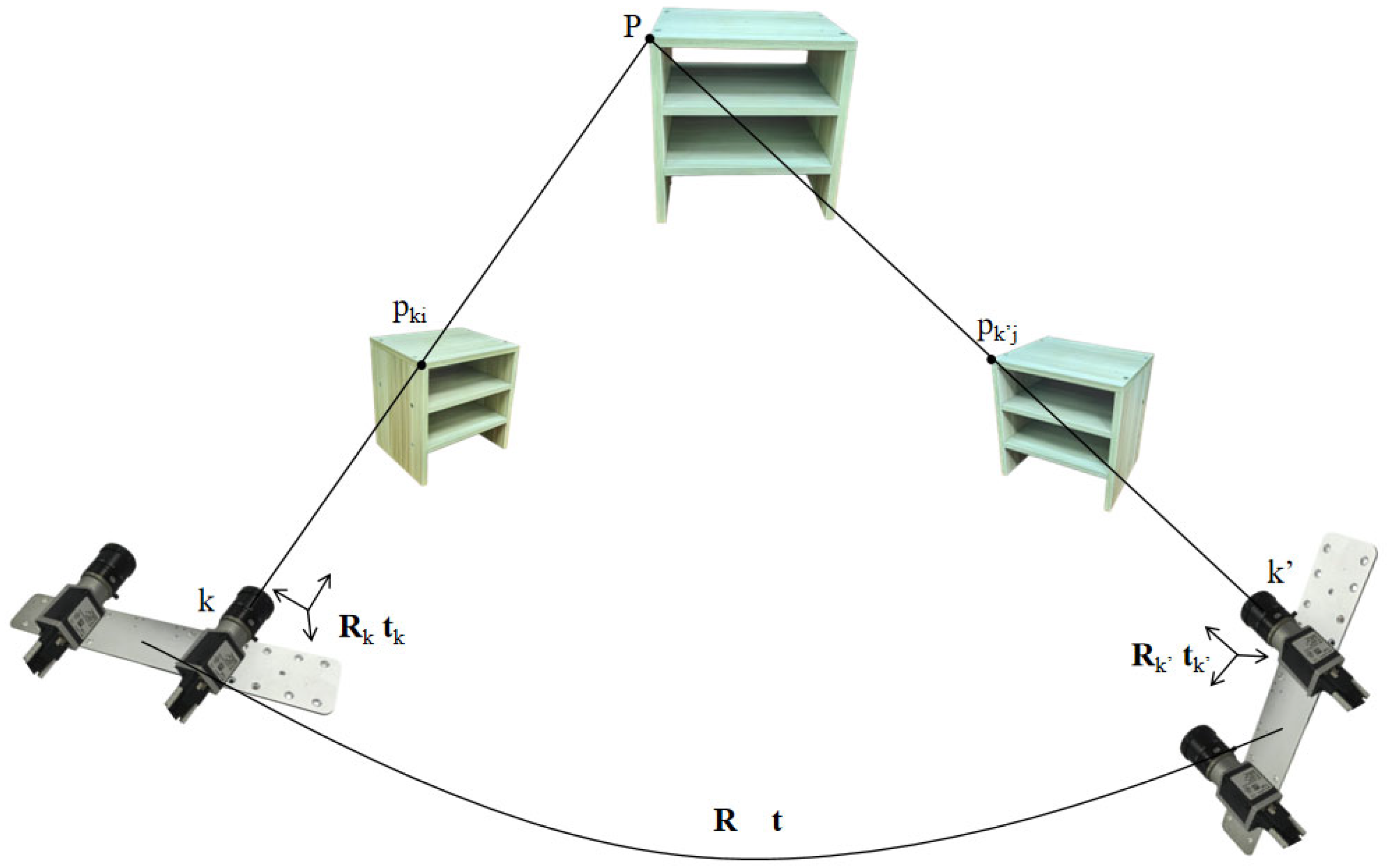
In a binocular camera system, the relative pose of the camera system satisfies the generalized epipolar constraint. Figure 1 shows this model, in which the imaging of a target point P by different cameras is represented as:

$$\left(p_{\mathrm{ki}},p_{ \mathrm{k} \prime \mathrm{j}},R_{\mathrm{k}},R_{ \mathrm{k} \prime },t_{\mathrm{k}},t_{ \mathrm{k} \prime }\right),$$

(1)

where $p_{ki}$ represents the pixel coordinates of point P on the image taken by camera k at moment i, and $p_{ \mathrm{k} \prime \mathrm{j}}$ represents the pixel coordinates of point P on the image taken by camera k′ at moment j. Moreover, $R_k$ and $R_{k^{\prime }}$ are the rotation matrices of camera k and camera k′, respectively, with respect to the multi-camera system, and $t_k$ and $t_{k^{\prime }}$ are the translation vectors of camera k and camera k′, respectively, with respect to the multi-camera system. If the matched pixel points at moments i and j come from the same camera, then $R_k=R_{k^{\prime }}$ and $t_k=t_{k^{\prime }}$.

Therefore, we can express the generalized polar line constraint by the following equation:

$$l_{k^{\prime }j}^T\left[\begin{array}{cc}E& R\\ R& 0\end{array}\right]l_{ki}=0.$$

(2)

In Equation (2), E represents the essential matrix, which can be expressed as:

$$E={\left[t\right]}_{\times }R.$$

(3)

Here, $R$ is the relative rotation matrix of the multi-camera system at adjacent moments, $t$ is the relative displacement vector, and ${[ ]}_{\times }$ represents the antisymmetric matrix of vectors. Finally, $l_{ki}$ and $l_{k^{\prime }j}$ represent the corresponding set of Plücker lines at moments i and j and are expressed as follows:

$$l_{ki}=\left(\begin{array}{c}{f}_{ki}\\ t_k\times f_{ki}\end{array}\right), l_{k^{\prime }j}=\left(\begin{array}{c}{f}_{k^{\prime }j}\\ t_{k^{\prime }}\times f_{k^{\prime }j}\end{array}\right),$$

(4)

where $f_{ki}$ and $f_{k^{\prime }j}$ are expressed as follows:

$$f_{ki}={\displaystyle \frac{\left(R_k{x}_{ki}\right)}{‖R_k{x}_{ki}‖}},f_{k^{\prime }j}={\displaystyle \frac{\left(R_{k^{\prime }}{x}_{k^{\prime }j}\right)}{‖R_{k^{\prime }}{x}_{k^{\prime }j}‖}},$$

(5)

where $x_{ki}=K^{-1}{p}_{ki}$ and $x_{k^{\prime }j}=K^{-1}{p}_{k^{\prime }j}$. In practical applications, cameras typically have square pixels, and the principal point is located at the center of the image. Therefore, the focal lengths of the two axes of the camera are equal. We hence obtain

$$\mathbf{K}=\mathrm{diag}\left(f,f,1\right).$$

(6)

Then, ${\mathbf{K}}^{-1}$ can be expressed as

$${\mathbf{K}}^{-1}=\mathrm{diag}\left(g,g,1\right),$$

(7)

where f is the camera focal length and $g=f^{-1}$. Generally speaking, in a multi-camera system, the baseline between cameras is relatively small, and the cameras obtain the best image quality at a similar focal length. Therefore, it is reasonable to assume that these cameras use the same focal length.

Because we rigidly connect the IMU to the camera and the relationship between the camera and the IMU has been calibrated, the IMU can provide the pitch and roll angles at moments i and j, and the Y-axis of the multi-camera coordinate system can be aligned to the direction of gravity. At this point, let θ be the rotation angle of the multi-camera system around the Y-axis. Using Carley’s formula, we obtain the rotation matrix as follows:

$$R_y={\displaystyle \frac{1}{1+s^2}}\left[\begin{array}{ccc}1-s^2& 0& 2s\\ 0& 1& 0\\ -2s& 0& 1-s^2\end{array}\right],$$

(8)

where $s=\tan (\theta /2)$ and $R_y$ is the rotation matrix after the Y-axis of the multi-camera coordinate system has been aligned with the direction of gravity. Then, we use $\tilde{t}$ to represent the translation vector of the multi-camera system and obtain

$$R={(R_{imu}^j)}^T{R}_y{R}_{imu}^i,$$

(9)

$$t={\left(R_x^j{R}_z^j\right)}^T\tilde{t}={\left(R_{imu}^j\right)}^T\tilde{t}.$$

(10)

Next, Equation (2) can be transformed into:

$${\left(\left[\begin{array}{cc}{R}_{imu}^j& 0\\ 0& R_{imu}^j\end{array}\right]l_{k^{\prime }j}\right)}^T\cdot \left[\begin{array}{cc}{\left[\tilde{t}\right]}_{\times }{R}_y& R_y\\ R_y& 0\end{array}\right]\cdot \left(\left[\begin{array}{cc}{R}_{imu}^i& 0\\ 0& R_{imu}^i\end{array}\right]l_{ki}\right)=0.$$

(11)

Substituting Equation (4) yields

$${\left(\left[\begin{array}{c}{R}_{imu}^j{f}_{k^{\prime }j}\\ R_{imu}^j\left(t_{k^{\prime }}\times f_{k^{\prime }j}\right)\end{array}\right]\right)}^T\cdot \left[\begin{array}{cc}{\left[\tilde{t}\right]}_{\times }{R}_y& R_y\\ R_y& 0\end{array}\right]\cdot \left(\left[\begin{array}{c}{R}_{imu}^i{f}_{ki}\\ R_{imu}^i\left(t_k\times f_{ki}\right)\end{array}\right]\right)=0.$$

(12)

Since the IMU can provide rotation angles in two directions relatively precisely, the degrees of freedom for the rotation matrix of the multi-camera system are reduced to one. Here, the degrees of freedom of the translation vector and the camera focal length are three and one, respectively. Therefore, we need at least five feature point pairs to complete the solution. Reorganizing this equation and extracting the coefficient matrix of $\tilde{t}$, we obtain

$${\left(\begin{array}{c}\left(R_{imu}^i{f}_{k^{\prime }j}\right)\times R_y\left(R_{imu}^i{f}_{ki}\right)\\ O_1\end{array}\right)}^T\hat{t}={\displaystyle \frac{M}{1+s^2}}\widehat{t}=0,$$

(13)

where $\hat{t}={[\begin{array}{cc}\tilde{t}& 1\end{array}]}^T$. Matrix M is a 5 × 4 matrix that only contains the unknowns f and s. Since Equation (13) has a non-zero solution, any 4 × 4 determinant formed by taking any four rows from matrix M is zero. This gives us ${\mathrm{C}}_5^4=5$ equations, which are:

$$\left\{\begin{array}{c}\det ({\mathbf{M}}_{1234}\prime )=0\\ \det ({\mathbf{M}}_{1235}\prime )=0\\ \det ({\mathbf{M}}_{1245}\prime )=0\\ \det ({\mathbf{M}}_{1345}\prime )=0\\ \det ({\mathbf{M}}_{2345}\prime )=0\end{array}\right.,$$

(14)

where ${\mathbf{M}}_l\prime$ is a new matrix formed by taking the elements of the l-th row of matrix M. Extracting the coefficients of the focal length f from the system of equations, we obtain

$$C(s)X=0.$$

(15)

Here,

$$X={\left(\begin{array}{lllllll}1\hfill & g\hfill & g^2\hfill & g^3\hfill & g^4\hfill & g^5\hfill & g^6\hfill \end{array}\right)}^T.$$

(16)

Matrix $X$ contains seven monomials, and the number of equations in Equation (15) is five. To make the number of equations and monomials equal, the first three equations in Equation (15) are each multiplied by g. Equation (15) can then be rewritten as:

$$C^{\prime }(s)X^{\prime }=0,$$

(17)

where

$$X^{\prime }={\left(\begin{array}{llllllll}1\hfill & g\hfill & g^2\hfill & g^3\hfill & g^4\hfill & g^5\hfill & g^6\hfill & g^7\hfill \end{array}\right)}^T.$$

(18)

Since the highest degree of s is eight, Equation (17) can be expanded as follows:

$$(s^8{C}_8^{\prime } +s^7{C}_7^{\prime }+s^6{C}_6^{\prime }+s^5{C}_5^{\prime }+s^4{C}_4^{\prime }+s^3{C}_3^{\prime }+s^2{C}_2^{\prime }+s{C}_1^{\prime }+C_0^{\prime })X^{\prime }=0.$$

(19)

The unknown s can be obtained from the eigenvalues of matrix G, which is represented as:

$$G=\left[\begin{array}{cccc}0& I& \cdot \cdot \cdot & 0\\ 0& 0& \cdot \cdot \cdot & 0\\ \cdot \cdot \cdot & \cdot \cdot \cdot & \cdot \cdot \cdot & I\\ -C_8^{\prime -1}{C}_7^{\prime }& -C_8^{\prime -1}{C}_6^{\prime }& \cdot \cdot \cdot & -C_8^{\prime -1}{C}_0^{\prime }\end{array}\right].$$

(20)

Using the Schur method, we solve for the eigenvalues and corresponding eigenvectors L of matrix G. Here, g can be obtained from the eigenvector, and the focal length $f=g^{-1}$. Once f and s have been calculated, they are substituted into matrix M. Any four rows from matrix M are selected to form a submatrix, and its eigenvector is computed as $\hat{t}={[\begin{array}{cc}\tilde{t}& 1\end{array}]}^T$. Finally, the relative poses of the system are computed using Equations (9) and (10).

Table 1. Minimal solution for relative pose estimation of a binocular camera with unknown focal lengths.

Method	Minimal Solution for Relative Pose Estimation
Application conditions:	Binocular camera with unknown focal length
Known conditions:	The pixel coordinates of three pairs of feature points in the images of the camera 1 at two adjacent moments ${\left(p_{1\mathrm{i}},p_{1\mathrm{j}}\right)}_3$, the pixel coordinates of two pairs of feature points in the images of camera 2 at two adjacent moments ${\left(p_{2\mathrm{i}},p_{2\mathrm{j}}\right)}_2$, the roll and pitch angles of the binocular camera system provided by IMU, rotation matrices and transtranslation vector of camera 1 and camera 2 with respect to the multi-camera system $\left(R_1,R_2,t_1,t_2\right)$.
Parameters to be estimated:	The rotation matrix R, translation vector t and camera focal length f between adjacent two frames.
1:	Using the given conditions, construct the Planck line I through Equations (4)–(7), I contains a parameter to be estimated, the camera focal length f.
2:	Equation (2) is constructed through the Planck line I based on the generalized polar line constraints, and R is the relative rotation matrix of the parameter to be estimated, and t is the relative translation vector of the parameter to be estimated.
3:	Using the original observations of the IMU, we can easily obtain the precise pitch and roll angles between adjacent moments. Since the IMU is fixedly connected to the camera system, the Y-axis of the multi-camera coordinate system can be aligned to the vertical direction. Therefore, parameters R and t that need to be estimated can be rewritten to Equations (9) and (10).
4:	Substitute Equations (9) and (10) into Equation (2), and extract the coefficient matrix of t. The equation is transformed into Equation (13).
5:	Since Equation (13) has a non-zero solution, based on the properties of the determinant, we can obtain the system of Equation (14).
6:	Extracting the coefficient matrix of the camera focal length f from Equation (14) and organizing it, Equation (19) can be obtained.
7:	Generate the matrix G and use the Schur method to solve the eigenvalues and corresponding eigenvectors of the matrix, thereby obtaining the camera focal length f and rotation angle parameters s.
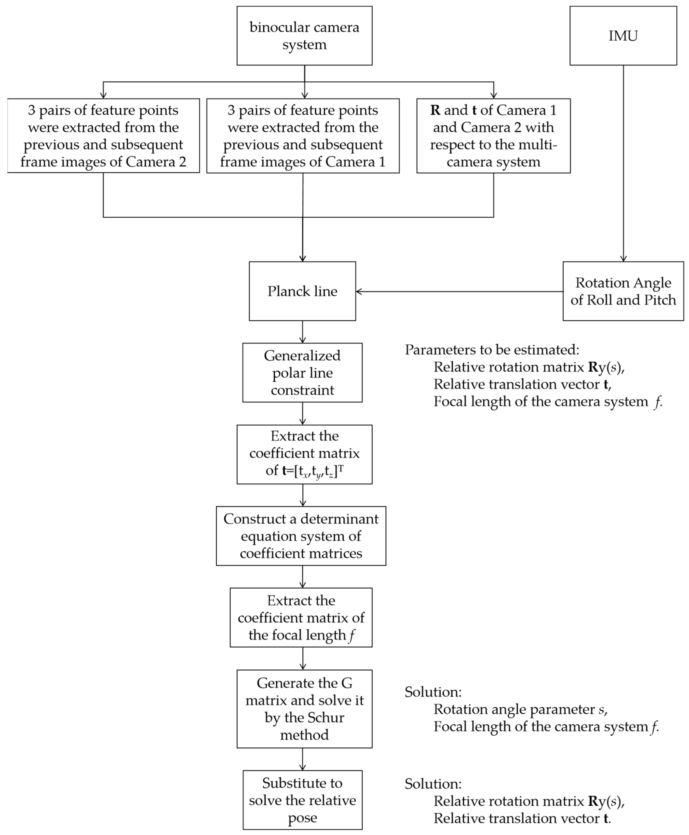
8:	Substitute the calculation results into Equations (8–10) to obtain the relative rotation matrix R and the relative displacement vector t.

presents the pipeline of our proposed minimal solution for relative pose estimation of a binocular camera system with unknown focal lengths. Meanwhile, we have also provided the flowchart of the algorithm, as shown in Figure 2.

4. Results

We evaluated the performance of our method and compared it with current classical methods. We selected two classic algorithms for comparison: the 17-point method proposed by Li [14] and the 6-point method proposed by Kneip [19], which we refer to as the 17-pt and 6-pt methods. We conducted experiments using both simulated and real data for a binocular camera system to compare the three algorithms.

To accurately compare the performance of different methods, we employed the following error assessment formulas for the camera focal length, rotation matrix, and translation vector. The error in the camera focal length f can be expressed as:

$${\xi }_{f_i}={\displaystyle \frac{\left|f_{ic}-f_{ig}\right|}{f_{ig}}},$$

(21)

where $f_g$ and $f_c$ denote the ground-truth and calculated focal lengths, respectively.

The error of the relative rotation matrix can be expressed as:

$${\xi }_R=\arccos \left({\displaystyle \frac{trace\left({\mathbf{R}}_g{{\mathbf{R}}_c}^T\right)-1}{2}}\right),$$

(22)

where ${\mathbf{R}}_g$ and ${\mathbf{R}}_c$ denote the ground-truth and calculated rotation matrices, respectively.

The relative translation vector error ${\xi }_t$ is defined as follows:

$${\xi }_t=\arccos {\displaystyle \frac{{\mathbf{t}}_g^T{\mathbf{t}}_c}{‖{\mathbf{t}}_g‖‖{\mathbf{t}}_c‖}},$$

(23)

where ${\mathbf{t}}_g$ and ${\mathbf{t}}_c$ denote the ground-truth and calculated translation vector, respectively.

4.1. Synthetic Data

We constructed a randomly generated simulated scene and created a series of 3D points with XYZ axes randomly distributed within the range of [−10, 10] m. The camera focal length was set to range from 100 to 1000, the camera resolution was set to 1000 × 700, and the principal point P0 was set to (500, 350). The extrinsic parameters between the two cameras were known and set to be less than 30 cm. The generated 3D points were projected into the pixel coordinate system to obtain their pixel coordinates. 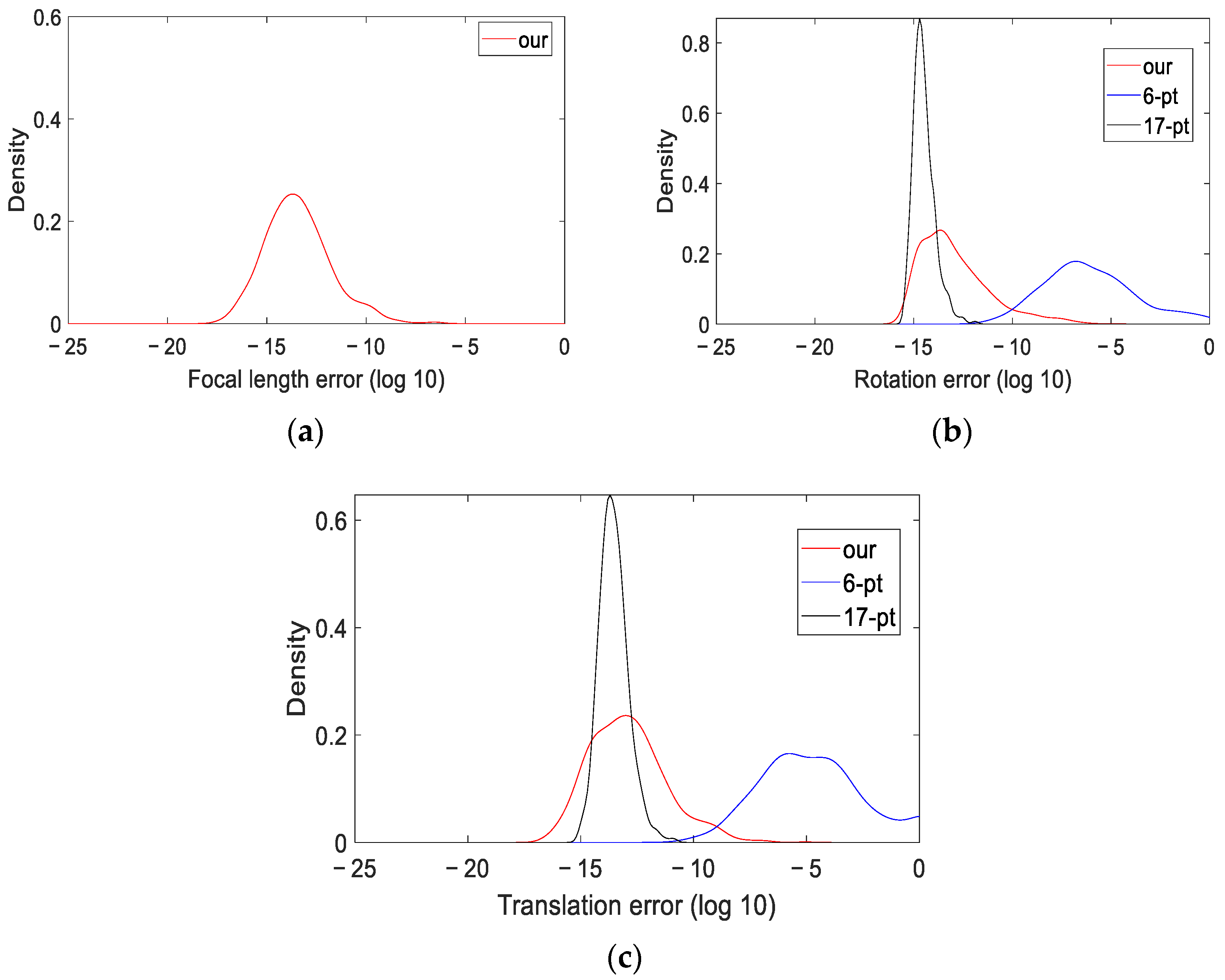We set the virtual camera to move continuously 10,000 times, with the rotation matrices around the x-axis and z-axis set to known values, simulating the rotation angles obtained through the IMU. We statistically analyzed the calculation errors of the focal length, relative rotation matrix, and relative translation vector under noise-free conditions. We present the probability density distribution of the errors in the figure, where Figure 3a depicts the focal length error, Figure 3b depicts the rotation matrix error, and Figure 3c represents the translation vector error.

In the graphs in Figure 3, the horizontal axis represents the logarithmic results of the calculation errors, and the vertical axis is the probability density. When the curve is on the left side of the graph, it indicates that the method has a smaller calculation error and higher numerical stability. Since the current classic methods usually require that the intrinsic parameters of the camera be fully known when performing pose estimation and cannot calculate the focal length of the camera, only the error probability distribution curve of the focal length estimated by our method is shown in Figure 3a. The distribution of the curve and the horizontal axis coordinates reveal that our method accurately determines the focal length of the camera. The error probability density curves of the rotation matrix and translation vector are quite similar. All three methods can produce relatively accurate results, but the proposed and 17-point methods are more precise. However, in contrast to the 17-point method, which requires 17 point correspondences, the proposed algorithm only needs 5 point correspondences to complete the calculation. When combined with the RANSAC algorithm, its computational efficiency is improved. To more accurately analyze the performance of the three algorithms, we have listed the median errors of the calculation result in

Table 2. The median of errors calculated using different methods based on simulated data.

	Our	17-pt [14]	6-pt [20]
${\xi }_f$-Median	2.7425 × 10−14
${\xi }_R$-Median/Deg	1.5366 × 10−14	2.6390 × 10−15	4.4990 × 10−7
${\xi }_t$-Median/Deg	8.5123 × 10−14	2.5599 × 10−14	1.5580 × 10−5

. Here, ξ_f denotes the camera focal-length error, ξ_R denotes the rotation-matrix error, and ξ_t denotes the translation-vector error. From the data in the table, we can infer that the proposed algorithm is close to the 17-point method in stability and better than the 6-point method. Moreover, it can calculate the camera focal lengths.

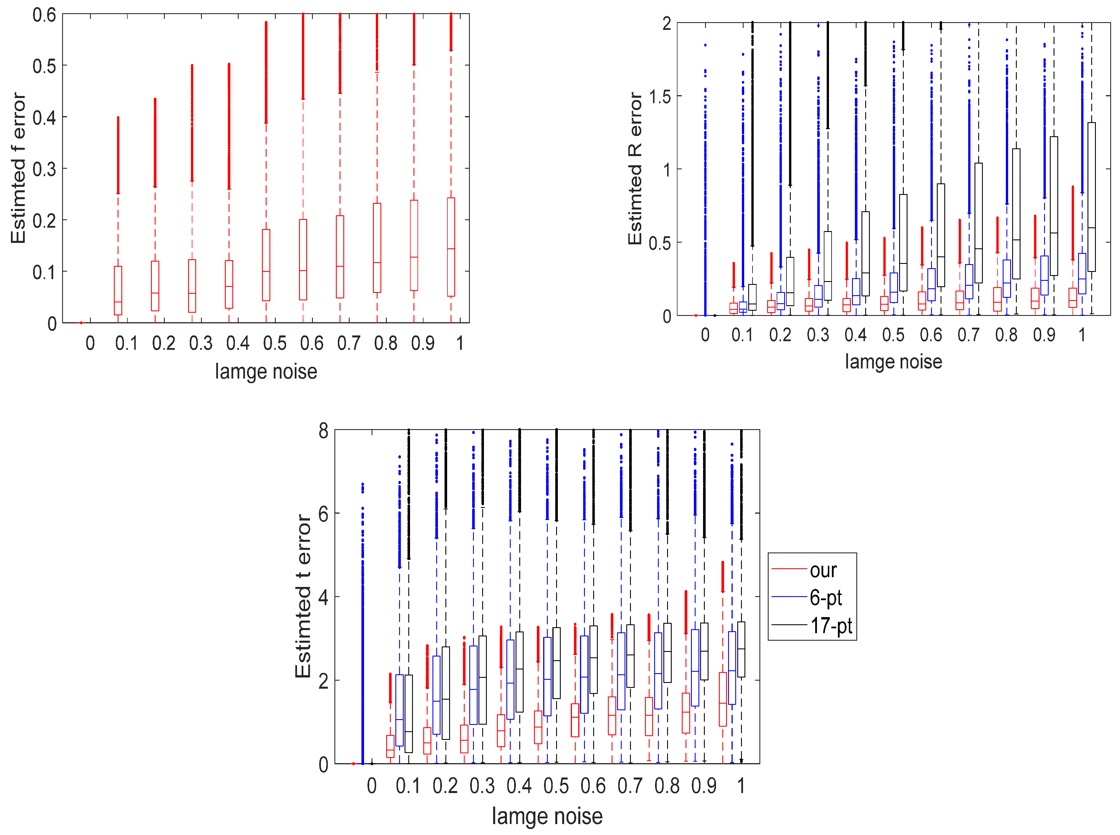
In engineering applications, the pixel coordinates of feature point pairs must be obtained using feature point extraction and matching algorithms, which inevitably introduce pixel errors. To further analyze the influence of different levels of noise on the algorithm, we introduced random noise to the pixel coordinates in the previous noise-free dataset. After analyzing the performance of feature extraction and matching algorithms and referencing the existing literature, we set the noise coefficient to range from 0 to 1, and the intervals of the coefficient were set to 0.1 [10,28,29,30]. 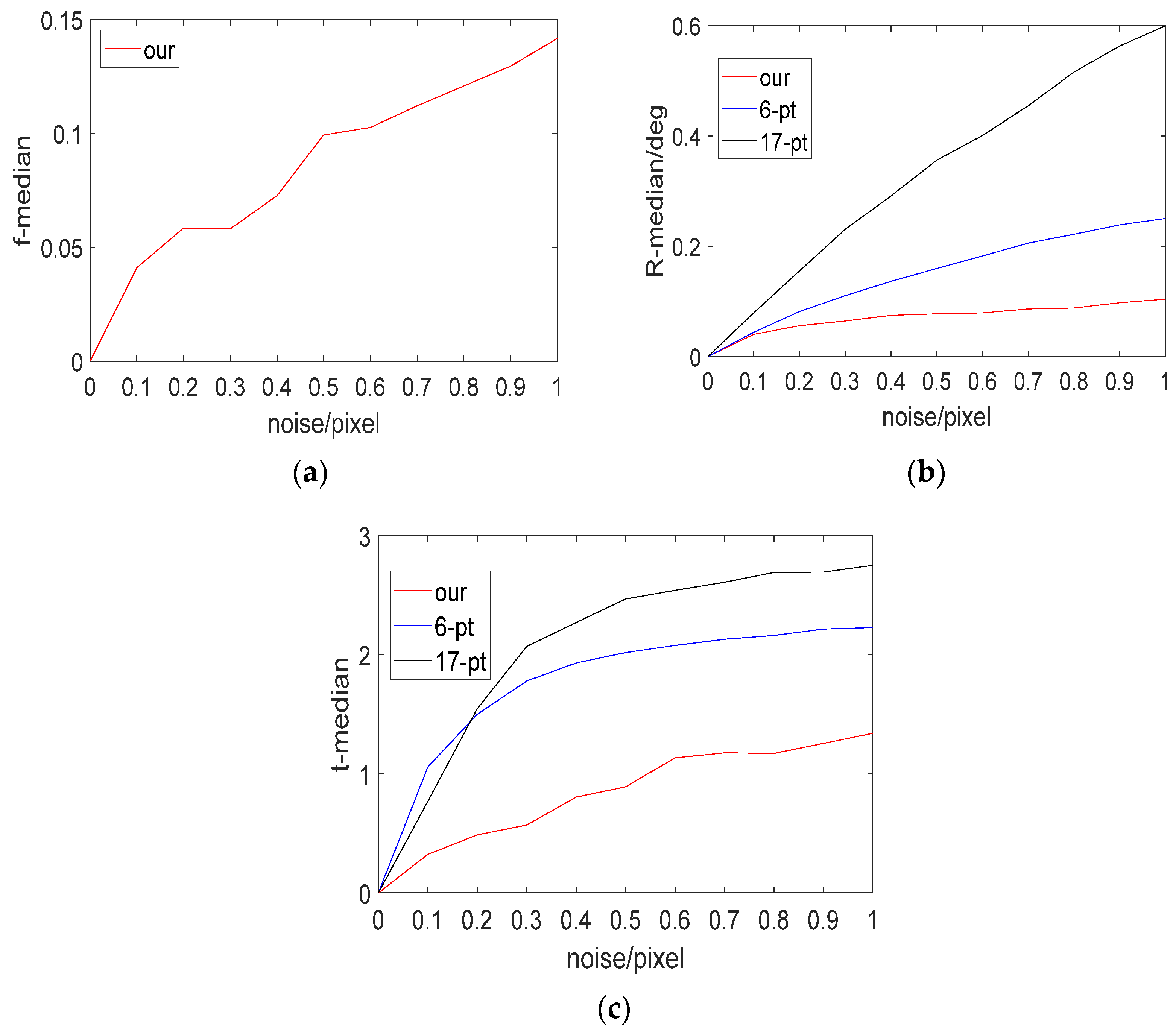We calculated the results of running the three models 10,000 times under different coefficient errors and statistically analyzed the errors of the focal length f, rotation matrix R, and translation vector t. We plot the median variation in the calculation errors under different levels of image noise in Figure 4.

According to Figure 4a, the error in focal length calculation increases with the increase in pixel coordinate error. However, when the noise coefficient is 1, the error in the focal length is less than 0.15, which meets typical requirements. Figure 4b,c clearly show that the calculation error in the 17-point method increases the most with increases in pixel coordinate error, followed by the error of 6-point method, while the error of our method is the smallest and its performance is the best. To more accurately visualize the calculation errors of the three methods, we also provide box plots of the calculation errors of the three methods for noise coefficients ranging from 0 to 1, as shown in Figure 5.

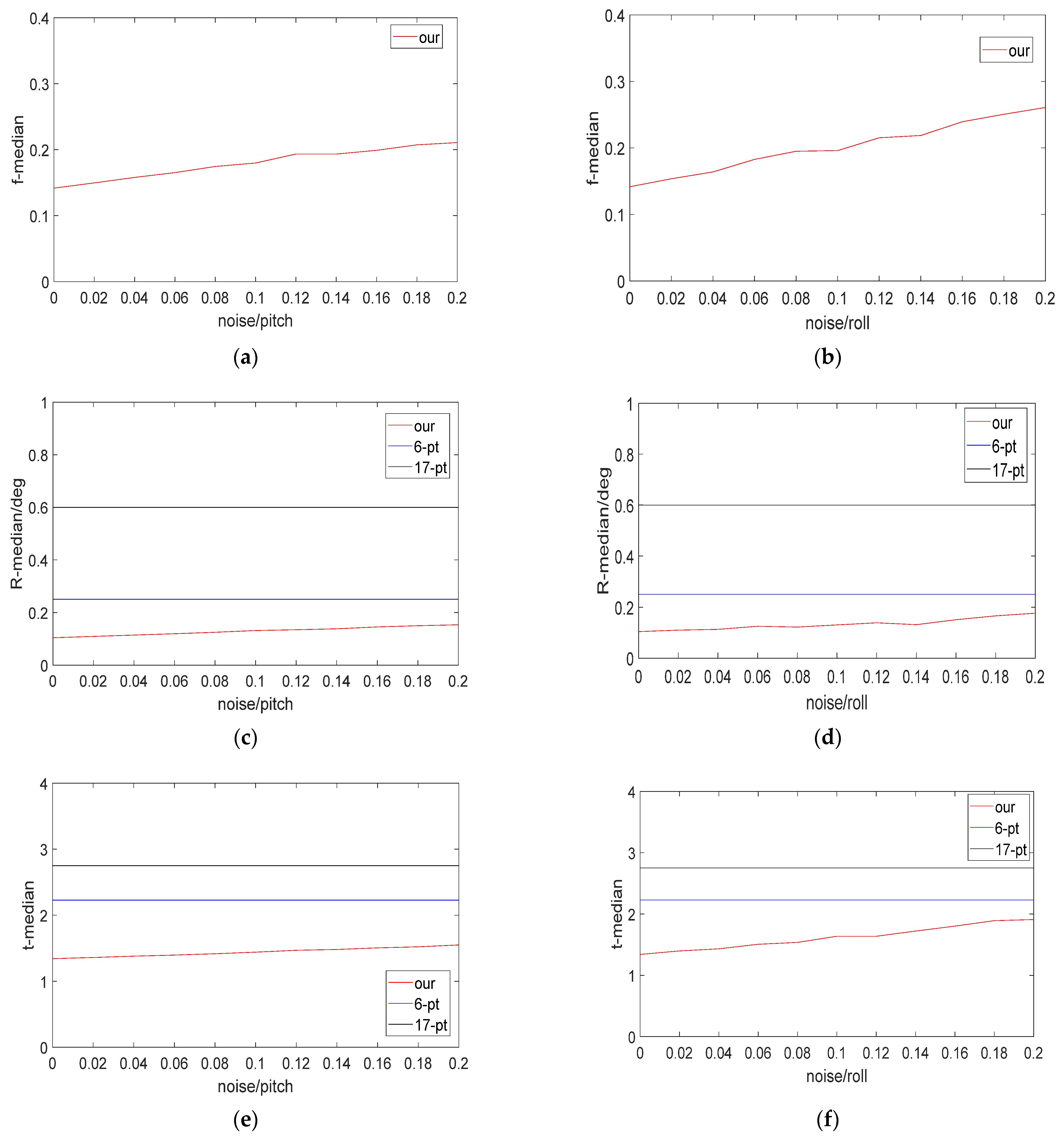
All IMUs have measurement and solution errors. Since our proposed algorithm uses an IMU to obtain part of the rotation matrix, we further added IMU errors to the data with a pixel error noise coefficient of 1 to more accurately simulate the algorithm’s performance in real situations. Considering that the time interval between adjacent frames of the camera is relatively short and the angle accuracy provided by the IMU is relatively high, we added random noise ranging from 0° to 0.2° respectively to the pitch and roll angles provided by IMU [31]. The median error curves of the calculations are shown in Figure 6. The first row is the camera focal length error curve after introducing IMU errors, the second row shows the rotation matrix error curve, and the last row shows the translation vector error curve. The first and second columns in Figure 6 show the calculation results with pitch angle and roll angle errors introduced, respectively.

Since the 6-point method and the 17-point method do not use the IMU to obtain partial rotation angles, the curves for 6-pt and 17-pt in the figure are constant values equal to the median errors of the calculation results when pixel coordinate error with a coefficient of 1 is introduced. It can be seen from the figure that even with the addition of 0.2° of IMU noise, the calculation error of our method remains the smallest.

4.2. Real Data

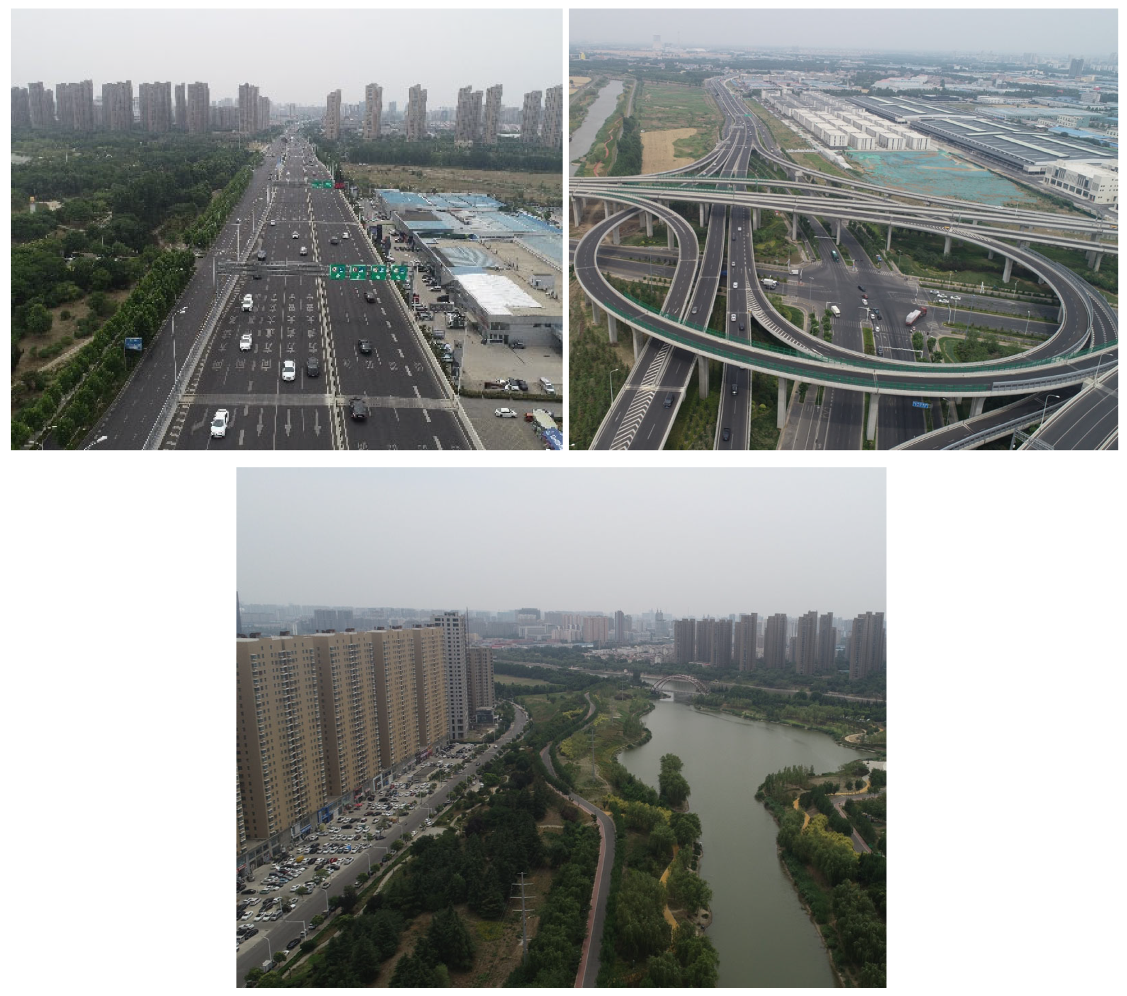
To evaluate the reliability of our method more fully, we collected a series of image data in an outdoor real-world scenario using a drone. We mounted two Basler acA1300-60gc color cameras and an IMU module on a drone, rigidly connecting them together and pre-calibrating their positional relationships. The IMU module was used to obtain partial rotation angles of the system. Prior to data collection, we ensured that the drone remained stationary for a period to complete the initial alignment of the IMU, thereby obtaining more accurate IMU output results. We amassed a comprehensive dataset comprising 20,000 images from diverse scenarios to rigorously evaluate the algorithm’s performance. Example images from the dataset are shown in Figure 7.

In addition to the above, the drone was also equipped with a GNSS module, which was used to obtain its 3D coordinates and provide the ground truth for the relative pose of the drone. At the same time, the PPS pulse signal received by the GNSS module was used to synchronize the times of the cameras and IMU, realizing simultaneous image capture by multiple cameras. After all images were acquired, the SIFT algorithm was employed to extract the corresponding matching points from the images captured by the camera system at different moments [32]. 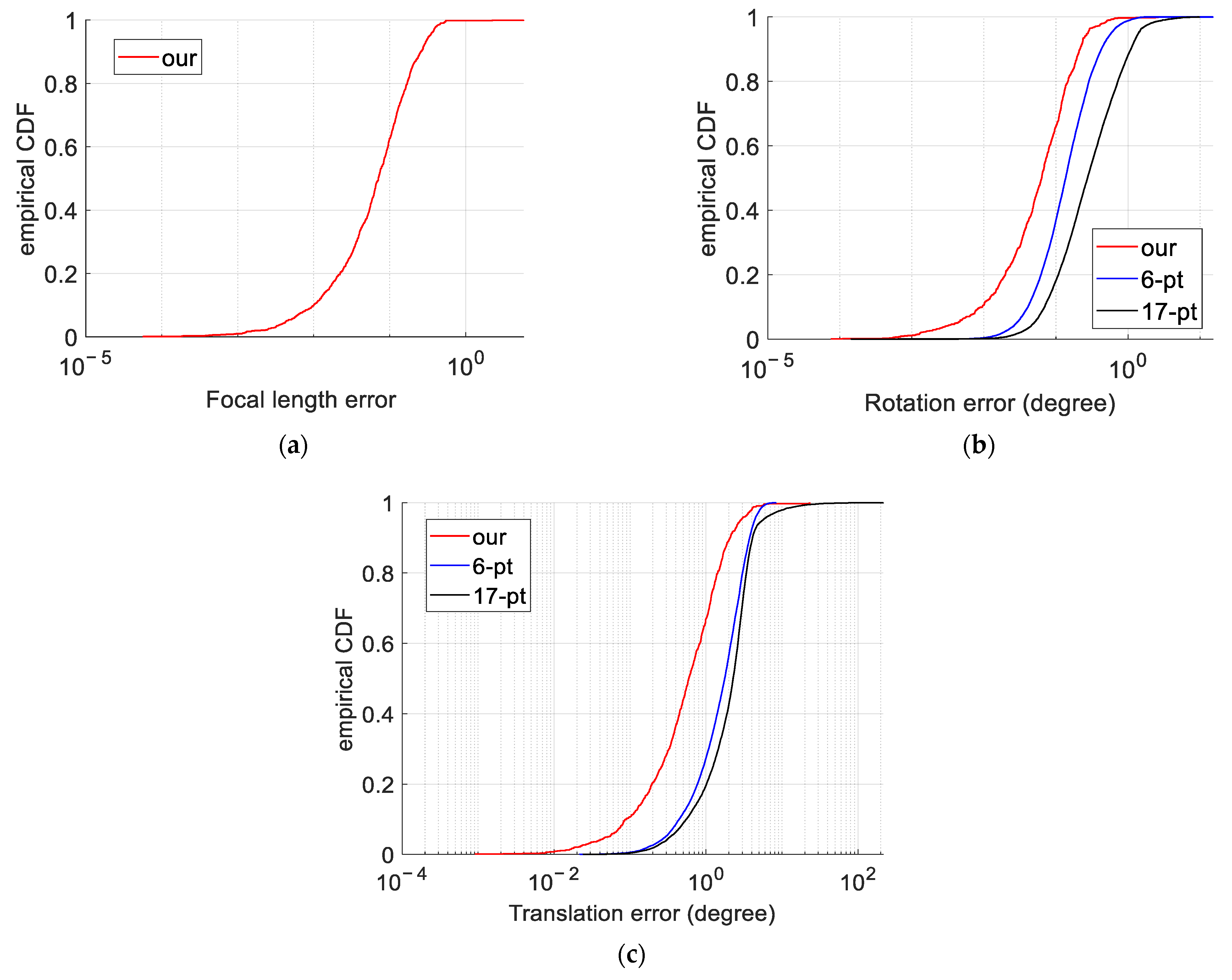Finally, we used the matched corresponding feature points to solve the relative pose and camera focal length with the three algorithms combined with the RANSAC algorithm [33]. We evaluated the three algorithms on the real data and plotted the cumulative distribution functions (CDFs) of the calculation results in Figure 8. In this figure, the closer the curve is to the left, the smaller the calculation error. By comparing the positions and trends of the three curves in the figure, the following findings can be obtained: the accuracy of the relative pose calculated by the 17-point method is the poorest; the 6-point method has a steeper slope to its curve, indicating better computational stability; and the calculation error of our method is the smallest.

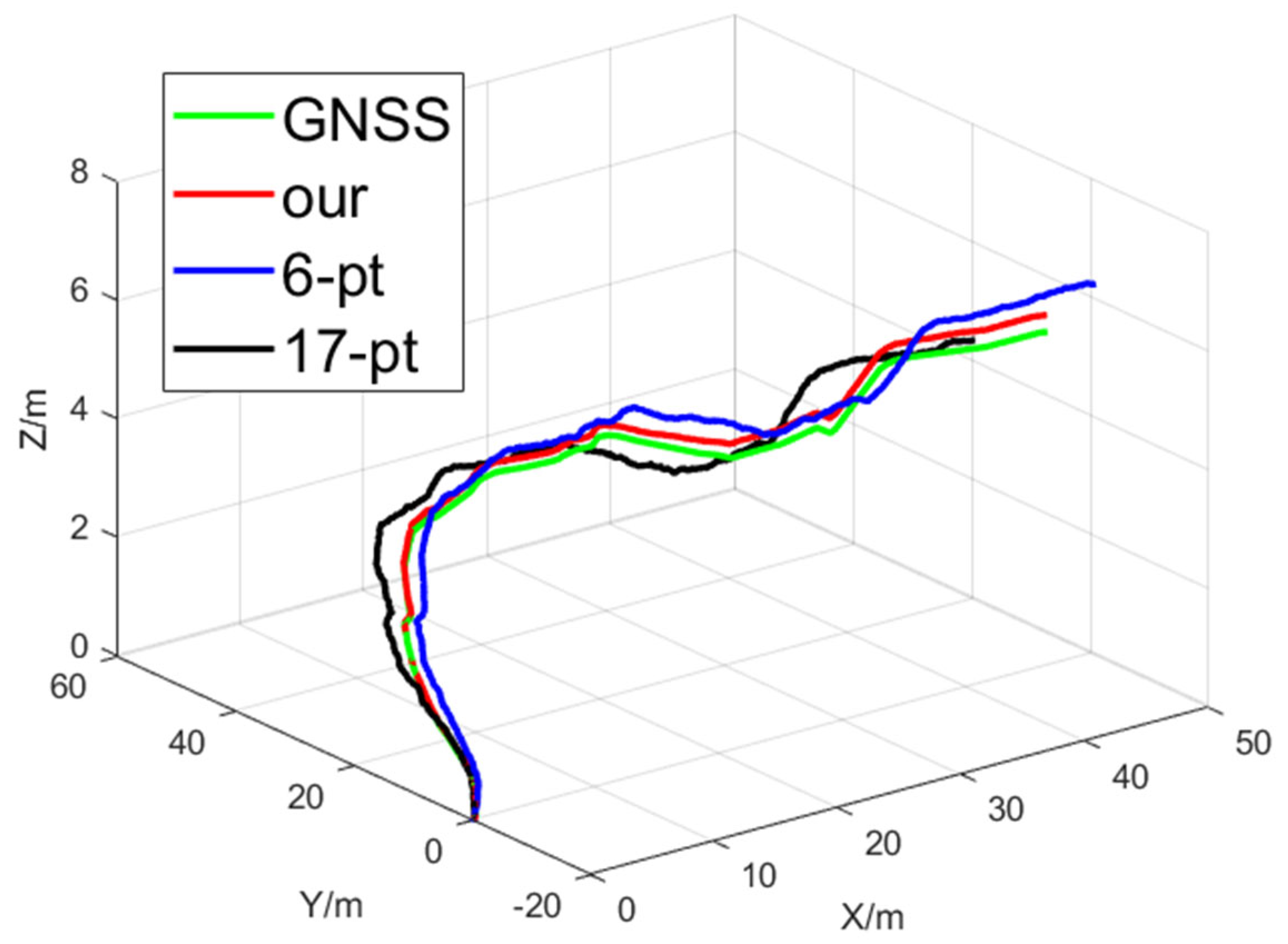
To analyze how algorithmic accuracy evolves over time, we selected one data segment and plotted the GNSS-based ground-truth trajectory alongside the trajectories derived from the relative poses computed by the three methods; the results are shown in Figure 9. All trajectories were initialized at (0, 0, 0) to intuitively compare the different approaches. The green curve represents the reference trajectory. It can be observed that the proposed algorithm ensures that its computed results do not diverge over the entire observed time interval, preserving stable convergence and exhibiting the smallest deviation from the reference trajectory.

In

Table 3. Comparison of calculation errors based on real data.

		${\mathit{\xi }}_{\mathit{f}}$	${\mathit{\xi }}_{\mathit{R}}$/deg	${\mathit{\xi }}_{\mathit{t}}$/deg
Our	Mdeian	0.071	0.063	0.591
	SD	0.218	0.152	1.525
6-pt	Mdeian		0.136	1.758
	SD		0.286	1.292
17-pt	Mdeian		0.276	2.271
	SD		0.696	4.167

, we present the median and standard deviations of the errors calculated by the different algorithms to analyze the calculation errors on real data more clearly. Table 3 reveals that when evaluated on the real data collected by the drone, the 17-point method has the largest errors in the calculated relative rotation matrix R and relative translation vector t, and our proposed algorithm has the smallest median and standard deviation of calculation errors. Compared with the 6-pt method, the proposed algorithm reduces the median error in the rotation matrix by 54% and by 66% in the translation vector. Compared with the 17-point method, our proposed algorithm reduces the median error in the rotation matrix by 77% and by 74% in the translation vector. These results indicate that our method possesses better stability and accuracy.

5. Discussion

To evaluate the performance of our proposed algorithm, we first generated a synthetic dataset. Experiments on this idealized data verified the numerical stability of the method. As shown in Table 2, compared with the 6-point algorithm, our approach exhibits markedly higher numerical stability, and relative to the 17-point method, it requires far fewer minimum point correspondences while maintaining the same order of magnitude in accuracy. Next, to analyze the influence of the main noise sources, we successively introduced image errors and IMU errors into the synthetic dataset. The results show that our algorithm has a stronger anti-interference ability compared with the reference method. Finally, we collected a series of real-world datasets using a UAV and evaluated the algorithm’s performance under practical conditions. The trends observed on real data closely match those on synthetic data: when the input data contain errors, the 17-point method yields the lowest accuracy, followed by the 6-point method, while our algorithm achieves the highest accuracy. This confirms the reliability and practicality of our approach. In addition, we present the estimated trajectories of the real datasets and analyze the temporal evolution of the estimation error, which further shows that the results produced by our algorithm converge well over time.

Although the proposed algorithm significantly outperforms the classical 17-point and 6-point methods in terms of accuracy, there is still room for further improvement. Our current work focuses on optimizing the geometric-constraint-based algorithm for relative camera pose estimation. However, as shown in our experimental results, errors in feature-point extraction and matching severely degrade the accuracy of pose estimation. Therefore, enhancing the precision of feature extraction is a promising direction for boosting both the accuracy and robustness of relative pose estimation. Moreover, in real-world applications, apart from point features, there are abundant line and planar features. Integrating these additional cues into the pose estimation method represents another viable avenue for improvement.

6. Conclusions

For scenarios that include multi-camera systems with unknown focal lengths, we proposed a minimal solution for estimating the relative pose. Leveraging the high accuracy of IMUs over short time intervals, we rigidly connected an IMU to the camera system and used the IMU to obtain the roll and pitch rotation angles of the system, which allows for a straightforward calculation of the system’s partial relative rotation matrix. This approach decreases the minimum number of corresponding point pairs required for calculating the relative pose of the multi-camera system, thereby decreasing the number of iterations in RANSAC and enhancing the reliability and accuracy of the algorithm. We generated simulated data to conduct a detailed analysis of the impact of different noise levels on the performance of the proposed algorithm and evaluated the reliability of the algorithm using real data collected by a drone. The results provide evidence that, comparing it with the current classic methods, our method reduces the errors in calculating the relative rotation matrix and translation vector of the multi-camera system by 54% and 66%, respectively. In addition, our method is also capable of estimating the camera focal length, thereby broadening the applicability of the algorithm.