Abstract
Accurate modeling of ionospheric variability is critical for space weather forecasting and GNSS applications. While machine learning approaches have shown promise, progress is hindered by the absence of standardized benchmarking practices and narrow test periods. In this paper, we take the first step toward fostering rigorous and reproducible evaluation of AI models for ionospheric forecasting by introducing IonoBench: a benchmarking framework that employs a stratified data split, balancing solar intensity across subsets while preserving 16 high-impact geomagnetic storms (Dst ≤ nT) for targeted stress testing. Using this framework, we benchmark a field-specific model (DCNN) against state-of-the-art spatiotemporal architectures (SwinLSTM and SimVPv2) using the climatological IRI 2020 model as a baseline reference. DCNN, though effective under quiet conditions, exhibits significant degradation during elevated solar and storm activity. SimVPv2 consistently provides the best performance, with superior evaluation metrics and stable error distributions. Compared to the C1PG baseline (the CODE 1-day forecast product), SimVPv2 achieves a notable RMSE reduction up to across various subsets under diverse solar conditions. The reported results highlight the value of cross-domain architectural transfer and comprehensive evaluation frameworks in ionospheric modeling. With IonoBench, we aim to provide an open-source foundation for reproducible comparisons, supporting more meticulous model evaluation and helping to bridge the gap between ionospheric research and modern spatiotemporal deep learning.
1. Introduction
The ionosphere, Earth’s upper atmospheric layer ionized by solar radiation, is integral to radio signal propagation but can introduce significant positioning errors, posing challenges for Global Navigation Satellite System (GNSS) applications [1]. In safety-critical domains such as civil aviation, operations like aircraft landing are constrained to the certified L1 frequency (1.5 GHz), which demands high positional accuracy. Ionospheric gradients and scintillation, particularly during geomagnetic disturbances, can degrade signal accuracy and threaten positioning integrity [2]. Beyond these storm-time effects, even under quiet geomagnetic conditions, post-sunset plasma-bubble scintillation in equatorial regions has been reported to occasionally lead to loss of lock [3,4]. To mitigate these effects, ground-based (GBAS) and Satellite-Based (SBAS) augmentation systems are used to provide ionospheric corrections and enhance signal reliability. These systems rely heavily on accurate modeling of ionospheric delays, which are typically quantified using the total electron content (TEC), the integrated electron density along a signal path, measured in TEC Units ().
As GNSS-enabled services continue to expand across sectors, TEC forecasting has become an active research area, with numerous predictive models proposed [5]. Yet, modeling the ionosphere remains inherently difficult due to its complex and highly dynamic behavior in response to solar and geomagnetic activity [6,7,8]. Existing strategies range from well-established empirical models, such as the International Reference Ionosphere (IRI) [9,10] and physics-based simulations [11,12], to more recent machine learning (ML)-based approaches. ML techniques have been reported to show improved accuracy compared to traditional models, supported by the growing availability of data and advances in artificial intelligence (AI) [13,14,15,16].
Motivated by the COSPAR 2015–2025 roadmap’s call for extended forecasting and multi-step prediction capabilities in space weather [17], recent studies have increasingly adopted recurrent neural networks (RNNs), particularly Long Short-Term Memory (LSTM) architectures to capture longer temporal dependencies in ionospheric behavior. For example, Kaselimi et al. [13] implemented a sequence-to-sequence LSTM approach for vertical TEC (VTEC), outperforming traditional baselines. Kim et al. [14] tailored their LSTM network for storm conditions, reporting improved accuracy compared to SAMI2 and IRI-2016. More recently, Ren et al. [18] presented a hybrid CNN–BiLSTM design that integrates geomagnetic indices such as Kp, ap, and Dst, focusing on storm conditions.
While LSTMs effectively capture temporal dynamics, they lack inherent spatial awareness without additional modules. Thus, in parallel, researchers have explored Convolutional LSTM (ConvLSTM)-based approaches to jointly model spatial and temporal structures. A foundational contribution in this direction is the work of Boulch et al. [19], who developed one of the few fully open-source AI models for ionospheric prediction. Their best-performing configuration, DCNN, stacked three ConvLSTM layers and applied a heliocentric transformation to account for Earth’s rotation. More recent studies have proposed alternative ConvLSTM-based architectures, often without referencing or benchmarking against DCNN. Liu et al. [20] refined the loss function and explored storm-specific training; Gao and Yao [21] introduced multichannel inputs, including solar and geomagnetic indices; and Yang et al. [16] showed that a TEC-only ConvLSTM could outperform both IRI-Plas and C1PG. Most recently, Liu et al. [22] focused on parameter optimization and incorporated skip connections and attention mechanisms, achieving improved predictive accuracy and generalization.
Despite these advances, the lack of common baselines makes it difficult to assess progress or establish consistent evaluation standards within the field. As a result, ionospheric ML research risks developing in isolation, without the cumulative rigor seen in more mature spatiotemporal modeling domains such as video prediction or weather forecasting. Shared evaluation practices are critical for both scientific and operational goals, as also emphasized by [23,24,25].
Toward this goal, we take an initial step toward establishing the needed evaluation standards and common baselines by developing the first iteration of IonoBench as a benchmarking framework for comprehensive ionospheric ML forecasting. With this framework we evaluate a DCNN [19] alongside two representative state-of-the-art (SOTA) models adapted from recent spatiotemporal benchmarks [26]: SwinLSTM [27] and SimVPv2 [28]. The performance of these AI models is benchmarked against the climatological reference (IRI 2020 [9]) model. Subsequently, the top-performing model is compared against C1PG, the CODE Analysis Center’s 1-day forecast product, to establish an operational reference point.
Furthermore, a recurring limitation in prior work is the narrow temporal scope of evaluation datasets, which often fail to reflect the full spectrum of ionospheric variability. Many studies have been confined to solar cycle 24 (SC24), a period marked by relatively low solar activity, limiting the stress-testing capacity of proposed models. In contrast, solar cycle 23 (SC23) included several of the most intense geomagnetic storms in recent decades and shows F10.7 trends more closely aligned with the ongoing solar cycle 25 (SC25) [29], making it a more operationally representative basis for model development and evaluation.
To address this, our framework proposes a carefully designed stratified data split that balances solar activity levels across training, validation, and test sets while explicitly preserving major geomagnetic storm events in the test set. This design enables robust, real-world evaluation scenarios that reflect both quiet and disturbed conditions, which is critical to forecast readiness. All datasets, split definitions, models, and configurations are released as open source on GitHub via the IonoBench repository: https://github.com/Mert-chan/IonoBench.git (accessed on 10 July 2025).
2. Data Overview
2.1. Data Description
This framework uses Global Ionosphere Map (GIM) final products from the International GNSS Service (IGS) [30]. These maps combine outputs from eight analysis centers and provide global vertical TEC at a spatial resolution of latitude by longitude, with a temporal resolution of 2 h. Seventeen auxiliary variables were sourced from NASA’s OmniWeb database [31] to support model conditioning on solar–terrestrial dynamics. These include:
- Solar Activity Index: 10.7 cm solar radio flux ()
- Geomagnetic Indices: Disturbance storm time index (), planetary index (), auroral electrojet index (), and polar cap index ()
- Solar Wind Parameters: Solar wind speed, density, temperature, dynamic pressure, and flow direction (longitude and latitude angles)
- Interplanetary Magnetic Field (IMF): Total magnitude (B), vertical component (), and coupling electric field (E)
- Time Features: Year, day of year, and hour to account for diurnal, seasonal, and solar cycle variability
The selection of auxiliary variables was guided by preliminary feature selection studies, leveraging correlation analyses between various solar–terrestrial indices and TEC statistics [32]. To avoid redundancy among highly correlated indices within the same physical category (e.g., solar activity), individual training comparisons led to the selection of a single representative, , for solar flux. Following this, a sequential backward selection [33] process identified a core set of influential features. This core set was further refined (e.g., by adopting in GSM coordinates instead of GSE, based on its established relevance in magnetosphere–ionosphere coupling [34]) and expanded with a comprehensive suite of solar wind parameters. This approach aimed to provide a rich, yet curated, input space for the diverse deep learning models under evaluation. The overall contribution of these input categories was subsequently evaluated using a feature ablation study (see Appendix A).
The dataset spans 1 January 2000 to 11 September 2024, and contains 108,251 GIMs. This period covers the solar maximum and decline of solar cycle 23 (SC23), all of solar cycle 24 (SC24), and the ascending phase of solar cycle 25 (SC25). It includes 88 classified geomagnetic storms (Dst nT), of which 80 are intense (e.g., nT nT) and 8 are superintense (Dst nT), following the criteria reported by Gonzalez et al. [35,36,37].
2.2. Preprocessing
The preprocessing of GIMs and auxiliary indices was performed to ensure consistent input formats and enhance model performance. The preprocessing steps are summarized below:
- GIM Preprocessing: IGS GIMs were first read from IONEX files. During reading, structural issues such as merged digits or malformed rows were automatically corrected to maintain consistent dimensions. For consistency with convolutional architectures, the original (lat × lon) GIMs were reshaped to a square grid by duplicating the first latitude row (87.5N) and removing the last longitude column (180E). Then, a two-stage outlier correction followed, involving both global and local stages (Appendix B). All GIM values were then normalized to using min–max scaling. Finally, a heliocentric transformation was applied following Boulch et al. [19] to align the subsolar point across all samples, compensating for Earth’s rotation and enabling the model to learn diurnal variations more effectively.
- OMNI Index Preprocessing: While reading, OMNI indices, originally sampled at a 1 h resolution, were downsampled to the 2 h cadence of the GIMs, and data cleaning was applied during the process (see Appendix B for details). Each index was normalized independently to using min–max scaling and reshaped into grids, consistent with the spatial structure of the GIMs. These were then stacked as additional input channels, providing all models with a consistent multichannel structure.
2.3. Data Splitting
Evaluating ionospheric models fairly requires a data split that reflects the full diversity of solar and geomagnetic activity. Prior studies have often adopted either chronological or window-based data splitting strategies. Chronological splits preserve temporal continuity but may overlook key variability across solar cycles due to a limited testing period [16,19,38]. Windowing approaches, such as sliding windows, introduce greater sample diversity but risk data leakage if temporal gaps are not inserted [20]. Alternatively, some studies use fixed-length windows around geomagnetic storms to support targeted modeling [21,22], but this approach reduces flexibility in balancing solar activity levels across the dataset, motivating the need for a more extensive strategy.
We address these challenges by implementing a multi-stage stratified data-splitting strategy, aiming for an approximate 70:15:15 (train–validation–test) distribution across the subsets. The distribution of samples is achieved by giving the highest priority to the rarest samples as follows:
- Step 1
- Storm-aware allocation: Superintense (Dst nT) and intense storms ( nT) were prioritized and distributed proportionally across train/val/test splits (see Table 1).
- Step 2
- Solar activity balancing: Afterwards, samples were binned by F10.7 into four solar classes (very weak, weak, moderate, intense) [39] and allocated to match the 70:15:15 ratio, with guard gaps by using non-storm periods to ensure no overlap between training, validation, and test subsets.

Table 1.
Storm Event Distribution.
Table 1.
Storm Event Distribution.
| Storm Class | Training | Validation | Testing |
|---|---|---|---|
| Intense ( Dst nT) | 54 | 12 | 14 |
| Superintense (Dst nT) | 5 | 1 | 2 |
As shown in Figure 1b, the proportions for each solar class in the test set range between 20% and 30%. While exact matching across all subsets is challenging, care was taken to ensure the training and validation sets also reflect a reasonably balanced distribution across these classes. This approach aimed to reduce biases tied to specific space weather regimes and allowed for rigorous testing of model generalization across varying conditions.
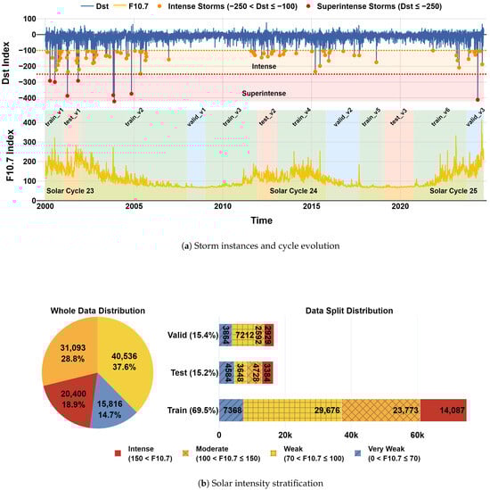
Figure 1.
Stratified data split: (a) Time series of F10.7 and , with subset periods containing storms highlighted; (b) Distribution of solar intensity classes in each split.
3. Experimental Setup
3.1. Models
This study benchmarks three deep learning architectures that span different archetypes for spatiotemporal forecasting.
DCNN [19] (DCNN121) is a recurrent architecture designed specifically for ionospheric TEC forecasting. It employs three stacked ConvLSTM layers with changing dilation factors (1-2-1) to expand the receptive field and better predict diverse geophysical behaviors.
SwinLSTM [27] combines a simplified LSTM recurrence with hierarchical Swin Transformer blocks. This hybrid architecture leverages local-window self-attention and patch-based processing to model global spatial dependencies while maintaining temporal continuity with the LSTM module.
SimVPv2 [28] represents a non-recurrent baseline based on pure convolutional processing. It separates spatiotemporal modeling into three components: a spatial encoder, a temporal translator (gated spatiotemporal attention (gSTA) is used in this work), and a decoder. Its fully convolutional nature makes it computationally efficient while maintaining high accuracy across diverse conditions.
For RNN-based models (DCNN and SwinLSTM), training was performed using teacher forcing [40] to mitigate error accumulation during multi-step forecasting. All models output multi-frame predictions in parallel, enabling direct comparison of long-horizon accuracy and stability.
3.2. Training
Each model was trained with a multichannel input tensor of shape , where B is the batch size; C the number of input channels (including auxiliary features); is the temporal input length, predicting the subsequent steps (24 h); and representing the spatial resolution.
Training was carried out using Distributed Data Parallel (DDP) on four NVIDIA RTX 5000 GPUs (24 GB each). The learning rate range test was used to select the initial learning rate, followed by a ReduceLROnPlateau scheduler and early stopping (maximum 50 epochs). All models were trained using the same pipeline for consistency.
3.3. Testing
3.3.1. Evalution Framework
The framework testing design follows the flowchart below (Figure 2).
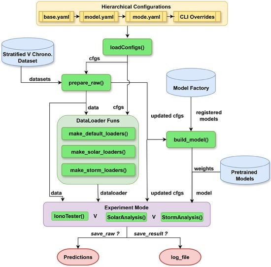
Figure 2.
Testing framework overview.
- Hierarchical configuration: The framework uses a layered configuration stack in the order base →model→mode→ Command Line Interface (CLI). Each layer can be modified independently via YAML or command-line overrides, defining global settings, evaluation mode, and architecture-specific parameters and hyperparameters.
- Model registry and factory: All models in the /source/models/ directory are automatically imported and instantiated based on the configuration. New architectures can be added by creating a Python file in /source/models/ and defining the corresponding configuration in /configs/models/.
- Testing modes and output: Three evaluation modes are supported, namely default testing with IonoTester(), solar intensity-based evaluation with SolarAnalysis(), and geomagnetic storm evaluation with StormAnalysis(). Each run can optionally save predictions or simply log the results.
All individual hyperparameters and model configurations for each architecture are provided on the model repository https://huggingface.co/Mertjhan/IonoBenchv1 (accessed on 10 July 2025).
3.3.2. Metrics
Model performance is assessed using three standard metrics: root mean squared error (RMSE), coefficient of determination (), and structural similarity index measure (SSIM).
- RMSE: Quantifies the average magnitude of prediction error (in TECU).
- : Measures how well the predicted patterns align with overall fluctuations in the ground truth.
- SSIM [41]: Evaluates similarity based on local window statistics while comparing brightness (mean), contrast (variance), and structural consistency (normalized correlation) between predicted and true GIM frames.
Each metric is computed per GIM frame. Overall performance is reported as the mean of all samples and all horizons, with standard deviations included to indicate variability. For horizon-specific performance, the mean and standard deviation are computed across all samples for each forecast horizon.
4. Investigating Future Bias in Stratified Split
A potential drawback of stratified splitting is its violation of temporal order, which may allow the model indirect access to future observations. To assess whether stratified splitting still supports generalization under operational constraints, where future data is unavailable, we compared it against a strictly chronological baseline with matched solar activity coverage.
The valid_v3 subset (a high-activity period; see Figure A2) served as the common evaluation window, as it avoids future data leakage under both splitting strategies. In the chronological setup, the model was trained on data from 2000 to 2016 and validated on data from 2019 to 2023. This configuration matches the training volume of the stratified split and approximates its solar intensity distribution, enabling a fair comparison of the two approaches (see Appendix C, Table A3).
Both configurations were trained with SimVPv2 using an identical pipeline with hyperparameter tuning, as described in Section 3.2, and were evaluated on the held-out valid_v3 subset. As shown in Figure 3 and Table 2, the stratified split shows consistent performance increase over the chronological baseline across all forecast horizons, yielding a lower RMSE and higher .
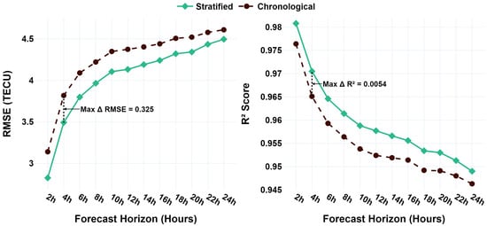
Figure 3.
RMSE and comparison of Stratified vs. Chronological splits across forecast horizons.
Table 2.
Overall performance comparison between Stratified and Chronological splits.
While this comparison focused on a high-activity period, extending the analysis to other solar conditions would require redefining the stratified subsets to maintain balance without introducing data leakage. Such adjustments would compromise the consistency of the comparison and were therefore left outside the scope of this study.
Overall, these results provide encouraging evidence that using a stratified split, despite violating temporal order, may not preclude effective model generalization. However, we must note that for the stratified model, the valid_v3 evaluation data was a subset of the larger validation set used for tuning, which may contribute to this performance margin. Consequently, for final pre-deployment validation, chronological splits remain indispensable to mitigate any potential for future information leakage and ensure true operational generalizability. This aligns with the hybrid development–deployment strategy discussed in Section 6.
5. Results
This section presents a comprehensive evaluation of the benchmarked models using the proposed framework. The analysis begins with overall performance across the full test set with a climatological base reference (IRI 2020), followed by a breakdown of model behavior under varying solar activity levels. It then examines performance during distinct phases of selected geomagnetic storms, incorporating average results across all 16 storms. Further comparison is provided through a visual analysis of a superintense storm versus a quiet-day scenario. The evaluation concludes with a benchmarking of the top-performing model against an operational ionosphere reference (C1PG).
5.1. Overall Performance
Table 3 presents the overall test set performance of the three evaluated models. In addition to accuracy, we report training time and normalized memory usage to account for varying batch sizes due to hardware and tuning constraints.
Table 3.
Overall performance comparison of trained models and the empirical IRI 2020 baseline.
Among the models, SimVPv2 demonstrates the best performance across all metrics, achieving the lowest RMSE (), highest coefficient of determination (), and best structural similarity (). It also shows the lowest performance variance across the test set and completes training faster than the other models under the current configuration.
Interestingly, DCNN, despite being an older and lightweight model, remains highly competitive and slightly outperforms SwinLSTM in every metric. While SwinLSTM has the largest parameter count and memory footprint, these do not yield improved predictive accuracy under the current evaluation conditions.
The IRI 2020 results, derived using default settings and updated drivers, serve as a climatological benchmark across the same test set. With an overall RMSE of TECU (, SSIM = ), the model captures broad TEC patterns. As expected from a monthly median model, its performance underperforms in a test set that is designed to challenge dynamic responses of an ionospheric nature. The performance gap reported is consistent with previous findings that empirical climatologies are outperformed by data-driven models. While IRI remains valuable for climatological reference, its nature limits the model’s responsiveness to real-time solar-terrestrial dynamics. Subsequent analyses omit IRI 2020, as its output is constant across forecast horizons, whereas the remainder of this study focuses on evaluating time-varying AI forecasts and C1PG.
5.2. Performance Across Solar Activity Levels
Evaluating performance across the stratified solar activity classes (Section 2.3) reveals key differences in model robustness. Figure 4a reports the average RMSE per solar class, aggregated across all forecast horizons. Under very weak and weak solar conditions, all models perform similarly to their overall test set rankings, with SimVPv2 achieving the lowest error, followed by DCNN and SwinLSTM.
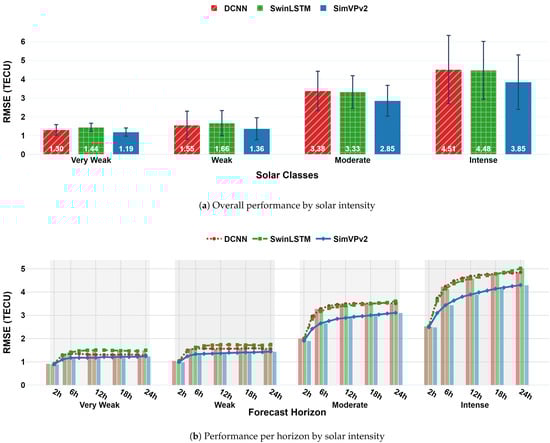
Figure 4.
Solar Analysis.
However, as solar activity intensifies, the relative performance of the models begins to shift. In the moderate and intense solar classes, SwinLSTM performs slightly better than DCNN (reversing the trend seen in weak conditions), and the overall error magnitudes increase substantially. This suggests that DCNN and SwinLSTM may be more sensitive to elevated solar forcing, while SimVPv2 maintains better stability.
Figure 4b provides a horizon-wise breakdown of this trend, showing that all models exhibit rising error over time, especially under higher solar activity levels. Notably, SimVPv2 retains a more gradual error progression, with increasing performance separation from the recurrent models as the forecast horizon lengthens.
5.3. Geomagnetic Storm Analysis
This analysis focuses on the 16 distinct geomagnetic storm events (including 2 superintense storms with Dst dips exceeding nT). Storm windows are extracted using a symmetrical period of ±3 days around the minimum Dst value. Within each window, we define the main phase as the ±6 h interval surrounding the Dst minimum, based on the period of most rapid ionospheric change. This design allows phase-specific error analysis.
5.3.1. RMSE Timeseries for Selected Storms
Figure 5 illustrates model behavior across three storm events from the test set, selected to represent a spectrum of geomagnetic severity: two superintense storms (Dst dips of and ) and one intense, comparatively less severe storm (Dst dip of ). For each storm, the first three columns show the RMSE time series across the full storm window at 2 h, 12 h, and 24 h forecast horizons. The final column summarizes the phase-specific RMSE (commencement, main, recovery) averaged across all horizons, with standard deviations shown as error bars.
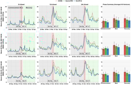
Figure 5.
Forecasted RMSE during geomagnetic storms by phase and horizon.
An analysis of storm phases indicates that forecasting errors peak during the main phase of geomagnetic storms. This is largely due to the rapid development of electric fields and changes in atmospheric winds that disturb ionospheric density and structure in ways that are difficult for models to accurately capture [43,44]. During the recovery phase, errors remain elevated as the ionosphere undergoes a slower return to equilibrium, influenced by lingering effects like altered composition and residual electrodynamic forcing [45].
Across all three storms, distinct model behaviors emerge. DCNN performs relatively well during the commencement phase of storms 2 and 3 but struggles to capture the sharp dynamics of the main and recovery phases, likely due to its simpler recurrent structure. In contrast, SwinLSTM tends to trail DCNN during early phases but shows marked improvements as the phase complexity increases, potentially reflecting its capacity to model temporally evolving structures. Lastly, SimVPv2 demonstrates strong overall stability, but its underperformance during the commencement of storm 2 might suggest storm-specific challenges.
5.3.2. Average Storm-Phase Impact Compared to Quiet Conditions
To complement the event-level storm evaluation, we compute phase-wise RMSE across all 16 storms, averaged across all forecast horizons. For comparison, we define a set of `quiet periods’ by selecting non-storm test samples from the moderate and intense solar intensity levels to isolate the impact of storm conditions from the background solar activity. Furthermore, only samples with Dst values nT are selected. While this range may still contain weak or moderate geomagnetic storms, they are not yet considered in our dataset’s storm classification and are therefore excluded from the storm category in this analysis.
Table 4 presents the RMSE values of each model during quiet periods and across the three storm phases, alongside the corresponding percentage increases relative to quiet-time performance. All models experience the greatest degradation during the main phase, where DCNN and SimVPv2 show over a 140% increase in RMSE relative to quiet conditions. SwinLSTM records a 119.1% increase, indicating a somewhat more stable response under highly disturbed conditions.
Table 4.
Phase-wise RMSE and relative increase during storm periods compared to quiet periods.
Among the models, SimVPv2 achieves the lowest absolute RMSE with TECU during commencement, TECU in the main phase, and TECU in the recovery phases. In contrast, SwinLSTM, although not the most accurate in absolute terms, demonstrates the smallest relative performance loss, with an average increase of 55.8% over the full storm window.
Overall, SimVPv2 is the most accurate model across storm conditions, while SwinLSTM appears to be the most robust in terms of relative degradation. DCNN performs competitively with its SOTA counterpart SwinLSTM, under quiet conditions but exhibits the highest sensitivity to storm-phase dynamics, particularly during the main and recovery periods.
5.3.3. Visual Comparison: Residual Patterns During Stormy vs. Quiet Conditions
Lastly, Figure 6 contrasts performance during two representative scenarios from a period of high solar activity: one during quiet geomagnetic conditions (Dst nT) and one during a superintense storm (Dst nT). With this, we aimed to qualitatively assess spatial performance across contrasting geophysical conditions.
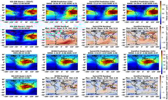
Figure 6.
Prediction and residual map comparisons on stormy and quiet days for DCNN, SwinLSTM, and SimVPv2 models (12 h forecast).
Figure 6 displays 12 h forecast outputs from DCNN, SwinLSTM, and SimVPv2, alongside the corresponding IGS GIM reference maps.
The storm case reflects one of the highest RMSE instances in the test set and offers insight into model behavior under extreme ionospheric disturbance. All models exhibit substantial residuals, with local errors exceeding 40 TECU. Among them, SimVPv2 captures the global TEC distribution most accurately, maintaining lower spatial bias and a more coherent structure across equatorial and mid-latitude regions. In contrast, both DCNN and SwinLSTM struggle in the Southern Hemisphere, where DCNN exhibits a substantial overestimation of TEC at mid-to-high latitudes, while SwinLSTM shows only a slight overestimation. Statistically, DCNN shows the greatest error dispersion (Max: 46.61 TECU, Std: 13.81), while SimVPv2 demonstrates the most compact residual profile (Max: 35.69 TECU, Std: 8.17).
Under quiet conditions, all models perform well, generating visually consistent TEC maps. Their residual patterns are broadly similar, though subtle differences remain. SimVPv2 again records the lowest RMSE ( TECU for this instance) and standard deviation ( TECU), both DCNN and SwinLSTM exhibit elevated positive residuals concentrated near the eastern equatorial region, indicating that these models might be overestimating TEC in this region under quiet conditions. SimVPv2, on the other hand, produces lower residual magnitudes and shows fewer spatial artifacts, suggesting improved consistency in representing quiet-time TEC structures.
5.4. Comparison with C1PG Operational Baseline
Finally, we compare SimVPv2, the top-performing model in our evaluation, against C1PG, a widely used operational reference. C1PG is a 1-day global TEC forecast produced by the CODE analysis center and updated once per day. While several other operational ionospheric models exist [46,47], C1PG remains the predominant baseline in the recent literature due to its ease of access and consistent availability.
This comparison allows us to assess SimVPv2’s performance against a well-established operational standard across different solar activity phases. C1PG has been available since 2014, enabling comparison across the test_v3 (solar low), valid_v2 (solar descent), and valid_v3 (solar high) subsets defined in our framework (Appendix C). Since C1PG provides daily predictions, we post-processed the SimVPv2 outputs into a matching daily format for consistent evaluation. Additionally, C1PG outputs were downsampled to a 2-h cadence to align with the IGS GIM resolution.
Figure 7 presents residual histograms across the three subsets, corresponding to different solar activity levels, and Table 5 summarizes the corresponding performance metrics.
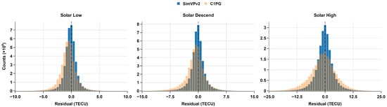
Figure 7.
Residual distributions of TEC predictions for C1PG and SimVPv2 across solar activity phases.
Table 5.
Overall metric comparison between SimVPv2 and C1PG across subsets.
SimVPv2 consistently outperforms C1PG across all the evaluated subsets and metrics. The residual distributions shown in Figure 7 are visibly more compact and symmetric for SimVPv2, especially during periods of elevated solar activity (solar descent and high activity), where C1PG exhibits broader and more asymmetric error tails. Quantitatively, Table 5 confirms SimVPv2’s performance, demonstrating significantly lower RMSE, higher , and higher SSIM values compared to C1PG across all tested activity levels. Notably, SimVPv2 maintains high values (–) across all conditions, while its SSIM score, although consistently higher than C1PG’s, decreases from during low activity to during high activity. This underscores the value of using multiple metrics: confirms the model’s ability to track broad TEC variations, while the SSIM trend reveals that preserving the precise spatial structure of GIMs becomes more challenging under heightened solar activity, even for a high-performing model.
The magnitude of this outperformance is particularly informative. In the demanding high-activity period (valid_v3), SimVPv2 achieves an RMSE approximately 32% lower than C1PG ( vs. TECU). This trend of significant improvement is consistent across all conditions, with a 29% RMSE reduction during solar descent (valid_v2) and a notable 27% reduction during the low-activity period (test_v3). While the valid_v2 and valid_v3 subsets were involved in model tuning, the substantial 27% RMSE reduction on the truly held-out test_v3 subset provides strong evidence of SimVPv2’s generalization capabilities compared to the operational baseline.
6. Discussion
A central insight from this work is the importance of test set composition for evaluating ionospheric models. By stratifying across solar intensity levels and various intense to superintense geomagnetic storms from SC23–SC25, the IonoBench framework allows for evaluating model performance under a wider range of conditions compared to many current studies that focus on narrower testing periods. This stress testing reveals performance degradation during high activity and storms in detail, particularly during the main storm-phase (average RMSE increase >140% vs quiet conditions (Section 5.3.2)). Although a few recent studies incorporate storm phase distinctions [15,18,48,49], phase-specific evaluation remains largely overlooked, even among storm-focused ionospheric modeling works, which typically treat storms as a single block rather than decomposing them into commencement, main, and recovery phases.
Further emphasis should be given to the number and diversity of storms included; as every geomagnetic storm is unique, each can elicit different model responses. For example, in the case of storm 2, SimVPv2’s performance was notably poor during the onset (Section 5.3). Residual pattern analysis revealed that DCNN significantly overestimated TEC in the Southern Hemisphere under certain conditions, whereas SwinLSTM showed only slight overestimation, and SimVPv2 did not exhibit such bias. (Section 5.3.3). Although an aggregate analysis is reported here, the framework and dataset enable deeper, event-specific assessments.
The results of our comparison in Section 4 should be contextualized by the primary motivation for the stratified split. The goal is not simply to achieve better aggregate performance metrics, but to address a crucial methodological pitfall in model evaluation: the risk of performance bias from under-represented extreme events and different conditions. AI-based models often adeptly predict nominal conditions, yet their performance can degrade significantly during critical events like geomagnetic storms. A standard chronological test set may lack a sufficient number of these events, leading to an optimistic assessment of a model’s true operational readiness. While the stratified split excels for this robust testing, the inherent nature of operational deployment favors a chronological approach for final validation. This distinction naturally leads to a practical hybrid approach for model development and deployment. We suggest using a stratified split for benchmarking and comparing different architectures under a wide range of solar and geomagnetic conditions. Once the most robust model is identified, it can then be retrained using a purely chronological split for final deployment. This two-step process ensures the deployed model can operate under realistic, time-respecting conditions while having been validated for generalization across diverse solar–terrestrial conditions.
In terms of modeling architectures, the strong performance of SimVPv2, a non-recurrent convolutional model adapted from general spatiotemporal modeling, highlights the potential for cross-domain architectural transfer into the ionospheric domain. Its success suggests that advancements from fields like video prediction can be effectively leveraged, provided they are adapted and evaluated within a domain-specific context using appropriate benchmarks. This potential strengthens the bridge between ionospheric research and the broader machine learning community, supporting the use of shared benchmarks and modular tools.
At the same time, the results reaffirm the continued relevance of architectures developed specifically for ionospheric modeling. DCNN, despite being an earlier open-source model based on ConvLSTM layers, remained competitive, even outperforming the more complex, Transformer-based SwinLSTM in overall metrics under the tested conditions (Table 3). These results, coupled with the observation that DCNN is rarely compared in recent studies despite its availability, point to a potential issue of knowledge fragmentation and a tendency to overlook existing AI baselines within the field. Maintaining continuity, performing comparisons, and establishing benchmarks are essential for tracking genuine progress and ensuring reproducibility.
The name IonoBench is a conscious reference to WeatherBench, which likewise began with a modest set of models [50] and grew through broader community engagement and follow-up releases [51]. This reflects a shared emphasis on accessibility, transparency, and reproducibility as the foundations of a useful and enduring scientific framework.
While this represents the initial foundation of IonoBench, several limitations are acknowledged. Due to practical constraints such as computational resources, this version includes only three AI baselines, chosen to represent distinct and widely adopted modeling paradigms: convolutional, recurrent, and hybrid architectures. An operational (C1PG) and a climatological (IRI 2020) reference are also included; however, they are not yet integrated into plug-in evaluation protocols, which will be a priority in the near future.
Currently, multichannel inputs are supported, limiting out-of-the-box use for single-channel or scalar models without framework adaptation. Although standard deviations are reported to indicate variability, the framework currently lacks formal uncertainty quantification or metrics specifically evaluating the temporal consistency (smoothness) of forecasts. Additionally, support for explainability tools (e.g., feature attribution, and SHAP value analysis) is not yet integrated.
Future iterations of IonoBench will extend support to a wider range of model architectures, informed by recent developments in the use of Transformers and graph neural networks [24,52,53]. Furthermore, it will also expand the auxiliary input types with magnetic latitude and local time, enhancing the models’ ability to capture geomagnetic field-aligned structures.
Additional priorities include enabling support for scalar and single-channel input models, integrating uncertainty quantification methods, and developing metrics to assess the temporal consistency of forecasts. Improving model interpretability is also a focus, with plans to incorporate explainability tools such as feature attribution and SHAP analysis. These improvements aim to strengthen the scientific and operational utility of the framework. As with similar efforts in other domains, the evolution of IonoBench will be guided by community collaboration, and contributions from researchers are both welcomed and encouraged.
7. Conclusions
This work introduces IonoBench as a building block toward a standardized benchmark for AI-based ionospheric forecasting. It offers an open-source dataset spanning three solar cycles (SC23–SC25) and a modular evaluation platform that incorporates a scientifically motivated stratified split that is solar-balanced and storm-aware. This approach ensures consistent testing across a range of geomagnetic and solar conditions alongside unified preprocessing and evaluation protocols.
Key findings underscore the framework’s value:
- The stratified split enables robust testing across diverse geophysical scenarios, supporting model resilience evaluation under both quiet and storm-time conditions.
- The phase- and event-specific storm analysis reveals performance degradations that are not captured in aggregate metrics, reinforcing the need for detailed storm-aware evaluation.
- Benchmarking diverse architectures reveals that models like SimVPv2 achieve significant improvements over the operational C1PG baseline, with RMSE reductions of approximately 32% (high activity), 29% (solar descent), and 27% on the held-out low-activity test set.
- Comparison with existing open-source baselines (e.g., DCNN) highlights the need for ongoing benchmarking to track progress over time.
Author Contributions
Conceptualization, M.C.T., Y.H.L., and E.L.T.; methodology, M.C.T. and Y.H.L.; software, M.C.T.; validation, M.C.T.; formal analysis, M.C.T.; investigation, M.C.T.; data curation, M.C.T.; writing—original draft preparation, M.C.T.; visualization, M.C.T.; resources, Y.H.L. and E.L.T.; supervision, Y.H.L. and E.L.T.; project administration, Y.H.L. and E.L.T.; funding acquisition, Y.H.L. and E.L.T.; writing—review and editing, M.C.T., Y.H.L., and E.L.T. All authors have read and agreed to the published version of the manuscript.
Funding
This work is funded by Nanyang Technological University (NTU) and Thales Alenia Space.
Data Availability Statement
The IGS GIM and C1PG data are publicly available at https://cddis.nasa.gov/archive/gnss/products/ionex/ (accessed on 10 July 2025). OMNIWeb data can be accessed via https://omniweb.gsfc.nasa.gov/form/dx1.html (accessed on 10 July 2025). The IonoBench benchmark datasets and pretrained models are hosted on Hugging Face repositories at https://huggingface.co/datasets/Mertjhan/IonoBench and https://huggingface.co/Mertjhan/IonoBench, respectively (accessed on 10 July 2025). Source code and accompanying tutorials are provided in the GitHub repository: https://github.com/Mert-chan/IonoBench.git (accessed on 210 July 2025).
Acknowledgments
The authors would like to express their gratitude to Erick Lansard for his valuable guidance and insightful discussions throughout this research. They also wish to thank Yung-Sze Gan, Mathias Vanden Bossche, Sebastien Trilles, and Louis Hecker of Thales Alenia Space for their helpful discussions and support during the course of this work.
Conflicts of Interest
The authors declare no conflicts of interest.
Appendix A. Feature Ablation Study
We conducted a feature ablation study to assess the contribution of different auxiliary input types, using the SimVPv2 model under a fixed experimental setup. OMNI variables were grouped into five categories, as defined in Section 2.1: Solar activity index, geomagnetic indices, SW parameters, IMF components, and time indicators. Each category was removed individually while keeping all others fixed. The results are summarized below in Table A1.
Table A1.
Feature ablation results using SimVPv2.
Table A1.
Feature ablation results using SimVPv2.
| Configuration | RMSE (TECU) | SSIM | |
|---|---|---|---|
| All Features | 2.2523 | 0.9623 | 0.9688 |
| No Solar Activity | 2.4098 | 0.9557 | 0.9644 |
| No Geomagnetic | 2.3945 | 0.9571 | 0.9648 |
| No Solar Wind | 2.3618 | 0.9581 | 0.9658 |
| No IMF | 2.3827 | 0.9568 | 0.9650 |
| No Time | 2.3435 | 0.9588 | 0.9658 |
Bolded values indicate the best performance across configurations.
Excluding the solar activity index () leads to the greatest performance drop, confirming its dominant role in TEC variability. Geomagnetic inputs are the next most impactful, reflecting the test set’s emphasis on storm periods. While individual models may depend more heavily on specific input features, providing access to the full feature set supports robust generalization and ensures fair model comparison.
Appendix B. Data Cleaning
Appendix B.1. IGS GIM Data (IONEX Format)
The IGS GIM dataset presented challenges related to structural inconsistencies and anomalous TEC values. They were addressed as follows:
- 1.
- Structural integrity check: Initial parsing flagged a small number of files with format errors, such as merged digits leading to incorrect row lengths. These were auto-corrected to maintain consistent 71 × 73 grid dimensions.
- 2.
- Extreme TEC outlier filtering: A two-stage filtering process was used to detect physically unrealistic values:
- -
- Global filtering: Maps with values exceeding a dynamic threshold (based on map-level mean and standard deviation) were flagged for large-scale anomalies.
- -
- Local filtering: A sliding-window method with adaptive thresholds (adjusted by latitude) identified localized outliers, accounting for natural TEC variability near the geomagnetic equator.
- 3.
- Correction methods: Global anomalies were corrected via one-dimensional interpolation (latitude or longitude). Local gaps and residual outliers were filled with two-dimensional scattered interpolation and refined using localized median filtering.
- 4.
- Manual verification: The 200 maps with the highest RMS changes post-correction were visually inspected. While minor artifacts may remain at high latitudes, the automated pipeline effectively removed severe outliers.Examples are shown below in Figure A1.

Figure A1.
Examples illustrating the effect of the outlier correction procedure on selected GIMs. Each pair displays the original (left) and corrected (right).
Appendix B.2. OMNIWeb Auxiliary Data Imputation
Missing entries in the OMNIWeb dataset, indicated by standard fill values (e.g., 9999.9, 999.9, 99.99, depending on the parameter), were imputed using a tiered temporal strategy:
- If both the preceding and succeeding values for a parameter were valid, the missing entry was replaced by their average.
- If only one neighboring value (either preceding or succeeding) was valid, that value was used to fill the gap (forward or backward fill).
- If both neighboring values were missing, the gap was filled by sampling from a normal distribution characterized by the mean and standard deviation calculated from all available valid entries for that specific parameter across the entire dataset period.
This approach aimed to preserve temporal continuity while robustly handling data gaps of varying lengths in the auxiliary time series.
Appendix C. Data Split Details
Table A2.
Stratified dataset splits used for model training, validation, and testing. Each subset corresponds to a distinct phase of solar activity.
Table A2.
Stratified dataset splits used for model training, validation, and testing. Each subset corresponds to a distinct phase of solar activity.
| Subset | Start Time | End Time | Solar Activity Phase |
|---|---|---|---|
| train_v1 | 2000-01-01 00:00 | 2000-12-28 22:00 | Ascending |
| test_v1 | 2001-01-01 00:00 | 2001-12-28 22:00 | High Activity |
| train_v2 | 2002-01-01 00:00 | 2007-12-28 22:00 | Descending |
| valid_v1 | 2008-01-01 00:00 | 2008-12-28 22:00 | Low Activity |
| train_v3 | 2009-01-01 00:00 | 2011-12-28 22:00 | Ascending |
| test_v2 | 2012-01-01 00:00 | 2012-12-28 22:00 | Ascending |
| train_v4 | 2013-01-01 00:00 | 2015-10-28 22:00 | High Activity |
| valid_v2 | 2015-11-01 00:00 | 2017-09-05 22:00 | Descending (Solar Descent) |
| train_v5 | 2017-09-08 00:00 | 2018-12-28 22:00 | Low Activity |
| test_v3 | 2019-01-01 00:00 | 2020-09-28 22:00 | Low Activity |
| train_v6 | 2020-10-01 00:00 | 2023-09-26 22:00 | Ascending |
| valid_v3 | 2023-09-30 00:00 | 2024-09-09 00:00 | High Activity |
Bolded subsets indicate the periods used in the comparative evaluation in Section 5.4. Please note one test date (16 June 2019) in the Solar Low subset was excluded due to missing C1PG data.

Figure A2.
Subset identification for stratified and chronological splits, highlighting the distribution of training, validation, and test periods across Solar Cycles 23–25.
Table A3.
Comparison of stratified and chronological splits by dataset size and solar intensity distribution.
Table A3.
Comparison of stratified and chronological splits by dataset size and solar intensity distribution.
| Split | Subset | Total Samples | Solar Intensity Classes 1 |
|---|---|---|---|
| Stratified | Train | 74,904 | 7,368/29,676/23,773/14,087 |
| Valid | 16,597 | 3,864/7,212/2,592/2,929 | |
| Chronological | Train | 74,532 | 7,800/26,748/25,453/14,531 |
| Valid | 17,737 | 2,676/7,644/4,416/3,001 |
1 Ordered as very weak/weak/moderate/intense.
The total number of samples was intentionally matched across splits to ensure a fair and controlled comparison between the stratified and chronological configurations, as shown in Figure A2.
References
- Morton, Y.J.; Yang, Z.; Breitsch, B.; Bourne, H.; Rino, C. Ionospheric Effects, Monitoring, and Mitigation Techniques. In Position, Navigation, and Timing Technologies in the 21st Century, 1st ed.; Wiley: Hoboken, NJ, USA, 2020; Volume 1, pp. 879–937. [Google Scholar] [CrossRef]
- Tsagouri, I.; Belehaki, A.; Themens, D.R.; Jakowski, N.; Fuller-Rowell, T.; Hoque, M.M.; Nykiel, G.; Miloch, W.J.; Borries, C.; Morozova, A.; et al. Ionosphere variability I: Advances in observational, monitoring and detection capabilities. Adv. Space Res. 2023, 72, 5598. [Google Scholar] [CrossRef]
- Heh, D.Y.; Murti, D.S.; Tan, E.L.; Poh, E.K.; Ling, K.V.; Guan, Y.L. Ionospheric Scintillation of GPS Microwave Signals in Singapore. In Proceedings of the Asia-Pacific Microwave Conference (APMC 2014), Sendai, Japan, 4–7 November 2014; pp. 1390–1392. [Google Scholar]
- Heh, D.Y.; Murti, D.S.; Tan, E.L.; Poh, E.K.; Ling, K.V.; Tang, J. Equatorial ionospheric scintillation of BeiDou Navigation Satellite System observed in Singapore. In Proceedings of the ION Pacific PNT Meeting, Honolulu, HI, USA, 20–23 April 2015; pp. 17–24. [Google Scholar]
- Yasyukevich, Y.V.; Zatolokin, D.; Padokhin, A.; Wang, N.; Nava, B.; Li, Z.; Yuan, Y.; Yasyukevich, A.; Chen, C.; Vesnin, A. Klobuchar, NeQuickG, BDGIM, GLONASS, IRI-2016, IRI-2012, IRI-Plas, NeQuick2 and GEMTEC ionospheric models: A comparison in total electron content and positioning domains. Sensors 2023, 23, 4773. [Google Scholar] [CrossRef]
- Liu, L.; Wan, W.; Chen, Y.; Le, H. Solar activity effects of the ionosphere: A brief review. Chin. Sci. Bull. 2011, 56, 1202–1211. [Google Scholar] [CrossRef]
- Kumar, S.; Tan, E.L.; Razul, S.G.; See, C.M.S.; Siingh, D. Validation of the IRI-2012 model with GPS-based ground observation over a low-latitude Singapore station. Earth Planets Space 2014, 66, 17. [Google Scholar] [CrossRef]
- Kumar, S.; Tan, E.L.; Murti, D.S. Impacts of solar activity on performance of the IRI-2012 model predictions from low to mid latitudes. Earth Planets Space 2015, 67, 42. [Google Scholar] [CrossRef]
- Bilitza, D.; Pezzopane, M.; Truhlik, V.; Altadill, D.; Reinisch, B.W.; Pignalberi, A. The International Reference Ionosphere model: A review and description of an ionospheric benchmark. Rev. Geophys. 2022, 60, e2022RG000792. [Google Scholar] [CrossRef]
- Radicella, S.M.; Leitinger, R. The NeQuick model genesis, uses and evolution. Ann. Geophys. 2009, 52, 417–422. [Google Scholar] [CrossRef]
- Maute, A. Thermosphere–ionosphere–electrodynamics general circulation model for the Ionospheric Connection Explorer: TIEGCM-ICON. Space Sci. Rev. 2017, 212, 523–551. [Google Scholar] [CrossRef]
- Huba, J.D.; Joyce, G.; Fedder, J.A. SAMI2 is another model of the ionosphere (SAMI2): A new low-latitude ionosphere model. J. Geophys. Res. Space Phys. 2000, 105, 23035–23053. [Google Scholar] [CrossRef]
- Kaselimi, M.; Voulodimos, A.; Doulamis, N.; Doulamis, A.; Delikaraoglou, D. A causal long short-term memory sequence-to-sequence model for TEC prediction using GNSS observations. Remote Sens. 2020, 12, 1354. [Google Scholar] [CrossRef]
- Kim, J.; Kwak, Y.; Kim, Y.; Moon, S.; Jeong, S.; Yun, J. Potential of regional ionosphere prediction using a long short-term memory deep-learning algorithm specialized for geomagnetic storm period. Space Weather 2021, 19, e2021SW002741. [Google Scholar] [CrossRef]
- Adolfs, M.; Hoque, M.M.; Shprits, Y.Y. Storm-time relative total electron content modelling using machine-learning techniques. Remote Sens. 2022, 14, 6155. [Google Scholar] [CrossRef]
- Yang, J.; Huang, W.; Xia, G.; Zhou, C.; Chen, Y. Operational forecasting of global ionospheric TEC maps 1-, 2- and 3-day in advance by ConvLSTM model. Remote Sens. 2024, 16, 1700. [Google Scholar] [CrossRef]
- Schrijver, C.J.; Kauristie, K.; Aylward, A.D.; Denardini, C.M.; Gibson, S.E.; Glover, A.; Gopalswamy, N.; Grande, M.; Hapgood, M.; Heynderickx, D.; et al. Understanding space weather to shield society: A global road map for 2015–2025 commissioned by COSPAR and ILWS. Adv. Space Res. 2015, 55, 2745–2807. [Google Scholar] [CrossRef]
- Ren, X.; Zhao, B.; Ren, Z.; Wang, Y.; Xiong, B. Deep learning-based prediction of global ionospheric TEC during storm periods: Mixed CNN-BiLSTM method. Space Weather 2024, 22, e2024SW003877. [Google Scholar] [CrossRef]
- Boulch, A.; Cherrier, N.; Castaings, T. Ionospheric activity prediction using convolutional recurrent neural networks. arXiv 2018, arXiv:cs.LG/1810.13273. [Google Scholar] [CrossRef]
- Liu, L.; Morton, Y.J.; Liu, Y. Machine-learning prediction of global ionospheric TEC maps. Space Weather 2022, 20, e2022SW003135. [Google Scholar] [CrossRef]
- Gao, X.; Yao, Y. A storm-time ionospheric TEC model with multichannel features by the spatiotemporal ConvLSTM network. J. Geod. 2023, 97, 9. [Google Scholar] [CrossRef]
- Liu, H.; Wang, H.; Le, H.; Yuan, J.; Shan, W.; Wu, Y.; Chen, Y. CGAOA-STRA-BiConvLSTM: An automated deep learning framework for global TEC map prediction. GPS Solut. 2025, 29, 55. [Google Scholar] [CrossRef]
- Tsagouri, I.; Themens, D.R.; Belehaki, A.; Shim, J.S.; Hoque, M.M.; Nykiel, G.; Borries, C.; Morozova, A.; Barata, T.; Miloch, W.J. Ionosphere variability II: Advances in theory and modeling. Adv. Space Res. 2023, 72, 6051. [Google Scholar] [CrossRef]
- Yu, F.; Yuan, H.; Chen, S.; Luo, R.; Luo, H. Graph-enabled spatio-temporal transformer for ionospheric prediction. GPS Solut. 2024, 28, 203. [Google Scholar] [CrossRef]
- Zhang, R.; Li, H.; Shen, Y.; Yang, J.; Li, W.; Zhao, D.; Hu, A. Deep learning applications in ionospheric modeling: Progress, challenges, and opportunities. Remote Sens. 2025, 17, 124. [Google Scholar] [CrossRef]
- Tan, C.; Huang, Z.; Zhang, X.; Zhang, Q.; Zhang, M.; Li, S.Z. OpenSTL: A comprehensive benchmark for spatio-temporal forecasting. arXiv 2023, arXiv:cs.LG/2306.11249. [Google Scholar]
- Tang, S.; Li, C.; Zhang, P.; Tang, R. SwinLSTM: Improving spatiotemporal prediction accuracy using Swin Transformer and LSTM. arXiv 2023, arXiv:cs.LG/2308.09891. [Google Scholar]
- Tan, C.; Gao, Z.; Li, S.; Li, S.Z. SimVPv2: Towards simple yet powerful spatiotemporal predictive learning. arXiv 2024, arXiv:cs.CV/2211.12509. [Google Scholar] [CrossRef]
- Chen, S.; Athreyas, K.B.N.; Lansard, E.; di Milano, P. Orbit Manoeuvre Strategies for Very Low Earth Orbit (VLEO) Satellites under Solar Activity and Drag Effects. J. Br. Interplanet. Soc. 2024, 77, 223–228. [Google Scholar] [CrossRef]
- Hernández-Pajares, M.; Juan, J.M.; Sanz, J.; Orus, R.; Garcia-Rigo, A.; Feltens, J.; Komjathy, A.; Schaer, S.C.; Krankowski, A. The IGS VTEC maps: A reliable source of ionospheric information since 1998. J. Geod. 2009, 83, 263–275. [Google Scholar] [CrossRef]
- King, J.H.; Papitashvili, N.E. Solar wind spatial scales and comparisons of hourly Wind and ACE plasma and magnetic field data. J. Geophys. Res. 2005, 110, 2004JA010649. [Google Scholar] [CrossRef]
- Turkmen, M.; Lee, Y.H.; Tan, E.L. Correlation of solar and geomagnetic indices during Solar Cycle 24 with TEC-derived metrics. In Proceedings of the 2024 IEEE AP-S/URSI Symposium, Florence, Italy, 14–19 July 2024; pp. 1445–1446. [Google Scholar]
- Guyon, I.; Elisseeff, A. An introduction to variable and feature selection. J. Mach. Learn. Res. 2003, 3, 1157–1182. [Google Scholar] [CrossRef][Green Version]
- Wang, S.; Huang, S. Quantify the information contributions of external drivers to global ionospheric TEC. J. Geophys. Res. Space Phys. 2023, 128, e2023JA031897. [Google Scholar] [CrossRef]
- Gonzalez, W.D.; Joselyn, J.A.; Kamide, Y.; Kroehl, H.W.; Rostoker, G.; Tsurutani, B.T.; Vasyliunas, V.M. What is a geomagnetic storm? J. Geophys. Res. 1994, 99, 5771–5792. [Google Scholar] [CrossRef]
- Gonzalez, W.D.; Tsurutani, B.T.; Lepping, R.P.; Schwenn, R. Interplanetary phenomena associated with very intense geomagnetic storms. J. Atmos. Sol.-Terr. Phys. 2002, 64, 173–181. [Google Scholar] [CrossRef]
- Gonzalez, W.D.; Echer, E.; Clúa De Gonzalez, A.L.; Tsurutani, B.T.; Lakhina, G.S. Extreme geomagnetic storms, recent Gleissberg cycles and space era-superintense storms. J. Atmos. -Sol.-Terr. Phys. 2011, 73, 1447–1453. [Google Scholar] [CrossRef]
- Tang, J.; Li, Y.; Ding, M.; Liu, H.; Yang, D.; Wu, X. An ionospheric TEC forecasting model based on a CNN-LSTM-attention mechanism neural network. Remote Sens. 2022, 14, 2433. [Google Scholar] [CrossRef]
- Tang, J.; Zhong, Z.; Hu, J.; Wu, X. Forecasting regional ionospheric TEC maps over China using BiConvGRU deep learning. Remote Sens. 2023, 15, 3405. [Google Scholar] [CrossRef]
- Williams, R.J.; Zipser, D. A learning algorithm for continually running fully recurrent neural networks. Neural Comput. 1989, 1, 270–280. [Google Scholar] [CrossRef]
- Wang, Z.; Bovik, A.C.; Sheikh, H.R.; Simoncelli, E.P. Image quality assessment: From error visibility to structural similarity. IEEE Trans. Image Process. 2004, 13, 600–612. [Google Scholar] [CrossRef]
- Bidula, V. iricore: Python Interface to IRI-2016 and IRI-2020, 2024. Version 1.9.0. Available online: https://iricore.readthedocs.io (accessed on 3 June 2025).
- Lu, G.; Zakharenkova, I.; Cherniak, I. Large-scale ionospheric disturbances during the 17 March 2015 storm: A model-data comparative study. J. Geophys. Res. Space Phys. 2020, 125. [Google Scholar] [CrossRef]
- Balan, N.; Shiokawa, K.; Otsuka, Y. A physical mechanism of positive ionospheric storms at low latitudes and midlatitudes. J. Geophys. Res.: Space Phys. 2010, 115. [Google Scholar] [CrossRef]
- Balan, N.; Otsuka, Y.; Nishioka, M.; Liu, J.Y. Physical mechanisms of the ionospheric storms at equatorial and higher latitudes during the recovery phase of geomagnetic storms. J. Geophys. Res. Space Phys. 2013, 118, 2660–2669. [Google Scholar] [CrossRef]
- Aragon-Angel, A.; Zürn, M.; Rovira-Garcia, A. Galileo ionospheric correction algorithm: An optimization study of NeQuick-G. Radio Sci. 2019, 54, 1156–1169. [Google Scholar] [CrossRef]
- Codrescu, M.V.; Negrea, C.; Fedrizzi, M.; Fuller-Rowell, T.J.; Dobin, A.; Jakowsky, N.; Khalsa, H.; Matsuo, T.; Maruyama, N. A real-time run of the coupled thermosphere ionosphere plasmasphere electrodynamics (CTIPe) model. Space Weather 2012, 10, S02001. [Google Scholar] [CrossRef]
- Ren, X.; Yang, P.; Mei, D.; Liu, H.; Xu, G.; Dong, Y. Global ionospheric TEC forecasting for geomagnetic storm time using a deep learning-based multi-model ensemble method. Space Weather 2023, 21, e2022SW003231. [Google Scholar] [CrossRef]
- Ren, X.; Zhao, B.; Ren, Z.; Xiong, B. Ionospheric TEC prediction in China during storm periods based on deep learning: Mixed CNN-BiLSTM method. Remote Sens. 2024, 16, 3160. [Google Scholar] [CrossRef]
- Rasp, S.; Dueben, P.D.; Scher, S.; Weyn, J.A.; Mouatadid, S.; Thuerey, N. WeatherBench: A benchmark dataset for data-driven weather forecasting. J. Adv. Model. Earth Syst. 2020, 12, e2020MS002203. [Google Scholar] [CrossRef]
- Rasp, S.; Dueben, P.D.; Scher, S.; Weyn, J.A.; Mouatadid, S.; Thuerey, N. WeatherBench 2: A benchmark for the next generation of data-driven global weather models. arXiv 2024, arXiv:cs.LG/2308.15560. [Google Scholar] [CrossRef]
- Wang, H.S.; Jwo, D.J.; Lee, Y.H. Transformer-based ionospheric prediction and explainability analysis for enhanced GNSS positioning. Remote Sens. 2024, 17, 81. [Google Scholar] [CrossRef]
- Liu, R.; Jiang, Y. Ionospheric VTEC maps forecasting based on graph neural network with transformers. IEEE J. Sel. Top. Appl. Earth Obs. Remote Sens. 2025, 18, 1802–1816. [Google Scholar] [CrossRef]
Disclaimer/Publisher’s Note: The statements, opinions and data contained in all publications are solely those of the individual author(s) and contributor(s) and not of MDPI and/or the editor(s). MDPI and/or the editor(s) disclaim responsibility for any injury to people or property resulting from any ideas, methods, instructions or products referred to in the content. |
© 2025 by the authors. Licensee MDPI, Basel, Switzerland. This article is an open access article distributed under the terms and conditions of the Creative Commons Attribution (CC BY) license (https://creativecommons.org/licenses/by/4.0/).