Abstract
Vegetation photosynthesis is a key Earth system process that can fix carbon dioxide in the atmosphere. Mountainous areas usually have high productivity and extensive vegetation cover, but their study requires a higher spatiotemporal resolution due to the complex climate and vegetation variations with altitude. In this study, we analyzed the variations and climatic responses of vegetation gross primary productivity (GPP) in northwestern Hubei, China, at a 30 m spatial resolution from 2001 to 2020, based on the fusion of multi-source remote sensing data. A GPP estimation framework based on the CASA model was applied, and spatiotemporal fusion of Landsat and MODIS data was achieved using the STNLFFM algorithm. The results indicate that GPP exhibits higher values in the mountainous regions of west Shennongjia, compared to the eastern plain regions, with a generally increasing trend with increasing elevation. GPP has shown an overall increasing trend over the past 20 years, with almost 90% of the high-elevation regions showing an increasing trend, and the low-elevation regions showing an opposite trend. The relationship between GPP and climate factors is greatly impacted by the temporal scale, with the most pronounced correlation at a seasonal scale. The impact of temperature has been generally stable over the past 20 years across different altitudes, while the relationship with precipitation has exhibited an overall decreasing trend with the increase of altitude. Precipitation and temperature correlations show opposing variations in different months and elevations, which can be mainly attributed to the varied climatic conditions in the different elevations.
1. Introduction
Vegetation is the key component of terrestrial ecosystems that can balance the global carbon cycle by absorbing carbon dioxide (CO2) and releasing oxygen (O2) through photosynthesis. As a result, vegetation photosynthesis is a critical Earth process for reducing greenhouse gases in the atmosphere and the mitigation of global climate change [1,2,3,4]. With the background of dramatic global change, it is essential to understand the variations and driving factors of vegetation photosynthesis [5]. Gross primary productivity (GPP), which is the total amount of carbon fixed by plants in a given period of time, reflects the ability of ecosystem productivity and carbon sequestration. As a result, it is meaningful to monitor the changes and responses of GPP as it is a key indicator for understanding the global carbon cycle and combating climate change [6,7,8]. Recent studies have highlighted that climate variability plays a dominant role in driving changes in GPP [9,10]. In these studies, remote sensing data have played an essential role by providing consistent, large-scale, and high-resolution observations that enable the detailed assessment of vegetation responses to climatic factors across diverse and complex landscapes. Nevertheless, accurately capturing the influence of climate variability on GPP at fine spatiotemporal scales remains a significant challenge, especially in heterogeneous and mountainous regions where environmental conditions vary sharply over short distances.
Traditionally, methods for obtaining GPP can be broadly categorized into two main types: site observation-based methods and model simulation-based methods [8]. Site observation-based methods, such as eddy covariance (EC) methods, directly measure the ecosystem carbon fluxes, which can provide site-level GPP with high precision, but their application is usually limited by the spatial and temporal resolution [11]. Model simulation-based methods are the mainstream methods for global or large-scale GPP applications. With the advancement of remote sensing technology, various remote sensing-driven models have been developed, which are better suited for large-scale applications. Remote sensing techniques can be used to calculate vegetation indices through the combination of different spectral bands. Examples of vegetation indices are the normalized difference vegetation index (NDVI) and the enhanced vegetation index (EVI). Various structural and functional parameters of vegetation can also be derived, including the leaf area index (LAI), leaf chlorophyll content (LCC), and maximum rate of carboxylation (Vcmax). These parameters are the fundamental drivers for many models, which can be primarily divided into statistical models, process models, and light use efficiency (LUE) models [12]. Among the different models, statistical models usually show accuracy limitations due to their simple basis and lack of mechanism [13], and process models typically suffer from a complex model structure and numerous parameters, despite being developed based on a strong theoretical foundation and clear mechanism [14]. As a result, LUE models have become the most widely applied models, due to their clear LUE principles, computational simplicity, and suitability for regional- and global-scale estimation when combined with remote sensing data [15].
Based on these methods, a large number of large-scale GPP estimation and analysis studies have been conducted to understand the changes and driving factors for regional or global vegetation photosynthesis. Not only have the spatial distribution and temporal variation trends of GPP been well analyzed, but the response of GPP to different climatic factors, extreme climatic events, and various disturbances has been extensively studied. There have also been many studies of specific sensitive areas, which can help provide recommendations for conservation policies [16,17,18,19,20]. However, these studies have mainly focused on large regions, and the specific conditions and characteristics in complex mountainous areas have still not been well investigated. Compared to plain regions, mountainous regions exhibit diverse slopes, aspects, and elevation changes, even over small areas, which makes the climate and vegetation distribution much more complex. On the one hand, due to the vertical zonation, vegetation shows strong spatial heterogeneity, with the rich species showing different variation trends and responses to climate change, even in a small region [21]. On the other hand, climatic factors also vary significantly with elevation; for example, temperature decreases with increasing elevation, and the moisture from precipitation may not be easily retained in high-altitude areas, leading to pronounced climatic differentiation [22,23,24]. Consequently, the response of photosynthesis to environmental conditions is more complex in mountainous regions [25], and data with a finer spatiotemporal resolution are also required to represent the sharply varied GPP and climatic conditions.
Although there are many sensors that can obtain observations supporting GPP estimation at various resolutions, they all have their unique strengths and limitations, which results in it being difficult to fulfill the demand for GPP studies in mountainous regions. For example, Moderate-Resolution Imaging Spectroradiometer (MODIS) products feature spatial resolutions of 500 m or 1000 m with daily observations, enabling consistent monitoring. However, their coarser resolution often misses fine-scale details, especially in complex terrain such as mountainous regions, where subtle changes can be difficult to detect [23]. Conversely, Landsat sensors feature a 30 m spatial resolution, capturing detailed landscape variations. However, their 16-day revisit cycle and cloud cover issues limit the generation of continuous, cloud-free time series. Similarly, the Sentinel series of satellites, with resolutions as fine as 10 m and diverse multi-sensor capabilities, supports many applications across various fields. Nonetheless, Sentinel data faced the problems of cloud contamination and insufficient temporal resolution, hindering the generation of seamless time series. To address these issues, integrating the complementary strengths of the different sensors is vital. Multi-source remote sensing fusion combines the high temporal resolution of sensors such as MODIS with the fine spatial detail of Landsat. Studies have shown that this approach can improve data accuracy, enhance coverage, and provide robust datasets for monitoring complex, climatically variable regions [26,27,28,29]. Multi-source remote sensing fusion excels in applications needing precise temporal sequences and fine-scale change detection, such as land use monitoring. Combining the high spatial resolution of Landsat data with the high temporal resolution of MODIS data better captures vegetation dynamics in complex mountainous terrain. This fusion allows us to overcome the limitations of using either dataset alone and provides a more accurate assessment of GPP variations. Thus, multi-source data fusion was central to this study.
Northwestern Hubei is one of the most important ecological zones in central China, with a high forest coverage rate and complex environments. The topography is particularly complex in the region, with the elevation ranging from 42 m to 3103 m. The core area, Shennongjia Forestry District, shows an elevation difference over 2700 m, only covering a 3253 km2 region. This unique topographic setting supports 3767 vascular plant species, and features 11 vegetation types across a complete altitudinal spectrum from low to high elevations. The rich biodiversity makes it critically important to research the changes in vegetation in this region, which also supports its recognition as the first site in China to be simultaneously recognized under three major global conservation designations. Shennongjia is also the only administrative region in China named after a forest area, as a key national nature reserve featuring well-preserved primeval forests and key ecological functional zones. Northwestern Hubei is a transitional zone from subtropical to temperate climate; however, due to the great elevation differences, the precipitation and temperature also show obvious spatial heterogeneity, with the regions at higher altitudes showing lower temperatures and receiving more precipitation, which favors forest growth. In this condition, the distribution of vegetation is also shaped by the vertical zonation and climatic gradients, making its distribution exhibit strong spatial heterogeneity [30,31,32,33,34]. As a result, it is of great significance to study the variations and responses of vegetation photosynthesis in northwestern Hubei with complex mountainous topography. Although many previous studies have reached many conclusions on vegetation diversity and distribution in Shennongjia due to its high biodiversity, the distribution and variations in vegetation photosynthetic carbon sequestration still remain poorly understood and deserve further investigation [35,36,37].
Thus, in this study, we targeted northwestern Hubei, using high-resolution remote sensing imagery from multiple sources, regional meteorological data, and land cover data, employing an LUE model to estimate regional GPP. We further integrated a digital elevation model (DEM) and meteorological data to systematically analyze the spatiotemporal trends and driving factors of GPP, aiming to reveal the dynamic characteristics and driving mechanisms of vegetation carbon sequestration, thereby enriching the theoretical research on this topic in the region. The spatiotemporal trends and driving factors of GPP were also systematically analyzed across different time scales and elevations. In addition, GPP was estimated using the CASA model, and cross-validation was performed with MODIS GPP and GOSIF GPP products to evaluate the reliability and consistency of the results.
2. Materials and Methods
2.1. Study Area
As shown in Figure 1, northwestern Hubei is located in the northwest of Hubei province, at the junction of Hubei, Henan, Shaanxi, and Chongqing provinces. It forms the heartland of the Qinba Mountains in the middle reaches of the Han River, encompassing the Shennongjia Forest District, the entire city of Shiyan, most of the city of Xiangfan (including Danjiangkou, Baokang, Gucheng, and Nanzhang), and parts of the city of Yichang (Yuan’an).
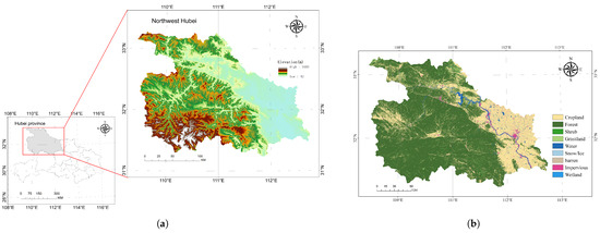
Figure 1.
Study area and elevation distribution for northwestern Hubei. (a) Location of northwestern Hubei in Hubei province and its elevation distribution. (b) Land cover of northwestern Hubei.
Situated on the northern edge of the subtropics, this region falls within the mid-latitude northern subtropical monsoon climate zone. The average annual temperature is approximately 15 °C, with an annual effective accumulated temperature of 4878.4 °C for temperatures ≥ 10 °C. The average annual relative humidity is 73.7%, and the mean annual precipitation is around 800 mm. In the mountainous areas of the region, precipitation often exceeds 1000 mm annually. Precipitation is predominantly concentrated in summer, accounting for 40–50% of the yearly total, while winter sees the least, at about 5%. Consequently, precipitation distribution is uneven throughout the year, and the climate is characterized by distinct seasons, long winters, short summers, rapid warming in spring, swift cooling in autumn, abundant summer precipitation, and minimal rain or snow in winter. These climatic conditions foster rich habitats and biodiversity, making northwestern Hubei a key area of concentrated forest distribution in Hubei province. The region is also home to the highest number of nature reserves in the province.
2.2. Study Data
In this study, we integrated multiple datasets to investigate vegetation photosynthesis and carbon sequestration in northwestern Hubei from 2001 to 2020 (as shown in Table 1). Remote sensing data, including Landsat surface reflectance data and MOD13Q1 NDVI data, were utilized to derive high-resolution NDVI for GPP estimation, capturing fine-scale vegetation dynamics. Climate data from ERA5, reprocessed to a 16-day resolution, provided the essential meteorological inputs for the LUE model, enabling the analysis of the environmental influences on GPP. GPP products, including the Global OCO-2 SIF-based GPP (GOSIF) and MODIS GPP products, served as the control groups for cross-validation, ensuring the reliability of the estimated GPP. In addition, the China Land Cover Dataset (CLCD) supported the derivation of key parameters such as the maximal sampling rate (SRmax) and LUE, while the Copernicus GLO-30 DEM was used in the elevation-based analysis, addressing the complex topography of the study region. The integration of multi-source datasets allowed us to leverage the strengths of different sensors and data types—such as the high spatial resolution of Landsat, the high temporal frequency of MODIS, and the comprehensive climate coverage of ERA5—thus enhancing both the spatial and temporal representativeness of the GPP estimation and improving the robustness of our analysis in complex mountainous environments.

Table 1.
Data specifications for the remote sensing, climate, and GPP products used in this study.
2.2.1. Remote Sensing Data
The surface reflectance data used in this study were sourced from the Landsat surface reflectance dataset provided by the United States Geological Survey (USGS), with a spatial resolution of 30 m. The choice of Landsat data is due to their relatively high spatial resolution, which allows for better capture of fine-scale variations in mountainous regions. Based on the temporal coverage, the dataset includes Landsat 5, Landsat 7, and Landsat 8 data. Cloud-free images with path/row numbers (124, 38), (125, 37), (125, 38), (126, 37), and (126, 38) were selected from 2001 to 2020 (https://earthexplorer.usgs.gov/ (accessed on 1 November 2024)). The data were downloaded as surface reflectance data. After the mosaicking and clipping process, a total of 80 scenes were obtained quarterly, covering the whole of northwestern Hubei.
The Landsat surface reflectance data were processed through band math operations to derive the Landsat NDVI data. The NDVI was calculated as follows:
where represents the near-infrared band, and represents the red band.
Due to it being difficult to form time series with Landsat data, MODIS NDVI data were also applied and fused with the Landsat data. The selected NDVI product was MOD13Q1 (available at https://modis.gsfc.nasa.gov/data/dataprod/mod13.php (accessed on 1 November 2024)), with a temporal resolution of 16 days and a spatial resolution of 250 m, covering the period from 2001 to 2020. This dataset comprises 460 scenes with tile number h27v05.MODIS data offering a higher temporal resolution (16-day composite) and are relatively less affected by cloud contamination, which makes them well-suited for constructing continuous and consistent time series. After clipping and filtering, the MODIS NDVI data for northwestern Hubei were obtained.
2.2.2. Climate Data
The climate data used in this study were sourced from ERA5 post-processed daily statistics on single levels from 1940 to the present (https://cds.climate.copernicus.eu/datasets/derived-era5-single-levels-daily-statistics?tab=download (accessed on 1 March 2025)), with a spatial resolution of 0.5∘ × 0.5∘. This globally available dataset provides daily temporal resolution, allowing for detailed characterization of climate variability over time. These data were synthesized from a daily temporal resolution to a 16-day resolution, where the clear-sky direct solar radiation at the surface and the surface solar radiation downwards were combined into total radiation. The climate data were also reprojected, resampled, and clipped to align with the Landsat NDVI data, preparing the data for GPP estimation using the LUE model.
2.2.3. GPP Products
The GOSIF GPP [38] (https://globalecology.unh.edu/data/GOSIF-GPP.html (accessed on 1 March 2025)) and MODIS GPP (https://modis.gsfc.nasa.gov/data/dataprod/mod17.php (accessed on 1 March 2025)) products were selected as control datasets for cross-validation. GOSIF-GPP is a global high-resolution GPP dataset derived from solar-induced chlorophyll fluorescence (SIF), which directly reflects photosynthetic activity and provides high sensitivity to GPP [38]. MODIS GPP is based on an LUE model driven by vegetation indices and meteorological data from the MODIS sensor. Although less physiologically direct, it offers a long-term, globally consistent GPP record and is widely used in carbon and climate studies [39].
2.2.4. Other Data
In this study, the annual China Land Cover Dataset (CLCD) (https://zenodo.org/records/12779975 (accessed on 1 March 2025)), with a spatial resolution of 30 m, was selected as the basis for deriving SRmax and LUE. The Copernicus GLO-30 DEM, with a spatial resolution of 30 m (https://browser.dataspace.copernicus.eu/ (accessed on 1 March 2025)), was chosen as the data foundation for the elevation analysis.
2.3. Multi-Source Remote Sensing Fusion
To generate high-resolution NDVI time series, the MODIS NDVI data for northwestern Hubei were first reprojected, resampled, and clipped to align with the Landsat NDVI data. We leveraged the high temporal resolution of MODIS data and applied a cloud removal filtering process to obtain cloud-free MODIS observations at a 16-day interval, ensuring at least one usable observation within each 16-day period throughout the year. Given the relatively low temporal resolution of Landsat imagery, cloud-free Landsat images were selected on a quarterly basis for fusion. For each fusion instance, two MODIS images were used: one served as the target image, temporally matching the Landsat image to be fused, and the other acted as a reference image with a timestamp as close as possible to the quarterly Landsat image. These images were used as inputs to the spatial and temporal non-local filter-based fusion model (STNLFFM) [40], which is well-suited for combining the high temporal frequency of MODIS with the fine spatial detail of Landsat. Input imagery with cloud cover less than 10% was selected to minimize cloud contamination. For the STNLFFM model, the following parameter settings were applied: search window size of 51, spectral parameter of 0.01, filtering parameter of 0.15, high-resolution and low-resolution error thresholds of 0.0050, and weight image patch size of 1. The spectral and filtering parameters were used to define spectral similarity criteria, guiding the computation of spatial–temporal weights during the fusion process. The resulting spatiotemporally fused NDVI data have a spatial resolution of 30 m and a temporal resolution of 16 days.
where represents the fine-resolution reflectance at pixel , band B, and prediction time . M is the number of reference times, and N is the number of similar pixels. is the weight assigned to each similar pixel at reference time . is the gain coefficient, and is the bias coefficient. is the fine-resolution reflectance of the similar pixel at reference time . represents the time interval between the prediction time and the reference time.
2.4. GPP Estimation and Validation
2.4.1. Carnegie–Ames–Stanford Approach (CASA) Model
The CASA model was selected to estimate the GPP of the study area at a 16-day resolution. This model calculates GPP as the product of absorbed photosynthetically active radiation (APAR, unit: MJ·m−2) and LUE (ε, unit: gC·MJ−1) [41,42].
where is the total fixed GPP of pixel x in period t, is the total amount of absorbed photosynthetically active radiation over the period, and is the actual LUE.
where is the total solar radiation, is the fraction of photosynthetically active radiation absorbed by the vegetation, is the maximum LUE, is the temperature stress factor, and is the water stress factor.
The CASA model was primarily used to calculate net primary productivity (NPP). In this study, referencing previous research, improvements were made to the LUE calculations, as shown in Table 2 [43].
Table 2.
Maximum light use efficiency () for different vegetation types.
2.4.2. Cross-Validation
To validate the reliability of the CASA model, cross-validation was conducted using the GOSIF GPP and MODIS GPP, yielding fitted equations. These datasets were processed by synthesizing the original 8-day resolution imagery into 16-day resolution imagery, and were clipped and averaged. These datasets were synthesized into 16-day resolution from the original 8-day resolution to match the temporal interval of Landsat-based estimations in this study. Linear regression was performed between the processed two products and the resampled Landsat-based estimates to evaluate the applicability of the estimated results. Although the temporal aggregation from 8-day to 16-day resolution may smooth some short-term variations, this approach maintains the integrity of the long-term dynamics and provides a reliable basis for comparison.
2.5. Spatiotemporal Variation Response Analysis Method
2.5.1. GPP Trend Analysis
Firstly, the annual mean GPP changes in northwestern Hubei from 2001 to 2020 were analyzed using the Theil–Sen median slope estimation method and Mann–Kendall trend test to classify the GPP variation trends in the study area over this period. The Theil–Sen method provides a robust estimate of trend slopes, minimizing the influence of outliers, while the Mann–Kendall test, as a non-parametric approach, assesses the significance of these trends and is well-suited for time series data that may not meet normality assumptions or contain missing values. The combination of these methods allows for a more reliable classification of significant increasing, decreasing, or stable trends in GPP. This approach supports a deeper understanding of regional carbon cycling and vegetation dynamics. Additionally, the significance levels and classification thresholds applied were adopted from the established literature to ensure scientific rigor and comparability of results [44,45]. The Theil–Sen median slope estimator was calculated as follows:
where and are the GPP values at times and , and is the median slope representing the trend magnitude. The Mann–Kendall trend analysis was performed to assess the significance of the trend, with the test statistic defined as
where n is the number of data points, and Z is the standardized statistic used to determine the trend significance at a 0.05 level (). Based on these methods, the GPP trends in northwestern Hubei from 2001 to 2020 were classified as shown in Table 3.
Table 3.
Classification of the GPP variation trends in northwestern Hubei (2001–2020) based on the Theil–Sen median slope and Mann–Kendall trend test.
To assess the long-term trend characteristics of GPP, we calculated the Hurst exponent (H) based on rescaled range (R/S) analysis [46]. The Hurst exponent helps determine whether a time series exhibits persistent (H > 0.5), random (H = 0.5), or anti-persistent (H < 0.5) behavior, providing a statistical basis for long-term trend prediction. This method has been widely used in environmental and hydrological studies to analyze temporal dynamics. In this study, the application of the Hurst exponent to 30 m GPP time series allows for a spatially explicit evaluation of trend stability, which can be expressed as
Taking the logarithm, H is derived from the slope of the linear regression:
where R is the range of the cumulative deviation in the GPP difference series, is the adjusted standard deviation, T is the time lag (1 to 19 for the 2001–2020 GPP data), and c is a constant. The Hurst exponent (H) was then combined with the Theil–Sen median slope () to predict the future GPP trends in the study area. The classification rules for the future GPP prediction are summarized in Table 4.
Table 4.
Classification rules for future GPP trend prediction based on Hurst exponent and Theil–Sen median slope.
2.5.2. Climate Factor Response Analysis
The Pearson correlation coefficient (PCC or r) is a fundamental statistical tool used to quantify the strength and direction of the linear relationship between two continuous variables [47]. To analyze the relationship between the GPP variations and climatic factors in the study area, correlation analysis was employed in this research. Firstly, the correlations were calculated using the GPP and meteorological data at different temporal scales—16-day, seasonal, and annual—comparing their differences and distinctions. Secondly, the interannual correlations were computed using the 16-day data within each year, with the comparisons and analyses conducted across different years. Finally, the correlations were analyzed for each 16-day period within a year, examining the intra-annual variations in the relationship between GPP and climatic factors over 20 years.
where and represent the GPP and the climatic variable (such as precipitation or temperature) at time step i for a specific pixel, respectively, over a 20-year period from 2001 to 2020. The mean values and are the averages of the GPP and the climatic variable, respectively, calculated across this period at one of the three temporal scales employed in the analysis: the 16-day scale, the seasonal scale, or the annual scale. The total number of time steps n varied depending on the chosen scale, with illustrative values being for the 16-day scale (based on approximately 23 time steps per year over 20 years), for the seasonal scale (reflecting four seasons per year over 20 years), and for the annual scale (corresponding to one value per year over 20 years). These values were adjusted in practice to account for any missing data.
3. Results
3.1. Cross-Validation
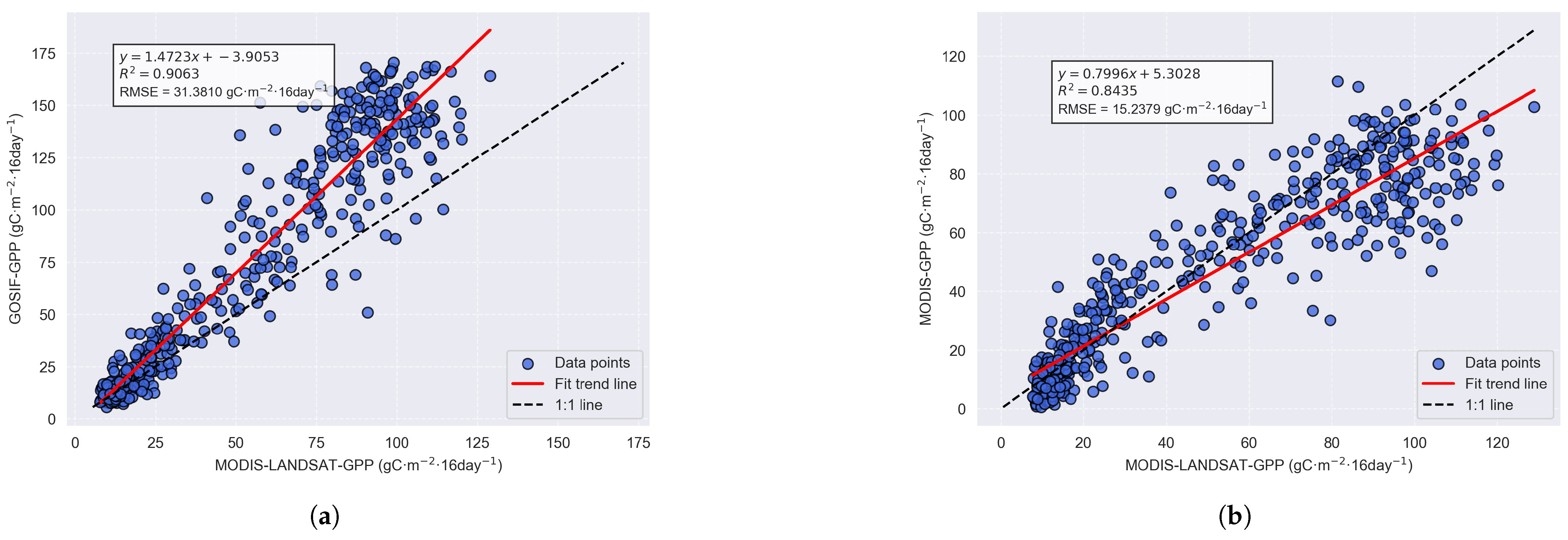
As shown in Figure 2, the between the Landsat GPP estimated by the CASA model and GOSIF GPP reaches 0.9150, while the between the Landsat GPP estimated by the CASA model and MODIS GPP reaches 0.8473. This indicates a high degree of similarity between the GPP estimated by the CASA model and the control groups, demonstrating the reliability and accuracy of the CASA model. The GOSIF GPP shows a higher average GPP, compared to the MODIS-LANDSAT GPP. In contrast, the MODIS GPP shows an underestimation of high values, leading to a lower average GPP relative to the LANDSAT GPP.
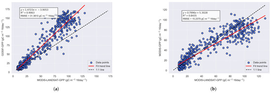
Figure 2.
Fitted trends between the GOSIF GPP, MODIS GPP, and MODIS-LANDSAT GPP estimated by the CASA model. (a) Fitted trend for GOSIF GPP. (b) Fitted trend for MODIS GPP.
3.2. Spatial Distribution Characteristics of GPP
3.2.1. Overall Spatial Distribution
To illustrate the distribution of the annual mean GPP in the study area, yearly GPP data from 2001 to 2020 and the 20-year mean were visualized using ArcGIS (Version 10.8), as shown in Figure 3 (displaying only 2001, 2010, 2020, and the 20-year mean). Overall, the GPP distribution exhibits a west-high, east-low pattern, associated with high forest cover in the west and dominant urban development in the east. By comparing the GPP changes in northwestern Hubei over time, the areas along the Han River and its tributaries show a slightly lower GPP than the surrounding areas, which can be linked to increased development and human activities. Meanwhile, southern northwestern Hubei displays a significant upward GPP trend over time. The Shennongjia Forest District consistently maintains high GPP levels, which can be closely tied to the establishment of forest reserves and the regional ecological restoration policies. In some river areas, GPP values were detected despite being classified as water bodies. This uncertainty may result from mixed pixels or sub-pixel heterogeneity, where water pixels may contain vegetated features such as riparian vegetation, small islands, or shallow water with aquatic plants. Additionally, errors in land cover classification and spatial resolution mismatches may contribute to these values. Therefore, such GPP values are not necessarily erroneous but may reflect actual photosynthetic activity from vegetated elements within nominal water pixels. The reason for low GPP at low elevation may be mostly due to the widespread distribution of cropland and non-vegetated land cover types (Figure 1b), which show much lower GPP than the forests in the high elevation area.
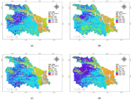
Figure 3.
Spatial distribution of GPP in the study area for different years and the mean over 2001–2020. (a) GPP distribution in the study area for 2001. (b) GPP distribution in the study area for 2010. (c) GPP distribution in the study area for 2020. (d) Mean GPP distribution in the study area (2001–2020).
3.2.2. Distribution of GPP with Elevation
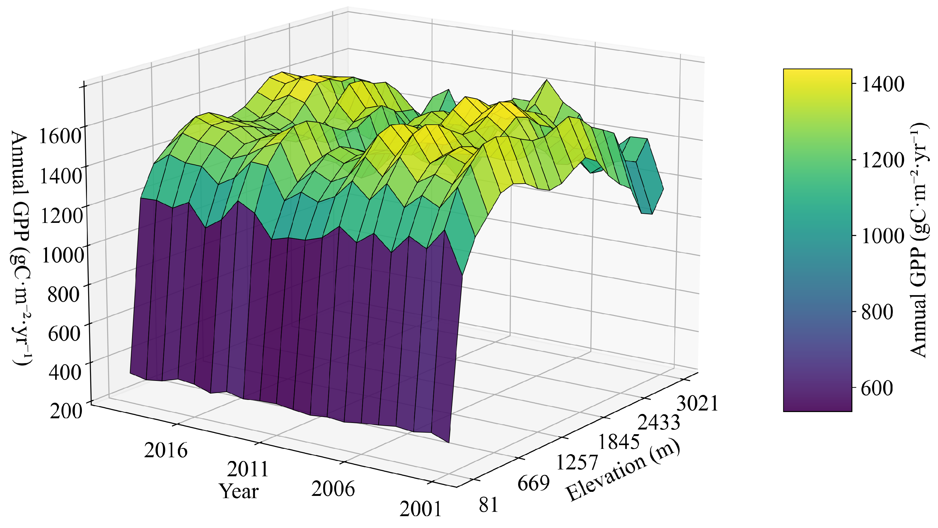
To illustrate the distribution of GPP with elevation, the mean GPP values were calculated and analyzed across different elevation intervals. In addition, a three-dimensional (3-D) plot was employed to visualize the spatial variation in GPP with elevation, as shown in Figure 4. It can be observed that, with increasing elevation, the mean GPP across all the years exhibits an upward trend. This upward trend is particularly pronounced in low-elevation regions, reaching a first peak around 2000 m elevation. After a slight decline, it subsequently reaches a second peak around 3000 m elevation.

Figure 4.
Distribution of GPP with elevation in the study area (the y-axis represents the years, ranging from 2001 to 2020; the x-axis represents the elevation in northwestern Hubei; and the z-axis represents the mean GPP value).
3.3. Temporal Distribution of GPP
3.3.1. Overall Temporal Variation in GPP
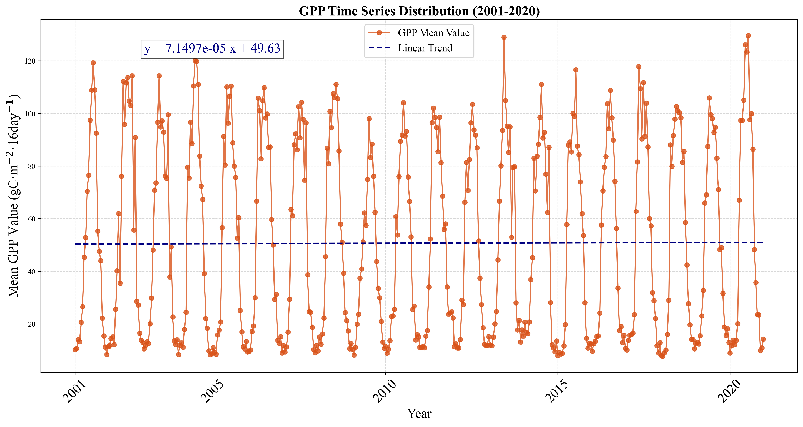
The GPP derived from the Landsat data using the CASA model, with a 16-day temporal resolution, was averaged across the annual and intra-annual time series and visualized as a time series line plot, as shown in Figure 5. Interannually, the annual GPP exhibits a slight upward trend from 2001 to 2020. The GPP shows noticeable interannual fluctuations, particularly in the middle years (i.e., 2009–2012), where the values are relatively stable but do not exhibit significant dips, which is likely due to the balanced climatic conditions during this period. Intra-annually, GPP follows a characteristic “low–high–low” pattern, aligning with the seasonal vegetation growth cycles. At certain intervals, GPP displays a sequence of peaking, declining, and subsequently increasing again, which can be attributed to the interactions between vegetation phenology and climatic drivers, which is a common phenomenon. Peak GPP values typically range from 100 to 140 gC·m−2·16 d−1.
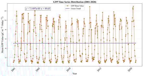
Figure 5.
Temporal distribution of GPP (y-axis: mean GPP value; x-axis: time series at a 16-day resolution).
3.3.2. GPP Variation Trends
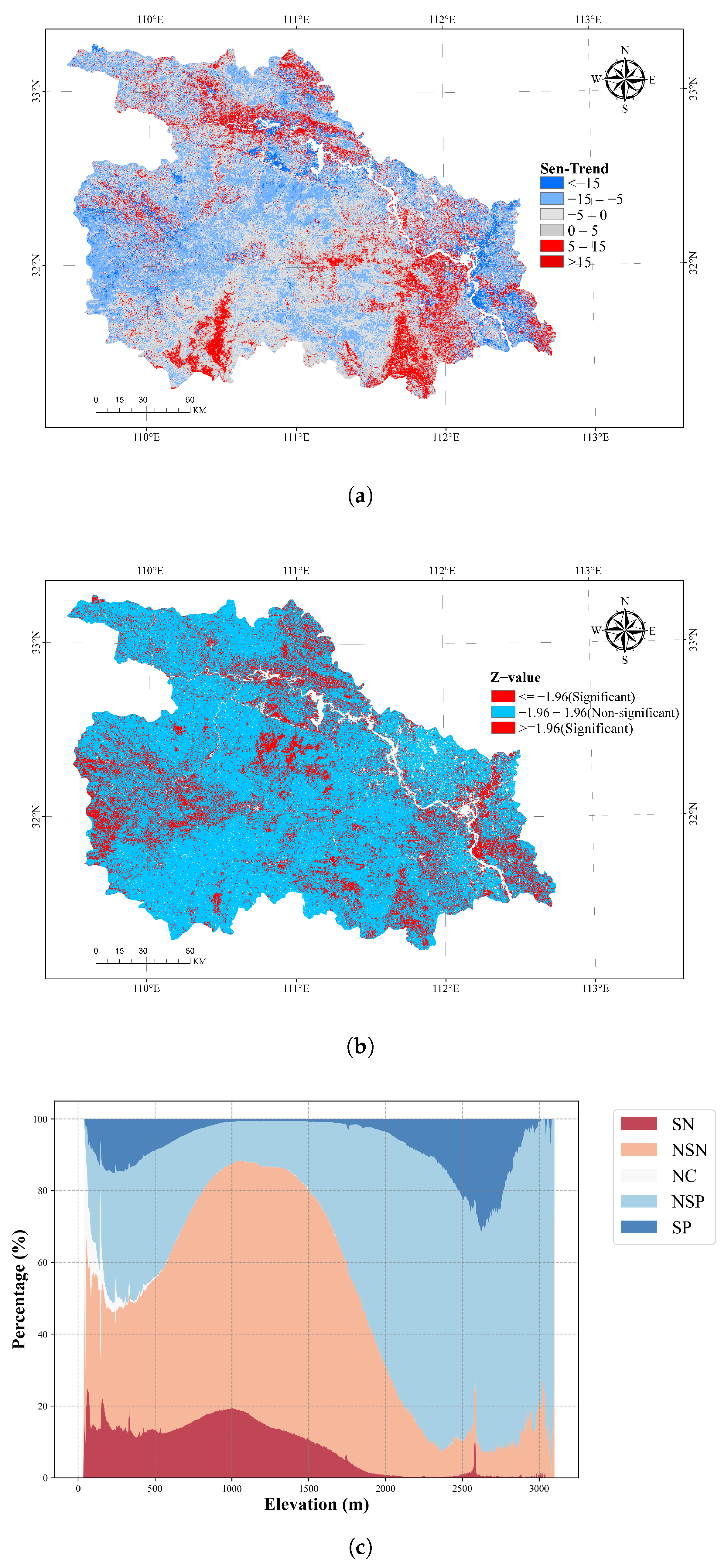
Through the Theil–Sen median slope estimation, the GPP slope of the study area was obtained and visualized using ArcGIS (Version 10.8), as shown in Figure 6a. Firstly, it can be seen that the areas with higher slope values are predominantly distributed at the northern and southern ends, which are regions with greater forest cover density, while the areas with lower slope values are mostly located at the eastern and western ends, corresponding to urban areas directly associated with urban land use and development activities. Overall, there is no significant difference in the area between regions exhibiting an increasing trend and those showing a decreasing trend. However, the area of significant increase surpasses that of significant decrease. Referring to Figure 3d, the regions of significant increase also correspond to areas of higher mean GPP values. Thus, it can be preliminarily concluded that the GPP in the study area exhibits an overall upward trend.

Figure 6.
GPP trend analysis from 2001 to 2020. (a) Theil–Sen median slope of GPP. (b) Z-value of the trend. (c) GPP variation trends (SP: significant positive trend; NSP: non-significant positive trend; NC: no change; NSN: non-significant negative trend; SN: significant negative trend).
The GPP slope was overlaid with the Mann–Kendall trend test for analysis and classified according to the conditions specified in Table 3, yielding the trend classification of the GPP changes in the study area. To more intuitively analyze the distribution of the different trend types, the results were visualized along the elevation distribution, as shown in Figure 6c. Firstly, overall, apart from some unchanged areas in low-elevation regions due to water bodies, the trends of increase and decrease are balanced. However, these trends exhibit opposing patterns with elevation. At elevations of 2000 m and below, a decreasing trend predominates, with significant decreases accounting for approximately 15% and non-significant decreases for about 60%. Above 2000 m, an increasing trend prevails, with significant increases comprising roughly 15% and non-significant increases about 60%. At an elevation of 1000 m, the proportion of significant decreasing trends peaks, indicating substantial impacts from climate change and urban development in this area. At 2500 m, the proportion of significant increasing trends peaks, suggesting notable success in the ecological restoration efforts at this elevation.
3.3.3. Future GPP Trend Prediction
The Hurst exponent of the regional GPP was calculated using Equation (9) and visualized through ArcGIS (Version 10.8), as shown in Figure 7a. Based on the classification conditions in Table 4 combined with Figure 7a, it is evident that most areas with unchanged trends are distributed in the western part, while areas with changing trends are located in the eastern part and some central regions. Referring to Figure 3, it can be observed that regions with changing trends predominantly correspond to areas with low GPP values, whereas regions maintaining their trends are mostly areas with high GPP values.
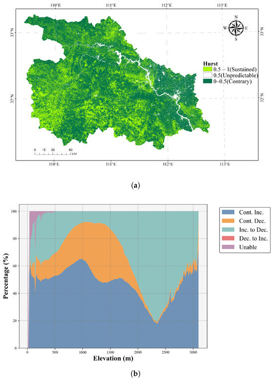
Figure 7.
GPP trend analysis and prediction. (a) GPP Hurst (0–0.5: contrary; 0.5: unpredictable; 0.5–1: sustained). (b) Future GPP trend prediction.
The results of the Hurst exponent were overlaid with the GPP slope results and classified according to the conclusions in Table 4. Due to the limited number of classification categories, an area plot was chosen for visualization along the elevation to provide a more intuitive analysis of the results, as shown in Figure 7b. Firstly, overall, the areas with trends opposite to the original pattern exceed those maintaining the original trend. Among the areas with changing trends, regions shifting from a decreasing to an increasing trend are mostly distributed at elevations of 1500 m and below, while regions shifting from an increasing to a decreasing trend are predominantly found above 1500 m, with both categories having roughly equal proportions. Among the areas maintaining their original trends, those below 2000 m are predominantly characterized by sustained decreases, while those above 2000 m are overwhelmingly characterized by sustained increases, which is closely related to forest cover regions.
3.4. Climate Factor Response Analysis
3.4.1. Comparison of the Climatic Factor Correlations Across Different Scales
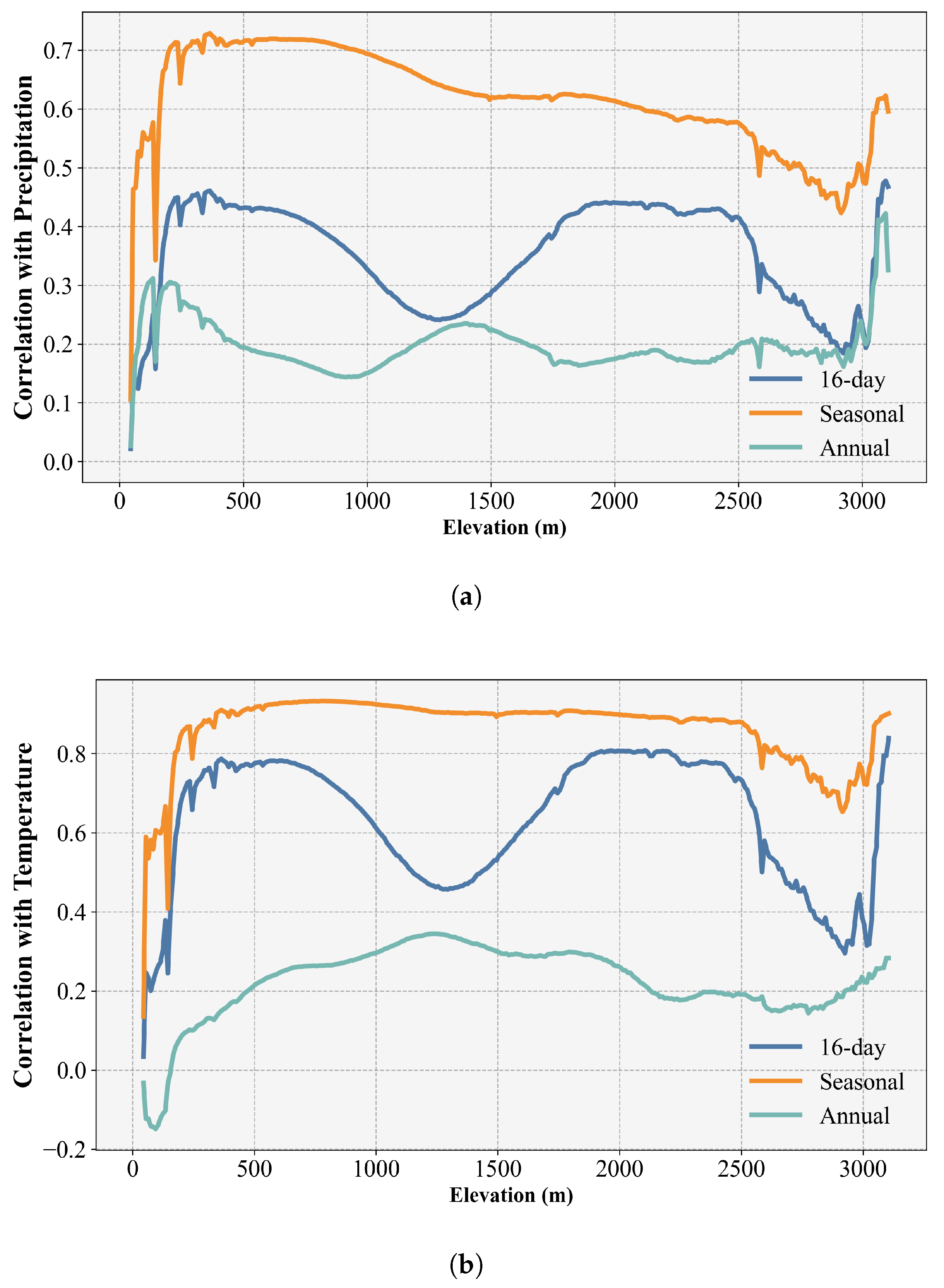
At annual, seasonal, and 16-day scales, the correlations were calculated using the full time series and arranged with elevation for a more intuitive comparison. Figure 8a illustrates the correlation of precipitation with GPP across the different scales with elevation. Firstly, overall, the annual scale exhibits the lowest correlation, the 16-day scale shows a relative increase, and the seasonal scale demonstrates the strongest correlation. This pattern is closely tied to the seasonal variations in precipitation and the seasonal heterogeneity of plant growth. At the annual scale, the GPP variations correlate with the interannual precipitation changes, but these changes are not pronounced year-to-year, resulting in lower correlation. At the 16-day scale, due to the proximity of the time steps, the precipitation differences between adjacent periods are minimal, and vegetation growth typically does not undergo abrupt changes, limiting the increase in correlation. At the seasonal scale, significant seasonal heterogeneity in both precipitation and plant growth leads to the highest correlation between GPP and precipitation. Secondly, analyzing the precipitation correlation changes with elevation reveals a similar overall trend across scales: an initial increase, followed by a decline, and a second peak near the highest elevations. At the annual scale, the precipitation correlation remains relatively stable after reaching the first peak, then rises to a second peak. At the 16-day scale, it drops to a first minimum around 1300 m after the first peak, rises again, reaches a second minimum around 2800 m, and then attains a second peak, reflecting the distribution of vegetation with elevation. At the seasonal scale, the precipitation correlation decreases steadily after peaking, which can be linked to changes in plant species and water demand with increasing elevation, before reaching a second peak at the highest elevation, which is closely related to the vegetation distribution in the Shennongjia region.
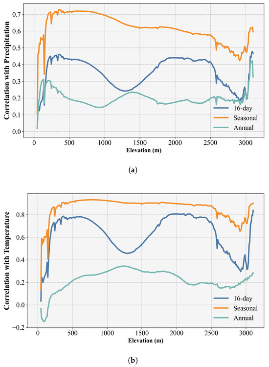
Figure 8.
Correlation between GPP and climatic variables at different temporal scales (including 16-day scale, seasonal scale, and annual scale). (a) Correlation between GPP and precipitation. (b) Correlation between GPP and temperature.
Figure 8b illustrates the correlation of temperature with GPP across different scales with elevation. Firstly, overall, similar to precipitation, the annual scale shows the lowest correlation, the 16-day scale exhibits a relative increase, and the seasonal scale demonstrates the highest correlation. The underlying reasons are largely consistent with those for precipitation, i.e., closely tied to seasonal temperature variations and the seasonal heterogeneity of plant growth. Secondly, analyzing the temperature correlation changes with elevation reveals some differences in trends across scales. At the annual scale, the temperature correlation slightly decreases initially, then rises steadily with elevation, stabilizing around 0.2 with an overall upward trend. At the 16-day scale, it increases with elevation, drops to a first minimum around 1300 m, rises again, reaches a second minimum around 2800 m, and then attains a second peak, mirroring the precipitation correlation pattern at this scale, and is also related to the vegetation distribution with elevation. At the seasonal scale, the temperature correlation increases with elevation, then stabilizes with no significant variation with elevation, slightly decreases around 2800 m, and subsequently rises, which can be closely linked to the vegetation distribution in the Shennongjia region.
3.4.2. Interannual Variations in Climatic Factor Correlations
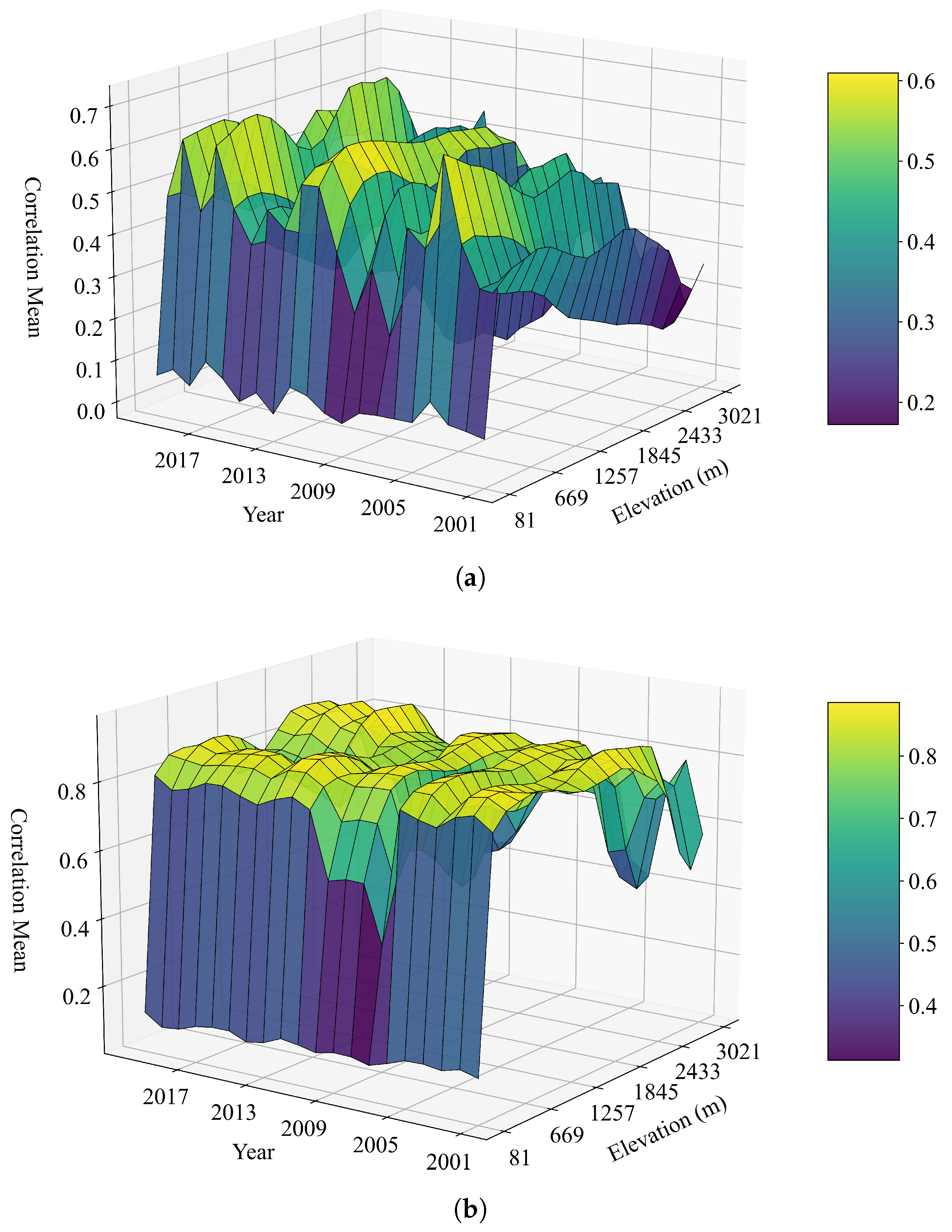
Using the 16-day scale GPP data and climatic factor data, correlation calculations were performed for each year from 2001 to 2020. These correlations were then arranged along the elevation intervals. To better illustrate the interannual variations, a 3D plot was employed for visualization.
Figure 9a shows the distribution of precipitation correlation with elevation for the years 2001 to 2020. Firstly, from an overall perspective, the trend of precipitation correlation across different years with respect to elevation changes is generally similar: it initially increases with elevation, then experiences a certain degree of decline, and subsequently rises again. This pattern is consistent with the trend of precipitation correlation calculated using the entire 16-day scale dataset, as described above. Secondly, in terms of interannual variation, the precipitation correlation with elevation in most years remains at a relatively high level, particularly after 2009, with only slight differences at peak values. In some years, the correlation is at a lower level, which could be related to the precipitation conditions and plant growth in those years. Between 2001 and 2009, the correlation exhibits greater fluctuations, which could be associated with local ecological management and changes in climatic conditions.
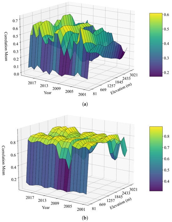
Figure 9.
Interannual variation of the correlation between GPP and climatic variables from 2001 to 2020 in northwestern Hubei (where the x-axis represents the years, the y-axis represents the elevation, and the z-axis represents the mean correlation). (a) Correlation with precipitation. (b) Correlation with temperature.
Figure 9b illustrates the distribution of temperature correlation with elevation for the years 2001 to 2020. Firstly, from an overall perspective, the trend of temperature correlation across different years with respect to elevation changes is generally similar: it increases with elevation, reaches a peak, and then stabilizes gradually. It reaches a first low value around 1300 m, rises again, reaches a second low value around 2800 m, and then attains a second peak. This pattern aligns with the trend of precipitation correlation calculated using the entire 16-day scale dataset, as described above. Secondly, in terms of interannual variation, the correlation in most years remains at a relatively high level, with minimal differences between years, indicating a relatively stable state. The correlation in 2007 is lower than in other years, which is possibly due to the significant temperature deviations in that year compared to others. Overall, the temperature correlation shows little variation between years and consistently maintains a high level.
3.4.3. Intra-Annual Variations in Climate Factor Correlations
Using the 16-day scale GPP data and climatic factor data, correlation calculations were performed for each time point (16-day time scale) within a year, resulting in 23 correlation data points. These results are then arranged along the elevation intervals. To better illustrate the interannual variations, a 3D plot is employed for visualization.
Figure 10a shows the distribution of precipitation correlation variations within a year with elevation. Firstly, from an overall perspective, the trend of precipitation correlation across the different time points within the year is generally similar with respect to elevation changes. Specifically, as elevation increases, the correlation stabilizes at a relatively constant level, with a slight decline around 1300 m. This pattern is consistent with the previously calculated precipitation correlation at a 16-day time scale. Secondly, in terms of the intra-annual variation, the precipitation correlation exhibits a trend of initially increasing and then decreasing over time. The peak occurs between days 193 and 257, corresponding to the summer period.
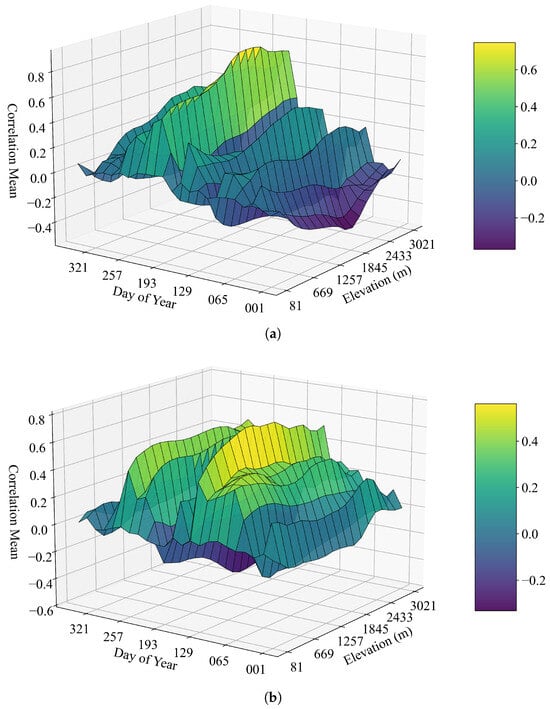
Figure 10.
Intra-annual variation in the correlation between GPP and climatic variables in northwestern Hubei (where the y-axis represents the days, ranging from 1 to 353 (16-day resolution); the x-axis represents the elevation; and the z-axis represents the mean correlation). (a) Correlation with precipitation. (b) Correlation with temperature.
Figure 10b illustrates the distribution of temperature correlation variations within a year with elevation. Firstly, from an overall perspective, the trend of temperature correlation across the different time points within the year is generally similar with respect to elevation changes. Specifically, as elevation increases, the correlation remains relatively stable, with a slight decline around 2800 m, followed by a second peak near the maximum elevation. This pattern aligns with the previously calculated temperature correlation at a 16-day time scale. Secondly, in terms of the interannual variation, the temperature correlation exhibits a pattern of rising, falling, rising again, and then falling over time. Peaks occur between days 129 and 193, as well as between days 257 and 321, corresponding to the periods before and after summer.
4. Discussion
4.1. Novelty of the Work
In northwestern Hubei, the mountainous terrain spawned the high forest cover and rich plant species, which makes the region an important carbon sink. However, the fine distribution and variation in the photosynthetic carbon sequestration from regional plants still remain unclear and lack in-depth exploration, mainly due to the complex and high-dynamic topography and environments in the region requiring finer spatial and temporal resolution monitoring. However, conventional methods based on single-satellite data struggle to fulfill the requirements. This study integrates high-temporal-resolution MODIS NDVI data (16-day intervals) with Landsat data with fine spatial resolution to create a 30 m resolution GPP time series in northwestern Hubei, and analyzed the spatiotemporal variation and climatic responses of photosynthetic carbon sequestration in the region. Compared with previous studies in the same region, this research uses finer data and produces clearer results [35,37,48]. This approach overcomes the spatial limitations of MODIS and the issues of hard-to-obtain time series for Landsat due to cloud cover and longer revisiting cycles. Based on previous studies, we modified the light use efficiency parameters in the CASA model and combined the model with multisource fused remote sensing data to obtian high-resolution GPP estimation in this heterogeneous landscape. By leveraging more detailed spatial data, this research enhances vegetation productivity estimation accuracy and its spatial variation representation, as well as gained insights into climate–vegetation interactions across elevations. Benefiting from the fine spatial resolution, we analyzed the GPP distribution gradients and the variation trends along with elevation, which would greatly impact the temperature and other environmental conditions. Furthermore, we also further explored the climatic controls across different altitudinal gradients at different time scales, as well as their intra-annual and inter-annual variations. Some conclusions were obtained by further considering fine-scale ecological variations, which can provide insights into small-scale mountainous ecological variations and support regional ecological conservation and land management.
4.2. Analysis of Results
In this study, we utilized a multi-source remote sensing data fusion approach, GPP time series at a 16-day temporal resolution, and 30 m spatial resolution in northwestern Hubei from 2001 to 2020, obtained using the revised LUE model. Cross-validation with GOSIF GPP and MODIS GPP products achieved correlation coefficients of R2 = 0.9150 and 0.8473, respectively, confirming the accuracy and reliability of the estimates. However, the RMSE was relatively high, especially for the GOSIF product, which is also widely indicated by many previous studies. This phenomenon can also be mainly attributed to the coarse spatial resolution of the product, as well as the machine learning-based SIF reconstruction and the linear conversion relationship from SIF to GPP [17,49]. To the contrary, many studies have indicated that MODIS data tend to underestimate GPP due to the applied big-leaf model ignoring the contribution of shaded leaves, especially in regions with high GPP [50].
This dataset supported the analysis of regional GPP variations, covering temporal changes, spatial distribution along elevation intervals, and future predictions using the Hurst exponent and Theil–Sen median slope methods. The results of the median slope analysis indicate that high-elevation areas with high GPP values generally exhibit an upward trend, while the plain regions with lower GPP values tend to show a downward trend. This pattern aligns with the fact that high-GPP areas are often located in ecological conservation zones with forest cover in high mountains, where government policies and restoration efforts have been implemented to protect the environment. In contrast, the low-GPP areas covered by cropland in plains are primarily urbanized or developed regions, where increased human activities and land use have contributed to a decline in vegetation productivity.
Subsequently, the relationship between GPP and climatic factors are analyzed to understand the mechanism of GPP distribution and variation, through the computation of Pearson’s correlation coefficients across multiple scales and elevation gradients. The results show that the GPP–climate correlations in northwestern Hubei exhibit notable seasonal heterogeneity, with the seasonal scale displaying stronger relationships than the 16-day or annual scales. This variability can be tied to the elevation-driven climate gradients, such as changes in temperature and precipitation, and the vertical zonation of vegetation, particularly the diverse forest ecosystems in the Shennongjia Forest District. Based on the study of intra-annual correlations, it can be inferred that higher summer temperatures enhance plant photosynthesis intensity, thereby increasing water demand and resulting in a higher correlation with precipitation. Conversely, during the winter months, low-precipitation correlation values are observed as most plants wither, shed leaves, or enter dormancy, exhibiting weak photosynthesis and consequently lower water demand. This leads to a reduced correlation with precipitation, reflecting the strong seasonal differentiation of precipitation correlation. Similarly, as temperatures rise, the temperature correlation with GPP increases. However, during the summer, temperatures may exceed the optimal range for photosynthesis, causing a decline in the temperature correlation. As summer ends and temperatures decrease to more suitable levels for photosynthesis, the temperature correlation rises again. In winter, as temperatures drop sharply, limiting plant photosynthesis, the temperature correlation decreases to a lower level. This highlights the strong seasonal differentiation of the temperature correlation as well.
4.3. Shortcomings of the Work
Although this study has yielded several insights into the spatiotemporal dynamics of GPP in northwestern Hubei, there are still many issue that need further enhancement. In terms of data sources, the current analysis relied primarily on MODIS and Landsat datasets to achieve a balance between temporal frequency and spatial resolution. Integrating additional satellite observations, such as those from the Sentinel constellation, which offer higher spatial resolution (up to 10 m) and improved temporal revisit frequency, could further enhance the precision of NDVI and GPP estimates. During the multi-source remote sensing data fusion process, incorporating sensors with complementary spectral characteristics or cloud-penetrating capabilities may improve the accuracy and temporal continuity of the fused products. Nonetheless, it is important to note that multi-source fusion is inherently subject to certain uncertainties and potential instabilities, arising from sensor discrepancies, differences in radiometric calibration, and preprocessing protocols. These factors may introduce noise or artifacts, particularly in heterogeneous landscapes such as mountainous regions. Expanding and refining the range of input datasets may help to mitigate these challenges by improving robustness and ensuring more consistent spatiotemporal coverage across the complex topography of northwestern Hubei [51].
Regarding the model, in this study, we utilized a big-leaf CASA LUE model, which offers computational simplicity but assumes uniform canopy properties. However, model parameters play a crucial role in accurately estimating GPP. Due to the lack of observational data, parameter calibration in this study remains limited [52]. Future work may require the acquisition of more accurate and site-specific parameters to improve model reliability. Additionally, more advanced modeling approaches could be explored, such as two-leaf LUE models that differentiate between sunlit and shaded leaves, or process-based models that incorporate detailed physiological and environmental interactions. These models could enhance the precision of GPP estimation, particularly in heterogeneous landscapes such as northwestern Hubei, where vegetation types vary significantly with elevation.
Finally, in terms of the analysis, in this study, we focused on Pearson correlation coefficients to examine the GPP–climate relationships. One limitation of this approach is that, due to resampling, multiple pixels may share identical climate variable values, which can reduce the credibility of the correlation results. This issue highlights a shortcoming of the current study and should be addressed in future research to ensure more robust conclusions. Similarly, while the Theil–Sen median slope estimator and Mann–Kendall test are widely used for detecting monotonic trends due to their robustness against outliers and non-normal data, they also present limitations. Specifically, these methods are primarily designed to detect linear or monotonic trends and may fail to capture nonlinear or seasonal patterns in GPP time series. Moreover, the Mann–Kendall test can be sensitive to heteroscedasticity and autocorrelation, potentially affecting the reliability of significance testing. In addition, the use of the Hurst exponent to analyze the persistence or long-term memory of GPP time series is also limited, as it cannot fully capture short-term fluctuations or nonlinear dependencies. To overcome these limitations, future research could incorporate nonlinear trend detection techniques, as well as methods that explicitly account for temporal autocorrelation. In addition, methods such as causal inference or structural equation modeling could be employed to better distinguish correlation from causation. Incorporating other influential factors—such as soil moisture or land use changes, which are relevant to the region’s ecological context—could further broaden the scope of the analysis. These improvements would help capture a wider range of drivers affecting GPP dynamics.
Future research should also explore the applicability of the models across different regions with varying ecological and climatic conditions. The big-leaf CASA LUE model, while efficient, may face limitations in heterogeneous landscapes. Testing its performance in diverse regions and extending advanced models, like two-leaf LUE or process-based models, will help assess their robustness and guide more region-specific GPP estimation approaches.
5. Conclusions
In this study, we elucidated the ecological dynamics of photosynthetic carbon sequestration in northwestern Hubei from 2001 to 2020, highlighting distinct patterns across temporal and spatial dimensions. The interannual GPP exhibited relative stability, suggesting sustained ecosystem output, while the intra-annual fluctuations mirrored the seasonal vegetation cycles, with peak productivity during the growing months. Spatially, the Theil–Sen median slope analysis revealed rising GPP in forested high-value areas, such as the Shennongjia Forest District, contrasted by declines in urbanized low-value zones, reflecting the impact of land cover differences. The Hurst exponent suggested that forested areas may continue to see GPP increases, providing a perspective on the long-term ecological trends.
The climatic drivers shaped the GPP responses, with notable variations across seasons and elevations from 42 m to 3103 m. The seasonal-scale analyses showed stronger GPP correlations with precipitation and temperature, compared to the 16-day or annual scales, indicating significant seasonal heterogeneity. Temperature influences generally intensified with elevation before stabilizing, while precipitation effects followed a pattern of increase, mid-elevation decrease, and subsequent recovery, aligning with moisture availability. These patterns, driven by the climatic variations and vegetation zonation, particularly the rich forest ecosystems of Shennongjia, underscore the complex environmental interactions in mountainous regions. The findings suggest that seasonal and altitudinal factors are critical to GPP dynamics, offering insights for ecological conservation and carbon management in northwestern Hubei. By highlighting these ecological responses, this study provides a reference for addressing climate-driven changes in similar terrain, supporting strategies for sustainable ecosystem management.
Author Contributions
Conceptualization, D.B. and X.G.; methodology, D.B. and Y.W.; software, D.B. and Y.M.; validation, D.B.; formal analysis, D.B.; resources, H.L.; data curation, D.B. and Y.W.; writing—original draft, D.B.; writing—review and editing, X.G.; visualization, D.B.; supervision, X.G.; funding acquisition, X.G. All authors have read and agreed to the published version of the manuscript.
Funding
This research was supported by the National Natural Science Foundation of China (U23A2021, 42371364).
Data Availability Statement
The data used in the paper are available on request from the corresponding author.
Conflicts of Interest
The authors declare no conflicts of interest.
References
- Ahlström, A.; Xia, J.; Arneth, A.; Luo, Y.; Smith, B. Importance of vegetation dynamics for future terrestrial carbon cycling. Environ. Res. Lett. 2015, 10, 054019. [Google Scholar] [CrossRef]
- Simonich, S.L.; Hites, R.A. Importance of vegetation in removing polycyclic aromatic hydrocarbons from the atmosphere. Nature 1994, 370, 49–51. [Google Scholar] [CrossRef]
- Scheffer, M.; Holmgren, M.; Brovkin, V.; Claussen, M. Synergy between small-and large-scale feedbacks of vegetation on the water cycle. Glob. Change Biol. 2005, 11, 1003–1012. [Google Scholar] [CrossRef]
- Ashton-Butt, A.; Aryawan, A.A.; Hood, A.S.; Naim, M.; Purnomo, D.; Suhardi; Wahyuningsih, R.; Willcock, S.; Poppy, G.M.; Caliman, J.P. Understory vegetation in oil palm plantations benefits soil biodiversity and decomposition rates. Front. For. Glob. Change 2018, 1, 10. [Google Scholar] [CrossRef]
- Houghton, R.; Hall, F.; Goetz, S.J. Importance of biomass in the global carbon cycle. J. Geophys. Res. Biogeosci. 2009, 114, G00E03. [Google Scholar] [CrossRef]
- Mitchard, E.T. The tropical forest carbon cycle and climate change. Nature 2018, 559, 527–534. [Google Scholar] [CrossRef]
- Friedlingstein, P. Carbon cycle feedbacks and future climate change. Philos. Trans. R. Soc. A Math. Phys. Eng. Sci. 2015, 373, 20140421. [Google Scholar] [CrossRef]
- Liao, Z.; Zhou, B.; Zhu, J.; Jia, H.; Fei, X. A critical review of methods, principles and progress for estimating the gross primary productivity of terrestrial ecosystems. Front. Environ. Sci. 2023, 11, 1093095. [Google Scholar] [CrossRef]
- Xie, S.; Mo, X.; Hu, S.; Liu, S. Contributions of climate change, elevated atmospheric CO2 and human activities to ET and GPP trends in the Three-North Region of China. Agric. For. Meteorol. 2020, 295, 108183. [Google Scholar] [CrossRef]
- Chen, S.; Zou, J.; Hu, Z.; Lu, Y. Climate and vegetation drivers of terrestrial carbon fluxes: A global data synthesis. Adv. Atmos. Sci. 2019, 36, 679–696. [Google Scholar] [CrossRef]
- Running, S.W.; Zhao, M. Daily GPP and annual NPP (MOD17A2/A3) products NASA Earth Observing System MODIS land algorithm. In MOD17 User’s Guide; MODIS Land Team: Greenbelt, MD, USA, 2015; pp. 1–28. [Google Scholar]
- Sun, Z.; Wang, X.; Zhang, X.; Tani, H.; Guo, E.; Yin, S.; Zhang, T. Evaluating and comparing remote sensing terrestrial GPP models for their response to climate variability and CO2 trends. Sci. Total Environ. 2019, 668, 696–713. [Google Scholar] [CrossRef] [PubMed]
- Wang, K.Q.; Wang, H.S.; Sun, O.J. Application and comparison of remote sensing GPP models with multi-site data in China. Chin. J. Plant Ecol. 2017, 41, 337–347. [Google Scholar] [CrossRef]
- Running, S.W.; Hunt, E.R. Generalization of a forest ecosystem process model for other biomes, BIOME-BGC, and an application for global-scale models. Scaling Physiol. Process. Leaf Globe 1993, 141, 158. [Google Scholar]
- Pei, Y.; Dong, J.; Zhang, Y.; Yuan, W.; Doughty, R.; Yang, J.; Zhou, D.; Zhang, L.; Xiao, X. Evolution of light use efficiency models: Improvement, uncertainties, and implications. Agric. For. Meteorol. 2022, 317, 108905. [Google Scholar] [CrossRef]
- Lees, K.J.; Khomik, M.; Quaife, T.; Clark, J.M.; Hill, T.; Klein, D.; Ritson, J.; Artz, R.R. Assessing the reliability of peatland GPP measurements by remote sensing: From plot to landscape scale. Sci. Total Environ. 2021, 766, 142613. [Google Scholar] [CrossRef]
- Zhang, Y.; Ye, A. Would the obtainable gross primary productivity (GPP) products stand up? A critical assessment of 45 global GPP products. Sci. Total Environ. 2021, 783, 146965. [Google Scholar] [CrossRef]
- Turner, D.P.; Ritts, W.D.; Cohen, W.B.; Gower, S.T.; Zhao, M.; Running, S.W.; Wofsy, S.C.; Urbanski, S.; Dunn, A.L.; Munger, J. Scaling gross primary production (GPP) over boreal and deciduous forest landscapes in support of MODIS GPP product validation. Remote Sens. Environ. 2003, 88, 256–270. [Google Scholar] [CrossRef]
- Li, Z.; Zhang, Q.; Li, J.; Yang, X.; Wu, Y.; Zhang, Z.; Wang, S.; Wang, H.; Zhang, Y. Solar-induced chlorophyll fluorescence and its link to canopy photosynthesis in maize from continuous ground measurements. Remote Sens. Environ. 2020, 236, 111420. [Google Scholar] [CrossRef]
- Xie, X.; Zhao, W.; Yin, G.; Fu, H.; Wang, X. Divergent ecological restoration driven by afforestation along the North and south banks of the Yarlung Zangbo middle reach. Land Degrad. Dev. 2025, 36, 521–532. [Google Scholar] [CrossRef]
- Fang, J.Y.; Ohsawa, M.; Kira, T. Vertical vegetation zones along 30 N latitude in humid East Asia. Vegetatio 1996, 126, 135–149. [Google Scholar] [CrossRef]
- Xie, X.; Tian, J.; Wu, C.; Li, A.; Jin, H.; Bian, J.; Zhang, Z.; Nan, X.; Jin, Y. Long-term topographic effect on remotely sensed vegetation index-based gross primary productivity (GPP) estimation at the watershed scale. Int. J. Appl. Earth Obs. Geoinf. 2022, 108, 102755. [Google Scholar] [CrossRef]
- Xie, X.; Li, A.; Guan, X.; Tan, J.; Jin, H.; Bian, J. A practical topographic correction method for improving Moderate Resolution Imaging Spectroradiometer gross primary productivity estimation over mountainous areas. Int. J. Appl. Earth Obs. Geoinf. 2021, 103, 102522. [Google Scholar] [CrossRef]
- Zhang, Y.; Xu, G.; Li, P.; Li, Z.; Wang, Y.; Wang, B.; Jia, L.; Cheng, Y.; Zhang, J.; Zhuang, S. Vegetation change and its relationship with climate factors and elevation on the Tibetan plateau. Int. J. Environ. Res. Public Health 2019, 16, 4709. [Google Scholar] [CrossRef]
- Zhang, W.; Jin, H.; Li, A.; Shao, H.; Xie, X.; Lei, G.; Nan, X.; Hu, G.; Fan, W. Comprehensive assessment of performances of long time-series LAI, FVC and gpp products over mountainous areas: A case study in the three-River Source region, China. Remote Sens. 2021, 14, 61. [Google Scholar] [CrossRef]
- Zhang, J. Multi-source remote sensing data fusion: Status and trends. Int. J. Image Data Fusion 2010, 1, 5–24. [Google Scholar] [CrossRef]
- He, C.; Gao, B.; Huang, Q.; Ma, Q.; Dou, Y. Environmental degradation in the urban areas of China: Evidence from multi-source remote sensing data. Remote Sens. Environ. 2017, 193, 65–75. [Google Scholar] [CrossRef]
- Petit, C.; Lambin, E.F. Integration of multi-source remote sensing data for land cover change detection. Int. J. Geogr. Inf. Sci. 2001, 15, 785–803. [Google Scholar] [CrossRef]
- Guan, X.; Shen, H.; Wang, Y.; Chu, D.; Li, X.; Yue, L.; Li, W.; Liu, X.; Zhang, L. Fusing MODIS and AVHRR products to generate a global 1-km continuous NDVI time series covering four decades. Big Earth Data 2025, 9, 1–28. [Google Scholar] [CrossRef]
- Luo, M.; Zhou, H.; Liang, Y.; Chen, Z.; Chen, R.; Li, X.; Jakada, H. Horizontal and vertical zoning of carbonate dissolution in China. Geomorphology 2018, 322, 66–75. [Google Scholar] [CrossRef]
- Zhou, S.; Xu, L.; Chen, N. Rice yield prediction in hubei province based on deep learning and the effect of spatial heterogeneity. Remote Sens. 2023, 15, 1361. [Google Scholar] [CrossRef]
- Wang, Y. The regularity of geographical distributions of the vegetation in Hubei Province. J. Wuhan Bot. Res. 1995, 13, 127–136. [Google Scholar]
- Xie, Z.; Shen, G. Outstanding Universal Value and Conservation of Hubei Shennongjia; Springer: Berlin/Heidelberg, Germany, 2021. [Google Scholar]
- Yang, J.; Dong, J.; Xiao, X.; Dai, J.; Wu, C.; Xia, J.; Zhao, G.; Zhao, M.; Li, Z.; Zhang, Y. Divergent shifts in peak photosynthesis timing of temperate and alpine grasslands in China. Remote Sens. Environ. 2019, 233, 111395. [Google Scholar] [CrossRef]
- Chen, Y.; Xie, L.; Liu, X.; Qi, Y.; Ji, X. Identification of high-quality vegetation areas in Hubei Province based on an optimized vegetation health index. Forests 2024, 15, 1576. [Google Scholar] [CrossRef]
- Chen, W.; Huang, C.; Wang, L.; Li, D. Climate extremes and their impacts on interannual vegetation variabilities: A case study in Hubei Province of Central China. Remote Sens. 2018, 10, 477. [Google Scholar] [CrossRef]
- Shi, G.; Ren, F.; Du, Q.; Gao, N. Phytotoponyms, geographical features and vegetation coverage in Western Hubei, China. Entropy 2015, 17, 984–1006. [Google Scholar] [CrossRef]
- Li, X.; Xiao, J. Mapping photosynthesis solely from solar-induced chlorophyll fluorescence: A global, fine-resolution dataset of gross primary production derived from OCO-2. Remote Sens. 2019, 11, 2563. [Google Scholar] [CrossRef]
- Turner, D.P.; Ritts, W.D.; Cohen, W.B.; Gower, S.T.; Running, S.W.; Zhao, M.; Costa, M.H.; Kirschbaum, A.A.; Ham, J.M.; Saleska, S.R. Evaluation of MODIS NPP and GPP products across multiple biomes. Remote Sens. Environ. 2006, 102, 282–292. [Google Scholar] [CrossRef]
- Cheng, Q.; Liu, H.; Shen, H.; Wu, P.; Zhang, L. A spatial and temporal nonlocal filter-based data fusion method. IEEE Trans. Geosci. Remote Sens. 2017, 55, 4476–4488. [Google Scholar] [CrossRef]
- Monteith, J.L. Solar radiation and productivity in tropical ecosystems. J. Appl. Ecol. 1972, 9, 747–766. [Google Scholar] [CrossRef]
- Potter, C.S.; Randerson, J.T.; Field, C.B.; Matson, P.A.; Vitousek, P.M.; Mooney, H.A.; Klooster, S.A. Terrestrial ecosystem production: A process model based on global satellite and surface data. Glob. Biogeochem. Cycles 1993, 7, 811–841. [Google Scholar] [CrossRef]
- Li, J.; Jia, K.; Zhao, L.; Tao, G.; Zhao, W.; Liu, Y.; Yao, Y.; Zhang, X. An Improved Gross Primary Production Model Considering Atmospheric CO2 Fertilization: The Qinghai–Tibet Plateau as a Case Study. Remote Sens. 2024, 16, 1856. [Google Scholar] [CrossRef]
- Ohlson, J.A.; Kim, S. Linear valuation without OLS: The Theil-Sen estimation approach. Rev. Account. Stud. 2015, 20, 395–435. [Google Scholar] [CrossRef]
- Hamed, K.H.; Rao, A.R. A modified Mann-Kendall trend test for autocorrelated data. J. Hydrol. 1998, 204, 182–196. [Google Scholar] [CrossRef]
- Carbone, A.; Castelli, G.; Stanley, H.E. Time-dependent Hurst exponent in financial time series. Phys. A Stat. Mech. Its Appl. 2004, 344, 267–271. [Google Scholar] [CrossRef]
- Cohen, I.; Huang, Y.; Chen, J.; Benesty, J.; Benesty, J.; Chen, J.; Huang, Y.; Cohen, I. Pearson correlation coefficient. In Noise Reduction in Speech Processing; Springer: Berlin/Heidelberg, Germany, 2009; pp. 1–4. [Google Scholar]
- Chen, P.; Pan, H.; Xu, Y.; He, W.; Yao, H. Spatial-Temporal Evolution Characteristics and Driving Force Analysis of NDVI in Hubei Province, China, from 2000 to 2022. Forests 2024, 15, 719. [Google Scholar] [CrossRef]
- Qiu, R.; Han, G.; Ma, X.; Xu, H.; Shi, T.; Zhang, M. A Comparison of OCO-2 SIF, MODIS GPP, and GOSIF Data from Gross Primary Production (GPP) Estimation and Seasonal Cycles in North America. Remote Sens. 2020, 12, 258. [Google Scholar] [CrossRef]
- Huang, X.; Ma, M.; Wang, X.; Tang, X.; Yang, H. The uncertainty analysis of the MODIS GPP product in global maize croplands. Front. Earth Sci. 2018, 12, 739–749. [Google Scholar] [CrossRef]
- Xie, X.; Li, A.; Tian, J.; Wu, C. Analysis of error sources in the multi-scale remote sensing estimation of mountain vegetation gross primary productivity. Natl. Remote Sens. Bull. 2024, 29, 203–218. [Google Scholar] [CrossRef]
- Li, Y.; Xiaobin, G.; Huanfeng, S. Optimal parameter schemes for global and regional gross primary productivity estimation: A comparative analysis. Geo-Spat. Inf. Sci. 2025, 28, 65–84. [Google Scholar] [CrossRef]


Disclaimer/Publisher’s Note: The statements, opinions and data contained in all publications are solely those of the individual author(s) and contributor(s) and not of MDPI and/or the editor(s). MDPI and/or the editor(s) disclaim responsibility for any injury to people or property resulting from any ideas, methods, instructions or products referred to in the content. |
© 2025 by the authors. Licensee MDPI, Basel, Switzerland. This article is an open access article distributed under the terms and conditions of the Creative Commons Attribution (CC BY) license (https://creativecommons.org/licenses/by/4.0/).