Abstract
Understanding the trends and drivers of greenhouse gases (GHGs) is vital to making effective climate mitigation strategies and benefiting human health. In this study, we investigate carbon dioxide (CO2) trends in the top three emitting states in the U.S. (i.e., Texas, California, and Florida) using column-averaged CO2 concentrations (XCO2) from the Greenhouse Gases Observing Satellite (GOSAT) from 2010 to 2022. Annual XCO2 enhancements are derived by removing regional background values (XCO2, enhancement), and their interannual changes (ΔXCO2, enhancement) are analyzed against key influencing factors, including population, gross domestic product (GDP), nonrenewable and renewable energy consumption, and normalized vegetation difference index (NDVI). Overall, interannual changes in socioeconomic factors, particularly GDP and energy consumption, are more strongly correlated with ΔXCO2, enhancement in Florida. In contrast, NDVI and state-specific environmental policies appear to play a more influential role in shaping XCO2 trends in California and Texas. These differences underscore the importance of regionally tailored approaches to emissions monitoring and mitigation. Although renewable energy use is increasing, CO2 trends remain primarily influenced by nonrenewable sources, limiting progress toward atmospheric CO2 reduction.
Keywords:
XCO2; CO2 enhancement; GOSAT; socioeconomic drivers; energy consumption; NDVI; climate change 1. Introduction
Understanding the trends and underlying drivers of greenhouse gases (GHGs) is essential for developing effective climate mitigation strategies. Carbon dioxide (CO2) is the most prevalent GHG and a key contributor to anthropogenic climate change [1,2]. As of 2022, the top three highest CO2-emitting states in the U.S. are Texas, California, and Florida. Texas leads with 663.0 million metric tons of CO2 emissions, followed by California with 326.2 million metric tons and Florida with 231.0 million metric tons [3]. These emissions trends reflect parallel substantial population growth across all three states over the past decade [4]. In 2010, Texas, California, and Florida had populations of 25 million, 37 million, and 18 million, respectively. By 2024, those figures were 31 million, 39 million, and 22 million. Higher populations often translate to greater energy demand, thus potentially amplifying CO2 emissions [5]. These coastal states also host major ports in Houston, Miami, and Los Angeles, contributing heavily to industrial and transportation-related CO2 emissions [6]. Additionally, their large coastal populations are especially vulnerable to sea-level rise and other climate risks [7], highlighting the urgency of monitoring emissions at local to regional scales.
Although various studies have linked anthropogenic activities to elevated atmospheric CO2, fewer have examined how specific socioeconomic and environmental factors, such as energy mix or vegetation cover, influence CO2 concentrations over time and space. In recent studies, satellite-derived column-averaged CO2 (XCO2) and ground-based measurements have been widely used to identify emission sources and analyze the spatial distribution of CO2. For example, Xu and Xiang (2023) [2] analyzed XCO2 levels over ten U.S. states, correlating them with nitrogen dioxide (NO2) and carbon monoxide (CO) to assess anthropogenic impacts. By examining enhancement ratios of CO/XCO2 and NO2/XCO2, they identified states where fossil fuel combustion was the primary contributor to elevated CO2 levels. Similarly, Sheng et al. (2021) [8] utilized column data from the Orbiting Carbon Observatory-2 (OCO-2) and the Greenhouse Gases Observing Satellite (GOSAT), along with ground-based measurements from the World Data Centre for Greenhouse Gases (WDCGG) and CarbonTracker modeling, to investigate trends in XCO2 over China and the eastern U.S. They reported a rise in average XCO2 from 392 ppm (2009–2014) to 406 ppm (2015–2020), with seasonal wintertime enhancements primarily attributed to urban emissions. While such studies underscore the significant role of anthropogenic activities in shaping XCO2 levels, they did not explicitly examine the distinct contributions of energy sources to atmospheric XCO2 patterns.
Satellite-derived XCO2 data products have become increasingly valuable in characterizing atmospheric CO2 trends, analyzing global CO2 fluxes, and validating emissions inventories [9,10]. These platforms offer broad spatial coverage at fine resolution, enabling the analysis of regional carbon dynamics with unprecedented precision. For example, Zheng et al. (2023) [11] demonstrated strong agreement between OCO-2 and GOSAT measurements and ground-based observations from the Total Carbon Column Observing Network (TCCON) across 20 cities worldwide. Another study utilized XCO2 data from OCO-2, OCO-3, GOSAT, and GOSAT-2 and showed that OCO-2 and GOSAT yielded more precise estimates when validated against TCCON [9], reaffirming their utility in long-term monitoring.
In this study, we use long-term GOSAT Level 2 (L2) XCO2 data from 2010 to 2022, supplemented with OCO-2 L2 data for validation, to analyze XCO2 spatiotemporal trends over Texas, California, and Florida. We examine the role of several key drivers, including population, gross domestic product (GDP), energy consumption, and the normalized difference vegetation index (NDVI), to better understand the dynamics behind observed XCO2 trends. Population growth is linked to an increased energy demand and potential CO2 emissions [5]. GDP serves as an indicator of economic growth and energy consumption [12], and a positive correlation between GDP and CO2 emissions has also been observed [13]. Although energy consumption is a primary driver of CO2 emissions [14,15], the composition of the energy mix plays a critical role in determining emissions intensity, an aspect often overlooked in recent studies. For instance, the study by C. Zhang and Lin (2012) [15] did not distinguish between energy sources, while Wu et al. (2020) [14] excluded renewable energy from their analysis. Therefore, our study separates energy consumption into nonrenewable and renewable categories to investigate the distinct impacts of each on atmospheric CO2 levels. Additionally, including NDVI allows us to capture the role of terrestrial carbon uptake through photosynthesis, which fluctuates seasonally [16,17]. By focusing on three of the highest-emitting and fastest-growing states in the U.S., our findings can offer a blueprint for similar analyses in other regions, helping policymakers tailor carbon management strategies to both human and environmental contexts.
2. Materials and Methods
This study utilizes satellite XCO2 data from GOSAT and OCO-2, data from Texas, California, and Florida on population, GDP, and energy consumption, as well as satellite NDVI data from 2010 to 2022 to investigate and explain the changes in XCO2 over these states. Trend analyses of XCO2 and the influencing factors as well as their correlations are performed. We acknowledge that correlation does not imply causation. However, analyzing correlations between CO2 and its potential driving factors can still provide valuable insights into possible associations and underlying patterns. In addition, we conduct multiple linear regression analyses to account for the combined effects of several variables. Nevertheless, given the long atmospheric lifetime of CO2 and the lag between emissions and observed concentration changes, interpreting these regression results is challenging. Therefore, in this study, we focus on reporting correlations with individual factors to highlight the most apparent relationships.
2.1. Study Area
The states chosen for this study are Texas, California, and Florida based on their high annual CO2 emissions as well as their large populations, GDP, and energy consumption.
2.1.1. Texas
Texas is the second largest state in area, behind Alaska, in the U.S. As of 2024, Texas has a population of 31.3 million people, making it the second most populous state [4]. Texas is home to three of the ten most populous cities in the U.S., which are Houston (4th), San Antonio (7th), and Dallas (9th) [18]. It also ranks second in GDP in the U.S., reaching $2.7 trillion in 2024 [19]. Despite being second in size and population, Texas leads in total CO2 emissions, according to the United States Energy Information Administration (U.S. EIA). In 2022, the state emitted 663.0 million metric tons of CO2, which is nearly double that of California, the second-largest emitter [3]. Given Texas’s significant contributions to emissions, understanding the sources and changes in CO2 is vital for shaping effective climate policies and adaptation strategies.
2.1.2. California
California, the third-largest U.S. state by area and the most populous, with 39.4 million residents in 2024 [4], also has the nation’s largest GDP at $4.1 trillion [19]. As the second-highest CO2 emitter, releasing 362.2 million metric tons in 2022 [20], California remains a leader in renewable energy adoption. In 2022, renewables accounted for 49% of the state’s energy mix, followed by natural gas at 42%, with the remaining 9% from other sources. These efforts underscore California’s commitment to addressing climate change through sustainable energy solutions.
2.1.3. Florida
Compared to Texas and California, Florida is smaller in area and population. It is the 26th largest state in the U.S., and has a population of 23.0 million in 2024 [4,21] and the fourth-largest GDP at $1.7 trillion [19,22]. As a major emitter of CO2, with 231.0 million metric tons released in 2022, reducing emissions will be crucial for Florida amid ongoing climate change.
2.2. Satellite Data
2.2.1. XCO2 Data from GOSAT and OCO-2
XCO2 data from the Greenhouse Gases Observing Satellite (GOSAT) and the Orbiting Carbon Observatory-2 (OCO-2) are analyzed, with GOSAT primarily used for trend analysis due to its longer data record, while OCO-2 serves as validation. By integrating both datasets, this study provides a more robust assessment of CO2 changes over Texas, California, and Florida. For each state, L2 XCO2 data are extracted within defined spatial boundaries: Texas (25°N–37°N, 107°W–93°W), California (32°N–43°N, 125°W–113°W), and Florida (24°N–32°N, 88°W–79°W) (Figure 1).
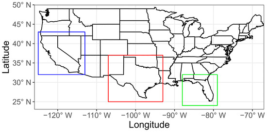
Figure 1.
A map of the United States showing the boundary boxes for Texas (red), California (blue), and Florida (green). For clarity, the colors representing each state remain consistent throughout the manuscript.
The GOSAT mission was launched on January 23, 2009, and became fully operational by 19 April 2009. It is equipped with a Thermal and Near-infrared Sensor for Carbon Observation (TANSO)—featuring a Fourier-Transform Spectrometer (FTS) and a Short-Wave InfraRed (SWIR) detector that measures CO2 in the 1.56–2.08 μm wavelength range of the spectrum. We use the L2 Version 3.05 bias-corrected dataset from Japan’s National Institute for Environmental Studies (NIES), which provides daily measurements at a spatial resolution of 10.5 km × 10.5 km. The dataset was corrected using observations from the Total Carbon Observing Network (TCCON) [23]. We use GOSAT data spanning from January 2010 to December 2022, obtained from the GOSAT Data Archive Service (GDAS) (https://data2.gosat.nies.go.jp/GosatDataArchiveService; last access: 13 March 2025).
The OCO-2 satellite was launched on 2 July 2014, and measures atmospheric CO2 in the near-infrared bands at 1.61 μm and 2.06 μm. It collects eight soundings every 0.333 s across a 0.8-degree swath, enabling high-precision global and regional CO2 monitoring. This study uses OCO-2 L2 Version 11.1r data, which have a spatial resolution of approximately 2.25 km × 1.29 km and a 16-day revisit cycle, covering the period from January 2015 to December 2022. The dataset is available through NASA’s Goddard Earth Science Data Information and Services Center (https://disc.gsfc.nasa.gov; last access: 10 June 2024).
Monthly average XCO2 concentrations from both GOSAT and OCO-2 show consistent, statistically significant increasing trends across Texas, California, and Florida over the past decade (Figure 2a). GOSAT data indicates an XCO2 growth rate of 6.5 ppb/month in Texas and Florida, and 6.4 ppb/month in California. The bias-corrected GOSAT dataset agrees well with OCO-2 observations, supporting the reliability of GOSAT XCO2 measurements. Strong correlations between GOSAT and OCO-2 are observed, with r-values of 0.987 (Texas), 0.991 (California), and 0.979 (Florida), confirming the consistency of the datasets. Figure 2b shows the changes in emissions for the three states as a reference.
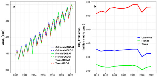
Figure 2.
Temporal variations in (a) the monthly average XCO2 concentrations over California, Florida, and Texas as measured by OCO-2 (2015-2022) and GOSAT (2010–2022), and (b) the annual CO2 emissions for each state as reported by the U.S. EIA.
The differences in XCO2 variations between OCO-2 and GOSAT primarily reflect their distinct spatial sampling strategies. For example, in 2018, OCO-2 provided significantly denser coverage, with 1,032,548 XCO2 retrievals across the three states, compared to just 3067 data points from GOSAT. This lower sampling density in GOSAT may contribute to greater variability, particularly in Florida (197 data points) compared to Texas (1171) and California (1699) [9]. Nonetheless, GOSAT’s long-term record remains valuable for detecting underlying trends by smoothing out short-term variability, thereby supporting investigations into the drivers of XCO2 changes.
2.2.2. Background Calculation and Data Processing
Determining the background concentration of XCO2 is essential for accurately isolating anthropogenic contributions to atmospheric CO2 [24]. As the population, GDP, and energy consumption datasets for each state are all in an annual data format, we calculate the yearly averages of XCO2 as well as the yearly averages of the background concentrations. We extract L2 XCO2 data from GOSAT within spatial boundaries for each state, as defined in Section 2.2.1, and calculate annual XCO2 averages to assess long-term trends. Background XCO2 concentrations are determined by the 5th percentile of observations for each state and year, representing levels minimally influenced by local anthropogenic emissions [2].
Background concentrations of XCO2 (denoted as ) are subtracted from yearly averages (denoted as ) as in Equation (1) to generate the absolute enhancements of XCO2 (denoted as ).
Changes in XCO2 enhancement from year to year (denoted as ) are then calculated using Equation (2) to better correlate CO2 to the inter-annual changes of the influencing factors. We also calculate the relative percent changes of (denoted as %) using Equation (3).
2.3. Data of the Influencing Factors
The influencing factors used for this study are the state’s population, GDP, energy consumption, and NDVI. Interannual differences and relative percent changes in these factors are calculated to assess their influences on CO2 concentrations. In our analysis, each annual dataset comprises 13 samples, while each interannual dataset includes 12 samples.
2.3.1. Population and GDP
Population growth, experienced by each state over the past decade, can have a significant impact on CO2 levels in the atmosphere [25]. Yearly average population data for each state is obtained from the U.S. Census Bureau, covering the period from 2010 to 2022 (https://data.census.gov/; last accessed: 11 March 2025).
Similarly, an increasing GDP indicates economic growth, which could lead to higher energy consumption and enhanced CO2 emissions [13,26]. Yearly average GDP data, beginning in 2010 and ending in 2020, is obtained from the U.S. Bureau of Economic Analysis (https://www.bea.gov/data/gdp; last accessed: 12 March 2025). In this study, we use GDP values measured in chained 2012 dollars to account for inflation.
2.3.2. Renewable and Nonrenewable Energy
Each state’s energy consumption is categorized into nonrenewable and renewable energy sources. Renewable energy includes solar, wind (not used in Florida), hydroelectricity, and biomass waste, the key renewable types considered in this study. Nonrenewable energy encompasses coal, natural gas, petroleum, and nuclear power [20]. Energy consumption data from 2010 to 2022 for both categories for each state are obtained from the U.S. Energy Information Administration (U.S. EIA), with associated CO2 emissions and consumption trends provided by the State Energy Data System (SEDS) (https://www.eia.gov; last accessed: 12 March 2025).
2.3.3. NDVI
The NDVI, often referred to as the “greenness factor”, is a biological proxy for vegetation-driven CO2 uptake across each state. Seasonal changes in atmospheric CO2 are closely linked to photosynthetic activity, which is influenced by vegetation cover [27]. In winter, CO2 levels are typically higher due to minimal uptake by the biosphere, especially in areas dominated by deciduous trees. As spring arrives and vegetation grows, atmospheric CO2 is taken up by increased biospheric activity, continuing into the summer months with increased photosynthesis. In autumn, as trees shed their leaves, CO2 increases again due to weakened photosynthetic activity.
We use NDVI data from the Moderate Resolution Imaging Spectrometer (MODIS) aboard NASA’s Terra satellite, which captures measurements at a given location every 16 days at a 500 m resolution [28]. Monthly NDVI data from January 2010 to January 2023 are used to compute annual averages for 2010 to 2022. This dataset is obtained from the United States Geological Survey’s Land Processes Distributed Active Archive Center (USGS LP DAAC) (https://lpdaac.usgs.gov/products/mod13a1v061/; last accessed: 11 March 2025). Interannual NDVI changes are calculated for each state to assess vegetation trends and their relationship to atmospheric CO2 variability.
3. Results
3.1. Changes in XCO2
We begin by analyzing interannual changes in XCO2 for each state using GOSAT data from 2010 to 2022. In Texas, the annual mean XCO2 increased by approximately 7.29%, while the 5th percentile background concentration increased by about 4.58%, with an average standard deviation of 2.43 ppb (Figure 3a). The XCO2, enhancement ranged from 3.58 ppm in 2012 to 4.94 ppm in 2017 (Figure 3b). The ΔXCO2, enhancement in Texas demonstrated substantial year-to-year variability, especially between 2016 and 2017 (Figure 3c). The %ΔXCO2, enhancement fluctuated between -18.1% and 36.3%, with the largest decrease from 2015 to 2016 and the largest increase from 2016 to 2017. In California, the annual mean XCO2 increased by 7.36%, while background concentrations rose by 7.55% over the same period, with an average standard deviation of 2.63 ppb (Figure 3a). The average enhancement was approximately 4.3 ppm (Figure 3b), with values ranging from 3.64 ppm to 4.79 ppm (Figure 3b). The %ΔXCO2, enhancement demonstrated interannual variation between −15.5% and 23.6% (Figure 3d), reflecting similar trends as observed in Texas. In Florida, both mean and background XCO2 concentrations steadily increased, with a 7.11% rise in annual mean XCO2 and an average standard deviation of 2.54 ppb (Figure 3a). The average enhancement was 4.34 ppm (Figure 3b). Notable changes in ΔXCO2, enhancement that occurred include a large increase of 1.21 ppm from 2012 to 2013, followed by a decrease of 1.66 ppm from 2019 to 2020 (Figure 3c).
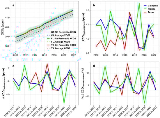
Figure 3.
Temporal variations in (a) annual mean and background XCO2 concentrations, with their standard deviations indicated by shaded areas, (b) mean XCO2, enhancement (Equation (1)), (c) interannual differences in XCO2, enhancement (ΔXCO2, enhancement; Equation (2)), (d) relative percent changes in XCO2, enhancement (%ΔXCO2, enhancement; Equation (3)), as measured by GOSAT over Texas, California, and Florida from 2010 to 2022.
All three states exhibited concurrent increases in XCO2, enhancement during the periods from 2012 to 2013, 2016 to 2017, and 2020 to 2021. These coordinated increases may reflect broader regional or national-scale influences, such as economic expansion or heightened fossil fuel consumption during those years. The increase from 2012 to 2013 could be attributed to an increase in energy demand due to the colder weather the nation experienced during this time, thus releasing more CO2 into the atmosphere [29]. The sharp rise from 2016 to 2017 coincided with a period of significant industrial activity, particularly in Texas, which experienced a surge in energy production and consumption [30]. The increase from 2020 to 2021 followed the initial economic downturn during the COVID-19 pandemic, reflecting a post-pandemic economic rebound with an increase in CO2 due to increased energy consumption [31].
In contrast, decreases in XCO2, enhancement are observed across all states during 2011 to 2012, 2013 to 2014, and 2017 to 2018, potentially indicating reductions in anthropogenic emissions due to factors such as milder winters, policy-driven emissions cuts, or shifts in energy consumption patterns. The decline from 2011 to 2012 may be related to relatively mild winter temperatures across much of the U.S., reducing heating-related emissions [32]. The 2013 to 2014 decrease could be linked to the increased integration of renewable energy sources, especially solar energy use in California with their Renewables Portfolio Standard (RPS), and greater energy efficiency efforts [33]. The drop from 2017 to 2018 aligned with a temporary slowdown in economic growth and a reduced energy demand, and also reflected a shift in energy usage, from coal to natural gas and renewables [34].
The annual CO2 emissions for Texas, California, and Florida generally increased from 2010 to 2022, except from 2019 to 2020 due to the COVID-19 pandemic with stay-at-home orders in place (Figure 2b). It is important to note that changes in CO2 emissions do not result in immediate or proportional changes in atmospheric CO2 concentrations, due to the long atmospheric lifetime and wind-driven transport of CO2. While a fraction of emitted CO2 is removed from the atmosphere within a few years by land and ocean sinks, a significant portion remains in the atmosphere much longer, approximately 25% persists for over 1000 years [35]. Additionally, unlike surface measurements, column-averaged concentrations are more influenced by atmospheric mixing and large-scale transport, making them less sensitive to short-term, localized emissions but well-suited for detecting long-term, large-scale trends, as in this study. Analyzing year-to-year changes in XCO2 alongside potential emission drivers within this timeframe can offer meaningful insights into their role in shaping state-level and decadal CO2 trends.
3.2. Variations of the Influencing Factors
We then examine and compare variations in the selected key influencing factors over the past decade across the three states. This analysis of individual factors establishes the baseline development status of each state, providing context for interpreting CO2 changes in the subsequent correlation analysis.
The populations of Texas, California, and Florida increased each year during the study period (Figure 4a). While the populations steadily increased, the interannual change generally declined from 2010 to 2020 in Texas and California (Figure 4b,c). In contrast, Florida showed increasing interannual population change until 2016, followed by a decline through 2020. From 2020 to 2022, interannual population change increased in both Texas and Florida, while California experienced a notable decline, likely due to population outflow during COVID-19 work-from-home policies and rising living costs [36,37].
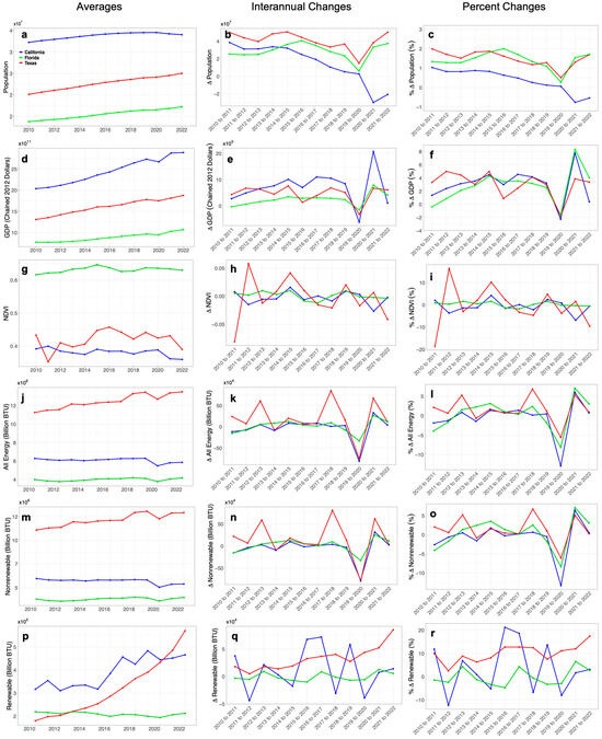
Figure 4.
Temporal variations in (a,d,g,j,m,p) annual averages, (b,e,h,k,n,q) interannual changes (current year–previous year), and (c,f,i,l,o,r) interannual relative percent changes ([current year–previous year]/previous year] × 100) for (a–c) population, (d–f) GDP, (g–i) NDVI, (j–l) total energy consumption, (m–o) nonrenewable energy consumption, and (p–r) renewable energy consumption across Texas, California, and Florida over the period of 2010–2022.
Similar to population, each state’s annual average GDP increased over the 2010–2022 period (Figure 4d,e). From 2010 to 2019, Texas, California, and Florida showed growth rates of about 35.9%, 34.0%, and 24.6%, respectively. All three states experienced a decline in GDP from 2019 to 2020 due to the COVID-19 pandemic, followed by a resumed upward trend thereafter (Figure 4e,f) [38].
NDVI values varied distinctly across the three states (Figure 4g–i). In Texas and California, severe summer droughts often led to declines in NDVI [39] (Figure 4h). For example, in 2011, Texas experienced one of the worst droughts on record, according to the U.S. Drought Monitor (USDM), causing substantial agricultural damage and a significant NDVI drop from 0.43 to 0.35, an approximate 18% decrease (Figure 4i) [40]. Texas showed the greatest NDVI variability over the decade, while Florida maintained the most stable values, averaging approximately 0.63. Texas averaged 0.42, and California, which also experienced notable droughts, particularly between 2012 to 2016, averaged around 0.38 [41].
Total energy consumption, including both nonrenewable and renewable sources, increased from 2010 to 2022 in Texas (Figure 4j). Interannual changes in total energy consumption revealed a sharp decline in 2020 across all three states, likely due to the COVID-19 pandemic (Figure 4k) [42]. From 2019 to 2020, total energy consumption declined by 6.10% in Texas, 12.9% in California, and 8.11% in Florida (Figure 4l). Nonrenewable energy consumption trends mirrored those of total energy use, although at a slightly lower magnitude (Figure 4m–o), as all three states continued to rely heavily on nonrenewable resources. In contrast, renewable energy consumption patterns varied widely (Figure 4p–r). California and Texas quickly expanded their use of renewable resources, while Florida’s adoption progressed more slowly. Texas’s renewable energy use grew from 179,942 billion Btu in 2010 to 570,754 billion Btu in 2022 (Figure 4p). California’s renewable energy consumption increased from 316,810 billion Btu to 466,164 billion Btu over the same period. In contrast, Florida saw a slight decline from 218,948 billion Btu in 2010 to 211,997 billion Btu in 2022. Interannual changes in renewable energy use in Texas remained consistently positive or increased each year, while California and Florida exhibited both positive and negative fluctuations, indicating greater variability in growth patterns (Figure 4q,r).
The analysis of key socioeconomic and environmental indicators—population, GDP, NDVI, and energy consumption—highlights significant differences in the developmental and ecological trajectories of Texas, California, and Florida over the past decade. Texas consistently demonstrated growth across most metrics, particularly in renewable energy expansion. California exhibited slower population growth alongside more pronounced renewable energy use fluctuations, while Florida showed relatively stable vegetation and more modest changes in energy and economic variables.
3.3. Variations in Specific Energy Types
Texas exhibits substantial shifts in both nonrenewable and renewable energy consumption from 2010 to 2022 (Figure 5a and Figure 6a). Nonrenewable energy sources, namely coal, natural gas, nuclear, and petroleum, consistently dominated total energy consumption compared to renewable sources such as wind, solar, hydroelectric (hydro), and biomass waste. Over this period, coal consumption showed a sustained decline, whereas natural gas and petroleum consumption increased (Figure 5a). This trend was also observed nationally, reflecting the lower cost of natural gas and petroleum compared to coal, as well as increasingly stringent regulations on coal-fired power plants [43]. From 2010 to 2022, natural gas and petroleum consumption in Texas increased by 34.9% and 21.9%, respectively, whereas coal consumption declined by 40.5% (Figure 5c). The COVID-19 pandemic in 2020 contributed to a temporary drop in petroleum use due to lockdown measures and reduced mobility. According to Vaz (2022) [44], petroleum consumption decreased by 11.4% across the U.S. due to lockdown restrictions. In Texas, petroleum consumption decreased by 9.74% (Figure 4b,c). After the pandemic, petroleum consumption rebounded, rising by 6.45% by 2022 relative to 2020. In contrast to the other nonrenewable energy sources, nuclear energy consumption remained largely stable over the study period, with only a 0.44% increase, from 432,036 billion Btu in 2010 to 433,919 billion Btu in 2022 (Figure 5a).
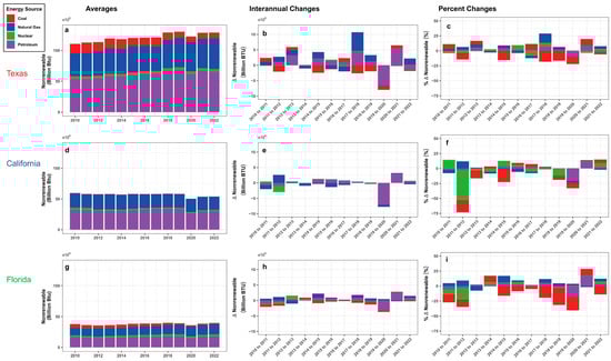
Figure 5.
Temporal variations in nonrenewable energy consumption from 2010 to 2022 are shown for (a–c) Texas, (d–f) California, and (g–i) Florida, including (a,d,g) average annual values, (b,e,h) interannual differences, and (c,f,i) relative percent changes.
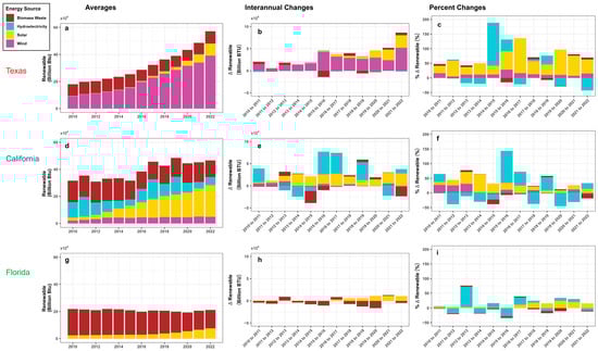
Figure 6.
Temporal variations in renewable energy consumption from 2010 to 2022 are shown for (a–c) Texas, (d–f) California, and (g–i) Florida, including (a,d,g) average annual values, (b,e,h) interannual differences, and (c,f,i) relative percent changes.
Renewable energy consumption has grown substantially in Texas over the past decade, driven primarily by significant increases in wind and solar energy use (Figure 6a). From 2010 to 2022, the consumption of wind and solar energy increased consistently each year (Figure 6b). Over this period, wind energy consumption increased from 89,570 billion Btu to 391,653 billion Btu, a 337.3% increase, while solar energy consumption grew from 630 billion Btu to 87,388 billion Btu, an increase of 13,771.1% (Figure 6b,c). Texas’s expanding population and energy demand, combined with its vast land area, support large-scale renewable energy development, especially wind energy in the Panhandle and western regions [45]. In contrast, energy consumption from biomass waste increased modestly, in comparison to solar and wind energy, by 4.87% over the same period (Figure 6c). Hydroelectricity consumption, however, decreased by 50.8% from 2010 to 2022. This reduction is likely due to both the limited number of hydroelectric power plants in Texas, fewer than 20, and recurrent drought conditions that constrain hydroelectric generation [46,47].
Although California derives a larger share of its energy from renewable sources compared to many other states, petroleum and natural gas remained the dominant energy sources from 2010 to 2022 (Figure 5d). Natural gas consumption steadily decreased by 13.2% from 2012 to 2022 (Figure 5f). In contrast, petroleum consumption increased until 2020, when it dropped sharply due to the COVID-19 pandemic and associated lockdowns [48]. Specifically, petroleum energy consumption decreased from 2,218,732 billion Btu in 2019 to 2,153,254 billion Btu in 2020, a 20.8% decline within one year (Figure 5e). Following the easing of lockdown restrictions, petroleum consumption rebounded by 13.1% in 2022 (Figure 5f). During the 2010–2022 period, coal and nuclear energy consumption in California decreased by 45.3% and 45.5%, respectively (Figure 5f). Coal use in California is minimal, owing to the absence of in-state coal reserves and the presence of only one coal-fired facility [49]. Nuclear energy consumption peaked in 2011 but fell by 49.4% the following year after the permanent shutdown of the San Onofre Nuclear Generation Station, one of the state’s two nuclear power plants [50].
Renewable energy plays a central role in California’s energy strategy. The state has set ambitious targets to meet 100% of retail electricity demand with renewable resources by 2045 [51]. Among the renewable sources, solar and wind energy have shown the most substantial growth. Solar energy consumption increased significantly during the 2010–2022 period, rising from 22,602 billion Btu in 2010 to 232,908 billion Btu in 2022, a 930.5% increase (Figure 6e,f). The growth accelerated after 2014, coinciding with the implementation of the Renewables Portfolio Standard, which required electricity providers to source 33% of their electricity from renewable sources by 2020 [52]. Widespread residential adoption of rooftop solar systems and the commissioning of utility-scale solar power plants further contributed to this expansion. Wind energy consumption also increased substantially over the same period, with a 140.8% rise from 2010 to 2022 (Figure 6f). In contrast, hydroelectric and biomass waste energy consumption declined by 47.2% and 22.8%, respectively. Hydroelectricity generation is highly sensitive to interannual variability in precipitation and snowpack, leading to greater fluctuations [49]. Meanwhile, the steady decline in biomass waste is attributed to limited policy support, competition from more cost-effective renewable resources such as solar and wind, and increasing development costs [53].
Florida exhibited notable changes in both nonrenewable and renewable energy consumption during the 2010–2022 period (Figure 5h and Figure 6h). Nonrenewable sources, particularly petroleum and natural gas, dominated the state’s energy profile, while coal consumption declined steadily, and nuclear energy consumption showed a gradual increase since 2012 (Figure 5g). On average, natural gas and petroleum consumption were approximately 1.4 and 1.7 million billion Btu, respectively, while coal averaged 396,177.3 billion Btu (Figure 5h). Coal consumption decreased by 73.0% throughout this period, while natural gas and petroleum consumption increased by 40.6% and 5.55% (Figure 5i). The decline in coal use is largely attributed to a statewide transition toward natural gas as a cleaner and more cost-effective alternative [54]. Although petroleum consumption increased steadily over much of the period, it declined sharply by 17.7% in 2020, from 1,805,377 billion Btu to 1,485,585 billion Btu, in response to mobility restrictions and reduced economic activity during the COVID-19 pandemic (Figure 5h,i) [42]. Nuclear energy consumption increased consistently, with a notable rise between 2012 and 2013, when Florida’s two nuclear plants, St. Lucie and Turkey Point, completed upgrades that added more than 500 megawatts of capacity to each plant [55].
Florida’s renewable energy profile, comprising solar, hydroelectric, and biomass waste, demonstrated divergent trends between 2010 and 2022 (Figure 6g). Biomass waste consumption steadily declined, while solar energy consumption increased, and hydroelectricity remained relatively stable over the decade (Figure 6g). Solar energy consumption, in particular, began to rise more rapidly in recent years, from 23,969 billion Btu in 2010 to 74,750 billion Btu by 2022, representing a 211.9% increase (Figure 6h). The increase in solar energy consumption is likely due to infrastructure expansion implemented around 2020 [56]. In contrast, hydroelectricity consumption exhibited minimal variation, increased by 30.0% from 2010 to 2022 (Figure 6i). The limited change is consistent with Florida’s constrained hydroelectric capacity, given its flat topography and the presence of only a single operational hydroelectric power plant [57]. Biomass waste consumption decreased by 29.8% during this period, often exhibiting interannual decreases (Figure 6h). This downward trend likely reflects competition from more rapidly expanding sources such as solar, as well as policy and economic barriers to biomass development.
3.4. Correlation Analyses
This section discusses the interannual differences in XCO2, enhancement and related factors. Energy consumption is categorized into total energy use, nonrenewable and renewable sources, and individual energy sources (Figure 7). For correlation analyses using interannual data, the sample size is twelve for each factor and for XCO2, enhancement. Correlation coefficients near +1.0 indicate strong positive relationships, whereas those near −1.0 indicate strong negative relationships. We acknowledge that correlation does not imply causation; however, examining correlations can still provide valuable insights into potential relationships and guide hypotheses for further investigation. References to each factor below also refer to their respective interannual changes.
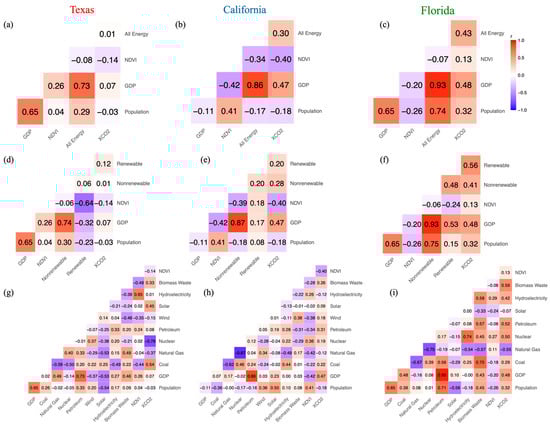
Figure 7.
Correlation matrices of interannual changes in GOSAT-derived XCO2, enhancement, population, GDP, NDVI, and energy-related factors in (a,d,g) Texas, (b,e,h) California, and (c,f,i) Florida from 2010 to 2022. Panels (a–c) show correlations with total energy consumption, (d–f) distinguish between nonrenewable and renewable energy sources, and (g–i) show individual energy sources. A color scale for r values is included in the top panel, on the far right.
In Texas, GOSAT-derived ΔXCO2, enhancement shows no significant correlation with population, GDP, NDVI, or total energy consumption (Figure 7a). In contrast, GDP and total energy consumption are strongly positively correlated (r = 0.78), reflecting nearly identical interannual fluctuations. When energy use is partitioned into nonrenewable and renewable sources (Figure 7d), ΔXCO2, enhancement exhibits no clear relationships with either energy category. However, GDP and nonrenewable energy consumption maintain a strong positive correlation (r = 0.79), consistent with nonrenewables’ dominance of Texas’s overall energy mix (Figure 4j–l and Figure 5a). Breaking energy down by individual source (Figure 6g) reveals that nuclear generation is strongly negatively correlated with ΔXCO2, enhancement (r = −0.78). This is primarily due to pronounced fluctuations in nuclear output from 2015 to 2018 (Figure 5b), which shows an opposite trend to ΔXCO2, enhancement (Figure 3c). Coal consumption, by contrast, exhibits a moderate positive correlation with ΔXCO2, enhancement (r = 0.51), largely driven by parallel declines in both variables from 2017 to 2020 (Figure 5b). Natural gas consumption has a negative correlation with ΔXCO2, enhancement (r = −0.40), likely due to its lower CO2 emissions compared to coal, which emits nearly twice as much CO2 per unit energy [58]. In contrast, biomass waste consumption has a moderate positive correlation with ΔXCO2, enhancement (r = 0.36), as its combustion directly releases CO2, unlike other renewable resources [59].
Among the socioeconomic and biophysical factors, petroleum consumption and GDP have a strong positive correlation (r = 0.77), reflecting Texas’s role as the nation’s leading crude-oil producer. The state’s substantial petroleum industry contributes nearly half of total U.S. crude oil production, linking economic growth closely with petroleum consumption [60]. This relationship is particularly evident after 2015, when interannual changes in petroleum consumption and GDP align closely (Figure 5b and Figure 4f). NDVI and hydroelectricity consumption are strongly positively correlated (r = 0.79), a relationship likely reinforced by the severe 2011 drought. Hydroelectric energy use declined substantially from 2010 to 2011, dropping by 2384 billion Btu (Figure 6b), while NDVI experienced its largest decrease of 0.08 during the same period (Figure 4i).
ΔXCO2, enhancement in California shows stronger correlations with population, GDP, NDVI, or total energy consumption than in Texas (Figure 7b). Several such moderate relationships are notable. ΔXCO2, enhancement is negatively correlated with NDVI (r = −0.35), likely reflecting photosynthetic CO2 uptake, especially during years with significant greening such as 2014–2015 (Figure 4h). A moderate positive correlation is observed with GDP (r = 0.42), potentially linked to California’s post-COVID economic rebound, which outpaced that of Texas and Florida (Figure 4e). Population change shows a weak negative correlation (r = −0.13), consistent with population decline starting around 2016, likely driven by rising living costs (Figure 4b). Petroleum and natural gas are the dominant energy sources in California (Figure 5d). Most energy types, except natural gas and hydroelectricity, show slight positive correlations with ΔXCO2, enhancement (Figure 7e,h), with petroleum showing the strongest, indicating it remains a key driver of CO2 concentrations despite progressive environmental policies.
California’s GDP and total energy consumption exhibit a strong positive correlation (r = 0.85). When energy consumption is broken down into nonrenewable and renewable sources (Figure 7e), a strong positive correlation remains between GDP and nonrenewable energy consumption (r = 0.85), the latter being the dominant energy type in California. Examining individual energy sources, GDP and petroleum consumption are strongly positively correlated (r = 0.84), with their interannual patterns aligning closely beginning in 2013 (Figure 5e), similar to the pattern observed in Texas. Additionally, nuclear and natural gas consumption display a strong negative correlation (r = −0.87), as their interannual changes follow nearly opposite trajectories (Figure 5e), reflecting California’s increasing reliance on natural gas to compensate for the planned phaseout of nuclear power plants [50]. A similar but slightly weaker inverse relationship is seen between natural gas and coal consumption (r = −0.73), likely influenced by California’s Senate Bill 100, which mandates 100% clean electricity retail sales by 2045. Although coal use remains substantially lower than natural gas during the study period, the policy-driven shift away from carbon-intense fuels likely contributes to this inverse trend (Figure 5e) [61].
In contrast to Texas and California, Florida exhibits more distinct correlations between ΔXCO2, enhancement and the influencing factors. Moderate positive correlations are observed with population (r = 0.42), GDP (r = 0.50), and total energy consumption (r = 0.46) (Figure 7c). Consistent with total energy use, renewable (r = 0.52) and nonrenewable energy (r = 0.44) also correlate moderately with ΔXCO2, enhancement (Figure 7f), suggesting that socioeconomic drivers exert a clearer influence on atmospheric CO2 in Florida. Biomass waste energy consumption shows a moderate positive correlation with ΔXCO2, enhancement (r = 0.59), likely driven by direct CO2 emissions from the combustion of biomass waste, a key renewable energy source in Florida, despite its declining interannual consumption (Figure 6g,h).
Beyond CO2, strong internal correlations exist among Florida’s influencing factors. GDP and total energy consumption exhibit a strong positive correlation (r = 0.91), as do GDP and nonrenewable energy use (r = 0.90) and petroleum consumption (r = 0.93), reflecting Florida’s continued reliance on fossil fuels. Population also correlates strongly with both GDP (r = 0.70) and nonrenewable energy consumption (r = 0.80) (Figure 4b,f and Figure 7f). Petroleum consumption closely tracks GDP (r = 0.93) and population (r = 0.79), with all three showing parallel interannual changes (Figure 4b,f and Figure 5h), likely reflecting the influence of Florida’s large transportation sector, driven by tourism [62]. Among energy sources, natural gas use is strongly negatively correlated with coal (r = −0.81), nuclear (r = −0.75), and biomass waste (r = −0.66), and moderately negatively correlated with hydroelectricity (r = −0.45), indicating the increasing reliance on natural gas as Florida’s primary nonrenewable energy source. The weak role of hydroelectricity is expected, as Florida has only one hydroelectric plant, which is insufficient to meet statewide demand [62].
4. Discussion
Texas and California exhibit slightly negative correlations between interannual changes in populations and XCO2, enhancement. While both states experienced steady population growth from 2010 to 2022, their interannual changes began to decline around 2013 (Figure 4a,b). In California, XCO2, enhancement has a stronger correlation with GDP than with population. This aligns with findings by K. Dong et al., (2018) [63], who reported that population changes in North America may be less sensitive to CO2 fluctuations than economic indicators like GDP. Similarly, both states have negative correlations between XCO2, enhancement and NDVI. Compared to Florida, which maintains high NDVI values around 0.63, Texas and California exhibit lower average NDVI (approximately 0.35–0.44) (Figure 4g), largely due to recurring droughts [64]. These environmental constraints likely reduce vegetation productivity, limiting CO2 uptake and contributing to the observed negative correlations.
In contrast, Florida exhibits stronger and more consistent correlations between interannual changes in XCO2, enhancement and both socioeconomic and environmental indicators. The positive correlation with GDP is consistent with the findings of Tzeremes (2018) [65], who noted a unidirectional causal relationship from energy consumption and CO2 emissions to economic growth. This suggests that Florida’s economic development remains closely tied to carbon-intensive sectors, including tourism and transportation. Additionally, petroleum consumption in Florida closely tracks changes in XCO2, enhancement (Figure 6i), emphasizing the role of oil use in driving CO2 emissions in the U.S. [66]. A comparable relationship between coal consumption and CO2 is evident in Texas (Figure 7g).
Differences in state-level policies likely influence the correlation patterns between interannual changes in XCO2, enhancement and energy-related drivers. Texas has implemented regulatory frameworks for geological CO2 storage [67] and has adopted a Priority Action Plan to reduce emissions in key sectors such as industry, transportation, and electric power by 2050 [68]. California has pursued even more aggressive climate action through its 2022 Scoping Plan, aiming for carbon neutrality and zero-emission transportation [69]. In contrast, Florida currently lacks statewide plans targeting GHG emissions or climate change [70], which may contribute to its higher correlation between energy consumption and XCO2, enhancement.
This study has several limitations. Firstly, the analysis is based on annual data from 2010 to 2022, providing only 13 data points. Such a small sample size increases the influence of outliers on the interannual changes in XCO2, enhancement and their correlation with driving factors, particularly for renewable energy. Although numerous studies have reported negative relationships between renewable energy use and CO2 emissions (e.g., Khan et al., 2021; Menyah and Wolde-Rufael, 2010; Ranthilake et al., 2024; Sharif et al., 2019) [71,72,73,74], our analysis finds a positive correlation in Florida between biomass waste consumption and XCO2, enhancement (Figure 6i). This discrepancy may result from Florida’s heavy reliance on biomass as its dominant renewable energy source [57], as well as the limitations of the small dataset. Secondly, due to the long atmospheric lifetime of CO2, the full effects of emission reduction policies may not be observable for many years [35]. Lastly, this study focuses solely on annual averages and does not account for seasonal dynamics in CO2 or NDVI. Prior studies suggest that seasonal variability, particularly summer photosynthesis and winter fossil fuel emissions, may provide deeper insights into the vegetation–CO2 relationship [75], which remains unexplored here due to our focus on annual-scale trends.
5. Conclusions
This study aims to advance understanding of changes in XCO2 over Texas, California, and Florida by analyzing satellite-based measurements from GOSAT, while also examining the influence of population, GDP, energy consumption, and NDVI from 2010 to 2022. Previous research has shown a consistent rise in XCO2 across the U.S. [76,77], and our findings confirm similar trends in all three states. Using GOSAT data, this study highlights the growing XCO2 levels over the past decade and provides one of the first comparative assessments of how key socioeconomic and environmental factors influence XCO2 in these populous states. By analyzing interannual changes, we find nonrenewable energy sources, particularly nuclear (r = −0.78) and coal (r = 0.51), show strong correlations with ΔXCO2, enhancement in Texas. California exhibits weaker but notable associations with GDP (r = 0.42), nonrenewable (r = 0.21), and renewable (r = 0.22) energy consumption. In Florida, petroleum use (r = 0.55), GDP (r = 0.50), population (r = 0.42), and biomass waste (0.59) are key contributors. Overall, interannual changes in socioeconomic factors, particularly GDP and energy consumption, are more strongly correlated with ΔXCO2, enhancement in Florida. In contrast, NDVI and state-specific environmental policies appear to have a stronger correlation with XCO2 trends in California and Texas. These differences underscore the importance of regionally tailored approaches to emissions monitoring and mitigation. Future research at finer spatial and temporal resolutions, including seasonal analyses and model interpretations, will help disentangle the contributions of anthropogenic and biogenic factors to atmospheric CO2 levels. Additionally, advanced methods for detecting anomalies could better isolate localized signals and reduce background biases. Since satellite sampling density varies seasonally, generally higher in summer, future studies should account for these biases and analyze seasonal patterns separately to clarify their impact on observed changes. Although renewable energy use is increasing, CO2 trends remain primarily influenced by nonrenewable sources, limiting progress toward atmospheric CO2 reduction. Understanding the drivers of CO2 changes in each state is essential for informing more effective climate strategies and supporting local and state governments in their efforts to adapt to and mitigate climate change.
Author Contributions
Conceptualization, Y.L.; methodology, S.L. and Y.L.; validation, S.L. and Y.L.; formal analysis, S.L.; investigation, S.L.; resources, Y.L.; data curation, S.L.; writing—original draft preparation, S.L.; writing—review and editing, Y.L., S.L. and M.B.; visualization, S.L.; supervision, Y.L.; project administration, Y.L.; funding acquisition, Y.L. All authors have read and agreed to the published version of the manuscript.
Funding
This research is supported by Dr. Yang Li’s startup funds at Baylor University.
Data Availability Statement
Data are available for use upon request.
Acknowledgments
The authors would like to acknowledge all the parties that provided open-access data. GOSAT data can be downloaded from the GOSAT Data Archive Service (GDAS) (https://data2.gosat.nies.go.jp/GosatDataArchiveService), accessed on 13 March 2025. OCO-2 data can be downloaded from NASA’s Goddard Earth Science Data Information and Services Center (https://disc.gsfc.nasa.gov; last access: 13 March 2025). MODIS data can be downloaded from the United States Geological Survey’s Land Processes Distributed Active Archive Center (USGS LP DAAC) (https://lpdaac.usgs.gov/products/mod13a1v061/), accessed on 11 March 2025. U.S. Census data can be downloaded from the U.S. Census Bureau (https://data.census.gov/). State GDP data can be downloaded from the U.S. Bureau of Economic Analysis (https://www.bea.gov/data/gdp). State energy data can be downloaded from the U.S. Energy Information Administration (U.S. EIA), with associated CO2 emissions and consumption trends provided by the State Energy Data System (SEDS) (https://www.eia.gov).
Conflicts of Interest
The authors declare no conflicts of interest.
Correction Statement
This article has been republished with a minor correction to the readability of figure 3a. This change does not affect the scientific content of the article.
Abbreviations
The following abbreviations are used in this manuscript:
| CO2 | Carbon dioxide |
| XCO2 | Column-averaged carbon dioxide |
| GHG | Greenhouse gases |
| GDP | Gross domestic product |
| NDVI | Normalized difference vegetation index |
References
- Guan, Y.; Keppel-Aleks, G.; Doney, S.C.; Petri, C.; Pollard, D.; Wunch, D.; Hase, F.; Ohyama, H.; Morino, I.; Notholt, J.; et al. Characteristics of Interannual Variability in Space-Based XCO2 Global Observations. Atmospheric Chem. Phys. 2023, 23, 5355–5372. [Google Scholar] [CrossRef]
- Xu, A.; Xiang, C. Assessment of the Emission Characteristics of Major States in the United States Using Satellite Observations of CO2, CO, and NO2. Atmosphere 2023, 15, 11. [Google Scholar] [CrossRef]
- EIA United States—U.S. Energy Information Administration (EIA). Available online: https://www.eia.gov/beta/states/states/tx/rankings (accessed on 13 March 2025).
- U.S. Census Bureau Index of /Programs-Surveys/Popest/Tables/2020–2024/State/Totals. Available online: https://www2.census.gov/programs-surveys/popest/tables/2020-2024/state/totals/ (accessed on 13 March 2025).
- Pata, U.K. Renewable Energy Consumption, Urbanization, Financial Development, Income and CO2 Emissions in Turkey: Testing EKC Hypothesis with Structural Breaks. J. Clean. Prod. 2018, 187, 770–779. [Google Scholar] [CrossRef]
- Ducruet, C.; Polo Martin, B.; Sene, M.A.; Lo Prete, M.; Sun, L.; Itoh, H.; Pigné, Y. Ports and Their Influence on Local Air Pollution and Public Health: A Global Analysis. Sci. Total Environ. 2024, 915, 170099. [Google Scholar] [CrossRef]
- Hauer, M.E.; Evans, J.M.; Mishra, D.R. Millions Projected to Be at Risk from Sea-Level Rise in the Continental United States. Nat. Clim. Change 2016, 6, 691–695. [Google Scholar] [CrossRef]
- Sheng, M.; Lei, L.; Zeng, Z.-C.; Rao, W.; Zhang, S. Detecting the Responses of CO2 Column Abundances to Anthropogenic Emissions from Satellite Observations of GOSAT and OCO-2. Remote Sens. 2021, 13, 3524. [Google Scholar] [CrossRef]
- Chen, J.; Hu, R.; Chen, L.; Liao, Z.; Che, L.; Li, T. Multi-Sensor Integrated Mapping of Global XCO2 from 2015 to 2021 with a Local Random Forest Model. ISPRS J. Photogramm. Remote Sens. 2024, 208, 107–120. [Google Scholar] [CrossRef]
- Mustafa, F.; Bu, L.; Wang, Q.; Ali, A.; Bilal, M.; Shahzaman, M.; Qiu, Z. Multi-Year Comparison of CO2 Concentration from NOAA Carbon Tracker Reanalysis Model with Data from GOSAT and OCO-2 over Asia. Remote Sens. 2020, 12, 2498. [Google Scholar] [CrossRef]
- Zheng, J.; Zhang, H.; Zhang, S. Comparison of Atmospheric Carbon Dioxide Concentrations Based on GOSAT, OCO-2 Observations and Ground-Based TCCON Data. Remote Sens. 2023, 15, 5172. [Google Scholar] [CrossRef]
- Zhang, Z.; Qu, J.; Zeng, J. A Quantitative Comparison and Analysis on the Assessment Indicators of Greenhouse Gases Emission. J. Geogr. Sci. 2008, 18, 387–399. [Google Scholar] [CrossRef]
- Khochiani, R.; Nademi, Y. Energy Consumption, CO2 Emissions, and Economic Growth in the United States, China, and India: A Wavelet Coherence Approach. Energy Environ. 2020, 31, 886–902. [Google Scholar] [CrossRef]
- Wu, X.; Hu, F.; Han, J.; Zhang, Y. Examining the Spatiotemporal Variations and Inequality of China’s Provincial CO2 Emissions. Environ. Sci. Pollut. Res. 2020, 27, 16362–16376. [Google Scholar] [CrossRef] [PubMed]
- Zhang, C.; Lin, Y. Panel Estimation for Urbanization, Energy Consumption and CO2 Emissions: A Regional Analysis in China. Energy Policy 2012, 49, 488–498. [Google Scholar] [CrossRef]
- King, A.W.; Andres, R.J.; Davis, K.J.; Hafer, M.; Hayes, D.J.; Huntzinger, D.N.; De Jong, B.; Kurz, W.A.; McGuire, A.D.; Vargas, R.; et al. North America’s Net Terrestrial CO2 Exchange with the Atmosphere 1990–2009. Biogeosciences 2015, 12, 399–414. [Google Scholar] [CrossRef]
- Welp, L.R.; Patra, P.K.; Rödenbeck, C.; Nemani, R.; Bi, J.; Piper, S.C.; Keeling, R.F. Increasing Summer Net CO2 Uptake in High Northern Ecosystems Inferredfrom Atmospheric Inversions and Comparisons to Remote-Sensing NDVI. Atmospheric Chem. Phys. 2016, 16, 9047–9066. [Google Scholar] [CrossRef]
- The 200 Largest Cities in the United States by Population 2024. Available online: https://worldpopulationreview.com/us-cities (accessed on 2 February 2024).
- U.S. Bureau of Economic Analysis SAGDP1 State Annual Gross Domestic Product (GDP) Summary. Available online: https://apps.bea.gov/itable/?ReqID=70&step=1&_gl=1*fzl9nn*_ga*MjAxMzg2NTkwNy4xNzQxNjQ0MTc3*_ga_J4698JNNFT*MTc0MTY0NDE3Ny4xLjEuMTc0MTY0NDIwNi4zMS4wLjA.#eyJhcHBpZCI6NzAsInN0ZXBzIjpbMSwyOSwyNSwzMSwyNiwyNywzMF0sImRhdGEiOltbIlRhYmxlSWQiLCI1MzEiXSxbIk1ham9yX0FyZWEiLCIwIl0sWyJTdGF0ZSIsWyIwIl1dLFsiQXJlYSIsWyI0ODAwMCJdXSxbIlN0YXRpc3RpYyIsWyItMSJdXSxbIlVuaXRfb2ZfbWVhc3VyZSIsIkxldmVscyJdLFsiWWVhciIsWyItMSJdXSxbIlllYXJCZWdpbiIsIi0xIl0sWyJZZWFyX0VuZCIsIi0xIl1dfQ== (accessed on 31 March 2025).
- EIA United States—U.S. Energy Information Administration (EIA). Available online: https://www.eia.gov/beta/states/overview (accessed on 2 February 2024).
- How Big Is Florida? Available online: https://worldpopulationreview.com/states/florida/how-big (accessed on 2 February 2024).
- GDP by State 2024. Available online: https://worldpopulationreview.com/state-rankings/gdp-by-state (accessed on 2 February 2024).
- NIES. Release Note of Bias-Corrected FTS SWIR Level 2 CO2 Product (V03.05) for General Users; NIES GOSAT Project; Important Notes at Releasing; National Institute for Environmental Studies: Tsukuba, Japan, 2023; p. 11. [Google Scholar]
- Sun, Q.; Chen, C.; Wang, H.; Xu, N.; Liu, C.; Gao, J. A Method for Assessing Background Concentrations Near Sources of Strong CO2 Emissions. Atmosphere 2023, 14, 200. [Google Scholar] [CrossRef]
- Sasana, H.; Aminata, J. Energy Subsidy, Energy Consumption, Economic Growth, and Carbon Dioxide Emission: Indonesian Case Studies. Int. J. Energy Econ. Policy 2019, 9, 117–122. [Google Scholar] [CrossRef]
- Wang, S.; Li, G.; Fang, C. Urbanization, Economic Growth, Energy Consumption, and CO2 Emissions: Empirical Evidence from Countries with Different Income Levels. Renew. Sustain. Energy Rev. 2018, 81, 2144–2159. [Google Scholar] [CrossRef]
- Lin, X.; Rogers, B.M.; Sweeney, C.; Chevallier, F.; Arshinov, M.; Dlugokencky, E.; Machida, T.; Sasakawa, M.; Tans, P.; Keppel-Aleks, G. Siberian and Temperate Ecosystems Shape Northern Hemisphere Atmospheric CO2 Seasonal Amplification. Proc. Natl. Acad. Sci. 2020, 117, 21079–21087. [Google Scholar] [CrossRef]
- Didan, K. AppEEARS Area Sample Extraction Readme 2023. This is for the NDVI data from MODIS. Available online: https://www.earthdata.nasa.gov/data/catalog/lpcloud-mod13a1-061 (accessed on 5 August 2023). [CrossRef]
- EIA. U.S. Energy-Related Carbon Dioxide Emissions, 2013; Independent Statistics and Analysis; U.S. Department of Energy: Washington, DC, USA, 2014; p. 12. [Google Scholar]
- Marshall, E.; Thompson, J. Texas’ Energy Base Drives Climate Concerns as Renewables Expand. Fed. Reserve Bank Dallas 2019, 13, 9–13. [Google Scholar]
- U.S. EPA Climate Change Indicators: U.S. Greenhouse Gas Emissions. Available online: https://www.epa.gov/climate-indicators/climate-change-indicators-us-greenhouse-gas-emissions (accessed on 12 May 2025).
- EIA U.S. Energy-Related Carbon Dioxide Emissions, 2012; Independent Statistics and Analysis; U.S. Department of Energy: Washington, DC, USA, 2013; p. 14. [Google Scholar]
- Bredehoeft, G.; McManmon, R.; Brown, T. California Continues to Set Daily Records for Utility Scale Solar Energy. Available online: https://www.eia.gov/todayinenergy/detail.php?id=16851 (accessed on 12 May 2025).
- Singer, L.U.S. Energy-Related CO2 Emissions Fell Slightly in 2017. Available online: https://www.eia.gov/todayinenergy/detail.php?id=36953 (accessed on 12 May 2025).
- Intergovernmental Panel on Climate Change (IPCC). Future Global Climate: Scenario-Based Projections and Near-Term Information. In Climate Change 2021—The Physical Science Basis: Working Group I Contribution to the Sixth Assessment Report of the Intergovernmental Panel on Climate Change; Cambridge University Press: Cambridge, UK, 2023; pp. 553–672. ISBN 978-1-009-15789-6. [Google Scholar]
- Cain, B.E.; Hehmeyer, P. California’s Population Drain; Stanford Institute for Economic Policy Research: Stanford, CA, USA, 2023; p. 8. [Google Scholar]
- Johnson, H.; McGhee, E.; Subramaniam, C.; Hsieh, V. What’s Behind California’s Recent Population Decline—And Why It Matters. Available online: https://www.ppic.org/publication/whats-behind-californias-recent-population-decline-and-why-it-matters/ (accessed on 12 June 2025).
- Vrontos, I.D.; Galakis, J.; Panopoulou, E.; Vrontos, S.D. Forecasting GDP Growth: The Economic Impact of COVID-19 Pandemic. J. Forecast. 2023, 43, 1042–1086. [Google Scholar] [CrossRef]
- Ali, S.; Haixing, Z.; Qi, M.; Liang, S.; Ning, J.; Jia, Q.; Hou, F. Monitoring Drought Events and Vegetation Dynamics in Relation to Climate Change over Mainland China from 1983 to 2016. Environ. Sci. Pollut. Res. 2021, 28, 21910–21925. [Google Scholar] [CrossRef] [PubMed]
- Caputo, A.; Kortsha, M. Record-Breaking Texas Drought More Severe than Previously Thought. Available online: https://www.jsg.utexas.edu/news/2021/10/record-breaking-texas-drought-more-severe-than-previously-thought/ (accessed on 13 February 2025).
- Dong, C.; MacDonald, G.M.; Willis, K.; Gillespie, T.W.; Okin, G.S.; Williams, A.P. Vegetation Responses to 2012–2016 Drought in Northern and Southern California. Geophys. Res. Lett. 2019, 46, 3810–3821. [Google Scholar] [CrossRef]
- EIA, U.S. Energy Facts Explained—Consumption and Production—U.S. Energy Information Administration (EIA). Available online: https://www.eia.gov/energyexplained/us-energy-facts/ (accessed on 16 February 2024).
- Mendelevitch, R.; Hauenstein, C.; Holz, F. The Death Spiral of Coal in the U.S.: Will Changes in U.S. Policy Turn the Tide? Clim. Policy 2019, 19, 1310–1324. [Google Scholar] [CrossRef]
- Vaz, W.S. COVID-19 Impact on the Energy Sector in the United States (2020). Energies 2022, 15, 7867. [Google Scholar] [CrossRef]
- U.S. Energy Information Administration. A Case Study of Transmission Limits on Renewables Growth in Texas; U.S. Energy Information Administration: Washington, DC, USA, 2023. [Google Scholar]
- EIA U.S. Energy Information Administration—EIA—Independent Statistics and Analysis. Available online: https://www.eia.gov/state/analysis.php?sid=TX (accessed on 22 July 2024).
- Venkataraman, K.; Tummuri, S.; Medina, A.; Perry, J. 21st Century Drought Outlook for Major Climate Divisions of Texas Based on CMIP5 Multimodel Ensemble: Implications for Water Resource Management. J. Hydrol. 2016, 534, 300–316. [Google Scholar] [CrossRef]
- California Energy Commission. Petroleum Watch; California Energy Commission: Sacramento, CA, USA, 2021. [Google Scholar]
- EIA U.S. Energy Information Administration—EIA—Independent Statistics and Analysis. Available online: https://www.eia.gov/state/analysis.php?sid=CA (accessed on 24 July 2024).
- California Energy Commission. Nuclear Power Reactors in California; California Energy Commission: Sacramento, CA, USA, 2020. [Google Scholar]
- Baltar, M.; Hill, B.; Knierim, C.; Lubega, N.; Melendez, J.; Sullivan, E.; Wai-hone Yu, W.; Lee, C.; Ikle, J. 2023 California Renewables Portfolio Standard Annual Report; California Public Utilities Commission: San Francisco, CA, USA, 2023; p. 86. [Google Scholar]
- McFarland, A. California First State to Generate More than 5% of Electricity from Utility-Scale Solar—U.S. Energy Information Administration (EIA). Available online: https://www.eia.gov/todayinenergy/detail.php?id=20492 (accessed on 16 February 2024).
- Freer-Smith, P.; Bailey-Bale, J.H.; Donnison, C.; Taylor, G. The Good, the Bad, and the Future: Systematic Review Identifies Best Use of Biomass to Meet Air Quality and Climate Policies in California. Glob. Change Biol. Bioenergy 2023, 15, 1309–1414. [Google Scholar] [CrossRef]
- Hanson, S. Natural Gas-Fired Power Generation Has Grown in Florida, Displacing Coal—U.S. Energy Information Administration (EIA). Available online: https://www.eia.gov/todayinenergy/detail.php?id=41233 (accessed on 19 March 2024).
- NextEra Unit Finishes Upgrade of Florida Turkey Point 4 Reactor. Available online: https://www.reuters.com/article/business/energy/nextera-unit-finishes-upgrade-of-florida-turkey-point-4-reactor-idUSL2N0D61M9/ (accessed on 29 July 2024).
- Tabassum, S.; Rahman, T.; Islam, A.U.; Rahman, S.; Dipta, D.R.; Roy, S.; Mohammad, N.; Nawar, N.; Hossain, E. Solar Energy in the United States: Development, Challenges and Future Prospects. Energies 2021, 14, 8142. [Google Scholar] [CrossRef]
- EIA United States—U.S. Energy Information Administration (EIA). Available online: https://www.eia.gov/beta/states/states/fl/analysis (accessed on 21 March 2025).
- McGrath, G. Electric Power Sector CO2 Emissions Drop as Generation Mix Shifts from Coal to Natural Gas. Available online: https://www.eia.gov/todayinenergy/detail.php?id=48296 (accessed on 13 May 2025).
- Tripathi, N.; Hills, C.D.; Singh, R.S.; Atkinson, C.J. Biomass Waste Utilisation in Low-Carbon Products: Harnessing a Major Potential Resource. Npj Clim. Atmos. Sci. 2019, 2, 35. [Google Scholar] [CrossRef]
- EIA Texas State Energy Profile. Available online: https://www.eia.gov/state/print.php?sid=TX#53 (accessed on 24 January 2025).
- California Energy Commission Renewables Portfolio Standard (RPS) Program. Available online: https://www.cpuc.ca.gov/rps/ (accessed on 16 February 2024).
- EIA Florida State Profile and Energy Estimates. Available online: https://www.eia.gov/state/analysis.php?sid=FL (accessed on 27 January 2025).
- Dong, K.; Hochman, G.; Zhang, Y.; Sun, R.; Li, H.; Liao, H. CO2 Emissions, Economic and Population Growth, and Renewable Energy: Empirical Evidence across Regions. Energy Econ. 2018, 75, 180–192. [Google Scholar] [CrossRef]
- Leeper, R.D.; Bilotta, R.; Petersen, B.; Stiles, C.J.; Heim, R.; Fuchs, B.; Prat, O.P.; Palecki, M.; Ansari, S. Characterizing U.S. Drought over the Past 20 Years Using the U.S. Drought Monitor. Int. J. Climatol. 2022, 42, 6616–6630. [Google Scholar] [CrossRef]
- Tzeremes, P. Time-Varying Causality between Energy Consumption, CO2 Emissions, and Economic Growth: Evidence from US States. Environ. Sci. Pollut. Res. 2018, 25, 6044–6060. [Google Scholar] [CrossRef] [PubMed]
- Zou, Z.; Zhang, Y.; Liu, X.; Li, X.; Wang, M. Dynamic Nexus between Non-Renewable Energy Consumption, Economic Growth and CO2 Emission: A Comparison Analysis Between Major Emitters. Energy Environ. 2024, 35, 4339–4360. [Google Scholar] [CrossRef]
- Railroad Commission of Texas Geologic Storage of Carbon Dioxide (CO2). Available online: https://www.rrc.texas.gov/oil-and-gas/applications-and-permits/injection-storage-permits/co2-storage/ (accessed on 21 March 2025).
- TCEQ. Climate Pollution Reduction Grants Priority Action Plan for the State of Texas; Texas Commission on Environmental Quality: Austin, TX, USA, 2024; p. 110. [Google Scholar]
- California Air Resources Board. 2022 Scoping Plan for Achieving Carbon Neutrality; California Air Resources Board: San Francisco, CA, USA, 2022. [Google Scholar]
- The Associated Press Florida Gov. Ron DeSantis Signs a Bill That Strikes Climate Change from State Law; NPR: Washington, DC, USA, 2024; Available online: https://www.npr.org/2024/05/16/1251769080/florida-desantis-climate-change-law (accessed on 21 March 2025).
- Khan, I.; Hou, F.; Le, H.P. The Impact of Natural Resources, Energy Consumption, and Population Growth on Environmental Quality: Fresh Evidence from the United States of America. Sci. Total Environ. 2021, 754, 142222. [Google Scholar] [CrossRef]
- Menyah, K.; Wolde-Rufael, Y. CO2 Emissions, Nuclear Energy, Renewable Energy and Economic Growth in the US. Energy Policy 2010, 38, 2911–2915. [Google Scholar] [CrossRef]
- Ranthilake, T.; Caldera, Y.; Senevirathna, D.; Gunawardana, H.; Jayathilaka, R.; Peter, S. Renewable Realities: Charting a Greener Course for the World’s High-Emitting Nations Through Information Technology Insights. Sustain. Dev. 2024, 33, 2926–2936. [Google Scholar] [CrossRef]
- Sharif, A.; Raza, S.A.; Ozturk, I.; Afshan, S. The Dynamic Relationship of Renewable and Nonrenewable Energy Consumption with Carbon Emission: A Global Study with the Application of Heterogeneous Panel Estimations. Renew. Energy 2019, 133, 685–691. [Google Scholar] [CrossRef]
- Yuan, W.; Piao, S.; Qin, D.; Dong, W.; Xia, J.; Lin, H.; Chen, M. Influence of Vegetation Growth on the Enhanced Seasonality of Atmospheric CO2. Glob. Biogeochem. Cycles 2018, 32, 32–41. [Google Scholar] [CrossRef]
- Jiang, F.; He, W.; Ju, W.; Wang, H.; Wu, M.; Wang, J.; Feng, S.; Zhang, L.; Chen, J.M. The Status of Carbon Neutrality of the World’s Top 5 CO2 Emitters as Seen by Carbon Satellites. Fundam. Res. 2022, 2, 357–366. [Google Scholar] [CrossRef]
- Nguyen, P.; Shivadekar, S.; Laya Chukkapalli, S.S.; Halem, M. Satellite Data Fusion of Multiple Observed XCO2 Using Compressive Sensing and Deep Learning. In Proceedings of the IGARSS 2020—2020 IEEE International Geoscience and Remote Sensing Symposium, IEEE, Waikoloa, HI, USA, 26 September 2020; pp. 2073–2076. [Google Scholar]


Disclaimer/Publisher’s Note: The statements, opinions and data contained in all publications are solely those of the individual author(s) and contributor(s) and not of MDPI and/or the editor(s). MDPI and/or the editor(s) disclaim responsibility for any injury to people or property resulting from any ideas, methods, instructions or products referred to in the content. |
© 2025 by the authors. Licensee MDPI, Basel, Switzerland. This article is an open access article distributed under the terms and conditions of the Creative Commons Attribution (CC BY) license (https://creativecommons.org/licenses/by/4.0/).